Abstract
We produce soliton and similarity solutions of supersymmetric extensions of Burgers, Korteweg–de Vries and modified KdV equations. We give new representations of the τ-functions in Hirota bilinear formalism. Chiral superfields are used to obtain such solutions. We also introduce new solitons called virtual solitons whose nonlinear interactions produce no phase shifts.
1. Introduction
The study of N =2 supersymmetric (SUSY) extensions of nonlinear evolution equations has been largely studied in the past [1,2,3,4,5,6,7,8] in terms of integrability conditions and solutions. Such extensions are given as a Grassmann-valued partial differential equation with one dependent variable A(x,t;θ1,θ2)which is assumed to be bosonic to get nontrivial extensions. The independent variables are given as a set of even (commuting) space x and time t variables and a set of odd (anticommuting) variables variables θ1, θ2. Since the odd variables satisfy  , the dependent variable A admits the following finite Taylor expansion
, the dependent variable A admits the following finite Taylor expansion 
where u and v are bosonic complex valued functions and ξ1 and ξ2 are fermionic complex valued functions. In this paper, we show that some of these extensions can be related to a linear partial differential equation (PDE) by assuming that A is a chiral superfield [9]. Proving the integrability of an equation by linearization has been largely studied in the classical case [10,11] and has found new developments in the N=1 formalism [12]. We propose a similar development in the N=2 formalism. In N=2 SUSY, we consider a pair of supercovariant derivatives defined as

which satisfy the anticommutation relations  and {D1,D2} = 0. We consider also the complex supercovariant derivatives
and {D1,D2} = 0. We consider also the complex supercovariant derivatives 
which satisfy {D±,D±}=0 and  . In terms of the complex Grassmann variables
  , the derivatives Equation (3) admits the following representation
. In terms of the complex Grassmann variables , the derivatives Equation (3) admits the following representation 
and the superfield A given in Equation (1) writes

The fermionic complex valued functions ρ± are defined as  .
.
.Chiral superfields are superfields of type Equation (5) satisfying D+A=0. In terms of components, we get

or equivalently ξ2 = iξ1 and v= -iux.
In the subsequent sections, we produce solutions of N=2 SUSY extensions of the Korteweg–de Vries [1] (SKdVα), modified Korteweg–de Vries [6] (SmKdV) and Burgers [5] (SB) equations from a chiral superfield point of view. In this instance, the equations, in terms of the complex covariant derivatives Equation (3), reads, respectively, as


where [X,Y]=XY - YX is the commutator. In Equation (7), α is an arbitrary parameter but we will consider only the integrable cases [1] where α = −2,1,4.
In this paper, we start by presenting a general reduction procedure of these equations using chiral superfields (Section II). We thus treat SKdV-2 and SmKdV together and construct classical N super soliton solutions [4,7,8,13] and an infinite set of similarity solutions [7]. In Section IV, we demonstrate the existence of special N super soliton solutions, called virtual solitons [5], for the SUSY extensions of the KdV equation with α=1,4 and the Burgers equation using a related linear partial differential equation. The last section is devoted to a N=4 extension of the KdV equation [6] in an attempt to construct a general N super virtual soliton solution.
2. General Approach and Chiral Solutions
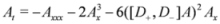
Here, we propose a general approach for the construction of chiral solutions of SUSY extensions. This approach avoids treating SUSY extensions in terms of components of the bosonic field A given in Equation (1). Assuming D+A = 0, we get the chiral property {D+,D-}A = D+D-A = Ax and the Equations (7–9) reduce to


Note that these equations may be evidently treated as classical [14] PDE's, but remains SUSY extensions due to the Grassmannian dependence of the bosonic field A.
The absence of the Grassmannian variables θ+ and θ- derivatives in Equations (10–12) indicates that the odd sectors of chiral solutions should be free from fermionic constraint. This property is in accordance with the integrability of these extensions due to arbitrary bosonization of the fermionic components [15] of the bosonic superfield A.
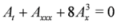
From the classical case, we know that the methods of resolution of all these equations are similar. The same could be said for the SUSY case. Indeed, if we assume the introduction of a potential à such that A = Ãx in Equation (10) and after one integration with respect to x, we get

where the constant of integration is set to zero. The same is done on Equation (12) and leads to
We thus observe that the Equations (11,13,14) are now on an equal footing, i.e., the order of the equation in x is equal to the number of appearance of ∂x in the nonlinear terms. This is standard in Hirota formalism. The choice α = -2 in Equation (13) gives, up to a slight change of variable, the SmKdV Equation (11). This means that the known [7] N super soliton solutions and similarity solutions of SKdV-2 will lead to similar types of solutions for the SmKdV Equation (11).
Now setting

in Equation (13), we obtain

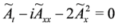
The above equation reduces to the linear dispersive equation [14]

for the special and only values α=1 with β1=i and α=4 with  . For α=-2, Equation (16) writes
. For α=-2, Equation (16) writes 
which does not linearize but can be bilinearized taking β-2=i. It is discussed in the next Section.
A similar change of variable as in Equation (15) but with Ã= βB log HB and  in Equation (14) is assumed and leads to the linear Schrödinger Equation
in Equation (14) is assumed and leads to the linear Schrödinger Equation 
3. SKdV-2 and SmKdV Equations
It is well known [13,14,15,16,17,18,19] that we can generate via the Hirota bilinear formalism N soliton and similarity solutions in the classical case and in SUSY N=1 extensions. Recently, the formalism was adapted to N=2 extensions [4,7,8] by splitting the equation into two N=1 equations, one fermionic and one bosonic. Our approach consists of treating the equation as a N=2 extension without splitting it, but imposing chirality conditions.
Equation (11) can be bilinearized using the Hirota derivative defined as

Indeed, we take à as in Equation (15) with β-2=i and  , where
  are bosonic chiral superfields for i=1,2. Equation (11) leads to the set of bilinear equations
, where are bosonic chiral superfields for i=1,2. Equation (11) leads to the set of bilinear equations 

This set is analogous to the corresponding bilinear equations in the classical mKdV equation [14] but we deal with superfields τ1 and τ2.
In order to get chiral solutions, we have to solve the set of bilinear equations with the additional chiral property D+τi = 0 for i=1,2. It will lead to new solutions of the SmKdV equation which are related to our recent contribution [7].
3.1. N Super Soliton Solutions
The one soliton solution is easily retrieved. Indeed, we cast
where α1 is an even parameter. Ψ1 is a N=2 chiral bosonic superfield defined as

and never appears on this form in other approaches of N = 2 SUSY. The parameters κ1 and ξ1 are, respectively, even and odd. The τ-functions Equation (23) together with Equation (24) solve the set of bilinear Equations (21,22) and give rise to a one super soliton solution. Since D+Ψ1=0, the resulting traveling wave solution is chiral.
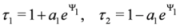
Since we exhibit the three super soliton solution of the SmKdV equation in Figure 1 and Figure 2, we give the general expressions of τ1 and τ2:


Where  and the Ψi's are defined as in Equation (24). The functions τ1 and τ2 solves the bilinear Equations (21) and (22) and are such that D+τi = 0 for i=1,2. The generalization to a N super soliton solution is direct using the τ-functions expressed above. The forms of the τ-functions given above are new representations of super soliton solutions and have never been introduced before.
and the Ψi's are defined as in Equation (24). The functions τ1 and τ2 solves the bilinear Equations (21) and (22) and are such that D+τi = 0 for i=1,2. The generalization to a N super soliton solution is direct using the τ-functions expressed above. The forms of the τ-functions given above are new representations of super soliton solutions and have never been introduced before.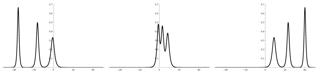
Figure 1.
The function Im(v) of the three soliton solution of the SmKdV equation where  and t = -20,0,20
and t = -20,0,20
Figure 1.
The function Im(v) of the three soliton solution of the SmKdV equation where and t = -20,0,20
and t = -20,0,20

Figure 2.
The density plots of the functions f1, f2 and f3, respectively from left to right, of the three soliton solution of the SmKdV equation where .
.
Figure 2.
The density plots of the functions f1, f2 and f3, respectively from left to right, of the three soliton solution of the SmKdV equation where .
.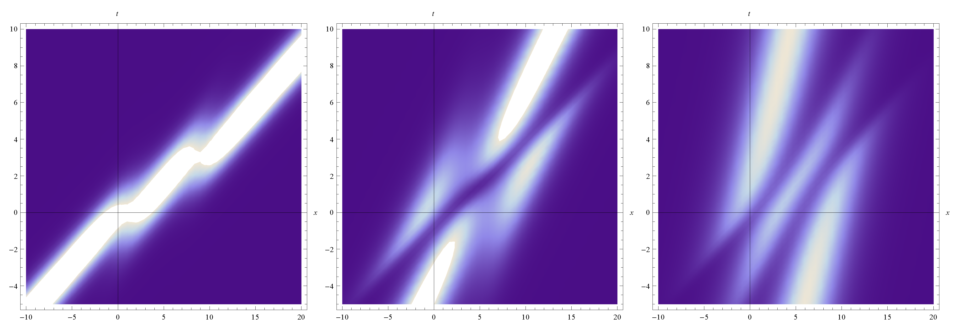
In Figure 1, we may enjoy the three soliton solution Im(v) of the SmKdV equation given by

as a function of x, for the special values , αi=i in Equations (25) and (26) and t=-20,0,20. In Figure 2, we explore the behavior of the fermionic component ρ- of the superfield A for the same special values. To achieve this, we write ρ- as
, αi=i in Equations (25) and (26) and t=-20,0,20. In Figure 2, we explore the behavior of the fermionic component ρ- of the superfield A for the same special values. To achieve this, we write ρ- as 
and trace out the bosonic functions f1, f2 and f3.
3.2. Similarity Solutions
In a recent paper [7], we have proven the existence of an infinite set of rational similarity solutions of the SKdV-2 using a SUSY version of the Yablonskii–Vorob'ev polynomials [16,17,18]. We propose in this subsection to retrieve those solutions and find an infinite set of similarity solution for the SmKdV equation. To give us a hint into what change of variables we have to cast, we have used the symmetry reduction method associated to a dilatation invariance [2].
Let us define the following τ-functions [7]

where  and the functions
  are the Yablonskii–Vorob'ev polynomials defined by the recurrence relation
and the functions are the Yablonskii–Vorob'ev polynomials defined by the recurrence relation 
with  and
and  . We would like to insist that
  is a N=2 bosonic superfield (as it is the case for the Ψi in the preceding subsection). Using the fact that the Yablonskii–Vorob'ev polynomials satisfy the following bilinear equations [17]
and . We would like to insist that is a N=2 bosonic superfield (as it is the case for the Ψi in the preceding subsection). Using the fact that the Yablonskii–Vorob'ev polynomials satisfy the following bilinear equations [17] 

we have that the pair of bilinear Equations (21) and (22) are such that [7,16,17,18]


From the choice of the variable , we also have D+τi,n = 0 for all integers n. Taking τ2,n = τ1,n+1, we have an infinite set of similarity solutions of the SmKdV Equation given by
, we also have D+τi,n = 0 for all integers n. Taking τ2,n = τ1,n+1, we have an infinite set of similarity solutions of the SmKdV Equation given by 
for all integers n ≥ 0 and τ1,n defined as in Equation (29). To get similarity solutions An of the SKdV-2, we use the above solution with  . Plots of some similarity solutions are given in our recent contribution [7].
. Plots of some similarity solutions are given in our recent contribution [7].4. SKdV1, SKdV4 and SB Equations and Virtual Solitons
In this section, we exhibit N super soliton solutions, called N super virtual solitons, for the three equations SKdV1, SKdV4 and SB. Virtual solitons are soliton-like solutions which exhibit no phase shifts in nonlinear interactions. In terms of classical N soliton solutions [3,4,5,7,14,16,19], this is equivalent to say that the interaction coefficients Aij between soliton i and soliton j are zero,  . They manifest as traveling wave solutions for negative time t«0 and decrease spontaneously at time t=0 to split into a N soliton profile which exhibit no phase shifts. It is often said that the traveling wave solution was charged with N-1 soliton, called virtual solitons [5].
. They manifest as traveling wave solutions for negative time t«0 and decrease spontaneously at time t=0 to split into a N soliton profile which exhibit no phase shifts. It is often said that the traveling wave solution was charged with N-1 soliton, called virtual solitons [5].Using the change of variable Equation (15) for the unknown bosonic field Ã, we have seen that the bosonic field Hα must be a chiral superfield and solve the linear dispersive Equation (17) when α=1 and α=4. For the Burgers equation, the bosonic field HB had to be chiral and solves Equation (19).
It is easy to show that they admit the following solution

where the bosonic superfields Ψi are given as
The frequencies ω(κi) are such that ω(κi)= - κi3 for SKdVα and ω(κi)=- κi2 for SB. It looks like a typical KdV type soliton solution where all the interaction coefficients Aij are set to zero.
We see that the virtual soliton solutions of the SKdV1 and SKdV4 equations are completely similar due to the form of à which differs only by the constant value of βα. The expression of the original bosonic field is obtained from

where β=βα for the SKdVα equation and β=βB for the SB equation. Thus, we can give the explicit forms of the superfield components u and ρ-. Indeed, we have

where ηi=κix+ ω(κi)t and the bosonic functions fi(x,t) are defined as

In Figure 3, we may enjoy the three virtual soliton solution Im(u) of the SKdV1 Equation for and αi = 1 in Equation (36) and t= 0,10,20. In Figure 4, we observe the behavior of the function v where v = - iux, and αi=1 in Equation (36) and t=20,0,20. For the same special values, Figure 5 gives the density plots of the bosonic functions f1, f2 and f3 as given in Equation (40).
and αi = 1 in Equation (36) and t= 0,10,20. In Figure 4, we observe the behavior of the function v where v = - iux, and αi=1 in Equation (36) and t=20,0,20. For the same special values, Figure 5 gives the density plots of the bosonic functions f1, f2 and f3 as given in Equation (40).
Figure 3.
The function Im(u) of the three virtual soliton solution of the SKdV1 equation where and t=0,10,20.
and t=0,10,20.
Figure 3.
The function Im(u) of the three virtual soliton solution of the SKdV1 equation where and t=0,10,20.
and t=0,10,20.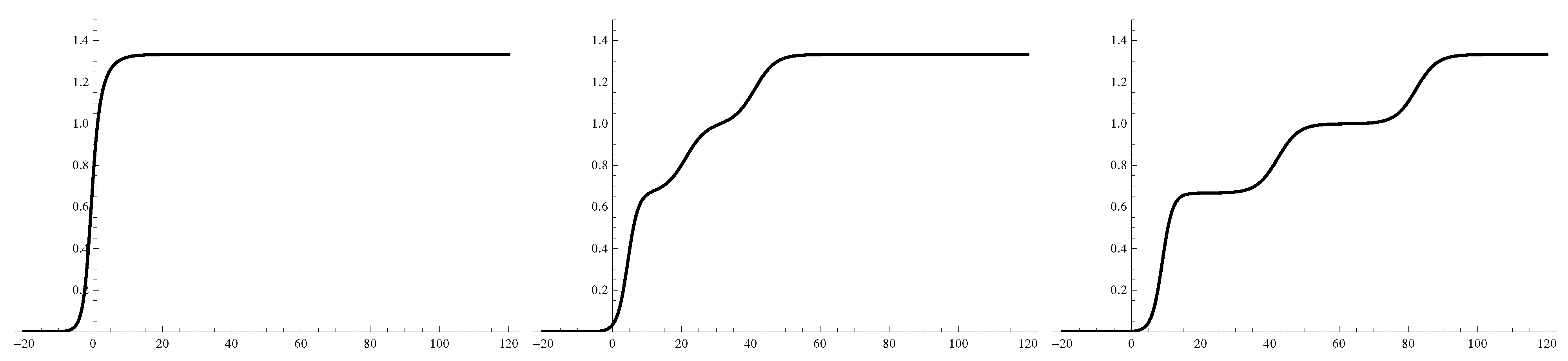

Figure 4.
The function v of the three virtual soliton solution of the SKdV1 equation where and t=20,0,20.
and t=20,0,20.
Figure 4.
The function v of the three virtual soliton solution of the SKdV1 equation where and t=20,0,20.
and t=20,0,20.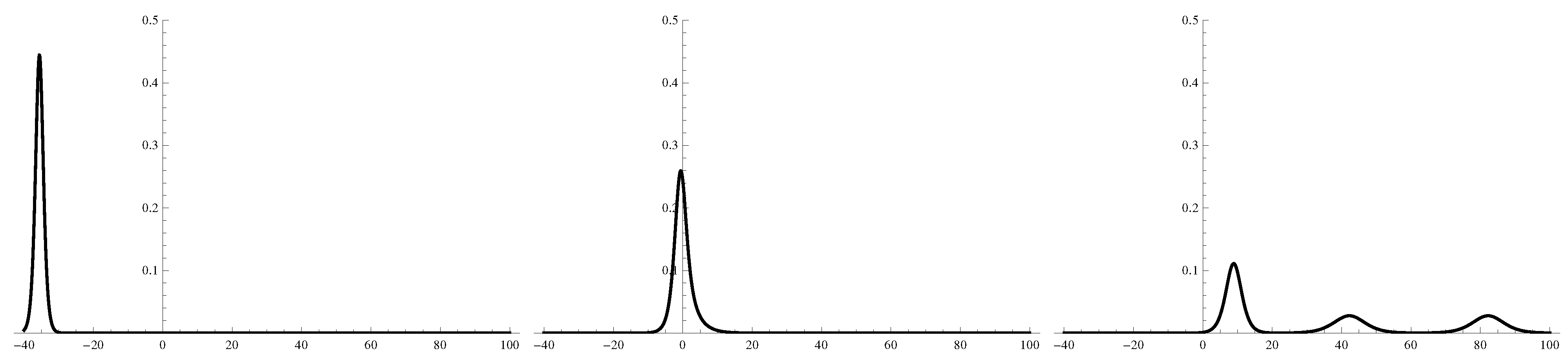
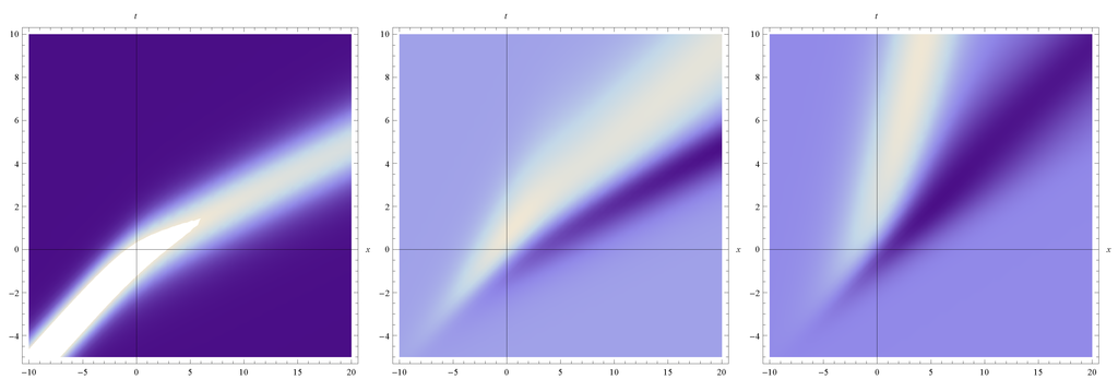
Figure 5.
The density plots of the functions f1, f2 and f3, respectively from left to right, of the three virtual soliton solution of the SKdV1 equation where .
.
Figure 5.
The density plots of the functions f1, f2 and f3, respectively from left to right, of the three virtual soliton solution of the SKdV1 equation where .
.
5. SUSY N=4 KdV Equation and Virtual Solitons
The SUSY N=4 KdV equation, as proposed by Popowicz in [6], reads

where Г is a bosonic superfield and the complex supercovariant derivatives are defined as

where  for i=1,2,3,4. Using the relations {Di,Dj}=2δij∂x, where δij is the Kronecker delta, we have that the supercovariant derivatives Equation (42) satisfy the anticommutation rules
for i=1,2,3,4. Using the relations {Di,Dj}=2δij∂x, where δij is the Kronecker delta, we have that the supercovariant derivatives Equation (42) satisfy the anticommutation rules 
where μ,v ∈ {+,-}. Equation (41) can easily be viewed as a generalization of a N=2 equation. Indeed, setting θ3=θ4=0 and  in Equation (41), we retrieve the SmKdV Equation (8).
in Equation (41), we retrieve the SmKdV Equation (8).To construct virtual solitons of N=2 SUSY extensions, we have considered chiral superfields. Here, we propose a generalization of this concept. Indeed, we impose the following constraints on the superfield Г

A bosonic superfield Ξ satisfying the chiral conditions Equation (44) has the following general form
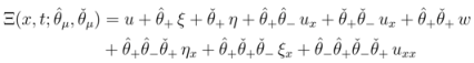
where u=u(x,t) and w=w(x,t) are complex valued bosonic functions and ξ=ξ(x,t) and η=η(x,t) are complex valued fermionic functions. The Grassmann variables in Equation (45) are defined as  and
and  . Now, using the chirality conditions Equation (44), we have
  and Equation (41) reduces to the classical nonlinear PDE
and . Now, using the chirality conditions Equation (44), we have and Equation (41) reduces to the classical nonlinear PDE 
Equation (46) is, up to a slight change of variable, similar to Equation (13) for the integrable cases α=1,4. Indeed, we retrieve Equation (13) for α=1,4by casting  in Equation (46).
in Equation (46).The above equation can be linearized into the linear dispersive Equation (17) by the change of variable

Thus to obtain solutions of Equation (41), the superfield  must satisfy the constraints
must satisfy the constraints 
A solution to this system is

where φ is a N=4 chiral bosonic superfield of the form

with  and λ1 is an even constant. This result can thus be generalized to give a N super virtual soliton solution of the SUSY N=4 KdV Equation (41) by taking
and λ1 is an even constant. This result can thus be generalized to give a N super virtual soliton solution of the SUSY N=4 KdV Equation (41) by taking 
where the superfields φi are defined as in Equation (50) for i=1,…,N.
It is interesting to note that by setting  in Equation (50), one recovers the superfields Equation (24).
in Equation (50), one recovers the superfields Equation (24).6. Concluding Remarks and Future Outlook
In this paper, we have studied special solutions of supersymmetric extensions of the Burgers, KdV and mKdV equations in a unified way and using a chirality of the superfield A.
We have recovered interacting super soliton solutions (often called KdV type solitons) and an infinite set of rational similarity solutions. To produce such rational solutions, we have used an SUSY extension of the Yablonskii–Vorob'ev polynomials. We have introduce a new representation of the τ-functions to solve the bilinear equations. These τ-functions are N=2 extensions of classical τ-functions of the mKdV equation. Till now, in the literature, only N=1 extensions of the τ-functions were given.
We have shown the existence of non-interacting super soliton solutions, called virtual solitons, for the Burgers and SKdVα (α=1,4). These special solutions are a direct generalization of the solutions obtained in a recent contribution [5] where N super virtual solitons have been found by setting to zero the fermionic contributions ξ1 and ξ2 in the bosonic superfield A given as in Equation (1). We retrieve those solutions by setting ςi= 0 in the exponent terms Equation (37). Thus the chirality property, exposed in this paper, has produced a nontrivial fermionic sector for a N super virtual soliton. Furthermore, to obtain such solutions we have related the SUSY equations to linear PDE's showing the true origin of those special solutions.
A N=4 extension of the KdV equation has been shown to produce a N super virtual soliton solution. The study of N=4 extensions is quite new to us and we hope in the future to produce a N super soliton solution with interaction terms.
Acknowledgments
L. Delisle acknowledges the support of a FQRNT doctoral research scholarship. V. Hussin acknowledges the support of research grants from NSERC of Canada.
References
- Labelle, P.; Mathieu, P. A new supersymmetric Korteweg–de Vries equation. J. Math. Phys. 1991, 32, 923–927. [Google Scholar] [CrossRef]
- Ayari, M.A.; Hussin, V.; Winternitz, P. Group invariant solutions for the N=2 super Korteweg–de Vries equation. J. Math. Phys. 1999, 40, 1951–1965. [Google Scholar]
- Ibort, A.; Martinez Alonso, L.; Medina Reus, E. Explicit solutions of supersymmetric KP hierarchies: Supersolitons and solitinos. J. Math. Phys. 1996, 37, 6157–6172. [Google Scholar] [CrossRef]
- Ghosh, S.; Sarma, D. Soliton solutions for the N =2 supersymmetric KdV equation. Phys. Lett. B 2001, 522, 189–193. [Google Scholar] [CrossRef]
- Hussin, V.; Kiselev, A.V. Virtual Hirota' s multi-soliton solutions of N =2 supersymmetric Korteweg–de Vries equations. Theor. Math. Phys. 2009, 159, 832–840. [Google Scholar]
- Popowicz, Z. Odd bihalmitonian structure of new supersymmetric N =2,4 KdV and odd SUSY Virasoro-like algebra. Phys. Lett. B 1999, 459, 150–158. [Google Scholar] [CrossRef]
- Delisle, L.; Hussin, V. New solutions of the N =2 supersymmetric KdV equation via Hirota methods. J. Phys. Conf. Ser. 2012, 343, 012030:1–012030:7. [Google Scholar]
- Zhang, M.-X.; Liu, Q.P.; Shen, Y.-L.; Wu, K. Bilinear approach to N =2 supersymmetric KdV equations. Sci. China Ser. A Math. 2008, 52, 1973–1981. [Google Scholar]
- Gieres, F. Geometry of Supersymmetric Gauge Theories; Lecture Notes in Physics 302; Springer: Berlin/Heidelberg, Germany, 1988. [Google Scholar]
- Grammaticos, B.; Ramani, A.; Lafortune, S. Discrete and continuous linearizable equations. Phys. A 1999, 268, 129–141. [Google Scholar]
- Ramani, A.; Grammaticos, B.; Tremblay, S. Integrable systems without the Painlevé property. J. Phys. A Math. Gen. 2000, 33, 3045–3052. [Google Scholar]
- Carstea, A.S.; Ramani, A.; Grammaticos, B. Linearisable supersymmetric equations. Chaos Soliton. Fract. 2002, 14, 155–158. [Google Scholar] [CrossRef]
- Mc Arthur, I.N.; Yung, C.M. Hirota bilinear form for the super-KdV hierarchy. Mod. Phys. Lett. A 1993, 8, 1739–1745. [Google Scholar] [CrossRef]
- Drazin, P.G.; Johnson, R.S. Solitons: An Introduction; Cambridge University Press: Cambridge, UK, 1989. [Google Scholar]
- Gia, X.N.; Lou, S.Y. Bosonization of supersymmetric KdV equation. Phys. Lett. B 2012, 707, 209–215. [Google Scholar] [CrossRef]
- Ablowitz, M.J.; Satsuma, J. Solitons and rational solutions of nonlinear evolution equations. J. Math. Phys. 1978, 19, 2180–2186. [Google Scholar] [CrossRef]
- Clarkson, P.A. Remarks on the Yablonskii-Vorob'ev polynomials. Phys. Lett. A 2003, 319, 137–144. [Google Scholar] [CrossRef]
- Fukutani, S.; Okamoto, K.; Umemura, H. Special polynomials and the Hirota bilinear relations of the second and the fourth Painlevé equations. Nagoya Math. J 2000, 159, 179–200. [Google Scholar]
- Ghosh, S.; Sarma, D. Bilinearization of N =1 supersymmetric modified KdV equations. Nonlinearity 2003, 16, 411–418. [Google Scholar] [CrossRef]
© 2012 by the authors; licensee MDPI, Basel, Switzerland. This article is an open-access article distributed under the terms and conditions of the Creative Commons Attribution license (http://creativecommons.org/licenses/by/3.0/).