Abstract
A wide range of reaction–diffusion systems with constant diffusivities that are invariant under Q-conditional operators is found. Using the symmetries obtained, the reductions of the corresponding systems to the systems of ODEs are conducted in order to find exact solutions. In particular, the solutions of some reaction–diffusion systems of the Lotka–Volterra type in an explicit form and satisfying Dirichlet boundary conditions are obtained. An biological interpretation is presented in order to show that two different types of interaction between biological species can be described.
1. Introduction
In 1952, Alan Turing published his prominent paper [1]. In this paper he proposed the Turing hypothesis of pattern formation. He used reaction–diffusion equations of the form
which are central to the field of pattern formation.
In system (1), F and G are arbitrary smooth functions, and are unknown functions of the variables t and x, while the subscripts t and x denote differentiation with respect to this variable. Nonlinear system (1) generalizes many well-known nonlinear second-order models used to describe various processes in physics [2], biology [3,4,5] and ecology [6].
Here we concentrate ourselves on the most important subclass of RD systems with the form of (1), namely that with constant coefficients of diffusivity
System (2) has been intensely studied using different mathematical methods (see, e.g., [3,4,7] and papers cited therein). All possible Lie symmetries of system (2) have been found, in [8,9,10,11]. In particular, Q-conditional symmetries of (2) were found in [12]. Reference [13] also contains some results related with system (2).
System (1) is a natural generalization of the well-known RD equation
There are many papers devoted to the construction of Q-conditional symmetries for this equation [14,15,16,17,18,19,20,21], starting from the pioneering work in [22]. There is also a non-trivial generalization of these results for the case of the reaction–diffusion–convection equation ([21] and papers cited therein).
In contrast to (3), there are not many results for searching Q-conditional symmetries of system (2). Construction of the Q-conditional symmetries (non-classical symmetries) of such systems is a very difficult task. Only a few papers have been devoted to the search of such symmetries. In [23] the Q-conditional symmetries of the system
have been obtained; in [24] the Q-conditional symmetries of the Lotka–Volterra system
were obtained.
The paper is organized as follows. In Section 2 three theorems are presented which contain the main result for Q-conditional symmetries of system (2). In Section 3, ansätze for all systems and solutions for one of the systems are derived. In Section 4, the solutions for a generalization of the Lotka–Volterra system are obtained and analyzed. Some graphs of the exact solutions are also presented. Finally, we present some conclusions.
2. Main Result
Let us consider the reaction–diffusion system with constant diffusivities: (2). We want to find Q-conditional operators of the form
under which system (2) is invariant.
The most general form of the Q-conditional operators is
In the case , this operator can be reduced to that with [25]. So we investigate operator (5).
We write down system (2) in the following form:
where
The determining equations for finding coefficients of operator (5) and functions from system (6) have the form
System (7) is an over-determined system of partial differential equations and there are no any general method for solving of such systems [26,27]. Thus, we were not able to find the general solution of system (7), hence we have solved it with conditions
Solving Equations – of system (7), we obtain
where are arbitrary constants, are arbitrary smooth functions. Substituting (9) into from (7) and splitting the obtained equations with respect to the powers of u and v, we arrive at the system
Obviously, that solutions of first pair of equations of (10) will be , or .
Let us consider the case (the case will be considered later). In this case we obtain . Substituting (9) into Equations and of system (7) and splitting with respect to the powers of u and v, we arrive at
Since , we conclude that . Consider the case , (the case , is symmetrical). From Equation , we obtain . Substituting (9) with the specified coefficients, namely
into Equations of system (7), we arrive at
Substituting , obtained from (12), into the third equation of system (11), we obtain , that is , but that contradicts the above restrictions.
Thus, in the case we do not obtain any Q-conditional operator of the form (5).
Consider the case . In this case, from Equations and of system (7), we obtain
where are the arbitrary constants. Thus, expressions (9) take the form
Substituting (13) into Equations and of system (7), we arrive at
Solving the system of algebraic Equations (14), we obtain three solutions and therefore we obtain three cases. Let us consider all these cases.
Theorem 1. In the cases or with conditions (8), the system of determining equations for finding of the Q-conditional operators of the form (5) for system (6) coincide with the system of determining equations for finding Lie operators.
Proof. Substituting (13), with , into system (7) we find that Equations are transformed into identities, and Equations and take the form
In [11] the determining equations for finding of Lie symmetries with condition are written down in explicit form. Substituting conditions (8) into these equations, we see that the result is completely identical to Equations (15).
Substituting (13), with into system (7), we see that Equations also transform into identities, and equations and take the form
Comparing equations (16) with equations for finding of Lie symmetries of system (6) with conditions (8) from [9], we see that they are completely identical. ☐
Thus, in the following we assume that
Let us consider the case , which is on the one hand the most interesting and on the other the most difficult. In this case, (13) takes the form
Equations satisfy expressions (17) and Equations take the form
Thus, we can formulate the following theorem.
Theorem 2. The nonlinear reaction–diffusion system (6) is Q-conditionally invariant under operator (5) with coefficients (17) if and only if the nonlinearities are the solutions of linear system (18).
To find the general solution of system (18), one need to analyze two cases and . In the case , system (18) takes the form
Since , renaming , and , and taking into account that with any coefficients , we can remove the parameter using linear substitutions of , system (19) reduces to the form
One notes a particular solution of system (20), of the form
Now to construct the general solution of (20), we need to solve the corresponding homogeneous system, that is
As a result, the following statement was proved.
Theorem 3. Reaction–diffusion system (6) is Q-conditionally invariant under operator (5) with conditions (8), and , if and only if the system and corresponding operator have one of the seven following forms (moreover ):
Proof. To prove this theorem, it is necessary and sufficient to construct the general solution of system (22) for all possible ratios between parameters To do this we need to investigate the following seven cases:
1. ;
2. ;
3. ;
4. ;
5. .
6. ;
7. .
These cases take into account all possibilities that arise when we solve system (22). Let us consider these cases.
Case 1. Solving the second equation of (22), we get and . So the first equation of (22) reduces to an ODE for finding of the function :
Solving it, we get that Taking into account the expressions for obtained above, from Formulas (21) and restrictions (obtained above), finally we arrive at the reaction–diffusion system and the Q-conditional operator listed in (23) of Theorem 3.
Cases 2–7. Considering similarly these cases and using simple renamings, we arrive at systems and operators (24)–(29) of Theorem 3. ☐
In the case we should also assume that , otherwise we obtain the case up to renaming. We seek a solution of system (18) of the form
Substituting (30) into (18), we obtain the system of algebraic equations
Solving system (31), we arrive at two possibilities depending on :
I)
II)
In Case I) , we obtain the solution of system (18)
In Case II) we obtain the solution of system (18)
Furthermore, we must solve the homogeneous system
Let us consider Case I). Using the condition for system (34), we get
Multiplying the second equation of (35) by , adding to the first and renaming , we arrive at
Using the substitution
we obtain the equation
Solving Equation (38), we arrive at three subcases:
1)
2)
3)
Substituting (37) together with the function S from subcase 1) into the second equation of (35), we obtain
Solving (39), using (37), (32) and renaming we obtain the system
Q-conditionally invariant under the operator
Similarly, for subcase 2), we arrive at the system
and the operator
In the subcase 3), we obtain the system
and the operator
Examination of Case II) is highly nontrivial and will be reported in another paper.
3. Ansätze and Exact Solutions of the Reaction–Diffusion System
Using standard procedures, we obtain ansätze for all operators of Theorem 3. Substituting these anzätze in the corresponding reaction–diffusion systems, we obtain the reduction systems of equations. All anzätze and reduction systems are presented in Table 1.

Table 1.
Ansätze and reduction systems of Theorem 3.
| No. | Ansätze | Systems of ODEs |
|---|---|---|
| (23) | ||
| (24) | ||
| (25) | ||
| (26) | ||
| (27) | ||
| (28) | ||
| (29) | ||
It is impossible to find the general solution of the systems from Table 1 for arbitrary functions g and h. However, if we correctly specify these functions we can find the solutions of these systems.
System (27) is the most interesting one from the point of view of applicability. Let us consider system (27) with . In this case, the reduction system has the form
The solution of Equation (41) has the form
The solutions of Equation (43) depend on the parameter A. Solving Equation (43) we get three different solutions (up to transformations )
Substituting φ and (42) into corresponding ansatz from Table 1, and renaming , we arrive at the exact solutions
of the reaction–diffusion system
where k is the solution of the equation
4. Solutions and Their Properties of Some Generalization of the Lotka–Volterra System
Let us consider in detail the case . Renaming , we obtain the exact solution
where and k is the solution of , of the reaction–diffusion system
where
System (47) is the generalized Lotka–Volterra system. With system (47) becomes the classical Lotka–Volterra system
Note that exact solutions of the form (46) for the classical Lotka–Volterra system (48) have been found in [24].
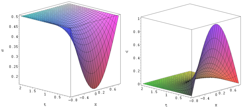
Figure 1.
Exact solution to (51).
Figure 1.
Exact solution to (51).

System (48) can be obtained from system (47) with Also, the coefficients of (46) and (48) must satisfy the equation
It is well known [3] that three main kinds of interactions between two biological species are simulated by system (48):
(i) predator u–prey v interaction,
(ii) competition of the species,
(iii) mutualism or symbiosis.
It turns out that solution (46) can describe the predator-prey interaction on the space interval , (here ) provided that
One can easily check that solution (46) is non-negative, bounded in the domain and satisfies the given Dirichlet boundary conditions, i.e.,
Choosing the coefficients , gives that Thus, from solution (46) we obtain the solution
of the system
which can describe predator u–prey v interaction, as its coefficients satisfy the conditions for this type of the interaction [3]. System (52) is some generalization of the Lotka–Volterra system (48) with additional nonlinearity in the first equation.
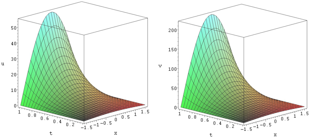
Figure 2.
Exact solution of (55).
Figure 2.
Exact solution of (55).

As an example, we present solution (51) in Figure 1. This solution can describe the predator u–prey v interaction between the species u and v when population of predator u becomes and prey eventually dies, i.e., as .
Choosing coefficients , we get Renaming , from solution (46) we obtain the solution
of the system
which can also describe the predator u–prey v interaction, as its coefficients satisfy conditions for this type of interaction [3]. System (52) is some generalization of Lotka–Volterra system (48) with additional nonlinearity in the first equation.
Solution (53) satisfies Dirichlet boundary conditions (50) with and . This solution can describe the predator u–prey v interaction between the species u and v when population of predator u becomes 1 and prey eventually die, i.e., as .
If we consider system (48) with solution (46), then we obtain the solution that can describe competition of the species. Such a solution is presented in [24].
5. Conclusions
In this paper, the nonlinear RD system (2) was examined in order to find the Q-conditional operators under which this system is invariant and to construct exact solutions. Because the system of differential (7) is too complicated, we were unable (and believe it is not possible) to find all the solutions of the determining system (7) and thence to find all possible Q-conditional operators. We have found the Q–conditional operators with restrictions (8) (in the case we have found all possible systems and operators, in the case we have presented some examples) with respect to which the reaction–diffusion system of equations with constant diffusion (2) is invariant. All these operators are given in Theorem 3 of Section 2. In Section 3 the ansätze for all Q-conditional operators of Theorem 3 and the reduction systems are constructed. Section 4 contains the solutions of some generalization of the Lotka–Volterra system. These solutions are analyzed in order to present of biological interpretation. Some graphs of obtained solutions are also presented. It is shown that the obtained solutions satisfy Dirichlet boundary conditions, which are typical for biological interpretation.
Acknowledgments
The author is grateful to the referees for the useful comments.
Conflicts of Interest
The author declares no conflict of interest.
References
- Turing, A.M. The chemical basis of morphogenesis. Philos. Trans. Royal Soc. Lond. B Biol. Sci. 1952, 237, 37–72. [Google Scholar] [CrossRef]
- Ames, W.F. Nonlinear Partial Differential Equations in Engineering; Academic Press: New York, NY, USA; London, UK, 1965; p. xii+511. [Google Scholar]
- Murray, J.D. Mathematical Biology I: An Introduction, 3rd ed.; Interdisciplinary Applied Mathematics; Springer-Verlag: New York, NY, USA, 2002; Volume 17, p. xxiv+551. [Google Scholar]
- Murray, J.D. Mathematical biology II: Spatial Models and Biomedical Applications, 3rd ed.; Interdisciplinary Applied Mathematics; Springer-Verlag: New York, NY, USA, 2003; Volume 18, p. xxvi+811. [Google Scholar]
- Britton, N.F. Essential Mathematical Biology; Springer Undergraduate Mathematics Series; Springer-Verlag London, Ltd.: London, UK, 2003; p. xvi+335. [Google Scholar]
- Okubo, A.; Levin, S.A. Diffusion and Ecological Problems: Modern Perspectives, 2nd ed.; Interdisciplinary Applied Mathematics; Springer-Verlag: New York, NY, USA, 2001; Volume 14, p. xx+467. [Google Scholar]
- Henry, D. Geometric Theory of Semilinear Parabolic Equations; Lecture Notes in Mathematics; Springer-Verlag: Berlin, Germany; New York, NY, USA, 1981; Volume 840, p. iv+348. [Google Scholar]
- Cherniha, R. Lie symmetries of nonlinear two-dimensional reaction–diffusion systems. Rep. Math. Phys. 2000, 46, 63–76. [Google Scholar] [CrossRef]
- Cherniha, R.; King, J.R. Lie symmetries of nonlinear multidimensional reaction–diffusion systems. I. J. Phys. A 2000, 33, 267–282. [Google Scholar] [CrossRef]
- Cherniha, R.; King, J.R. Addendum: “Lie symmetries of nonlinear multidimensional reaction–diffusion systems. I”. J. Phys. A 2000, 33, 7839–7841. [Google Scholar] [CrossRef]
- Cherniha, R.; King, J.R. Lie symmetries of nonlinear multidimensional reaction–diffusion systems. II. J. Phys. A 2003, 36, 405–425. [Google Scholar] [CrossRef]
- Barannik, T.A. Conditional symmetry and exact solutions of a multidimensional diffusion equation. Ukr. Math. J. 2002, 54, 1416–1420. [Google Scholar]
- Barannyk, T. Symmetry and exact solutions for systems of nonlinear reaction–diffusion equations. Available online: http://eqworld.ipmnet.ru/en/solutions/interesting/barannyk.pdf (accessed on 13 October 2015).
- Serov, N.I. Conditional invariance and exact solutions of a nonlinear heat equation. Ukr. Math. J. 1990, 42, 1370–1376. [Google Scholar]
- Fushchych, W.; Shtelen, W.; Serov, M. Symmetry Analysis and Exact Solutions of Equations of Nonlinear Mathematical Physics; Kluwer: Dordrecht, The Netherland, 1993. [Google Scholar]
- Nucci, M.C. Symmetries of linear, C-integrable, S-integrable, and nonintegrable equations. In Nonlinear Evolution Equations and Dynamical Systems (Baia Verde, 1991); World Sci. Publ.: River Edge, NJ, USA, 1992; pp. 374–381. [Google Scholar]
- Clarkson, P.A.; Mansfield, E.L. Symmetry reductions and exact solutions of a class of nonlinear heat equations. Physica D 1994, 70, 250–288. [Google Scholar] [CrossRef]
- Arrigo, D.J.; Hill, J.M.; Broadbridge, P. Nonclassical symmetry reductions of the linear diffusion equation with a nonlinear source. IMA J. Appl. Math. 1994, 52, 1–24. [Google Scholar] [CrossRef]
- Arrigo, D.J.; Hill, J.M. Nonclassical symmetries for nonlinear diffusion and absorption. Stud. Appl. Math. 1995, 94, 21–39. [Google Scholar] [CrossRef]
- Pucci, E.; Saccomandi, G. Evolution equations, invariant surface conditions and functional separation of variables. Physica D 2000, 139, 28–47. [Google Scholar] [CrossRef]
- Bluman, G.W.; Cheviakov, A.F.; Anco, S.C. Applications of Symmetry Methods to Partial Differential Equations; Applied Mathematical Sciences; Springer: New York, NY, USA, 2010; Volume 168. [Google Scholar]
- Bluman, G.W.; Cole, J.D. The general similarity solution of the heat equation. J. Math. Mech. 1968/69, 18, 1025–1042. [Google Scholar]
- Cherniha, R.; Pliukhin, O. New conditional symmetries and exact solutions of reaction–diffusion systems with power diffusivities. J. Phys. A 2008, 41, 185208:1–185208:14. [Google Scholar] [CrossRef]
- Cherniha, R.; Davydovych, V. Conditional symmetries and exact solutions of the diffusive Lotka–Volterra system. Math. Comput. Model. 2011, 54, 1238–1251. [Google Scholar] [CrossRef]
- Cherniha, R. Conditional symmetries for systems of PDEs: New definitions and their application for reaction–diffusion systems. J. Phys. A 2010, 43, 405207:1–405207:13. [Google Scholar] [CrossRef]
- Sidorov, A.F.; Shapeev, V.P.; Yanenko, N.N. Metod Differentsialnykh Svyazei i Ego Prilozheniya v Gazovoi Dinamike; “Nauka” Sibirsk. Otdel.: Novosibirsk, Russia, 1984; p. 272. (In Russian) [Google Scholar]
- Carini, M.; Fusco, D.; Manganaro, N. Wave-like solutions for a class of parabolic models. Nonlinear Dynam. 2003, 32, 211–222. [Google Scholar] [CrossRef]
© 2015 by the authors; licensee MDPI, Basel, Switzerland. This article is an open access article distributed under the terms and conditions of the Creative Commons Attribution license (http://creativecommons.org/licenses/by/4.0/).