Centrally Extended Conformal Galilei Algebras and Invariant Nonlinear PDEs

Abstract

We construct, for any given $\ell =\frac{1}{2}+{\mathbb{N}}_0,$ second-order nonlinear partial differential equations (PDEs) which are invariant under the transformations generated by the centrally extended conformal Galilei algebras. This is done for a particular realization of the algebras obtained by coset construction and we employ the standard Lie point symmetry technique for the construction of PDEs. It is observed that the invariant PDEs have significant difference for $\ell >\frac{3}{2}.$

1. Introduction

The purpose of the present work is to construct partial differential equations (PDEs) which are invariant under the transformations generated by the conformal Galilei algebra (CGA). We consider a particular realization, which is given in [1], of CGAs with the central extension for the parameters $(d,\ell )=(1,\frac{1}{2}+{\mathbb{N}}_0),$ where ${\mathbb{N}}_0$ denotes the set of non-negative integers. We also restrict ourselves to the second-order PDEs for computational simplicity. Our main focus is on nonlinear PDEs since linear ones have already been discussed in the literatures [1,2,3,4]. CGA is a Lie algebra which generates conformal transformations in $d+1$ dimensional nonrelativistic spacetime [5,6,7,8]. Even in the fixed dimension of spacetime one has infinite number of inequivalent conformal algebras. For a fixed value of d each inequivalent CGA is labelled by a parameter ℓ taking the spin value, i.e., $\ell =\frac{1}{2},1,\frac{3}{2},2,\dots .$ Each CGA has an Abelian ideal (namely, CGA is a non-semisimple Lie algebra) so that it would be deformed. Indeed, it has a central extension depending the value of the parameters. More precisely, there exist two different types of central extensions. One of them exists for any values of d and half-integer $\ell ,$ another type of extension exists for $d=2$ and integer $\ell .$ Simple explanation of this fact is found in [9].

It has been observed that CGAs for $\ell =\frac{1}{2}$ and $\ell =1$ play important roles in various kind of problems in physics and mathematics. The simplest $\ell =\frac{1}{2}$ member of CGAs is called the Schrödinger algebra which was originally discussed by Sophus Lie and Jacobi in 19th century [10,11] and reintroduced later by many physicists [12,13,14,15,16,17]. Recent renewed interest in CGAs is mainly due to the AdS/CFT correspondence. The Schrödinger algebra and $\ell =1$ member of CGA were used to formulate nonrelativistic analogues of AdS/CFT correspondence [9,18,19]. One may find a nice review of various applications of the Schrödinger algebras in [20] and see [21] for more references on the Schrödinger algebras and $\ell =1$ CGAs. Physical applications of $\ell =2$ CGA is found in [22].

Now one may ask a question whether the CGAs with $\ell >1$ are relevant structures to physical or mathematical problems. To answer this question one should find classical or quantum dynamical systems relating to CGAs and develop representation theory of CGAs (see [21,23,24] for classification of irreducible modules over $d=1,2$ CGAs ). This is the motivation of the present work. We choose a particular differential realization of CGAs then look for PDEs invariant under the transformation generated by the realization. Investigation along this line for the Schrödinger algebras is found in [2,3,25,26,27] and for $\ell =1$ CGAs in [28] and for related algebraic structure in [29,30]. For higher values of ℓ use of the representation theory such as Verma modules, singular vectors allows us to derive linear PDEs invariant under CGAs [1,4]. More physical applications of CGAs with higher value ℓ are found in the literatures [31,32,33,34,35,36,37,38,39,40,41,42,43,44,45].

The paper is organized as follows. In the next section the definition of CGA for $(d,\ell )=(1,\frac{1}{2}+{\mathbb{N}}_0)$ and its differential realization are given. Then symmetry of PDEs under a subset of the generators is considered. It is shown that there is a significant distinction of the form of invariant PDEs for $\ell >\frac{3}{2}.$ Invariant PDEs for $\ell =\frac{3}{2}$ CGA are obtained in Section 3 For $\ell \ge \frac{5}{2}$ we first derive PDEs invariant under a subalgebra of the CGA in Section 4, then derive invariant PDEs under full CGA in Section 5. Section 6 is devoted to concluding remarks.

2. CGAs and Preliminary Consideration

The CGA for $d=1$ and any half-integer ℓ consists of $sl(2,\mathbb{R})\simeq so(2,1)=⟨H,D,C⟩$ and $\ell +1/2$ copies of the Heisenberg algebra ${⟨P^{\left(n\right)},M⟩}_{n=1,2,\dots ,2\ell +1}.$ Their nonvanishing commutators are given by

$$\begin{array}{c}[D,H]=-2H,[D,C]=2C,[H,C]=D,\hfill \\ [H,P^{\left(n\right)}]=(n-1)P^{(n-1)},[D,P^{\left(n\right)}]=2(n-1-\ell )P^{\left(n\right)},\hfill \\ [C,P^{\left(n\right)}]=(n-1-2\ell )P^{(n+1)},[P^{\left(m\right)},P^{\left(n\right)}]=-{\delta }_{m+n,2\ell +2}{I}_{m-1}M\hfill \end{array}$$

(1)

where the structure constant $I_m$ is taken to be $I_m={(-1)}^{m+\ell +\frac{1}{2}}(2\ell -m)!m!$ and M is the centre of the algebra. We denote this algebra by ${\mathfrak{g}}_{\ell }$. The subset ${⟨P^{\left(n\right)},M,H⟩}_{n=1,2,\dots ,2\ell +1}$ forms a subalgebra of ${\mathfrak{g}}_{\ell }$ and we denote it by ${\mathfrak{h}}_{\ell }.$

We employ the following realization of ${\mathfrak{g}}_{\ell }$ on the space of functions of the variables $t=x_0,x_1,\dots ,x_{\ell +\frac{1}{2}}$ and U [1]:

$$\begin{array}{c}M=U{\partial }_U,D=2t{\partial }_t+\sum _{k=1}^{\ell +\frac{1}{2}}2(\ell +1-k)x_k{\partial }_{x_k},H={\partial }_t,\hfill \end{array}$$

$$\begin{array}{c}C=t^2{\partial }_t+\sum _{k=1}^{\ell +\frac{1}{2}}2(\ell +1-k)t{x}_k{\partial }_{x_k}+\sum _{k=1}^{\ell -\frac{1}{2}}(2\ell +1-k)x_k{\partial }_{x_{k+1}}-\frac{1}{2}{\left(\left(\ell +\frac{1}{2}\right)!\right)}^2{x}_{\ell +\frac{1}{2}}^{2}U{\partial }_U,\hfill \end{array}$$

$$\begin{array}{c}{P}^{\left(n\right)}=\sum _{k=1}^n\left(\genfrac{}{}{0pt}{}{n-1}{k-1}\right)t^{n-k}{\partial }_{x_k},1\le n\le \ell +\frac{1}{2},\hfill \end{array}$$

(2)

$$\begin{array}{c}{P}^{\left(n\right)}=\sum _{k=1}^{\ell +\frac{1}{2}}\left(\genfrac{}{}{0pt}{}{n-1}{k-1}\right)t^{n-k}{\partial }_{x_k}-\sum _{k=\ell +\frac{3}{2}}^n\left(\genfrac{}{}{0pt}{}{n-1}{k-1}\right)I_{k-1}{t}^{n-k}{x}_{2\ell +2-k}U{\partial }_U,\ell +\frac{3}{2}\le n\le 2\ell +1\hfill \end{array}$$

where $\left(\genfrac{}{}{0pt}{}{n}{k}\right)$ is the binomial coefficient and $I_{k-1}$ is the structure constant appearing in Equation (1). This is in fact a realization of ${\mathfrak{g}}_{\ell }$ on the Borel subgroup of the conformal Galilei group generated by ${\mathfrak{g}}_{\ell }$ (we made some slight changes from [1]). Let us introduce the sets of indices for later convenience:

$${\mathcal{I}}_{\mu }=\left\{\mu ,\mu +1,\dots ,\ell +\frac{1}{2}\right\},\mu =0,1,2,\dots$$

(3)

Now we take $x_{\mu },\mu \in {\mathcal{I}}_0$ as independent variables and U as dependent variable: $U=U\left(x_{\mu }\right).$ Our aim is to find second order PDEs which are invariant under the point transformations generated by Equation (2) for $\ell >1/2$ ($\ell =1/2$ corresponds to Schrödinger algebra). Such a PDE is denoted by

$$F(x_{\mu },U,U_{\mu },U_{\mu \nu })=0,U_{\mu }=\frac{\partial U}{\partial x_{\mu }},U_{\mu \nu }=\frac{{\partial }^{2}U}{\partial x_{\mu }{x}_{\nu }}$$

(4)

We use the shorthand notation throughout this article. The left hand side of Equation (4) means that F is a function of all independent variables $x_{\mu },\mu \in {\mathcal{I}}_0,$ dependent variable U and all first and second order derivatives of $U.$ As found in the standard textbooks (e.g., [46,47,48]) the symmetry condition is expressed in terms of the prolonged generators:

$$\widehat{X}F=0(\mathrm{mod} F=0)$$

(5)

where $\widehat{X}$ is the prolongation of the symmetry generator X up to second order:

$$\widehat{X}=X+\sum _{\mu =0}^{\ell +\frac{1}{2}}{\rho }^{\mu }\frac{\partial }{\partial U_{\mu }}+\sum _{\mu \le \nu }{\sigma }^{\mu \nu }\frac{\partial }{\partial U_{\mu \nu }},X=\sum _{\mu =0}^{\ell +\frac{1}{2}}{\xi }^{\mu }\frac{\partial }{\partial x_{\mu }}+\eta \frac{\partial }{\partial U}$$

(6)

The quantities ${\rho }^{\mu },{\sigma }^{\mu \nu }$ are defined by

$$\begin{array}{ccc}\hfill {\rho }^{\mu }& =& {\eta }_{\mu }+{\eta }_U{U}_{\mu }-\sum _{\nu =0}^{\ell +\frac{1}{2}}{U}_{\nu }({\xi }_{\mu }^{\nu }+{\xi }_U^{\nu }{U}_{\mu }),\hfill \end{array}$$

(7)

$$\begin{array}{ccc}\hfill {\sigma }^{\mu \nu }& =& {\eta }_{\mu \nu }+{\eta }_{\mu U}{U}_{\nu }+{\eta }_{\nu U}{U}_{\mu }+{\eta }_U{U}_{\mu \nu }+{\eta }_{UU}{U}_{\mu }{U}_{\nu }\hfill \\ & -& \sum _{\tau =0}^{\ell +\frac{1}{2}}{\xi }_{\mu \nu }^{\tau }{U}_{\tau }-\sum _{\tau =0}^{\ell +\frac{1}{2}}({\xi }_{\mu }^{\tau }{U}_{\nu \tau }+{\xi }_{\nu }^{\tau }{U}_{\mu \tau })-\sum _{\tau =0}^{\ell +\frac{1}{2}}{\xi }_U^{\tau }(U_{\tau }{U}_{\mu \nu }+U_{\mu }{U}_{\nu \tau }+U_{\nu }{U}_{\mu \tau })\hfill \\ & -& \sum _{\tau =0}^{\ell +\frac{1}{2}}({\xi }_{\mu U}^{\tau }{U}_{\nu }+{\xi }_{\nu U}^{\tau }{U}_{\mu }+{\xi }_{UU}^{\tau }{U}_{\mu }{U}_{\nu })U_{\tau }\hfill \end{array}$$

(8)

In this section we consider the symmetry condition Equation (5) for $M,H$ and $P^{\left(n\right)}$ with $n=1,2,\dots ,2\ell +1.$

Lemma 1. (i) Equation (4) is invariant under $H,P^{\left(1\right)}$ and M if it has the form

$$F\left(x_a,\frac{U_{\mu }}{U},\frac{U_{\mu \nu }}{U}\right)=0,a\in {\mathcal{I}}_2,\mu ,\nu \in {\mathcal{I}}_0$$

(9)

(ii) 

For $\ell >\frac{3}{2},$ a necessary condition for the symmetry of the Equation (9) under $P^{\left(n\right)}$ with $n\in {\mathcal{I}}_2$ is that the function F is independent of $U_{0m},m\in {\mathcal{I}}_3.$

Proof of Lemma 1. (i) It is obvious from that the generators H and $P^{\left(1\right)}$ have no prolongation, while the prolongation of M is given by

$$\widehat{M}=U{\partial }_U+\sum _{\mu =0}^{\ell +\frac{1}{2}}{U}_{\mu }{\partial }_{U_{\mu }}+\sum _{\mu \le \nu }{U}_{\mu \nu }{\partial }_{U_{\mu \nu }}$$

(10)

(ii) The lemma is proved by the formula of the prolongation of $P^{\left(n\right)}.$ For $n\in {\mathcal{I}}_2$ the generator $P^{\left(n\right)}$ is given by

$$P^{\left(n\right)}=\sum _{k=1}^n\left(\genfrac{}{}{0pt}{}{n-1}{k-1}\right)t^{n-k}{\partial }_{x_k}$$

and its prolongation yields

$${\widehat{P}}^{\left(n\right)}=\sum _{a=2}^n\left(\begin{array}{c}n-1\\ n-a\end{array}\right)t^{n-a}\left[{\tilde{P}}^{\left(a\right)}-\sum _{k=a+1}^n(a-1)U_{a-1k}{\partial }_{U_{0k}}\right]$$

(11)

where

$${\tilde{P}}^{\left(n\right)}={\left.{\widehat{P}}^{\left(n\right)}\right|}_{t=0}={\partial }_{x_n}-(n-1)\left\{U_{n-1}{\partial }_{U_0}+\left((n-2)U_{n-2}+2U_{0n-1}\right){\partial }_{U_{00}}+\sum _{k=1}^n{U}_{n-1k}{\partial }_{U_{0k}}\right\}$$

(12)

and the terms containing ${\partial }_{x_1}$ are omitted. We give the explicit expressions for small values of n which will be helpful to see the structure of Equation (11):

$$\begin{array}{ccc}\hfill {\widehat{P}}^{\left(2\right)}& =& {\tilde{P}}^{\left(2\right)},\hfill \\ \hfill {\widehat{P}}^{\left(3\right)}& =& {\tilde{P}}^{\left(3\right)}+2t({\tilde{P}}^{\left(2\right)}-U_{13}{\partial }_{U_{03}}),\hfill \\ \hfill {\widehat{P}}^{\left(4\right)}& =& {\tilde{P}}^{\left(4\right)}+3t({\tilde{P}}^{\left(3\right)}-2U_{24}{\partial }_{U_{04}})+3t^2({\tilde{P}}^{\left(2\right)}-U_{13}{\partial }_{U_{03}}-U_{14}{\partial }_{U_{04}})\hfill \end{array}$$

Since ${\tilde{P}}^{\left(n\right)}$ is independent of $t,$ each symmetry condition ${\widehat{P}}^{\left(n\right)}F=0$ decouples into some independent equations. For example, ${\widehat{P}}^{\left(4\right)}F=0$ decouples into the following equations:

$${\tilde{P}}^{\left(4\right)}F=0,({\tilde{P}}^{\left(3\right)}-2U_{24}{\partial }_{U_{04}})F=0,({\tilde{P}}^{\left(2\right)}-U_{13}{\partial }_{U_{03}}-U_{14}{\partial }_{U_{04}})F=0$$

The condition ${\widehat{P}}^{\left(2\right)}F=0$ is equivalent to the condition ${\tilde{P}}^{\left(2\right)}F=0.$ It follows that the condition ${\widehat{P}}^{\left(3\right)}F=0$ yields two independent conditions ${\tilde{P}}^{\left(3\right)}F=0$ and $U_{13}{\partial }_{U_{03}}F=0.$ The second condition means that F is independent of $U_{03}.$ Repeating this for ${\widehat{P}}^{\left(n\right)}F=0$ for $n=4,5,\dots ,\ell +\frac{1}{2}$ one may prove the lemma.

Now we show the Equation (11). Set ${\xi }^k\left(n\right)=\left(\begin{array}{c}n-1\\ k-1\end{array}\right)t^{n-k}$ then ${\displaystyle P^{\left(n\right)}=\sum _{k=2}^n{\xi }^k\left(n\right){\partial }_{x_k}}$ (recall that we omit ${\partial }_{x_1}$). By the EquationS (6)–(8) we have

$${\widehat{P}}^{\left(n\right)}=P^{\left(n\right)}-\sum _{k=1}^n\left\{{\xi }_0^k\left(n\right)U_k{\partial }_{U_0}+({\xi }_{00}^k\left(n\right)U_k+2{\xi }_0^k\left(n\right)U_{0k}){\partial }_{U_{00}}+\sum _{m=1}^n{\xi }_0^m\left(n\right)U_{mk}{\partial }_{U_{mk}}\right\}$$

(13)

Thus the maximal degree of t in ${\widehat{P}}^{\left(n\right)}$ is $n-2.$ The following relation is easily verified:

$$\frac{{\partial }^a}{\partial t^a}{\xi }^k\left(n\right)=\left\{\begin{array}{ccc}\frac{(n-1)!}{(n-a-1)!}{\xi }^k(n-a),\hfill & & (1\le k\le n-a)\hfill \\ 0,\hfill & & (n-a<k)\hfill \end{array}\right.$$

(14)

Using this one may calculate the higher order derivatives of Equation (13):

$$\frac{{\partial }^a}{\partial t^a}{\widehat{P}}^{\left(n\right)}=\frac{(n-1)!}{(n-a-1)!}\left\{P^{(n-a)}-\sum _{k=n-a+1}^n\sum _{m=1}^{n-a}{\xi }_0^m(n-a)U_{mk}{\partial }_{U_{0k}}\right\}$$

It follows that

$$\begin{array}{ccc}\hfill {\widehat{P}}^{\left(n\right)}& =& \sum _{a=0}^{n-2}\frac{1}{a!}{\left(\frac{{\partial }^a}{\partial t^a}{\widehat{P}}^{\left(n\right)}\right)}_{t=0}{t}^a\hfill \\ & =& \sum _{a=0}^{n-2}\left(\begin{array}{c}n-1\\ a\end{array}\right)t^a\left[{\tilde{P}}^{(n-a)}-\sum _{k=n-a+1}^n(n-a-1)U_{n-a-1k}{\partial }_{U_{0k}}\right]\hfill \end{array}$$

By replacing $n-a$ with a we obtain the Equation (11). The Equation (12) is readily obtained by setting $t=0$ in the Equation (13).   □

Remark 1. By Lemma 1 the symmetry condition for $M,H,P^{\left(n\right)}$ with $n\in {\mathcal{I}}_1$ is summarized as

$${\tilde{P}}^{\left(n\right)}F\left(x_a,\frac{U_{\mu }}{U},\frac{U_{00}}{U},\frac{U_{01}}{U},\frac{U_{02}}{U},\frac{U_{km}}{U},\right)=0,a\in {\mathcal{I}}_2,\mu \in {\mathcal{I}}_0,k,m\in {\mathcal{I}}_1$$

(15)

where ${\tilde{P}}^{\left(n\right)}$ is given by Equation (12).

The condition Equation (15) implies that F is independent of $U_{00}$ if $\ell \ge 7/2,$ since ${\tilde{P}}^{\left(n\right)}$ has the term $U_{0k}{\partial }_{U_{00}}$ with $k\ge 3.$ In fact one can make a stronger statement by looking at the symmetry conditions for $P^{\left(n\right)}$ with $\ell +\frac{3}{2}\le n\le 2\ell +1.$

Lemma 2. F given in Equation (15) is independent of $U_{00}$ if $\ell \ge 5/2.$

Proof of Lemma 2. We calculate the prolongation of $P^{\left(n\right)}$ for $\ell +\frac{3}{2}\le n\le 2\ell +1.$ The derivatives ${\partial }_t,{\partial }_{x_1},{\partial }_{U_{0k}}(k\in {\mathcal{I}}_3)$ are ignored in the computation. Then

$$\begin{array}{ccc}\hfill P^{\left(n\right)}& =& \sum _{m=2}^{\ell +\frac{1}{2}}{\xi }^m\left(n\right){\partial }_{x_m}+\eta \left(n\right){\partial }_U,\hfill \end{array}$$

(16)

$$\begin{array}{ccc}\hfill {\xi }^m\left(n\right)& =& \left(\begin{array}{c}n-1\\ m-1\end{array}\right)t^{n-m},\eta \left(n\right)=-\sum _{m=\ell +\frac{3}{2}}^n{\xi }^m\left(n\right)I_{m-1}{x}_{2\ell +2-m}U\hfill \end{array}$$

(17)

One may calculate derivatives of $\eta \left(n\right)$ easily

$${\eta }_k\left(n\right)=\frac{\partial \eta \left(n\right)}{\partial x_k}=\left\{\begin{array}{ccc}-{\xi }^{2\ell +2-k}\left(n\right)I_{2\ell +1-k}U\hfill & & 2\ell +2-n\le k\le \ell +\frac{1}{2}\hfill \\ 0\hfill & & k<2\ell +2-n\hfill \end{array}\right.$$

First and second order derivatives need some care:

$${\eta }_1\left(n\right)=\left\{\begin{array}{ccc}-I_{2\ell }U\hfill & & n=2\ell +1\hfill \\ 0\hfill & & \text{otherwise}\hfill \end{array}\right.$$

$${\eta }_2\left(n\right)=\left\{\begin{array}{ccc}-2\ell t{I}_{2\ell -1}U\hfill & & n=2\ell +1\hfill \\ -I_{2\ell -1}U\hfill & & n=2\ell \hfill \\ 0\hfill & & \text{otherwise}\hfill \end{array}\right.$$

Then a lengthy but straightforward computation gives the following expression for the prolongation of $P^{\left(n\right)}$ up to second order:

$$\begin{array}{ccc}\hfill {\widehat{P}}^{\left(n\right)}& =& {\eta }_U\widehat{M}+\sum _{k=2}^{\ell +\frac{1}{2}}{\xi }^k\left(n\right){\partial }_{x_k}+({\eta }_0\left(n\right)-\sum _{k=1}^{\ell +\frac{1}{2}}{\xi }_0^k\left(n\right)U_k){\partial }_{U_0}+\sum _{k=2\ell +2-n}^{\ell +\frac{1}{2}}{\eta }_k\left(n\right){\partial }_{U_k}\hfill \\ & +& ({\eta }_{00}\left(n\right)+2{\eta }_{0U}\left(n\right)U_0-\sum _{k=1}^{\ell +\frac{1}{2}}({\xi }_{00}^k\left(n\right)U_k+2{\xi }_0^k\left(n\right)U_{0k})){\partial }_{U_{00}}\hfill \\ & +& \sum _{k=1,2}({\eta }_{0U}\left(n\right)U_k-\sum _{m=1}^{\ell +\frac{1}{2}}{\xi }_0^m\left(n\right)U_{km}){\partial }_{U_{0k}}-{\delta }_{n,2\ell }{I}_{2\ell -1}{U}_0{\partial }_{U_{02}}\hfill \\ & -& {\delta }_{n,2\ell +1}\left(I_{2\ell }{U}_0{\partial }_{U_{01}}+2\ell I_{2\ell -1}(U+t{U}_0){\partial }_{U_{02}}\right)\hfill \\ & +& \sum _{k=2\ell +2-n}^{\ell +\frac{1}{2}}\sum _{m=1}^{\ell +\frac{1}{2}}{\eta }_{kU}{U}_m{\partial }_{U_{km}}+\sum _{k=2\ell +2-n}^{\ell +\frac{1}{2}}{\eta }_{kU}{U}_k{\partial }_{U_{kk}}\hfill \end{array}$$

(18)

We have already taken into account the invariance under $\widehat{M}$ so that the first term of Equation (18) is omitted in the following computations. It is an easy exercise to verify that

$$\frac{{\partial }^a}{\partial t^a}\eta \left(n\right)=\frac{(n-1)!}{(n-a-1)!}\times \left\{\begin{array}{ccc}0\hfill & & n-\ell -\frac{1}{2}\le a\hfill \\ \eta (n-a)\hfill & & 0\le a\le n-\ell -\frac{3}{2}\hfill \end{array}\right.$$

and

$$\frac{{\partial }^a}{\partial t^a}\sum _{k=1}^{\ell +\frac{1}{2}}{\xi }^k\left(n\right)=\frac{(n-1)!}{(n-a-1)!}\times \left\{\begin{array}{ccc}0\hfill & & n\le a\hfill \\ {\displaystyle \sum _{k=1}^{n-a}{\xi }^k(n-a)}\hfill & & n-\ell -\frac{1}{2}\le a\le n-1\hfill \\ {\displaystyle \sum _{k=1}^{\ell +\frac{1}{2}}{\xi }^k(n-a)}\hfill & & 0\le a\le n-\ell -\frac{3}{2}\hfill \end{array}\right.$$

It follows that for $0\le a\le n-\ell -\frac{3}{2}$

$$\frac{{\partial }^a}{\partial t^a}{\widehat{P}}^{\left(n\right)}=\frac{(n-1)!}{(n-a-1)!}{\widehat{P}}^{(n-a)}$$

(19)

For $n-\ell -\frac{1}{2}\le a\le n-2$ (i.e., $2\le n-a\le \ell +\frac{1}{2}$) all the derivatives of $\eta \left(n\right)$ vanishes and Equation (13) is recovered. Therefore for all values of a from 0 to $n-2$ the relation Equation (19) holds true. Thus we have

$${\widehat{P}}^{\left(n\right)}=\sum _{a=0}^{n-2}\frac{1}{a!}{\left(\frac{{\partial }^a}{\partial t^a}{\widehat{P}}^{\left(n\right)}\right)}_{t=0}{t}^a=\sum _{a=0}^{n-2}\left(\begin{array}{c}n-1\\ a\end{array}\right){\tilde{P}}^{(n-a)}{t}^a$$

where ${\tilde{P}}^{\left(n\right)}={\left.{\widehat{P}}^{\left(n\right)}\right|}_{t=0}.$ This means that the symmetry condition under ${\widehat{P}}^{\left(n\right)}$ is reduced to

$${\tilde{P}}^{\left(n\right)}F=0,\ell +\frac{3}{2}\le n\le 2\ell +1$$

(20)

Now we look at the part containing ${\partial }_{U_{00}}$ in Equation (18), namely, the second line of the equation. The contribution to ${\tilde{P}}^{\left(n\right)}$ from the term ${\displaystyle \sum _k{\xi }_0^k\left(n\right)U_{0k}{\partial }_{U_{00}}}$ is $U_{0\ell +\frac{1}{2}}{\partial }_{U_{00}}.$ Since $\ell +\frac{1}{2}\ge 3$ for $\ell \ge \frac{5}{2}$ the condition Equation (20) gives ${\partial }_{U_{00}}F=0$ for this range of $\ell .$ Thus F has $U_{00}$ dependence only for $\ell =\frac{3}{2}.$   □

Lemma 2 requires a separate treatment of the case $\ell =\frac{3}{2}.$ In the following sections we solve the symmetry conditions Equations (15) and (20) explicitly for $\ell =\frac{3}{2}$ and for $\ell >\frac{3}{2}$ separately. Before proceeding further we here present the formulae of prolongation of D which is not difficult to verify:

$$\begin{array}{ccc}\hfill \widehat{D}& =& \sum _{k=2}^{\ell +\frac{1}{2}}2(\ell +1-k)x_k{\partial }_{x_k}-2U_0{\partial }_{U_0}-{\delta }_{\ell ,\frac{3}{2}}4U_{00}{\partial }_{U_{00}}-2\sum _{k=1,2}(\ell +2-k)U_{0k}{\partial }_{U_{0k}}\hfill \\ & -& 2\sum _{k=1}^{\ell +\frac{1}{2}}\left[(\ell +1-k)U_k{\partial }_{U_k}+\sum _{m=k}^{\ell +\frac{1}{2}}(2\ell +2-k-m)U_{km}{\partial }_{U_{km}}\right]\hfill \end{array}$$

(21)

The prolongation of C is more involved so we present it in the subsequent sections separately for $\ell =\frac{3}{2}$ and for other values of $\ell .$

3. The Case of $\ell =\frac{3}{2}$

The goal of this section is to derive the PDEs invariant under the group generated by ${\mathfrak{g}}_{\frac{3}{2}}.$ First we solve the conditions Equations (15) and (20). We have from Equation (12)

$${\tilde{P}}^{\left(2\right)}={\partial }_{x_2}-(U_1{\partial }_{U_0}+2U_{01}{\partial }_{U_{00}}+\sum _{k=1,2}{U}_{1k}{\partial }_{U_{0k}})$$

(22)

and collecting the $t=0$ terms of Equation (18)

$$\begin{array}{ccc}\hfill {\tilde{P}}^{\left(3\right)}& =& -2[U_2{\partial }_{U_0}+U{\partial }_{U_2}+(U_1+2U_{02}){\partial }_{U_{00}}+U_{12}{\partial }_{U_{01}}+(U_0+U_{22}){\partial }_{U_{02}}+U_1{\partial }_{U_{12}}+2U_2{\partial }_{U_{22}}],\hfill \\ \hfill {\tilde{P}}^{\left(4\right)}& =& -6[x_{2}U{\partial }_{U_0}-U{\partial }_{U_1}+(U_2+2x_2{U}_0){\partial }_{U_{00}}+(x_2{U}_1-U_0){\partial }_{U_{01}}+(x_2{U}_2+U){\partial }_{U_{02}}\hfill \\ & & \hspace{1em}-(2U_1{\partial }_{U_{11}}+U_2{\partial }_{U_{12}})]\hfill \end{array}$$

(23)

The symmetry conditions Equations (15) and (20) are the system of first order PDEs so that it can be solved by the standard method of characteristic equation (e.g., [49]). It is not difficult to verify that the following functions are the solutions to Equations (15) and (20).

$$\begin{array}{ccc}\hfill {\varphi }_1& =& \frac{U_{11}}{U}-{\left(\frac{U_1}{U}\right)}^2,{\varphi }_2=\frac{U_{22}}{U}-{\left(\frac{U_2}{U}\right)}^2,\hfill \\ \hfill {\varphi }_3& =& \frac{U_{12}}{U}-\frac{U_1{U}_2}{U^2},{\varphi }_4=\frac{U_0}{U}+\frac{x_2{U}_1}{U}-\frac{U_{22}}{2U},\hfill \\ \hfill {\varphi }_5& =& \frac{U_{01}}{U}-\frac{U_0{U}_1}{U^2}+x_2{\varphi }_1-\frac{U_2}{U}{\varphi }_3,\hfill \\ \hfill {\varphi }_6& =& \frac{U_{02}}{U}+\frac{U_1}{U}-\frac{U_0{U}_2}{U^2}-\frac{U_2}{U}{\varphi }_2+x_2{\varphi }_3,\hfill \\ \hfill {\varphi }_7& =& \frac{U_{00}}{U}-{\left(\frac{U_0}{U}\right)}^2-\left(\frac{U_1}{U}+\frac{2U_{02}}{U}\right)\frac{U_2}{U}+\left(\frac{2U_0}{U}+\frac{U_{22}}{U}\right){\left(\frac{U_2}{U}\right)}^2\hfill \\ & -& {\left(\frac{U_2}{U}\right)}^4-x_2^2{\varphi }_1+2x_2{\varphi }_5\hfill \end{array}$$

(24)

Thus we have proved the following lemma:

Lemma 3. Equation (4) is invariant under ${\mathfrak{h}}_{\frac{3}{2}}={⟨M,H,P^{\left(n\right)}⟩}_{n=1,2,3,4}$ if it has the form

$$F({\varphi }_1,{\varphi }_2,\dots ,{\varphi }_7)=0$$

(25)

Next we consider the further invariance under D and $C.$ The computation of the second order prolongation of C for $\ell =\frac{3}{2}$ is straightforward based on Equations (6)–(8). It has the form

$$\begin{array}{ccc}\hfill \widehat{C}& =& -2x_2^2\widehat{M}+t\widehat{D}+3x_1{\tilde{P}}^{\left(2\right)}-\tilde{C},\hfill \\ \hfill \tilde{C}& =& x_2{U}_2{\partial }_{U_0}+3U_2{\partial }_{U_1}+4x_{2}U{\partial }_{U_2}+2(U_0+x_2{U}_{02}){\partial }_{U_{00}}+(3U_1+3U_{02}+x_2{U}_{12}){\partial }_{U_{01}}\hfill \\ & +& (U_2+4x_2{U}_0+x_2{U}_{22}){\partial }_{U_{02}}+6U_{12}{\partial }_{U_{11}}+(4x_2{U}_1+3U_{22}){\partial }_{U_{12}}+4(U+2x_2{U}_2){\partial }_{U_{22}}\hfill \end{array}$$

(26)

It is an easy exercise to see the action of $\tilde{C}$ on ${\varphi }_k:$

$$\begin{array}{c}\tilde{C}{\varphi }_1=2{\varphi }_3,\tilde{C}{\varphi }_2=\frac{4}{3},\tilde{C}{\varphi }_3={\varphi }_2,\tilde{C}{\varphi }_4=-\frac{2}{3},\tilde{C}{\varphi }_5={\varphi }_6,\hfill \\ \tilde{C}{\varphi }_6=0,\tilde{C}{\varphi }_7=\frac{1}{3}{\varphi }_2+\frac{2}{3}{\varphi }_4\hfill \end{array}$$

It follows that the following combinations of ${\varphi }_k$ are invariant of $\tilde{C}:$

$$\begin{array}{c}{w}_1=\frac{1}{2}{\varphi }_2+{\varphi }_4,w_2=2{\varphi }_3-\frac{3}{4}{\varphi }_2^2,w_3=\frac{1}{2\sqrt{2}}{\varphi }_6,w_4={\varphi }_1-\frac{3}{2}\left(w_2{\varphi }_2+\frac{1}{8}{\varphi }_2^3\right),\hfill \\ w_5=\frac{1}{\sqrt{2}}{\varphi }_5-\frac{3}{4\sqrt{2}}{w}_3{\varphi }_2,w_6={\varphi }_7-\frac{1}{2}{w}_1{\varphi }_2\hfill \end{array}$$

(27)

On the other hand $\widehat{D}$ generates the scaling of $w_k:$

$$\begin{array}{ccccc}{w}_1\to e^{2ϵ}{w}_1,& \hfill & w_2\to e^{4ϵ}{w}_2,& \hfill & w_3\to e^{3ϵ}{w}_3,\\ w_4\to e^{6ϵ}{w}_4,& \hfill & w_5\to e^{5ϵ}{w}_5,& \hfill & w_6\to e^{4ϵ}{w}_6\end{array}$$

(28)

With these observations one may construct all invariants of the group which is generated by ${\mathfrak{g}}_{\frac{3}{2}}:$

$$\begin{array}{c}{\psi }_1=\frac{w_2}{w_1^2}=\frac{{\Psi }_1}{{\Phi }^2},{\psi }_2=\frac{w_3^2}{w_1^3}=\frac{{\Psi }_2^2}{{\Phi }^3},{\psi }_3=\frac{w_4}{w_3^2}=\frac{{\Psi }_3}{{\Psi }_2^2},\hfill \end{array}$$

$$\begin{array}{c}{\psi }_4=\frac{w_5^2}{w_1^5}=\frac{{\Psi }_4^2}{{\Phi }^5},{\psi }_5=\frac{w_6}{w_2}=\frac{{\Psi }_5}{{\Psi }_1}\hfill \end{array}$$

(29)

where

$$\begin{array}{ccc}\hfill \Phi & =& 2(U_0+x_2{U}_1)U-U_2^2,\hfill \\ \hfill {\Psi }_1& =& 8(U_{12}U-U_1{U}_2)U^2-3{(U_{22}U-U_2^2)}^2,\hfill \\ \hfill {\Psi }_2& =& (U_1+U_{02})U^2-U_2\left((U_0+U_{22})U-U_2^2\right)+x_2(U_{12}U-U_1{U}_2)U,\hfill \\ \hfill {\Psi }_3& =& 8U_{11}{U}^5-8U_1^2{U}^4-12(U_{22}U-U_2^2)(U_{12}U-U_1{U}_2)U^2+3{(U_{22}U-U_2^2)}^3,\hfill \\ \hfill {\Psi }_4& =& 4U_{01}{U}^4-4U_0{U}_1{U}^3-3\left((U_1+U_{02})U-U_0{U}_2\right)(U_{22}U-U_2^2)U+3U_2{(U_{22}U-U_2^2)}^2\hfill \\ & +& x_2\left(4U_{11}{U}^3-4U_1^2{U}^2-3(U_{22}U-U_2^2)(U_{12}U-U_1{U}_2)\right)U,\hfill \\ \hfill {\Psi }_5& =& 4U_{00}{U}^3-2\left(2U_0^2+U_0{U}_{22}+2(U_1+2U_{02})U_2\right)U^2+5(2U_0+U_{22})U_2^{2}U-5U_2^4\hfill \\ & +& 2x_2\left(4U_{01}{U}^2-(4U_0{U}_1+4U_2{U}_{12}+U_1{U}_{22})U+5U_1{U}_2^2\right)U+4x_2^2(U_{11}U-U_1^2)U^2\hfill \end{array}$$

(30)

Thus we obtain the PDEs with the desired symmetry.

Theorem 4. The PDE invariant under the Lie group generated by the realization Equation (2) of ${\mathfrak{g}}_{\frac{3}{2}}$ is given by

$$F({\psi }_1,{\psi }_2,{\psi }_3,{\psi }_4,{\psi }_5)=0$$

(31)

where F is an arbitrary differentiable function and ${\psi }_i$ is given in Equation (29). Explicit form of the symmetry generators are as follows:

$$\begin{array}{ccc}& & M=U{\partial }_U,D=2t{\partial }_t+3x_1{\partial }_{x_1}+x_2{\partial }_{x_2},H={\partial }_t,\hfill \end{array}$$

$$\begin{array}{ccc}& & C=t(t{\partial }_t+3x_1{\partial }_{x_1}+x_2{\partial }_{x_2})+3x_1{\partial }_{x_2}-2x_2^{2}U{\partial }_U,\hfill \end{array}$$

$$\begin{array}{ccc}& & P^{\left(1\right)}={\partial }_{x_1},P^{\left(2\right)}=t{\partial }_{x_1}+{\partial }_{x_2},\hfill \end{array}$$

$$\begin{array}{ccc}& & P^{\left(3\right)}=t^2{\partial }_{x_1}+2t{\partial }_{x_2}-2x_{2}U{\partial }_U,\hfill \end{array}$$

$$\begin{array}{ccc}& & P^{\left(4\right)}=t^3{\partial }_{x_1}+3t^2{\partial }_{x_2}-6(t{x}_2-x_1)U{\partial }_U\hfill \end{array}$$

(32)

4. The Case of $\ell \ge \frac{5}{2}$ : ${\mathfrak{h}}_{\ell }$-Symmetry

As shown in Lemma 2 the function F is independent of $U_{00}$ so that the PDE which we have at this stage is of the form

$$F\left(x_a,\frac{U_{\mu }}{U},\frac{U_{01}}{U},\frac{U_{02}}{U},\frac{U_{km}}{U},\right)=0,a\in {\mathcal{I}}_2,\mu \in {\mathcal{I}}_0,k,m\in {\mathcal{I}}_1$$

(33)

We wants to make the PDE Equation (33) invariant under all the generators of ${\mathfrak{h}}_{\ell }.$ Invariance under M and $P^{\left(1\right)}$ has been completed. We need to consider the invariance under $P^{\left(n\right)}$ for $n\in {\mathcal{I}}_2.$ The symmetry conditions are Equations (15) and (20). We give ${\tilde{P}}^{\left(n\right)}$ more explicitly. From Equation (12) we have

$${\tilde{P}}^{\left(n\right)}={\partial }_{x_n}-(n-1)\left(U_{n-1}{\partial }_{U_0}+U_{1n-1}{\partial }_{U_{01}}+U_{2n-1}{\partial }_{U_{02}}\right),2\le n\le \ell +\frac{1}{2}$$

(34)

For $n\ge \ell +\frac{3}{2}$ the generator ${\tilde{P}}^{\left(n\right)}$ is obtained by collecting $t=0$ terms of Equation (18). It has a slightly different form depending on the value of $n.$ For $n=\ell +\frac{3}{2}$ it is given by

$${\tilde{P}}^{(\ell +\frac{3}{2})}=-\left(\ell +\frac{1}{2}\right)\left[U_{\ell +\frac{1}{2}}{\partial }_{U_0}+\sum _{k=1,2}{U}_{k\ell +\frac{1}{2}}{\partial }_{U_{0k}}+a_{\ell }\left(U{\partial }_{U_{\ell +\frac{1}{2}}}+\sum _{m=1}^{\ell +\frac{1}{2}}{U}_m{\partial }_{U_{m\ell +\frac{1}{2}}}+U_{\ell +\frac{1}{2}}{\partial }_{U_{\ell +\frac{1}{2}\ell +\frac{1}{2}}}\right)\right]$$

(35)

where

$$a_{\ell }={\left(\left(\ell -\frac{1}{2}\right)!\right)}^2$$

For other values of n they are given by

$$\begin{array}{ccc}\hfill {\tilde{P}}^{\left(n\right)}& =& -I_{n-1}[-(2\ell +2-n)x_{2\ell +3-n}\left(U{\partial }_{U_0}+\sum _{k=1,2}{U}_k{\partial }_{U_{0k}}\right)+U{\partial }_{U_{2\ell +2-n}}\hfill \\ & +& \sum _{k=1}^{\ell +\frac{1}{2}}{U}_k{\partial }_{U_{k2\ell +2-n}}+U_{2\ell +2-n}{\partial }_{U_{2\ell +2-n2\ell +2-n}}],\ell +\frac{5}{2}\le n\le 2\ell -1\hfill \\ \hfill {\tilde{P}}^{\left(2\ell \right)}& =& -I_{2\ell -1}\left[-2x_3(U{\partial }_{U_0}+U_1{\partial }_{U_{01}})+U{\partial }_{U_2}+(U_0-2x_3{U}_2){\partial }_{U_{02}}+\sum _{k=1}^{\ell +\frac{1}{2}}{U}_k{\partial }_{U_{2k}}+U_2{\partial }_{U_{22}}\right]\hfill \end{array}$$

and

$${\tilde{P}}^{(2\ell +1)}=-I_{2\ell }\left[-x_{2}U{\partial }_{U_0}+U{\partial }_{U_1}+(U_0-x_2{U}_1){\partial }_{U_{01}}-(U+x_2{U}_2){\partial }_{U_{02}}+\sum _{k=1}^{\ell +\frac{1}{2}}{U}_k{\partial }_{U_{1k}}+U_1{\partial }_{U_{11}}\right]$$

The best way to solve the symmetry condition is to start from the larger values of n. We first investigate the symmetry conditions for $P^{(2\ell +1)}$ to $P^{(\ell +\frac{3}{2})}$ in this order. They are separated in three cases (two cases for $\ell =\frac{5}{2}$).

Lemma 5. (i) Equation (33) is invariant under $P^{(2\ell +1)}$ and $P^{\left(2\ell \right)}$ if it has the form

$$F\left(x_a,\frac{U_0}{U},\tilde{\varphi },\frac{U_k}{U},{\varphi }_{01},{\varphi }_{02},{\varphi }_{1b},{\varphi }_{2b},U_{km}\right)=0,a\in {\mathcal{I}}_2,k,m\in {\mathcal{I}}_3,b\in {\mathcal{I}}_1$$

(36)

where

$$\begin{array}{ccc}\hfill \tilde{\varphi }& =& \frac{U_0}{U}+x_2\frac{U_1}{U}+2x_3\frac{U_2}{U},\hfill \end{array}$$

$$\begin{array}{ccc}\hfill {\varphi }_{01}& =& \frac{U_{01}}{U}-\frac{U_0{U}_1}{U^2},{\varphi }_{02}=\frac{U_{02}}{U}+\frac{U_1}{U}-\frac{U_0{U}_2}{U^2},\hfill \end{array}$$

$$\begin{array}{ccc}\hfill {\varphi }_{\alpha k}& =& \frac{U_{\alpha k}}{U}-\frac{U_{\alpha }{U}_k}{U^2},\alpha =1,2\hfill \end{array}$$

(37)

(ii) 

Equation (36) is invariant under $P^{\left(n\right)},\ell +\frac{5}{2}\le n\le 2\ell -1$ if it has the form

$$F\left(x_a,\varphi ,\frac{U_{\ell +\frac{1}{2}}}{U},{\varphi }_{01},{\varphi }_{02},{\varphi }_{km}\right)=0,a\in {\mathcal{I}}_2,k,m\in {\mathcal{I}}_1$$

(38)

where ${\varphi }_{01},{\varphi }_{02}$ are given in Equation (37) and

$$\begin{array}{c}\hfill \varphi =\frac{U_0}{U}+\sum _{j=1}^{\ell -\frac{1}{2}}j{x}_{j+1}\frac{U_j}{U},{\varphi }_{km}=\frac{U_{km}}{U}-\frac{U_k{U}_m}{U^2}\end{array}$$

(39)

(iii) 

Equation (38) is invariant under $P^{(\ell +\frac{3}{2})}$ if it has the form

$$F\left(x_a,w,w_{01},w_{02},{\varphi }_{km}\right)=0,a\in {\mathcal{I}}_2,k,m\in {\mathcal{I}}_1$$

(40)

where ${\varphi }_{km}$ is given in Equation (39) and

$$w=\varphi -\frac{U_{\ell +\frac{1}{2}}^2}{2a_{\ell }{U}^2},w_{0\alpha }={\varphi }_{0\alpha }-\frac{{\varphi }_{\alpha \ell +\frac{1}{2}}}{a_{\ell }}\frac{U_{\ell +\frac{1}{2}}}{U},\alpha =1,2$$

(41)

The constant $a_{\ell }$ is defined below the Equation (35).

For $\ell =\frac{5}{2}$ we have the cases (i) and (iii).

Proof of Lemma 5. (i) The symmetry conditions ${\tilde{P}}^{(2\ell +1)}F={\tilde{P}}^{\left(2\ell \right)}F=0$ is a system of first order PDEs. They are solved by the standard technique and it is not difficult to see that the $\tilde{\varphi }$ and ϕ’s given in Equation (37) are solutions to the system of PDEs; (ii) It is immediate to verify that ${\varphi }_{01},{\varphi }_{02}$ solve the symmetry conditions ${\tilde{P}}^{\left(n\right)}F=0$ for $\ell +\frac{5}{2}\le n\le 2\ell -1.$ Rewriting the symmetry conditions in terms of the variables given in Equation (37) it is not difficult to solve them and find ϕ and ${\varphi }_{km}$ in Equation (39) are the solutions; (iii) It is immediate to see that all ${\varphi }_{km},k,m\in {\mathcal{I}}_1$ solves the symmetry condition ${\tilde{P}}^{(\ell +\frac{3}{2})}F=0,$ however, $\varphi ,{\varphi }_{01}$ and ${\varphi }_{02}$ do not. Rewriting the symmetry condition in terms of ϕ’s then solving the condition is an easy task. One may see that the variables in Equation (41) are solution of it.   □

Theorem 6. The PDE invariant under the group generated by ${\mathfrak{h}}_{\ell }$ with $\ell \ge \frac{5}{2}$ is given by

$$F\left(w,{\alpha }_n,{\beta }_n,{\varphi }_{km}\right)=0,n\in {\mathcal{I}}_2,k,m\in {\mathcal{I}}_1$$

(42)

where F is an arbitrary differentiable function and

$$\begin{array}{ccc}\hfill {\alpha }_n& =& w_{01}+(n-1)x_n{\varphi }_{1n-1}\hfill \\ & =& \frac{U_{01}}{U}-\frac{U_0{U}_1}{U^2}-\frac{U_{\ell +\frac{1}{2}}}{a_{\ell }U}\left(\frac{U_{1\ell +\frac{1}{2}}}{U}-\frac{U_1{U}_{\ell +\frac{1}{2}}}{U^2}\right)+(n-1)x_n\left(\frac{U_{1n-1}}{U}-\frac{U_1{U}_{n-1}}{U^2}\right),\hfill \\ \hfill {\beta }_n& =& w_{02}+(n-1)x_n{\varphi }_{2n-1}\hfill \\ & =& \frac{U_{02}}{U}+\frac{U_1}{U}-\frac{U_0{U}_2}{U^2}-\frac{U_{\ell +\frac{1}{2}}}{a_{\ell }U}\left(\frac{U_{2\ell +\frac{1}{2}}}{U}-\frac{U_2{U}_{\ell +\frac{1}{2}}}{U^2}\right)+(n-1)x_n\left(\frac{U_{2n-1}}{U}-\frac{U_2{U}_{n-1}}{U^2}\right)\hfill \end{array}$$

(43)

Proof of Theorem 6. Theorem is proved by making the Equation (40) invariant under $P^{\left(n\right)}$ with $2\le n\le \ell +\frac{1}{2}.$ It is easy to see that w and all ${\varphi }_{km}$ solve the symmetry conditions ${\tilde{P}}^{\left(n\right)}F=0$ with ${\tilde{P}}^{\left(n\right)}$ given by Equation (34). Thus the symmetry conditions are written in terms of only $x_n$ and $w_{0\alpha }:$

$$\left({\partial }_{x_n}-(n-1)({\varphi }_{1n-1}{\partial }_{w_{01}}+{\varphi }_{2n-1}{\partial }_{w_{02}})\right)F=0,n\in {\mathcal{I}}_2$$

It is easily verified that the solutions of this system of equations are given by ${\alpha }_n$ and ${\beta }_n.$ Thus we have proved the theorem.  □

5. The Case of $\ell \ge \frac{5}{2}$ : ${\mathfrak{g}}_{\ell }$-Symmetry

Our next task is to make the Equation (42) invariant under D and $C.$ From the Equation (21) one may see that D generates the following scaling:

$$w\to e^{-2ϵ}w,{\alpha }_n\to e^{-2(\ell +1)ϵ}{\alpha }_n,{\beta }_n\to e^{-2\ell ϵ}{\beta }_n,{\varphi }_{km}\to e^{-2(2\ell +2-k-m)ϵ}{\varphi }_{km}$$

(44)

Now we need the prolongation of C up to second order. After lengthy but straightforward computation one may obtain the formula:

$$\begin{array}{ccc}\hfill \widehat{C}& =& -\frac{b_{\ell }}{2}{x}_{\ell +\frac{1}{2}}^2\widehat{M}+t\widehat{D}+2\ell x_1{\tilde{P}}^{\left(2\right)}-\tilde{C},\hfill \\ \hfill \tilde{C}& =& -\sum _{k=2}^{\ell -\frac{1}{2}}{\lambda }_k{x}_k{\partial }_{x_{k+1}}+\sum _{k=2}^{\ell +\frac{1}{2}}2(\ell +1-k)x_k{U}_k{\partial }_{U_0}\hfill \\ & +& \sum _{k=1}^{\ell -\frac{1}{2}}\left[{\lambda }_k{U}_{k+1}{\partial }_{U_k}+\sum _{m=k}^{\ell -\frac{1}{2}}({\lambda }_k{U}_{k+1m}+{\lambda }_m{U}_{km+1}){\partial }_{U_{km}}+({\lambda }_k{U}_{k+1\ell +\frac{1}{2}}+b_{\ell }{x}_{\ell +\frac{1}{2}}{U}_k){\partial }_{U_{k\ell +\frac{1}{2}}}\right]\hfill \\ & +& \sum _{k=1,2}\left[2(\ell +1-k)U_k+\sum _{m=2}^{\ell +\frac{1}{2}}2(\ell +1-m)x_m{U}_{km}+{\lambda }_k{U}_{0k+1}\right]{\partial }_{U_{0k}}\hfill \\ & +& b_{\ell }\left[x_{\ell +\frac{1}{2}}U{\partial }_{U_{\ell +\frac{1}{2}}}+(U+2x_{\ell +\frac{1}{2}}{U}_{\ell +\frac{1}{2}}){\partial }_{U_{\ell +\frac{1}{2}\ell +\frac{1}{2}}}\right],\hfill \end{array}$$

(45)

where

$$b_{\ell }={\left(\left(\ell +\frac{1}{2}\right)!\right)}^2,{\lambda }_k=2\ell +1-k$$

One may ignore $\widehat{M}$ and ${\tilde{P}}^{\left(2\right)}$ since we have already taken them into account. $\tilde{C}$ is independent of t so that the invariance under D and C is reduced to the one under D and $\tilde{C}.$ An immediate consequence of the Equation (45) of $\tilde{C}$ is that F may not depend on ${\alpha }_n$ and ${\beta }_n:$

Lemma 7. A necessary condition for the invariance of the Equation (42) under C is that the function F is independent of ${\alpha }_n$ and ${\beta }_n.$

Proof of Lemma 7. $\tilde{C}$ has the term $U_{03}{\partial }_{U_{02}}$ and this is the only term having $U_{03}.$ On the other hand F is independent of $U_{03}$ so that we have the condition ${\partial }_{U_{02}}F=0.$ This means that F is independent of $U_{02},$ i.e., independent of ${\beta }_n.$ $\tilde{C}$ also has the term $U_{02}{\partial }_{U_{01}}$ and this is the only term having $U_{02}.$ Thus by the same argument F is not able to depend on $U_{01},$ i.e., ${\alpha }_n.$  □

Now we turn to the variables w and ${\varphi }_{km}.$ It is immediate to see that w is an invariant of $\tilde{C},$ however, ${\varphi }_{km}$’s are not:

$$\begin{array}{ccc}\hfill \tilde{C}w& =& 0,\hfill \\ \hfill \tilde{C}{\varphi }_{km}& =& {\lambda }_k{\varphi }_{k+1m}+{\lambda }_m{\varphi }_{km+1},\tilde{C}{\varphi }_{k\ell +\frac{1}{2}}={\lambda }_k{\varphi }_{k+1\ell +\frac{1}{2}},1\le k,m\le \ell -\frac{1}{2}\hfill \\ \hfill \tilde{C}{\varphi }_{\ell +\frac{1}{2}\ell +\frac{1}{2}}& =& b_{\ell }\hfill \end{array}$$

(46)

Thus the generator $\tilde{C}$ has the simpler form in terms of ${\varphi }_{km}$ (we omit ${\partial }_{U_{0k}}$):

$$\tilde{C}=\sum _{k=1}^{\ell -\frac{1}{2}}\sum _{m=k}^{\ell -\frac{1}{2}}({\lambda }_k{\varphi }_{k+1m}+{\lambda }_m{\varphi }_{km+1}){\partial }_{{\varphi }_{km}}+\sum _{k=1}^{\ell -\frac{1}{2}}{\lambda }_k{\varphi }_{k+1\ell +\frac{1}{2}}{\partial }_{{\varphi }_{k\ell +\frac{1}{2}}}+b_{\ell }{\partial }_{{\varphi }_{\ell +\frac{1}{2}\ell +\frac{1}{2}}}$$

(47)

The characteristic equation of the symmetry condition $\tilde{C}F=0$ is a system of the first order PDEs given by

$$\begin{array}{c}\frac{d{\varphi }_{km}}{{\lambda }_k{\varphi }_{k+1m}+{\lambda }_m{\varphi }_{km+1}}=\frac{d{\varphi }_{\ell +\frac{1}{2}\ell +\frac{1}{2}}}{b_{\ell }},1\le k\le m\le \ell -\frac{1}{2}\hfill \end{array}$$

(48)

$$\begin{array}{c}\frac{d{\varphi }_{k\ell +\frac{1}{2}}}{{\lambda }_k{\varphi }_{k+1\ell +\frac{1}{2}}}=\frac{d{\varphi }_{\ell +\frac{1}{2}\ell +\frac{1}{2}}}{b_{\ell }},1\le k\le \ell -\frac{1}{2}\hfill \end{array}$$

(49)

One may solve it recursively by starting with Equation (49) for $k=\ell -\frac{1}{2}:$

$$\frac{d{\varphi }_{\ell -\frac{1}{2}\ell +\frac{1}{2}}}{d\varphi }=\frac{{\lambda }_{\ell -\frac{1}{2}}}{b_{\ell }}\varphi ,\varphi ={\varphi }_{\ell +\frac{1}{2}\ell +\frac{1}{2}}$$

This gives the invariant of $\tilde{C}:$

$$w_{\ell -\frac{1}{2}\ell +\frac{1}{2}}={\varphi }_{\ell -\frac{1}{2}\ell +\frac{1}{2}}-\frac{{\lambda }_{\ell -\frac{1}{2}}}{b_{\ell }}\frac{{\varphi }^2}{2}$$

(50)

Next we rewrite the Equation (49) for $k=\ell -\frac{3}{2}$ in the following way:

$$\frac{d{\varphi }_{\ell -\frac{3}{2}\ell +\frac{1}{2}}}{d\varphi }=\frac{{\lambda }_{\ell -\frac{3}{2}}}{b_{\ell }}{\varphi }_{\ell -\frac{1}{2}\ell +\frac{1}{2}}=\frac{{\lambda }_{\ell -\frac{3}{2}}}{b_{\ell }}\left(w_{\ell -\frac{1}{2}\ell +\frac{1}{2}}+\frac{{\lambda }_{\ell -\frac{1}{2}}}{b_{\ell }}\frac{{\varphi }^2}{2}\right)$$

Then we find an another invariant:

$$w_{\ell -\frac{3}{2}\ell +\frac{1}{2}}={\varphi }_{\ell -\frac{3}{2}\ell +\frac{1}{2}}-\frac{{\lambda }_{\ell -\frac{3}{2}}}{b_{\ell }}{w}_{\ell -\frac{1}{2}\ell +\frac{1}{2}}\varphi -\frac{{\lambda }_{\ell -\frac{3}{2}}{\lambda }_{\ell -\frac{1}{2}}}{b_{\ell }^2}\frac{{\varphi }^3}{3!}$$

(51)

The complete list of invariants of $\tilde{C}$ is given as follows:

Lemma 8. Solutions of the Equations (48) and (49) are given by

$$\begin{array}{c}\hfill w_{km}={\varphi }_{km}-\sum _{a+b\ge 1}{c}_{ab}(k,m)w_{k+am+b}\frac{{\varphi }_{\ell +\frac{1}{2}\ell +\frac{1}{2}}^{a+b}}{(a+b)!}-\gamma (k,m)\frac{{\varphi }_{\ell +\frac{1}{2}\ell +\frac{1}{2}}^{2\ell +2-k-m}}{(2\ell +2-k-m)!},\\ \hfill 1\le k\le \ell -\frac{1}{2},k\le m\le \ell +\frac{1}{2}\end{array}$$

(52)

where $a,b$ run over nonnegative integers such that $a\le \ell -\frac{1}{2}-k,b\le \ell +\frac{1}{2}-m$ and $k+a\le m+b.$ The coefficient $\gamma (k,m)$ depends on $c_{ab}(k,m)$ with the maximal value of a and $b:$

$$\gamma (k,m)=\left\{\begin{array}{ccc}{\displaystyle \frac{{\lambda }_{\ell -\frac{1}{2}}}{b_{\ell }},}\hfill & & (k,m)=(\ell -\frac{1}{2},\ell +\frac{1}{2})\hfill \\ {\displaystyle \frac{{\lambda }_{\ell -\frac{1}{2}}}{b_{\ell }}{c}_{max\left(a\right)max\left(b\right)}(k,m),}\hfill & & \mathit{\text{otherwise}}\hfill \end{array}\right.$$

(53)

The coefficients $c_{ab}(k,m)$ are calculated by the algorithm given below.

Algorithm. We borrow the terminology of graph theory.

(1)

For a given $w_{km},$ draw a rooted tree according to the branching rules given in Figure 1. Each vetex and each edge of this tree are labelled. The root is labelled by $w_{km}.$ Other vertices and edges are labelled as indicaed in Figure 1. Each vertex has at most two children according to its label. The vertex has no children if its label is $w_{\ell -\frac{1}{2}\ell +\frac{1}{2}}.$ Thus the hight of the tree is $2\ell -k-m.$ An example for $\ell =\frac{7}{2}$ is indicated in Figure 2.

(2)

Take a directed path from the root to one of the verticies with label $w_{k+a,m+b}$ and multiply all the edge labels on this path. For instance, take the path $(w_{13},w_{14},w_{24})$ in Figure 2. Then the multiplication of the labels is ${\lambda }_1{\lambda }_3{b}_{7/2}^{-2}.$

(3)

If there exit other vertices whose label is also $w_{k+a,m+b}$ (same label as (2)), then repeat the same computation as (2) for the direct paths to such vertices. In Figure 2 there is one more vertex whose label is $w_{24}$ and the path is $(w_{13},w_{23},w_{24}).$ We have ${\lambda }_1{\lambda }_3{b}_{7/2}^{-2}$ for this path, too.

(4)

Take summation of all such multiplication for the paths to the vertices whose label is $w_{k+am+b},$ then this summation gives the coefficient $c_{ab}(k,m).$ For the tree in Figure 2 the coefficient of $w_{24}$ is obtained by adding the quantities calculated in (2) and (3): $c_{11}(1,3)=2{\lambda }_1{\lambda }_3{b}_{7/2}^{-2}.$

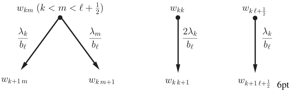
Figure 1. Vertices and edges.

Figure 1. Vertices and edges.

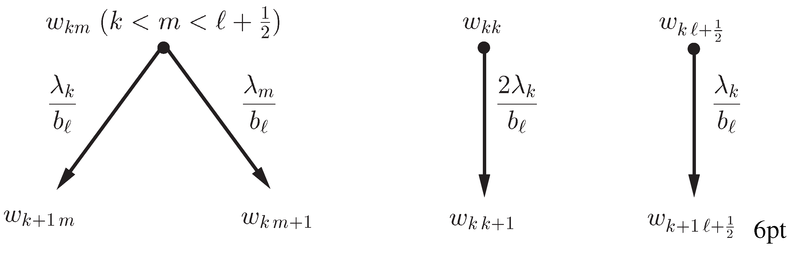
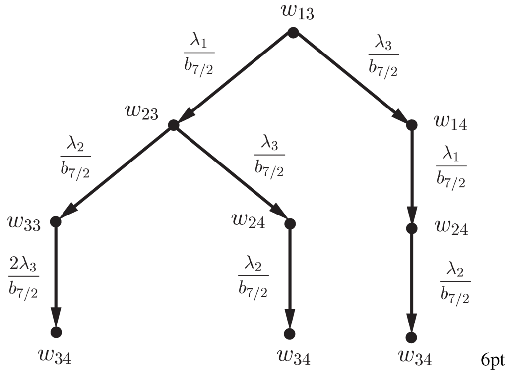
Figure 2. Example of rooted tree: $\ell =\frac{7}{2}$.

Figure 2. Example of rooted tree: $\ell =\frac{7}{2}$.

Proof of Lemma 8. The lemma is proved by induction on height of the trees. We have a tree of height zero only when label of the root is $w_{\ell -\frac{1}{2}\ell +\frac{1}{2}}.$ In this case no $c_{ab}$ appears so that Equation (52) yields

$$w_{\ell -\frac{1}{2}\ell +\frac{1}{2}}={\varphi }_{\ell -\frac{1}{2}\ell +\frac{1}{2}}-\gamma \left(\ell -\frac{1}{2},\ell +\frac{1}{2}\right)\frac{{\varphi }_{\ell +\frac{1}{2}\ell +\frac{1}{2}}^2}{2}$$

This coincide with Equation (50). To verify the legitimacy of the algorithm calculating $c_{ab}(k,m)$ we need to start with a tree of height one. There are two possible labels of the root to obtain a tree of height one. They are $w_{\ell -\frac{3}{2}\ell +\frac{1}{2}}$ and $w_{\ell -\frac{1}{2}\ell -\frac{1}{2}}.$ Let us start with the label $w_{\ell -\frac{3}{2}\ell +\frac{1}{2}}$

It is not difficult to verify, by employing the algorithm, that we obtain the Equation (51) for this case. For the label $w_{\ell -\frac{1}{2}\ell -\frac{1}{2}},$ the algorithm gives the following result:

$$w_{\ell -\frac{1}{2}\ell -\frac{1}{2}}={\varphi }_{\ell -\frac{1}{2}\ell -\frac{1}{2}}-\frac{2{\lambda }_{\ell -\frac{1}{2}}}{b_{\ell }}{w}_{\ell -\frac{1}{2}\ell +\frac{1}{2}}{\varphi }_{\ell +\frac{1}{2}\ell +\frac{1}{2}}-2{\left(\frac{2{\lambda }_{\ell -\frac{1}{2}}}{b_{\ell }}\right)}^2\frac{{\varphi }_{\ell +\frac{1}{2}\ell +\frac{1}{2}}^3}{3!}$$

(54)

It is easy to see that $\tilde{C}$ annihilates Equation (54). Thus the lemma is true for trees of height one.

Now we consider trees of height $h>1.$ If label of the root is $w_{km}(k<m<\ell +\frac{1}{2}),$ then the tree has two rooted subtrees (height $h-1$) such that one of then has the root whose label is $w_{k+1m}$ and another has the root whose label is $w_{km+1}.$ On the other hand, if label of the root is $w_{kk}$ or $w_{k\ell +\frac{1}{2}},$ then the tree has only one rooted subtree (height $h-1$) such that the subtree has the root whose label is $w_{kk+1}$ or $w_{k+1\ell +\frac{1}{2}}.$ By the algorithm one may find relations between the coefficients $c_{ab},\gamma$ for the tree of height h and the subtrees of height $h-1:$

$$\begin{array}{ccc}\hfill c_{ab}(k,m)& =& \frac{{\lambda }_k}{b_{\ell }}{c}_{a-1b}(k+1,m)+\frac{{\lambda }_m}{b_{\ell }}{c}_{ab-1}(k,m+1),\hfill \end{array}$$

$$\begin{array}{ccc}\hfill \gamma (k,m)& =& \frac{{\lambda }_k}{b_{\ell }}\gamma (k+1,m)+\frac{{\lambda }_m}{b_{\ell }}\gamma (k,m+1),\hfill \end{array}$$

$$\begin{array}{ccc}\hfill c_{ab}(k,k)& =& \frac{2{\lambda }_k}{b_{\ell }}{c}_{ab-1}(k,k+1),\gamma (k,k)=\frac{2{\lambda }_k}{b_{\ell }}\gamma (k,k+1)\hfill \end{array}$$

(55)

We understand that $c_{ab}$ and γ are zero if their indices or arguments have a impossible value.

Assumption of the induction is that the lemma is true for any rooted subtrees whose height is smaller than $h.$ Namely, we assume that $\tilde{C}{w}_{k+am+b}=0$ for $a+b\ge 1$ and what we need to show is that $\tilde{C}{w}_{km}=0.$ We separate out $a+b=1$ terms from the summation in Equation (52) and use Equation (46) to calculate the action of $\tilde{C}$ on $w_{km}.$ For $k<m<\ell +\frac{1}{2}$ we have

$$\begin{array}{ccc}\hfill \tilde{C}{w}_{km}& =& \tilde{C}{\varphi }_{km}-{\lambda }_k{w}_{k+1m}-{\lambda }_m{w}_{km+1}\hfill \\ & -& b_{\ell }\sum _{a+b\ge 2}{c}_{ab}(k,m)w_{k+am+b}\frac{{\varphi }_{\ell +\frac{1}{2}\ell +\frac{1}{2}}^{a+b-1}}{(a+b-1)!}-b_{\ell }\gamma (k,m)\frac{{\varphi }_{\ell +\frac{1}{2}\ell +\frac{1}{2}}^{2\ell +1-k-m}}{(2\ell +1-k-m)!}\hfill \\ & =& \tilde{C}{\varphi }_{km}-{\lambda }_k{w}_{k+1m}-{\lambda }_m{w}_{km+1}\hfill \\ & -& \sum _{a+b\ge 1}\left({\lambda }_k{c}_{ab}(k+1,m)w_{k+1+am+b}+{\lambda }_m{c}_{ab}(k,m+1)w_{km+1}\right)\frac{{\varphi }_{\ell +\frac{1}{2}\ell +\frac{1}{2}}^{a+b}}{(a+b)!}\hfill \\ & -& \left({\lambda }_k\gamma (k+1,m)+{\lambda }_m\gamma (k,m+1)\right)\frac{{\varphi }_{\ell +\frac{1}{2}\ell +\frac{1}{2}}^{2\ell +1-k-m}}{(2\ell +1-k-m)!}\hfill \end{array}$$

The second equality is due to the relations Equation (55) and the replacement $a-1$ (resp. $b-1$) with a (resp. b). By the assumption of the induction one may use Equation (52) to obtain:

$$\tilde{C}{w}_{km}=\tilde{C}{\varphi }_{km}-({\lambda }_k{\varphi }_{k+1m}+{\lambda }_m{\varphi }_{km+1})=0$$

The second equality is due to Equation (46).

The proof of $\tilde{C}{w}_{kk}=\tilde{C}{w}_{k\ell +\frac{1}{2}}=0$ is done in a similar way. This completes the proof of Lemma 8.  □

Corollary 9. The variables $w_{k\ell +\frac{1}{2}}(1\le k\le \ell -\frac{1}{2})$ are easily calculated by this method.

$$w_{k\ell +\frac{1}{2}}={\varphi }_{k\ell +\frac{1}{2}}-\sum _{n=1}^{\ell -\frac{1}{2}-k}\left(\begin{array}{c}2\ell +1-k\\ n\end{array}\right)w_{k+n\ell +\frac{1}{2}}{\left(\frac{{\varphi }_{\ell +\frac{1}{2}\ell +\frac{1}{2}}}{b_{\ell }}\right)}^n-\left(\begin{array}{c}2\ell +1-k\\ \ell +\frac{1}{2}\end{array}\right)\frac{1}{b_{\ell }^{\ell +\frac{1}{2}-k}}\frac{{\varphi }_{\ell +\frac{1}{2}\ell +\frac{1}{2}}^{\ell +\frac{3}{2}-k}}{\ell +\frac{3}{2}-k}$$

Proof of Corollary 9. The rooted tree used for this computation is indicated in Figure 3. It follows that the coefficient of $w_{k+a\ell +\frac{1}{2}}$ is given by

$$c_{a0}(k,\ell +\frac{1}{2})=\frac{{\lambda }_k{\lambda }_{k+1}\dots {\lambda }_{k+a-1}}{b_{\ell }^a}=\left(\begin{array}{c}2\ell +1-k\\ a\end{array}\right)\frac{a!}{b_{\ell }^a}$$

By Equation (53) the coefficient $\gamma (k,\ell +\frac{1}{2})$ is calculated as $\gamma (k,\ell +\frac{1}{2})={\lambda }_{\ell -\frac{1}{2}}{b}_{\ell }^{-1}{c}_{\ell -\frac{1}{2}-k0}(k,\ell +\frac{1}{2}).$ Thus we obtain the expression of $w_{k\ell +\frac{1}{2}}$ given in the corollary.   □

Figure 3. Rooted tree for the computation of $w_{k\ell +\frac{1}{2}}$.

Figure 3. Rooted tree for the computation of $w_{k\ell +\frac{1}{2}}$.

Our final task is to consider the invariance under $D.$ It is immediate to see that $\widehat{D}$ scales $w_{km}$ as

$$w_{km}\to e^{-2(2\ell +2-k-m)ϵ}{w}_{km}$$

Together with the scaling law Equation (44) we arrive at the final theorem.

Theorem 10. The PDE invariant under the group generated by ${\mathfrak{g}}_{\ell }$ with $\ell \ge \frac{5}{2}$ is given by

$$F\left(\frac{w_{km}}{w^{2\ell +2-k-m}}\right)=0,1\le k\le \ell -\frac{1}{2},k\le m\le \ell +\frac{1}{2}$$

(56)

where F is an arbitrary differentiable function. The variables w and $w_{km}$ are given in Equations (41) and (52), respectively. This is the PDE with $\ell +\frac{3}{2}$ independent and one dependent variables. The function F has $\frac{1}{2}\left(\ell -\frac{1}{2}\right)\left(\ell +\frac{5}{2}\right)$ arguments.

Example 1. Invariant PDE for $\ell =\frac{5}{2}.$

$$F\left(\frac{w_{11}}{w^5},\frac{w_{12}}{w^4},\frac{w_{13}}{w^3},\frac{w_{22}}{w^3},\frac{w_{23}}{w^2}\right)=0$$

where

$$\begin{array}{ccc}\hfill w& =& \frac{U_0}{U}+x_2\frac{U_1}{U}+2x_3\frac{U_2}{U}-\frac{U_3^2}{8U^2},\hfill \\ \hfill w_{23}& =& {\varphi }_{23}-\frac{1}{18}{\varphi }_{33}^2,\hfill \\ \hfill w_{22}& =& {\varphi }_{22}-\frac{2}{9}{\varphi }_{23}{\varphi }_{33}+\frac{2}{3^5}{\varphi }_{33}^3,\hfill \\ \hfill w_{13}& =& {\varphi }_{13}-\frac{5}{36}{\varphi }_{23}{\varphi }_{33}+\frac{5}{2^2{3}^5}{\varphi }_{33}^3,\hfill \\ \hfill w_{12}& =& {\varphi }_{12}-\frac{1}{9}{\varphi }_{13}{\varphi }_{33}-\frac{5}{36}{\varphi }_{22}{\varphi }_{33}+\frac{5}{2^3{3}^3}{\varphi }_{23}{\varphi }_{33}^2-\frac{5}{2^5{3}^5}{\varphi }_{33}^4,\hfill \\ \hfill w_{11}& =& {\varphi }_{11}-\frac{5}{18}{\varphi }_{12}{\varphi }_{33}+\frac{5}{2^2{3}^4}{\varphi }_{13}{\varphi }_{33}^2-\frac{25}{2^4{3}^4}{\varphi }_{22}{\varphi }_{33}^2-\frac{25}{2^4{3}^6}{\varphi }_{23}{\varphi }_{33}^3-\frac{5}{2^4{3}^8}{\varphi }_{33}^5\hfill \end{array}$$

The symmetry generators are given by

$$\begin{array}{c}M=U{\partial }_U,D=2t{\partial }_t+5x_1{\partial }_{x_1}+3x_2{\partial }_{x_2}+x_3{\partial }_{x_3},H={\partial }_t,\hfill \\ C=t(t{\partial }_t+5x_1{\partial }_{x_1}+3x_2{\partial }_{x_2}+x_3{\partial }_{x_3})+5x_1{\partial }_{x_2}+4x_2{\partial }_{x_3}-18x_3^{2}U{\partial }_U,\hfill \\ P^{\left(1\right)}={\partial }_{x_1},P^{\left(2\right)}=t{\partial }_{x_1}+{\partial }_{x_2},P^{\left(3\right)}=t^2{\partial }_{x_1}+2t{\partial }_{x_2}+{\partial }_{x_3},\hfill \\ P^{\left(4\right)}=t^3{\partial }_{x_1}+3t^2{\partial }_{x_2}+3t{\partial }_{x_3}-12x_{3}U{\partial }_U,\hfill \\ P^{\left(5\right)}=t^4{\partial }_{x_1}+4t^3{\partial }_{x_2}+4t^2{\partial }_{x_3}-24(2t{x}_3+x_2)U{\partial }_U,\hfill \\ P^{\left(6\right)}=t^5{\partial }_{x_1}+5t^4{\partial }_{x_2}+10t^3{\partial }_{x_3}-120(t^2{x}_3-t{x}_2+x_1)U{\partial }_U\hfill \end{array}$$

6. Concluding Remarks

We have constructed nonlinear PDEs invariant under the transformations generated by the realization of CGA given in Equation (2). This was done by obtaining the general solution of the symmetry conditions so that the PDEs constructed in this work are the most general ones invariant under Equation (2). A remarkable property of the PDEs is that they do not contain the second order derivative in t if $\ell >\frac{3}{2}.$ It means that there exist no invariant PDEs of wave or Klein–Gordon type for $\ell >\frac{3}{2}.$ This type of ℓ-dependence does not appear in the linear PDEs constructed in [1,4] based on the representation theory of ${\mathfrak{g}}_{\ell }.$ This will be changed if one start with a realization of CGA which is different from Equation (2).

The CGAs considered in this work are only $d=1$ members. Extending the present computation to higher values of d would be an interesting future work. Because the $d=2$ CGA has a distinct central extension so that we will have different types of invariant PDEs. For $d\ge 3$ CGAs have $so\left(d\right)$ as a subalgebra. This will also cause a significant change in invariant PDEs.

References

- Aizawa, N.; Kimura, Y.; Segar, J. Intertwining operators for ℓ-conformal Galilei algebras and hierarchy of invariant equations. J. Phys. A Math. Theor. 2013, 46. [Google Scholar] [CrossRef]
- Aizawa, N.; Dobrev, V.K.; Doebner, H.D. Intertwining operators for Schrödinger algebras and hierarchy of invariant equations. In Quantum Theory and Symmetries; Kapuścik, E., Horzela, A., Eds.; World Scientific: Singapore, 2002; pp. 222–227. [Google Scholar]
- Aizawa, N.; Dobrev, V.K.; Doebner, H.D.; Stoimenov, S. Intertwining operators for the Schrödinger algebra in n ≥ 3 space dimension. In Proceedings of the VII International Workshop on Lie Theory and Its Applications in Physics; Doebner, H.D., Dobrev, V.K., Eds.; Heron Press: Sofia, Bulgaria, 2008; pp. 372–399. [Google Scholar]
- Aizawa, N.; Chandrashekar, R.; Segar, J. Lowest weight representations, singular vectors and invariant equations for a class of conformal Galilei algebras. SIGMA 2015, 11. [Google Scholar] [CrossRef]
- Negro, J.; del Olmo, M.; Rodrıguez-Marco, A. Nonrelativistic conformal groups. J. Math. Phys. 1997, 38, 3786–3809. [Google Scholar] [CrossRef]
- Negro, J.; del Olmo, M.; Rodrıguez-Marco, A. Nonrelativistic conformal groups. II. Further developments and physical applications. J. Math. Phys. 1997, 38, 3810–3831. [Google Scholar] [CrossRef]
- Havas, P.; Plebański, J. Conformal extensions of the Galilei group and their relation to the Schrödinger group. J. Math. Phys. 1978, 19, 482–488. [Google Scholar] [CrossRef]
- Henkel, M. Local scale invariance and strongly anisotropic equilibrium critical systems. Phys. Rev. Lett. 1997, 78. [Google Scholar] [CrossRef]
- Martelli, D.; Tachikawa, Y. Comments on Galilean conformal field theories and their geometric realization. JHEP 2010, 5, 1–31. [Google Scholar] [CrossRef]
- Lie, S. Theorie der Transformationsgruppen; Chelsea: New York, NY, USA, 1970. [Google Scholar]
- Jacobi, C.G.J.; Borchardt, C.W. Vorlesungen über Dynamik; Reimer, G., Ed.; University of Michigan Library: Ann Arbor, MI, USA, 1866. [Google Scholar]
- Niederer, U. The maximal kinematical invariance group of the free Schrodinger equation. Helv. Phys. Acta 1972, 45, 802–810. [Google Scholar]
- Niederer, U. The maximal kinematical invariance group of the harmonic oscillator. Helv. Phys. Acta 1973, 46, 191–200. [Google Scholar]
- Niederer, U. The maximal kinematical invariance groups of schroedinger equations with arbitrary potentials. Helv. Phys. Acta 1974, 47, 167–172. [Google Scholar]
- Hagen, C.R. Scale and conformal transformations in Galilean-covariant field theory. Phys. Rev. D 1972, 5, 377–388. [Google Scholar] [CrossRef]
- Jackiw, R. Introducing scale symmetry. Phys. Today 1972, 25, 23–27. [Google Scholar] [CrossRef]
- Burdet, G.; Perrin, M. Many-body realization of the Schrödinger algebra. Lett. Nuovo Cim. 1972, 4, 651–655. [Google Scholar] [CrossRef]
- Son, D.T. Toward an AdS/cold atoms correspondence: A geometric realization of the Schroedinger symmetry. Phys. Rev. D 2008, 78. [Google Scholar] [CrossRef]
- Balasubramanian, K.; McGreevy, J. Gravity duals for nonrelativistic conformal field theories. Phys. Rev. Lett. 2008, 101. [Google Scholar] [CrossRef]
- Unterberger, J.; Roger, C. The Schrödinger-Virasoro Algebra: Mathematical Structure and Dynamical Schrödinger Symmetries; Springer: Berlin/Heidelberg, Germany, 2012. [Google Scholar]
- Aizawa, N.; Isaac, P.S.; Kimura, Y. Highest weight representations and Kac determinants for a class of conformal Galilei algebras with central extension. Int. J. Math. 2012, 23, 1250118:1–1250118:25. [Google Scholar] [CrossRef]
- Henkel, M. Phenomenology of local scale invariance: From conformal invariance to dynamical scaling. Nucl. Phys. B 2002, 641, 405–486. [Google Scholar] [CrossRef]
- Aizawa, N.; Isaac, P.S. On irreducible representations of the exotic conformal Galilei algebra. J. Phys. A Math. Theor. 2011, 44. [Google Scholar] [CrossRef]
- Lü, R.; Mazorchuk, V.; Zhao, K. On simple modules over conformal Galilei algebras. J. Pure Appl. Algebra 2014, 218, 1885–1899. [Google Scholar] [CrossRef]
- Fushchich, W.I.; Cherniha, R.M. The Galilean relativistic principle and nonlinear partial differential equations. J. Phys. A Math. Gen. 1985, 18, 3491–3503. [Google Scholar] [CrossRef]
- Fushchich, W.I.; Cherniha, R.M. Galilei invariant non-linear equations of Schrödinger type and their exact solutions. I. Ukr. Math. J. 1989, 41, 1161–1167. [Google Scholar] [CrossRef]
- Rideau, G.; Winternitz, P. Evolution equations invariant under two-dimensional space-time Schrödinger group. J. Math. Phys. 1993, 34, 558–570. [Google Scholar] [CrossRef]
- Cherniha, R.M.; Henkel, M. The exotic conformal Galilei algebra and nonlinear partial differential equations. J. Math. Anal. Appl. 2010, 369, 120–132. [Google Scholar] [CrossRef]
- Fushchych, W.I.; Cherniha, R.M. Galilei-invariant nonlinear systems of evolution equations. J. Phys. A Math. Gen. 1995, 28, 5569–5579. [Google Scholar] [CrossRef]
- Cherniha, R.M.; Henkel, M. On non-linear partial differential equations with an infinite-dimensional conditional symmetry. J. Math. Anal. Appl. 2004, 298, 487–500. [Google Scholar] [CrossRef]
- Duval, C.; Horvathy, P.A. Non-relativistic conformal symmetries and Newton–Cartan structures. J. Phys. A Math. Theor. 2009, 42. [Google Scholar] [CrossRef]
- Duval, C.; Horvathy, P.A. Conformal Galilei groups, Veronese curves and Newton–Hooke spacetimes. J. Phys. A Math. Theor. 2011, 44, 335203:1–335203:21. [Google Scholar] [CrossRef]
- Gomis, J.; Kamimura, K. Schrödinger equations for higher order nonrelativistic particles and N-Galilean conformal symmetry. Phys. Rev. D 2012, 85. [Google Scholar] [CrossRef]
- Galajinsky, A.; Masterov, I. Remarks on l-conformal extension of the Newton–Hooke algebra. Phys. Lett. B 2011, 702, 265–267. [Google Scholar] [CrossRef]
- Galajinsky, A.; Masterov, I. Dynamical realization of l-conformal Galilei algebra and oscillators. Nucl. Phys. B 2013, 866, 212–227. [Google Scholar] [CrossRef] [Green Version]
- Galajinsky, A.; Masterov, I. Dynamical realizations of l-conformal Newton–Hooke group. Phys. Lett. B 2013, 723, 190–195. [Google Scholar] [CrossRef]
- Andrzejewski, K.; Galajinsky, A.; Gonera, J.; Masterov, I. Conformal Newton–Hooke symmetry of Pais–Uhlenbeck oscillator. Nucl. Phys. B 2014, 885, 150–162. [Google Scholar] [CrossRef]
- Galajinsky, A.; Masterov, I. On dynamical realizations of l-conformal Galilei and Newton–Hooke algebras. Nucl. Phys. B 2015, 896, 244–254. [Google Scholar] [CrossRef]
- Andrzejewski, K.; Gonera, J.; Kosiński, P.; Maślanka, P. On dynamical realizations of l-conformal Galilei groups. Nucl. Phys. B 2013, 876, 309–321. [Google Scholar] [CrossRef] [Green Version]
- Andrzejewski, K.; Gonera, J.; Kijanka-Dec, A. Nonrelativistic conformal transformations in Lagrangian formalism. Phys. Rev. D 2013, 87. [Google Scholar] [CrossRef]
- Andrzejewski, K.; Gonera, J. Dynamical interpretation of nonrelativistic conformal groups. Phys. Lett. B 2013, 721, 319–322. [Google Scholar] [CrossRef]
- Andrzejewski, K.; Gonera, J. Unitary representations of N-conformal Galilei group. Phys. Rev. D 2013, 88. [Google Scholar] [CrossRef]
- Andrzejewski, K. Conformal Newton–Hooke algebras, Niederer’s transformation and Pais–Uhlenbeck oscillator. Phys. Lett. B 2014, 738, 405–411. [Google Scholar] [CrossRef]
- Andrzejewski, K.; Gonera, J.; Maślanka, P. Nonrelativistic conformal groups and their dynamical realizations. Phys. Rev. D 2012, 86. [Google Scholar] [CrossRef]
- Aizawa, N.; Kuznetsova, Z.; Toppan, F. ℓ-oscillators from second-order invariant PDEs of the centrally extended Conformal Galilei Algebras. J. Math. Phys. 2015, 56, 031701:1–031701:14. [Google Scholar] [CrossRef]
- Olver, P. Applications of Lie Groups to Differential Equations; Springer: New York, NY, USA, 2000. [Google Scholar]
- Bluman, G.W.; Kumei, S. Symmetries and Differential Equations; Springer: New York, NY, USA, 1989. [Google Scholar]
- Stephani, H. Differential Equations: Their Solution Using Symmetries; Cambridge University Press: New York, NY, USA, 1989. [Google Scholar]
- Courant, R.; Hilbert, D. Methods of Mathematical Physics; CUP Archive: New York, NY, USA, 1966; Volume 1. [Google Scholar]
© 2015 by the authors; licensee MDPI, Basel, Switzerland. This article is an open access article distributed under the terms and conditions of the Creative Commons Attribution license (http://creativecommons.org/licenses/by/4.0/).