Abstract
In the field of mineral processing, an accurate image segmentation method is crucial for measuring the size distribution of run-of-mine ore on the conveyor belts in real time0The image-based measurement is considered to be real time, on-line, inexpensive, and non-intrusive. In this paper, a new belt ore image segmentation method was proposed based on a convolutional neural network and image processing technology. It consisted of a classification model and two segmentation algorithms. A total of 2880 images were collected as an original dataset from the process control system (PCS). The test images were processed using the proposed method, the PCS system, the coarse image segmentation (CIS) algorithm, and the fine image segmentation (FIS) algorithm, respectively. The segmentation results of each algorithm were compared with those of the manual segmentation. All empty belt images in the test images were accurately identified by our method. The maximum error between the segmentation results of our method and the results of manual segmentation is 5.61%. The proposed method can accurately identify the empty belt images and segment the coarse material images and mixed material images with high accuracy. Notably, it can be used as a brand new algorithm for belt ore image processing.
1. Introduction
The particle size distribution of run-of-mine ore exhibits a great influence on the grinding process. Variations in the particle size distribution directly affect the throughput and power consumption of mills, especially autogenous (AG) and semi-autogenous (SAG) grinding mills [1]. Therefore, it is critical to evaluate the size distribution of run-of-mine ore on the conveyor belts in real time [2,3]. The measurement of the particle size distribution by sampling and sieving is considered a common and time-consuming method. The analysis method based on machine vision is considered a non-invasive, fast, and inexpensive technique for rock size measurement [4]. Since the 1980s, many studies have been conducted to evaluate the particle size distribution of materials on a conveyor belt based on machine vision and image processing technology [2,5,6]. Scholars have mainly followed three aspects of exploration. The first aspect includes accurate ore contour detection algorithms. The second aspect is the reasonable evaluation model which is used to convert two-dimensional information of ore into three-dimensional information, and then evaluating energy consumption or particle size distribution. The third aspect is new technology including neural networks, deep learning, and genetic algorithms, etc. In 1988, Lange developed an on-line, real-time system which can capture images of rocks on conveyor belts, and process images to get the chord-length distributions, and then transform chord-length distributions to equivalent sieve sizes. Lange offered a method to distinguish belt ores of different size distributions [2]. Lin and Miller developed an image-based system which used image processing technology to get the chord-length of rocks, and used two kernel functions to calculate the cumulative chord-length distributions of regularly and irregular shaped particles, respectively. The last step was to transform the chord-length distributions into size distributions by the transformation Equation [5]. In 1997, Yen and co-workers used an empirical correction function to solve the coarse particle overlap problem [7]. Before 2000, limited by hardware technology, it was difficult to get sharp images and many algorithms that consumed too much computer performance could not be adopted. The scholars mainly researched the image-based system software and hardware framework, contour detection, reasonable measurement parameters and size transformation functions.
After 2000, with the rapid development of computer hardware and new technologies, the image-based, online, and real-time particle size measurement development made much progress. Singh and Mohan Rao extracted RGB color information, visual texture of particles, and developed a system based on a radial basis neural network. The system was used for ore classification and ore sorting [8]. Al-Thyabat and co-workers evaluated ore image segmentation results by means of Feret’s diameter and equivalent area diameter, and experimented and discussed the effect of camera positions [9]. Levner offered a classification-driven watershed segmentation to segment belt ore images, and adopted machine learning to produce markers and identify ore edges [10]. Outal et al. provided a calibration method for evaluating 3D size distribution, according to the 2D segmentation results [11]. Andersson evaluated the size distribution of particles using ordinal logistic regression [12]. Hamzeloo et al. used different particle equivalent models to evaluate 3D size distribution. These equivalent models included the equivalent area circle, best-fit rectangle, Feret diameter, and maximum inscribed disk [4]. In addition, the impact of the shape of the particles on the product properties was also researched extensively [13,14,15,16]. Until now, many image-based analysis methods have been successfully applied to evaluate the particle size distribution [17,18,19], however there are still three unresolved problems regarding the image-based, on-line particle size analysis methods.
One is that there is no research focus on the problem of empty belt identification. In the course of production, we should not turn on or switch to the empty conveyor belts. Therefore, the accurate recognition of the empty belt is necessary to realize the automatic control and switching of conveyor belts. The second problem is the accurate belt ore image segmentation method, especially for the coarse-fine images. According to the experimental results of previous researches, it cannot be concluded that the proposed method can accurately segment both coarse and fine materials. An accurate image segmentation method is the basis of a particle size distribution measurement system. Although there is a method which uses machine learning to identify the pixels of ore edges, the contour detection based on image segmentation is more stable, accurate, and adaptable. In the future, the ore image segmentation method based on deep learning will be an expected practice. The third problem is related to the overlapping of particles. Even though many studies have been conducted in order to find viable solutions to these problems, most of them rely on empirical correction [4,7,20]. Dynamic image analysis (DIA) is a feasible method to solve the overlap problem [15].
Traditional rock image analysis methods cannot distinguish different types of images, such as empty belt images, mixed material images, and coarse material images, which are distinct. The mixed materials include coarse-fine materials and fine materials. It is difficult to accurately process all three types of belt ore images with an image segmentation algorithm; therefore, our analysis method should be able to accurately classify the images we obtain. In recent years, with the rapid development of computer hardware and deep learning theory, the convolutional neural networks (CNNs) have shown great progress in the field of image recognition and classification [21,22]. Krizhevsky et al. developed AlexNet, which can reach 83.6% top-5 accuracy for the ImageNet dataset [23]. At present, the top-5 accuracy of many convolutional neural networks in image recognition tasks can reach more than 90% for the ImageNet dataset [24,25,26]. Many research studies on rock image recognition and classification based on deep learning have achieved high accuracy [8,27,28].
In this research, the method based on the deep learning method and the image processing technology was developed in order to accurately segment the belt ore images. The strategy was to classify the belt ore images into empty belt, mixed materials and coarse materials first and then use different algorithms for processing mixed materials and coarse materials. We focused on the accuracy of belt ore image segmentation and empty belt identification. Both the conversion model for converting two-dimensional information of ore into three-dimensional information and the impact of the shape of the particles on the product properties are beyond the scope of this article.
2. Details of the Method
The proposed method is divided into three layers. The first layer is a classifier based on a convolutional neural network. The second layer consists of two image processing algorithms based on the OpenCV library. The two algorithms are used to process coarse material images and mixed material images, respectively. The third layer is the statistics layer. The classifier divides the raw images into the empty belt, coarse materials, and mixed materials. If the belt is empty, it gives an alarm; otherwise, it uses the coarse image segmentation (CIS) algorithm to process coarse material images and uses the fine image segmentation (FIS) algorithm to process mixed material images, respectively. Finally, the cumulative area distribution is calculated following the counting segmentation area information. The technical roadmap is shown in Figure 1.

Figure 1.
The technical roadmap of the method.
2.1. The Convolutional Neural Network Classifier
2.1.1. The Dataset Preparation
The size of the dataset is considered crucial for evaluating the performance of the trained model. An insufficient dataset causes a low recognition accuracy of the trained model. The dataset used in this study consisted of 2880 images collected from the process control system (PCS) system of a mineral-processing plant in the Yunnan Province, China. The images were taken by eight cameras installed on eight feeding belts with a collection rate of eight photos per minute for each camera. AXIS P3227-LVE cameras from AXIS are used, as well as LED PCS6-LED80 W lamps from Woodgrove. Two belt ore images are taken by each camera continuously every 15 s. The PCS system stores the latest 100 pictures from each camera; therefore, the images in the PCS system are completely updated every 12.5 min. We wrote a Python script to transfer the pictures from the storage folders to specified folders, and the transfer was executed every 13 min, lasting for a week. In the image transfer stage, the goal is to obtain sufficient belt ore images. It is efficient and economical to directly transfer images saved by the PCS system. At the same time, only two feeding belts are in running; therefore, there are a lot of duplicate images in the specified folders. All of the images have a size of 2304 × 1728 px (JPEG file). We planned to select about 3000 sharp, non-repetitive, and representative belt ore images as the original dataset. The 982 empty belt images were picked out including empty belts with water stains, empty belts with small particles, images taken by telephoto lens, and images taken by short focal length lens. We divided the belt ore images with fine content less than 30% into coarse material images. The features of coarse material images are obvious and similar; therefore, the number of coarse material images can be reduced appropriately. The 841 coarse material images were selected. The 1057 mixed material images were selected according to the proportion of fine material. The mixed material images were selected consisting of 100%, 90%, 70%, and 50% fine material. All images were taken from an industrial site and were not created; therefore, the proportion of fine material was an estimation and not an exact value. The 2880 high-quality, representative images were selected from the saved images as the original dataset. After physical verification, 522 px in each image was found to be equal to 30 cm. Several examples of the images are shown in Figure 2.
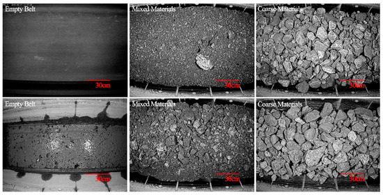
Figure 2.
Samples of the original dataset: empty belt, mixed materials, and coarse materials.
2.1.2. Model Training
The design of our network is shown in Figure 3. The network consists of two convolution layers, two maxpool layers, two fully connected layers, and three ReLU activation functions. The DELL R730 server was used to train the model. The Windows Server 2012 was used as the operating system. The Intel E5–2609V4 was used as the CPU with a RAM of 32 GB, and the Nvidia P2000 (5 GB) was used as the GPU.
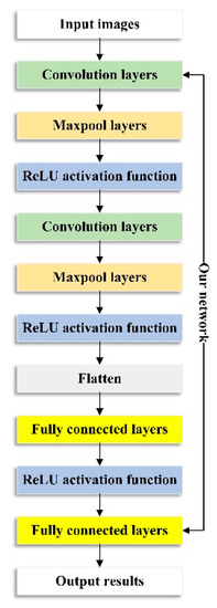
Figure 3.
The architecture of our network.
The original dataset was used as the raw data. The input images consisted of three channels, which were resized to 500 × 500 × 3. All input images were required to undergo a two-step pretreatment process. In the first step, the value range of pixels was changed from 0–255 to 0–1. In the second step, the image was normalized by using the empirical mean vector and the empirical std vector. The normalization is described as follows:
The original dataset was completely shuffled: 20% of the images assigned to the test set, 20% of the images assigned to the validation set, and 60% of the images used as the training set. The processed images were input into the neural network for model training. The epoch value was set to 10, the batch size was set to 32, the learning rate was set to 0.001, and the cross-entropy was used to evaluate the training loss. The prediction result was compared with the true label in order to calculate the training accuracy and the validation accuracy of every epoch. The training accuracy and validation accuracy were used to update the weights in the model [29]. The training process is shown in Figure 4. The training accuracy was 99.48%, the validation accuracy was 100%, and the training cross-entropy equaled 0.0146 when the epoch equaled 10. The model was tested with the test set, and the prediction accuracy was 100%.
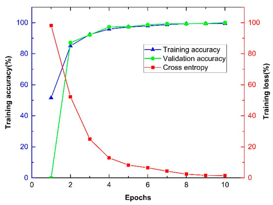
Figure 4.
Training process using our network.
2.2. CIS and FIS Algorithms
2.2.1. CIS Algorithm
The CIS algorithm processes images classified by the classifier as coarse materials. The CIS algorithm is based on the Python OpenCV library (version 4.1.1). The uneven color distribution on the surface of the coarse ores and the coarse ores covered by fine particles led to the region of coarse ores in the image being divided into many small regions. Therefore, the CIS algorithm should be able to remove features that are similar to the ore edge on the surface of the coarse ore. The CIS algorithm is described in Figure 5.

Figure 5.
Block diagram of the coarse image segmentation (CIS) algorithm.
The CIS algorithm follows five steps. In the first step, the input image is processed using the bilateralFilter function. The setting value of the diameter of each pixel neighborhood equals 25, the sigma parameter of the color space equals 100, and the sigma parameter of the coordinate space equals 25. The purpose of bilateral filtering is to blur the surface of coarse materials while preserving the edge. The parameters of the bilateralFilter function were chosen according to experience and practice; for example, 25, 50, 75, 100. After bilateral filtering, the noise, details, and small color blocks on the surface of the ore are blurred, and the edge of the ore is preserved [30,31]. In the second step, the operations include graying [32], adaptive thresholding [33], and median filtering [34,35]. The setting kernel of the median filter equals 3. The kernel of the median filter should not be too high, to prevent edge interruption. After several tries, the results processed using the kernel with a value of 3 was more suitable for subsequent processing than 5 or 7. After the second step, the color image is binarized and denoised. In the third step, the image is processed using the findContours and drawContours functions. After these operations, the interconnected areas are closed. In the fourth step, the image is processed using the erode and morphologyEx functions [36,37,38]. The setting kernel is a 3 × 3 morph ellipse. The iterations parameter of the erode function is 10 and the iterations parameter of the morphologyEx function is 4. The target of erosion and open operation is to extract markers. The iterations parameters are sensitive, and are chosen by experience and trials. Finally, the watershed transformation is performed based on markers, and the watershed lines are drawn [10,39,40]. For instance, Figure 6 shows how the CIS algorithm processes a coarse material image.
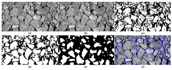
Figure 6.
Original (a), after the first step (b), after the second step (c), after the third step (d), after the fourth step (e), and after the fifth step (f).
2.2.2. FIS Algorithm
The FIS algorithm processes the images classified by the classifier as mixed materials. The FIS algorithm is based on the Python OpenCV library (version 4.1.1). Both fine and coarse-fine materials are mixed materials. The edge of fine materials is weak; therefore, excessive blurring causes the under-segmentation of fine material images, and insufficient blurring causes the over-segmentation of coarse material images. The FIS algorithm must remove the edge-like features on the surface of coarse ores as much as possible while retaining the outlines of granular particles and fine material. The FIS algorithm is described in Figure 7.
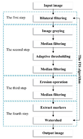
Figure 7.
Block diagram of the fine image segmentation (FIS) algorithm.
The FIS algorithm follows four steps. In the first step, the input image is processed using the bilateralFilter function. Due to the need to deal with the coarse ores which are contained in the mixed materials, it is necessary to use bilateral filtering. Parameter settings are found to be the same as the CIS algorithm [30,31]. In the second step, the operations include graying [32], adaptive thresholding [33], and two median filterings [34,35]. The setting kernels of the median filters equal 3. After the second step, the color image is binarized and denoised. In the third step, the image is processed using the erode function and median filtering. The setting kernel of the median filter equals 9 and the kernel of the erosion operation is a 5 × 5 morph ellipse [38]. Due to the edge of fine materials being weak, we should not adopt strong morphological operations. Therefore, the iterations were set to one. To ensure complete separation among markers, the kernel of the median filter in the third step was set to 9. Finally, the watershed transformation was performed based on markers and the watershed lines were drawn [10,40]. A mixed material image was processed using the FIS algorithm as shown in Figure 8.
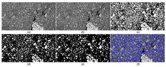
Figure 8.
Original (a), after the first step (b), after the second step (c), after the erosion operation (d), after the third step (e), and after the fourth step (f).
3. Experimental Details
3.1. Image Acquisition and Classification
The experimental dataset covers 12 representative images which consist of four empty belt images labelled as one, four mixed material images labelled as two, and four coarse material images labelled as zero. All images were taken from the PCS system at different times. We selected four empty belt images including an empty belt with water stains, an empty belt with small particles, an image taken by a telephoto lens, and an image taken by a short focal length lens. The features of coarse material images are obvious and similar. The four coarse material images were selected randomly. The four mixed material images were selected consisting of 100%, 90%, 70%, and 50% fine material. The raw images were divided into the following four groups: one empty belt image, one mixed material image, and one coarse material image in each group. In order to compare the segmentation results of the different algorithms, the designated region of raw images was processed by using different algorithms. The size of the designated region was 1202 × 631 (JPEG file). Manual segmentation was used to obtain accurate segmentation images. Images from group one (as shown in Figure 9a) were processed using PCS, CIS, and FIS, respectively, for evaluating each algorithm. Other images were processed and evaluated by using our method.

Figure 9.
The segmentation results processed by different algorithms: the original images (a), manual segmentation (b), process control system (PCS) (c), CIS (d), and FIS (e).
3.2. Estimation of Segmentation Accuracy
The area (px) of the regions surrounded by contours in the segmented images were counted, and the cumulative area distribution was calculated. Suppose , , …, are areas of the regions enclosed by the particle segmentation contours in a processed image. Among , , …, , areas of the regions that are smaller than the specified values are , , …, . The cumulative area distribution () is computed using the following equation:
We use the cumulative area distribution to evaluate the segmentation accuracy of algorithms. The specified value used to calculate the cumulative area distribution is called the area filter (px). If the number of pixels in the region surrounded by the contour is less than the area filter, the region can pass the area filter; otherwise, the region cannot pass. The contourArea function from the Python OpenCV library (version 4.1.1) was adopted to get the number of pixels in the region surrounded by the contour. The cumulative area distributions of the segmentation results of the empty belt image, mixed material image, and coarse material image are quite different; therefore, different area filters were used for calculating the cumulative area distribution of the segmented images. The empty belt images were evaluated using 2000, 4000, 8000, 10,000, 20,000, 40,000, 80,000, and 100,000 px area filters. The mixed material images were evaluated using 2000, 4000, 6000, 8000, 10,000, 20,000, 30,000, and 40,000 px area filters. The coarse material images were evaluated using 5000, 10,000, 15,000, 20,000, 25,000, 30,000, 35,000, and 40,000 px area filters. The cumulative area distribution and the number of segmentation contours of the image segmented by the PCS system, CIS, and FIS, respectively, were compared with the segmentation result of the manual segmentation image. The segmentation result of the algorithm, which was close to the manual segmentation result, was evaluated as accurate.
4. Experimental Results and Discussions
4.1. The Segmentation Result Analysis of Different Algorithms
Images in Figure 9a were segmented using manual segmentation, PCS, CIS, and FIS, respectively, providing results as shown in Figure 9b–e. By counting the number of segmentation contours in the segmented images, the results are shown in Table 1. By calculating the cumulative area distribution of the segmented images, the results are shown in Figure 10. Table 1 shows that the segmentation contour counts of the empty belt image by the PCS system, CIS algorithm and FIS algorithm, respectively, are 371, 51, 92. Figure 10a and Table 1 demonstrate that no algorithm can accurately segment the empty belt images. Due to many disturbing factors such as small particles, dirt, and water on the surface of the empty belts, the segmentation algorithms always segments the empty belt images. We only require to recognize and need not segment the empty belt images. Table 2 shows our method alarms all three empty belt images from groups 2 to 4. Table 2 indicates that using the training model based on the convolutional neural network to process the empty belt images shows better performance and accuracy. From Figure 10c and Table 1, it is observed that the PCS system shows serious over-segmentation in processing the coarse material images, and the segmentation accuracy of the FIS algorithm is found to be between that of the CIS algorithm and the PCS system. The outlines of massive rocks are obvious as compared to those of granular particles and fine material. Many disturbing factors, such as edges and corners, uneven color distribution, shadow, and so on, are found on the surface of massive rocks. An algorithm that can accurately segment the coarse material images must overcome the above interferences, however, the blur and denoise operations used cannot weaken the outlines of coarse ores too much. Figure 9 shows that the CIS algorithm has obvious advantages for segmenting the coarse material images. The blur, denoise, and smooth operations of the CIS algorithm weaken the outlines of ores; therefore, there is a serious under-segmentation in processing mixed material images, especially the fine material images (see Figure 9 and Figure 10b). We classified the images in the original dataset, which are neither coarse material images nor empty belt images, as mixed material images.

Table 1.
The segmentation contour count of various algorithms.
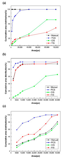
Figure 10.
The results of raw images by segmenting group 1 using manual segmentation, PCS, CIS, and FIS, respectively: empty belt (a), mixed materials (b), and coarse materials (c).

Table 2.
The results of empty belt images from groups 2 to 4, as processed by our method.
As the number of images in the original dataset is very high, it is not feasible to count the particle size distribution of materials on conveyor belts. The method of distinguishing empty, mixed materials, and coarse materials is based on artificial classification. An image that is full of massive ores is classified as a coarse material image. The accurate segmentation of mixed material images is most difficult to achieve. The massive ores show a greater impact on the grinding process. The results calculated by the under-segmentation of fine material images are found to be much coarser than the actual results. Fewer morphological operations enable the FIS algorithm to retain the outlines of granular particles and fine materials. More denoise operations enable the FIS algorithm to remove the interferences on the surface of the massive ores as much as possible. Figure 10b shows that the FIS algorithm shows accurate segmentation in processing mixed material images, especially the fine material images. As the FIS algorithm cannot remove the large non-edge features on the surface of massive rocks such as edges, corners, and color blocks, the FIS algorithm does not show as accurate results as the CIS algorithm in processing the coarse material images (see Figure 10c and Table 1). It is more accurate and reasonable to classify images first and then use different algorithms for processing rather than to process all images with the same algorithm.
4.2. The Processing Result Analysis of Our Method
Images from groups 2 to 4 were processed by using both our method and manual segmentation. Three mixed material images include one fine material image from group 2 and two mixed material images from groups 3 and 4. The results of the three processed empty belt images are shown in Table 2. The results of the three processed mixed material images are shown in Table 3. The results of the three processed coarse material images are shown in Table 4. The cumulative area distribution of one fine material image from group 2, one mixed material image from group 3, and one coarse material image from group 2, which were processed by our method, are shown in Figure 11. The column headers in Table 3 and Table 4 (5000, 10,000, etc.) indicate area filters. Table 2 shows that three empty belt images used for testing were alarmed. Our method is found to be accurate and reliable for empty belt identification. From Table 3, it is observed that the maximum error of the cumulative area distribution calculated by using different area filters is 2.71% for fine material, 4.65% for mixed materials from group 3, and 5.02% for mixed materials from group 4. From Table 3, the average error of the cumulative area distribution calculated by using different area filters is 1.07% for fine material, 2.27% for mixed materials from group 3, and 2.89% for mixed materials from group 4. From Table 4, it is observed that the maximum error of the cumulative area distribution calculated by using different area filters is 3.51%, 5.61%, 3.83%, respectively, for coarse materials from groups 2 to 4. From Table 4, the average error of the cumulative area distribution calculated by using different area filters is 1.30%, 3.30%, 2.59%, respectively, for coarse materials from groups 2 to 4. Table 3 and Table 4 indicate that our method can segment both mixed material images and coarse material images with high precision. Our method is considered useful for identifying and segmenting the images taken on industrial conveyor belts.

Table 3.
The results of mixed material images from groups 2 to 4, processed by our method.

Table 4.
The results of coarse material images from groups 2 to 4, processed by our method.

Figure 11.
The results of the specified images processed by our method: fine material (a), mixed materials (b), and coarse materials (c).
5. Conclusions
The objective of this study is to develop a method that can accurately segment belt ore images. The accurate image segmentation method is considered important for estimating the size distribution of mineral materials on industrial conveyor belts. For that purpose, 2880 images collected from a process control system on the industrial site were processed as the original dataset. Deep learning and image processing techniques were integrated with the image segmentation method. From the perspective of an application, the accurate recognition of the empty belts is necessary to realize the automatic switch of conveyor belts. The new method can identify the empty belt images with high precision. Moreover, it is difficult for an image segmentation algorithm to achieve accurate segmentation of both coarse materials and mixed materials. This study adopted the convolutional neural network model to solve the automatic classification of belt ore images, and then used the CIS algorithm and the FIS algorithm to accurately segment coarse material images and mixed material images, respectively. The new method makes it feasible and efficient to accurately process various belt ore images. Notably, it can be used as a brand new algorithm for belt ore image processing. The main novelties are as follows:
- This study used a convolutional neural network to identify empty belts.
- The new method adopted the strategy which is to classify the belt ore images first and then use different algorithms for processing different kinds of images.
Author Contributions
Conceptualization, X.M. (Xiqi Ma) and L.O.; methodology, X.M. (Xiqi Ma); software, X.M. (Xiqi Ma) and P.Z.; validation, X.M. (Xiqi Ma) and X.M. (Xiaofei Man); formal analysis, X.M. (Xiqi Ma) and P.Z.; investigation, X.M. (Xiqi Ma); resources, L.O.; data curation, X.M. (Xiqi Ma); writing—original draft preparation, X.M. (Xiqi Ma), X.M. (Xiaofei Man) and P.Z.; writing—review and editing, X.M. (Xiqi Ma), P.Z. and L.O.; supervision, L.O. All authors have read and agreed to the published version of the manuscript.
Funding
This work was financially supported by the National Natural Science Foundation of China (No. 51674291).
Acknowledgments
The authors also thank the support of the Key Laboratory of Hunan Province for Clean and Efficient Utilization of Strategic Calcium-containing Mineral Resources (No. 2018TP1002). Special thanks to Wencai Zhang for his suggestions on paper writing.
Conflicts of Interest
The authors declare no conflict of interest.
References
- Tessier, J.; Duchesne, C.; Bartolacci, G. A machine vision approach to on-line estimation of run-of-mine ore composition on conveyor belts. Miner. Eng. 2007, 20, 1129–1144. [Google Scholar] [CrossRef]
- Lange, T.B. Real-time measurement of the size distribution of rocks on a conveyor belt. IFAC Proc. Vol. 1988, 21, 25–34. [Google Scholar] [CrossRef]
- Ko, Y.D.; Shang, H. A neural network-based soft sensor for particle size distribution using image analysis. Powder Technol. 2011, 212, 359–366. [Google Scholar] [CrossRef]
- Hamzeloo, E.; Massinaei, M.; Mehrshad, N. Estimation of particle size distribution on an industrial conveyor belt using image analysis and neural networks. Powder Technol. 2014, 261, 185–190. [Google Scholar] [CrossRef]
- Lin, C.L.; Miller, J.D. Development of a pc, image-based, on-line particle-size analyzer. Min. Metall. Explor. 1993, 10, 29–35. [Google Scholar] [CrossRef]
- Liao, C.W.; Tarng, Y.S. On-line automatic optical inspection system for coarse particle size distribution. Powder Technol. 2009, 189, 508–513. [Google Scholar] [CrossRef]
- Yen, Y.K.; Lin, C.L.; Miller, J.D. Particle overlap and segregation problems in on-line coarse particle size measurement. Powder Technol. 1998, 98, 1–12. [Google Scholar] [CrossRef]
- Singh, V.; Rao, S.M. Application of image processing and radial basis neural network techniques for ore sorting and ore classification. Miner. Eng. 2005, 18, 1412–1420. [Google Scholar] [CrossRef]
- Al-Thyabat, S.; Miles, N.J.; Koh, T.S. Estimation of the size distribution of particles moving on a conveyor belt. Minerals Eng. 2007, 20, 72–83. [Google Scholar] [CrossRef]
- Ilya, L.; Hong, Z. Classification-driven watershed segmentation. IEEE Trans. Image Process. 2007, 16, 1437–1445. [Google Scholar]
- Outal, S.; Schleifer, J.; Pirard, E. In Evaluating a calibration method for the estimation of fragmented rock 3d-size-distribution out of 2d images. In Proceedings of the FRAGBLAST 9—9th International Symposium on Rock Fragmentation by Blasting, Granada, Spain, 13–17 September 2009; pp. 221–228. [Google Scholar]
- Andersson, T.; Thurley, M.J. Minimizing profile error when estimating the sieve-size distribution of iron ore pellets using ordinal logistic regression. Powder Technol. 2011, 206, 218–226. [Google Scholar] [CrossRef]
- Igathinathane, C.; Pordesimo, L.O.; Columbus, E.P.; Batchelor, W.D.; Methuku, S.R. Shape identification and particles size distribution from basic shape parameters using imagej. Comput. Electron. Agric. 2008, 63, 168–182. [Google Scholar] [CrossRef]
- Gawenda, T.; Krawczykowski, D.; Krawczykowska, A.; Saramak, A.; Nad, A. Application of dynamic analysis methods into assessment of geometric properties of chalcedonite aggregates obtained by means of gravitational upgrading operations. Minerals 2020, 10, 180. [Google Scholar] [CrossRef]
- Krawczykowski, D. Application of a vision systems for assessment of particle size and shape for mineral crushing products. IOP Conf. Ser. Mater. Sci. Eng. 2018, 427, 1–5. [Google Scholar] [CrossRef]
- Fannin, R.J.; Shuttle, D.A.; Rousé, P.C. Influence of roundness on the void ratio and strength of uniform sand. Géotechnique 2008, 58, 227–231. [Google Scholar]
- Split Engineering Products. Split-Online Software and Systems. 2020. Available online: https://www.spliteng.com/products/split-online-systems/ (accessed on 12 January 2020).
- Outotec Products and Services. Outotec® Act Grinding Optimization System. 2020. Available online: http://www.outotec.cn/products-and-services/technologies/grinding/act-grinding-optimization-system/ (accessed on 3 February 2020).
- WipWare Products and Services. Wipware Conveyor Analysis System. 2020. Available online: http://wipware.com/products/momentum/ (accessed on 7 January 2020).
- Zhang, Z.; Yang, J.; Ding, L.; Zhao, Y. Estimation of coal particle size distribution by image segmentation. Int. J. Mining Sci. Technol. 2012, 22, 739–744. [Google Scholar]
- Chauhan, R.; Ghanshala, K.K.; Joshi, R.C. Convolutional neural network (cnn) for image detection and recognition. In Proceedings of the 2018 First International Conference on Secure Cyber Computing and Communication (ICSCCC), Jalandhar, India, 15–17 December 2018. [Google Scholar]
- Sultana, F.; Sufian, A.; Dutta, P. Advancements in image classification using convolutional neural network. In Proceedings of the 2018 Fourth International Conference on Research in Computational Intelligence and Communication Networks (ICRCICN), Kolkata, India, 22–23 November 2018; IEEE: Piscataway, NJ, USA; pp. 122–129. [Google Scholar]
- Krizhevsky, A.; Sutskever, I.; Hinton, G.E. Imagenet classification with deep convolutional neural networks. Adv. Neural Inf. Process. Syst. 2012, 25. [Google Scholar] [CrossRef]
- He, K.; Zhang, X.; Ren, S.; Sun, J. Deep residual learning for image recognition. In Proceedings of the IEEE Conference on Computer Vision and Pattern Recognition, Las Vegas, NV, USA, 27–30 June 2016; pp. 770–778. [Google Scholar]
- Szegedy, C.; Liu, W.; Jia, Y.; Sermanet, P.; Reed, S.; Anguelov, D.; Erhan, D.; Vanhoucke, V.; Rabinovich, A. Going deeper with convolutions. In Proceedings of the IEEE Conference on Computer Vision and Pattern Recognition, Columbus, OH, USA, 23–28 June 2014. [Google Scholar]
- Simonyan, K.; Zisserman, A. Very deep convolutional networks for large-scale image recognition. arXiv 2014, arXiv:1409.1556. [Google Scholar]
- Ye, L.; Chao, G.; Cheng, G. Rock classification based on images color spaces and artificial neural network. In Proceedings of the Fifth International Conference on Intelligent Systems Design & Engineering Applications, Hunan, China, 15–16 June 2014. [Google Scholar]
- Cheng, G.; Guo, W. Rock images classification by using deep convolution neural network. J. Physics Conf. Ser. 2017, 887, 012089. [Google Scholar] [CrossRef]
- Liu, C.; Li, M.; Zhang, Y.; Han, S.; Zhu, Y. An enhanced rock mineral recognition method integrating a deep learning model and clustering algorithm. Minerals 2019, 9, 516. [Google Scholar] [CrossRef]
- Guarnieri, G.; Marsi, S.; Ramponi, G. Fast bilateral filter for edge-preserving smoothing. Electron. Lett. 2006, 42, 396–397. [Google Scholar] [CrossRef]
- Tomasi, C.; Manduchi, R. Bilateral filtering for gray and color images. In Proceedings of the International Conference on Computer Vision, Copenhagen, Denmark, 28–31 May 2002. [Google Scholar]
- Zhang, X.; Wang, X. Novel survey on the color-image graying algorithm. In Proceedings of the IEEE International Conference on Computer & Information Technology, Helsinki, Finland, 21–23 August 2017. [Google Scholar]
- Bradley, D.; Roth, G. Adaptive thresholding using the integral image. J. Graph. GPU Game Tools 2007, 12, 13–21. [Google Scholar] [CrossRef]
- Tang, J.; Wang, Y.; Cao, W.; Yang, J. Improved adaptive median filtering for structured light image denoising. In Proceedings of the International Conference on Information, Communication and Networks, Macau, China, 24–26 April 2019. [Google Scholar]
- Ataman, E.; Aatre, V.K.; Wong, K.M. A fast method for real-time median filtering. IEEE Trans. Acoust. Speech Signal. Process. 1980, 28, 415–421. [Google Scholar] [CrossRef]
- Lien, B.K. Efficient implementation of binary morphological image processing. Opt. Eng. 1994, 33, 3733–3738. [Google Scholar] [CrossRef]
- Sha, H.; Wah, C.C. Morphological image processing and its parallel implementation. In Proceedings of the 3rd International Conference on Signal Processing, Beijing, China, 18 October 1996. [Google Scholar]
- Gonzalez, R.C.; Woods, R.E.; Eddins, S.L. Digital Image Processing Using Matlab; Pearson Education India: Noida, India, 2004. [Google Scholar]
- Amankwah, A.; Aldrich, C. Rock image segmentation using watershed with shape markers. In Proceedings of the IEEE 39th Applied Imagery Pattern Recognition Workshop (AIPR), Washington, DC, USA, 13–15 October 2010. [Google Scholar]
- Smet, P.D. Implementation and analysis of an optimized rainfalling watershed algorithm. In Proceedings of the International Society for Optics and Photonics, San Jose, CA, USA, 19 April 2000. [Google Scholar]
Publisher’s Note: MDPI stays neutral with regard to jurisdictional claims in published maps and institutional affiliations. |
© 2020 by the authors. Licensee MDPI, Basel, Switzerland. This article is an open access article distributed under the terms and conditions of the Creative Commons Attribution (CC BY) license (http://creativecommons.org/licenses/by/4.0/).


