EDEM and FLUENT Parameter Finding and Verification Study of Thickener Based on Genetic Neural Network

Abstract

To improve the concentration performance of the concentrator in the iron ore beneficiation process for iron ore tailings, a coupled simulation analysis of the concentration process was conducted using the discrete element software EDEM (Engineering Discrete Element Method) and the finite element FLUENT software. The volume concentration at the bottom flow outlet of the concentrator was used as the evaluation index. The scraper rotation speed, feed rate, and feed concentration were considered as parameters. Response surface experiments were designed using the Box-Behnken module in Design Expert11 software, and numerical simulations were performed to obtain data. Based on the numerical simulation results, a prediction model was established using the backpropagation neural network (backpropagation neural network, BP-NN) and combined with the genetic algorithm (genetic algorithm, GA) for parameter optimization of the thickener’s concentration conditions. The results showed that with a scraper rotation speed of 9.7677 rpm, feed rate of 0.2037 m/s, and feed concentration of 6.5268%, the maximum outlet volume concentration reached approximately 62.00%. The predicted optimal working conditions were validated through physical tests and numerical simulations. The average outlet volume concentration in the physical tests was 60.712% (n = 10) (“n” is the number of experiments), with an error of only 2.077% compared to the predicted value. The middle outlet volume concentration in the numerical simulation experiments was 59.951% (n = 10), with an error of only 3.304% from the expected value. These results demonstrate the feasibility of using a genetic neural network for optimizing the EDEM–FLUENT simulation parameters of the thickener, providing valuable insights for the matching optimization of the thickener’s process parameters.

1. Introduction

Mineral resources are the fundamental resources and material foundation for modern development and scientific and technological civilization advancement. They also play a critical role in countries’ economic and social development [1]. Although the mineral resources of our country are complete, they are mostly low-grade ore and associated ore. With the continuous exploitation of mineral resources, the volume of raw ore processed annually has increased, generating large amounts of tailings. Currently, tailing storage and filling are the primary methods of dealing with tailings. The slurry often contains a significant amount of water during the mineral sorting process. The high water content of tailings can lead to dam failures in tailings ponds. Therefore, the study of tailings concentration equipment is crucial to ensure the reliability of tailings storage. However, traditional concentration equipment has a large footprint and low concentration efficiency. Improving the efficiency of the thickener is of great significance in improving the utilization of tailings and preventing tailing storage accidents [2,3].

To improve the operational efficiency of tailing concentrators effectively, traditional theoretical design and experimental methods have long cycles, high costs, and difficulties in optimizing process parameters efficiently [4]. In recent years, however, there has been a growing interest in the use of fluid mechanics and the discrete element method, with DEM–CFD coupling being one of the most widely adopted approaches, which involves coupling the EDEM (Engineering Discrete Element Method) software with the FLUENT software [5,6]. Ruan Zhuen et al. [7] used the population equilibrium model to predict the particle size distribution in a deep cone thickener, studied the concentration mechanism of whole tailing particles, and conducted a three-dimensional simulation of the entire tailing floc settling process in a deep cone thickener to obtain the particle size distribution and turbulent energy distribution of the sand floc in the thickener. Meanwhile, Majid et al. [8,9] combined the particle population equilibrium model with fluid dynamics to investigate the concentration of tailings in a thickener, considering the feed flow rate, flocculant dosing, feed solids percentage and feed wells, respectively. John et al. [10], on the other hand, developed a mathematical model of turbulent stratified flow in a secondary rectangular settling tank and applied the model to study the effect of density stratification on the fluid dynamics of bottom flow, surface reflux and solids concentration distribution of the settling tank. Dong Hui et al. [11] used the coupled simulation method of the discrete element method and computational fluid dynamics to simulate the separation process of hydrocyclone solid slurry by coupling EDEM software and FLUENT software; Su Haidong et al. [12] applied the flow-shape method to the analysis of fluid–solid vibration of cross-interface coupling, and proposed a method for analyzing the fluid–solid structure of non-viscous, non-spinning, incompressible fluid and non-damped solid. The equation of simple harmonic vibration of the coupled system showed the advantages of the flow-shape method in the numerical analysis of fluid–solid coupling; He Jian rong et al. [3] studied the separation behavior of different density ore particles in a centrifugal concentrator using the EDEM–FLUENT coupling method, and conducted orthogonal simulation experiments, aiming to obtain better working parameters of the centrifugal concentrator.

This study utilizes the CFD–DEM (coupled computational fluid dynamics–discrete element method) approach, employing the EDEM (Engineering Discrete Element Method) and FLUENT software, to perform numerical simulation experiments. The CFD–DEM method combines computational fluid dynamics (CFD) with the discrete element method (DEM), allowing for a careful consideration of the interactions between the fluid and particles. This approach considers the mutual influence between fluid flow and solid particle motion in the tailings concentrator, overcoming the limitations of traditional CFD methods when accounting for particle behavior. While CFD simulations typically assume particles as a continuous medium, the actual motion of particles involves discrete elements such as collisions, rolling, and friction. Thus, adopting the CFD–DEM coupling method is a reasonable choice for accurately simulating the complex particle flow behavior in the tailings concentrator. The CFD–DEM method can simulate fluid flow, account for particle motion and interactions, and describe the dynamic behavior of particles using the discrete element method. This coupling approach can provide a more realistic representation of particle motion, accumulation, and distribution in the tailings concentrator, enabling a better understanding and optimization of process parameters that affect the bottom flow concentration. The impact of factors such as scraper rotation speed, feed rate, and feed concentration on the bottom flow concentration was investigated, optimizing the combination of these factors using the Design Expert11 software for response surface experimental design. Response surface experiments involve predicting the response variable by establishing a mathematical model. The experimental data generated from the response surface experimental design using Design Expert11 software is highly representative and can accurately reveal the key characteristics and trends of tailings concentrator process parameters using a small dataset.

To address the optimization problem with multiple objectives and constraints, a combination of a backpropagation neural network (BP-NN) and genetic algorithm (GA) was employed. The numerical simulation results were used to train the neural network, and the genetic algorithm was applied to obtain the optimal parameters for scraper rotation speed, feed rate, and feed concentration. The genetic algorithm is an optimization algorithm that simulates natural selection and genetic mechanisms suitable for the conditions in this study. To avoid the problem of the genetic algorithm becoming trapped in local optima, the neural network was utilized to train and optimize the input data, enhancing the accuracy of predictions. This combined approach enables a faster identification of optimal solutions. Finally, a comparison between actual concentration tests and numerical simulation experiments was conducted to validate the accuracy of the CFD–DEM method. The actual concentration tests were performed using laboratory equipment, while the numerical simulation experiments were conducted using the CFD–DEM method. The work presented in this paper provides reference and guidance for optimizing the operating conditions of the concentrator. This study aims to maximize the tailings concentrator process by applying a comprehensive approach. It compares biological experimentation data and numerical simulation results to validate the accuracy and feasibility of the proposed methodology [13].

2. Modeling of Concentrator Dynamics

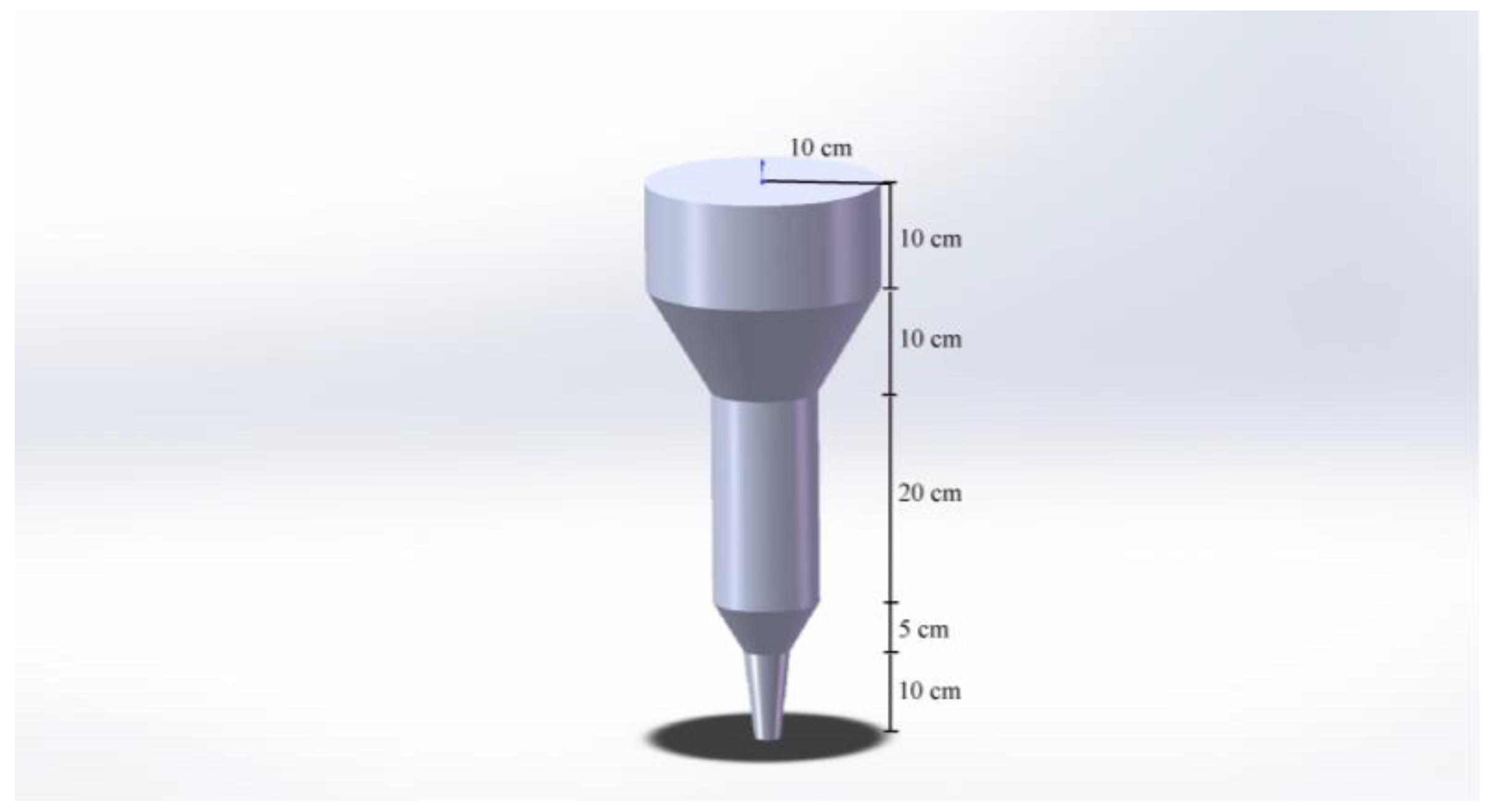
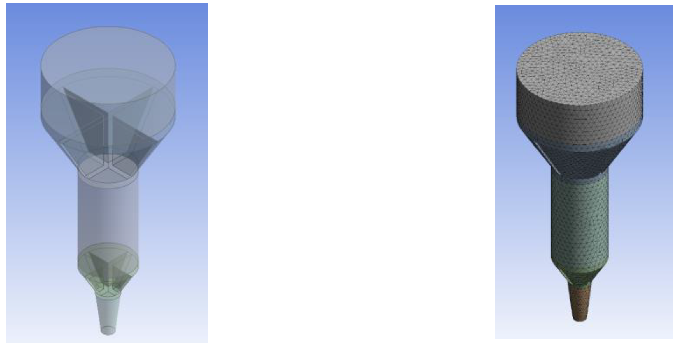
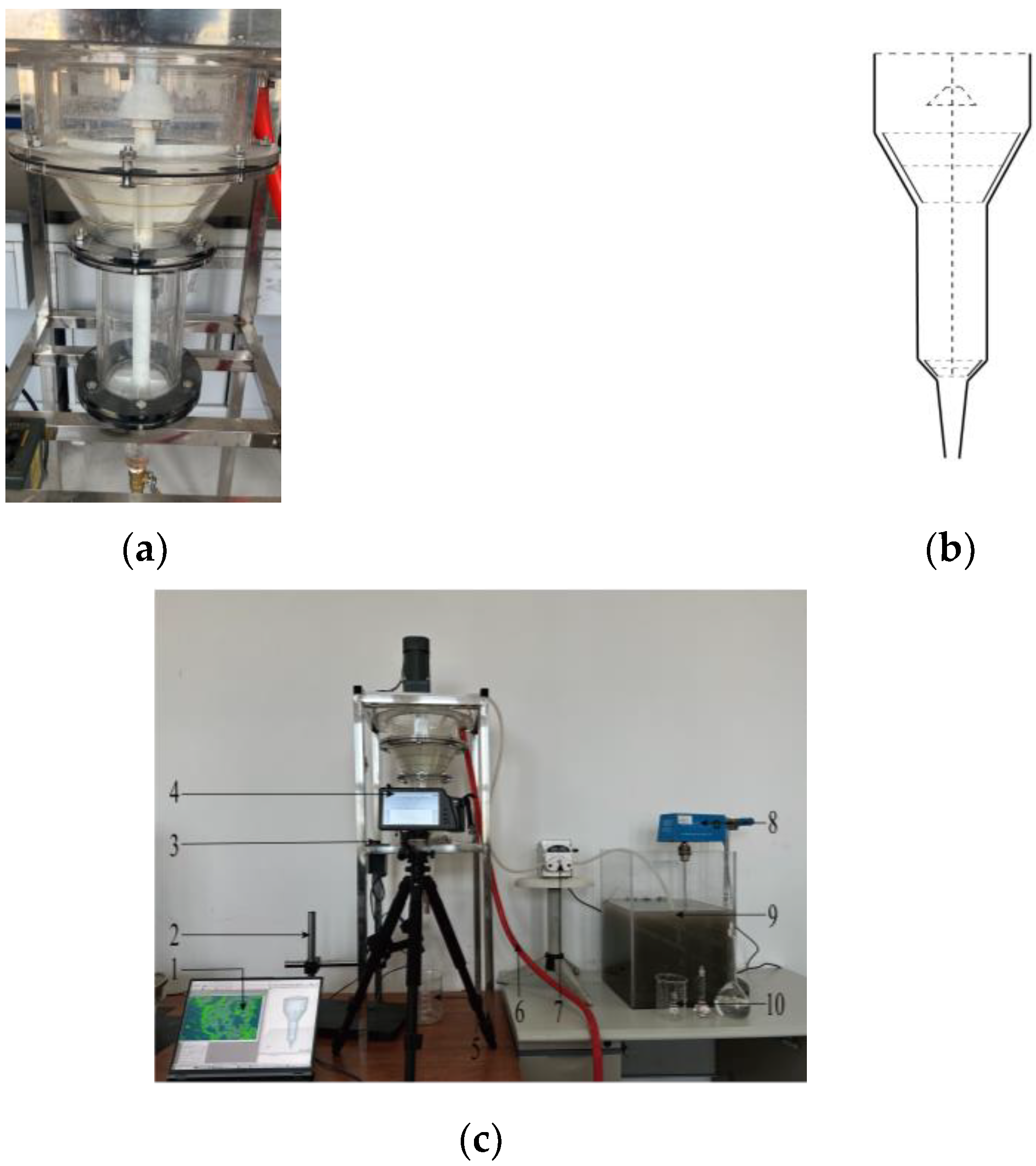
2.1. Concentrator Model

The concentrator is designed based on the principle of inclined tube settling, as shown in Figure 1. If the same concentration of mineral slurry is filled into two test tubes, one of the test tubes is placed upright (A), and the other test tube is inclined at a certain angle (B). In the case of test tube A, the settling area is only the cross-sectional area of the test tube, and the settling distance is X. On the other hand, in the case of test tube B, the settling area increases due to its inclination. Additionally, the tailing particles near the upper side of the tube also settle simultaneously due to gravity. Since the distance between the upper and lower walls is shorter, the tailings can quickly settle onto the lower division. Subsequently, the settled slurry slides down due to its weight, reducing the settling time. Therefore, test tube B requires less settling time than test tube A.

This study presents an efficient deep cone concentrator suitable for ultrafine tailings, as shown in Figure 2, which depicts the three-dimensional exterior model of the concentrator. Conventional concentrators often need more separation and excessive particle entrainment when concentrating fine tailings, leading to unsatisfactory concentration results. The novel tailings concentrator addresses these challenges by introducing an additional concentration stage. Fine particles undergo preliminary separation and concentration in the first inclined settling chamber, followed by further break and engagement in the second inclined settling chamber, thereby improving the concentration efficiency of the fine particles. Moreover, the cone angle and height of the concentrator are adjusted to accommodate the slurry characteristics of fine iron tailings, enhancing both slurry concentration and settling velocity. This reduces settling and compression time, ultimately boosting productivity [13]. Furthermore, by combining numerical simulation experiments with practical tests and calibrating the process parameters of the concentration equipment, the model’s reliability is enhanced, leveraging advancements in contemporary computational techniques.

2.2. Coupling Model Description

This study employs the dense discrete phase model (DDPM) based on the Lagrangian framework to calculate the dispersed phase volume fraction. Both DDPM and DPM introduce the concept of computing particles, but DDPM reduces computational costs by representing many actual particles as computational particles. On the other hand, the discrete phase model (DPM) does not directly consider the volume fraction of the dispersed phase and is more suitable for cases where the particle phase occupies a relatively small proportion [14]. The DDPM model, unlike the DPM model, does not explicitly consider particle collisions. However, it can be coupled with other collision models in EDEM to simulate particle–particle interactions [15].

DEM is software based on the discrete element method (DEM) and is commonly used to simulate particle behavior in a system. EDEM, a popular DEM software, does not include a fluid dynamics solver and, therefore, cannot simulate particle–fluid interactions. However, it can be coupled with a fluid dynamics solver such as ANSYS FLUENT by using the DDPM method in FLUENT. EDEM typically employs a soft sphere model to consider particle–particle interactions and their interactions with the fluid [16]. This model can transform multiple particle models into a single particle for simulation, providing more accurate results than DPM and DDPM models. Although DEM is a promising approach, it requires many calculations to search for neighboring particles, and particle collisions can be computationally expensive. Coupling the DDPM model with the DEM model allows particle behavior to be accurately simulated while reducing computational costs. This method is available in EDEM and enables more accurate particle dynamics simulations.

2.3. Mathematical Models

2.3.1. Definition and Properties of Continuous Phase and Discrete Phase

In multiphase flow, substances are typically classified into two types: continuous phase and discrete phase. The constant phase refers to substances that exist continuously in space, and macroscopic description methods can represent their hydrodynamic properties. Discrete stages refer to substances that exist discretely in an area, such as particles, and their hydrodynamic properties need to be represented by microscopic description methods. In the coupled DEM–FLUENT model, the fluid phase is the continuous phase, and the particle phase is the discrete phase.

(1) Properties and assumptions of the continuous phase include homogeneity, isotropy, and infinite divisibility. Macroscopic variables, such as density, velocity, pressure, etc., can describe the motion of the continuous phase. Interactions between particles in the ongoing phase can be neglected.

(2) Properties and assumptions of discrete phases: Discrete phases are discrete, inhomogeneous, anisotropic, and finitely divisible substances. Microscopic variables, such as position, velocity, angular velocity, etc., must describe the motion of discrete phases. Interactions between discrete phases and between discrete and continuous phases need to be considered, such as particle–particle collisions and particle–fluid interactions.

2.3.2. DDPM Method

Due to the relatively high concentration of particles, the density discrete phase model (DDPM) is employed to simulate particle flow. In the model formulation, the volume fractions of each phase are considered in the mass and momentum equations [17]. The Eulerian governing equation for the liquid phase is expressed as follows:

$$\begin{array}{l}\frac{\partial }{\partial t}\left({\alpha }_f{\rho }_f\right)+\nabla \cdot \left({\alpha }_f{\rho }_f{\overrightarrow{v}}_f\right)=0\\ \frac{\partial }{\partial t}\left({\alpha }_f{\rho }_f\right)+\nabla \cdot \left({\alpha }_f{\rho }_f{\overrightarrow{v}}_f{\overrightarrow{v}}_f\right)=-{\alpha }_f\nabla p+\nabla \cdot \left[{\alpha }_f{u}_f\left(\nabla {\overrightarrow{v}}_f+\nabla {\overrightarrow{v}}_{f^T}\right)\right]+{\alpha }_f{\rho }_f\overrightarrow{g}+{\overrightarrow{F}}_{\mathrm{exchange}}\\ \end{array}$$

(1)

where:

${\alpha }_f$—Volume fraction of continuous phase;

${\rho }_f$—Density of continuous phase;

${\overrightarrow{v}}_f$—Speed of continuous phase;

${\rho }_f$—Pressure of continuous phase;

${\overrightarrow{F}}_{\mathrm{exchange}}$—Exchange force between two terms.

To overcome the limitation of the volume fraction of the discrete phase, the model equation of particle motion [18] is as follows:

$$\begin{array}{c}{m}_P\frac{d{\overrightarrow{u}}_p}{dt}=m_P\frac{3C_d}{4}\frac{\left|{\overrightarrow{u}}_p-{\overrightarrow{u}}_f\right|}{d_P}\left({\overrightarrow{v}}_f-{\overrightarrow{u}}_f\right)+m_P/\frac{\overrightarrow{g}\left({\rho }_P-{\rho }_f\right)}{{\rho }_p}+m_P\frac{{\rho }_f}{{\rho }_p}{\overrightarrow{v}}_f\nabla {\overrightarrow{v}}_f+{\overrightarrow{F}}_{KTGF}\\ \end{array}$$

(2)

The first three terms on the right side of the equation represent the drag force, buoyancy force and air pressure gradient force, respectively. DDPM uses ${\overrightarrow{F}}_{KTGF}$ to consider the effects of inter-particle collisions and translations.

The KTGF is modeled on the basis of the solid-state force tensor:

$$\begin{array}{c}{\overrightarrow{F}}_{\mathit{KTGF}}=-m_p\frac{1}{{\rho }_p}\nabla {\stackrel{-}{\tau }}_{p0}\\ {\stackrel{-}{\tau }}_p=-p_p=+{\alpha }_p{\mu }_p\left(\nabla {\overrightarrow{u}}_p+\nabla {\overrightarrow{u}}_p^T\right)+{\alpha }_p\left({\lambda }_p-\frac{2}{3}{\mu }_p\right)\nabla \cdot {\overrightarrow{v}}_p{I}^{=}\end{array}$$

(3)

where:

$p_p$—Solid pressure;

$I^{=}$—Unit stress tensor;

${\alpha }_p$—Particle volume fraction;

${\mu }_p$ and ${\lambda }_p$—Shear viscosity and bulk viscosity due to particle momentum exchange caused by advection and collision;

${\overrightarrow{v}}_p$—Average velocity vector of the solid phase obtained from particles’ positions.

Several models can be used to quantify the drag coefficient Cd. For spherical and semi-spherical particles as well as non-spherical particles with low particle Reynolds numbers, the model proposed by Gidapsow [18] can be used, which is a combination of models from [19,20]. For fluid volume fractions higher than 0.8, it resembles the model in [20] and can be written as follows:

$$C_d=\frac{24{\alpha }_s{\rho }_f{\alpha }_f^{-2.65}}{R{e}_s}\left[1+0.15{\left({\alpha }_{f}R{e}_s\right)}^{0.687}\right]$$

(4)

where $R{e}_s$ is the particle’s Reynolds number, which is defined as follows:

$$R{e}_s=\frac{{\rho }_f{d}_s\left|{\overrightarrow{u}}_s-{\overrightarrow{v}}_f\right|}{\mu }$$

(5)

2.3.3. Turbulence Model

In this paper, the realizable k-ε turbulence model is selected. Equations (6)–(10) give the governing equations of the realizable k-ε model.

$$\begin{array}{c}\frac{\partial }{\partial t}\left(\rho k\right)+\frac{\partial }{\partial x_j}\left(\rho k{\mu }_j\right)=\frac{\partial }{\partial x_j}\left(\left(\mu +\frac{{\mu }_t}{{\sigma }_k}\right)\frac{\partial k}{\partial x_j}\right)+G_k-\rho \epsilon +S_k\\ \end{array}$$

(6)

$$\frac{\partial }{\partial t}\left(\rho \epsilon \right)+\frac{\partial }{\partial x_j}\left(\rho \epsilon {\mu }_j\right)=\frac{\partial }{\partial x_j}\left(\left(\mu +\frac{{\mu }_t}{{\sigma }_{\epsilon }}\right)\frac{\partial \epsilon }{\partial x_j}\right)+C_{1}S\rho \epsilon -C_2\rho \frac{{\epsilon }^2}{k+\sqrt{v\epsilon }}+S_{\epsilon }$$

(7)

$${\mu }_t=\rho C_{\mu }\frac{k^2}{\epsilon }$$

(8)

$$S=\sqrt{2S_{ij}{S}_{ij}}$$

(9)

$$S_{ij}=\frac{1}{2}\left(\frac{\partial u_i}{\partial x_j}+\frac{\partial u_j}{\partial x_i}\right)$$

(10)

where:

$\rho$—Fluid Density, kg·m ⁻³;

x_i, x_j—Each coordinate component;

$\partial k$, $\partial \epsilon$—The turbulent Prandtl number with turbulent kinetic energy k and dissipation rate ε;

$\mu$—Fluid Viscosity, Pa·s;

${\mu }_t$—Turbulent viscosity coefficient;

$C_1,C_2$—Model constants;

$S$—Modulus of the average strain rate tensor;

$G_k$—Turbulence generated by the mean velocity gradient;

$S_{ij}$—Shear rate tensor;

$S_k,S_{\epsilon }$—Customized source items.

2.3.4. Discrete Element JKR Contact Model

Based on the results reported in reference [20], when considering inter-particle bonding and agglomeration caused by factors such as electrostatic forces and moisture content, materials that contain moisture such as crops, ore particles, and clay require the use of the Hertz–Mindlin contact model coupled with the JKR contact model. In this study, the surface adhesion of larger stone particles and the agglomeration of fine-grained iron tailings can both be addressed using the JKR cohesion model. The bonding force between different tailings particle particles can be expressed as

$$W=r_1+r_2-r_{12}$$

(11)

The surface energies of particle 1 and particle 2 are represented in Equation (5) by r₁ and r₂, respectively. The border energy between particle 1 and particle 2 is represented by the number r₁₂.

The boundary energy between particles is zero, and the surface energy values of various particles are the same. Currently, r₁₂ = 0 and r₁ = r₂ = r. As a result, W = 2r is the equation for the cohesion between similar particle types. In Equations (12) and (13), respectively, the normal elastic contact force JKR and the normal overlap u of the particles is displayed.

$$F_{JKR}=-2({2\Pi W{E}^{*}{a}_2^3)}^{\frac{1}{2}}+\frac{4E^{*}{a}_2^3}{3R^{*}}$$

(12)

$$=\frac{a_2^2}{R^{*}}-\sqrt{\frac{2\Pi W{a}_2}{E^{*}}}$$

(13)

When W = 2r is introduced into Equations (14) and (15) and the particle types are the same, the normal elastic contact force F_JKR normal to the overlap u can be written as follows:

$$F_{JKR}=-4\sqrt{\Pi r{E}^{*}{a}_2^3}+\frac{4E^{*}{a}_2^3}{3R^{*}}$$

(14)

$$u=\frac{a_2^2}{R^{*}}-2\sqrt{\frac{\Pi W{a}_2}{E^{*}}}$$

(15)

where a₂ is the radius of the contact surface following the collision of the two particles, r is the surface energy of the contacting particles, E* is the modulus of elasticity, and R* is the equivalent contact radius.

3. Numerical Simulation Modeling

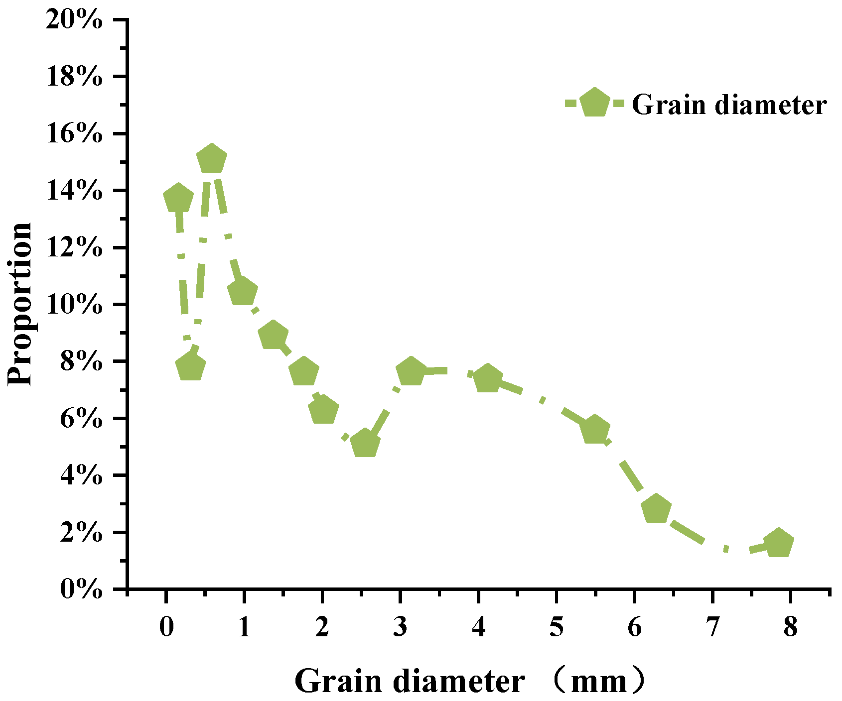
3.1. EDEM Parameter Setting

The delineated mesh shown in Figure 3 was imported into the EDEM GEOMETRY tab using the MESH module in ANSYS 17.0 software. Gravitational acceleration was set to −9.81 m/s³ on the Y axis, and the Hertz–Mindlin contact model with the JKR contact model was selected. This model is suitable for materials containing moisture, such as pharmaceutical powders, crops, ore particles, clay, and other materials where significant bonding and agglomeration occur between particles due to electrostatic forces, moisture content, etc. [21].

Therefore, the JKR cohesive force model can consider tailing accumulation and larger particles’ surface adhesion in this study. The parameters for the concentrator and solid particles are shown in

Table 1. Thickener and solid particle parameter settings.

No.	Parameters	Numerical
1	Particle Poisson’s ratio	0.3
2	Shear elasticity coefficient (pa)	2.4 × 108
3	JKR surface energy coefficient (J/m3)	0.459
4	Density (particles) (kg/m3)	2300
5	Collision recovery factor (particle)	0.2
6	Coefficient of static friction (particles)	0.395
7	Coefficient of dynamic friction (particles)	0.107
8	Collision recovery factor (wall)	0.2
9	Coefficient of static friction (wall surface)	0.5
10	Coefficient of dynamic friction (wall surface)	0.01

. The discrete element time step is set to 3 × 10⁶. The selected fine-grade iron tailing particles have relatively small particle size, and the number of material particles in the beneficiation concentrator far exceeds the current computational power level. According to reference [22], the particle size distribution after coefficient calibration is selected, as shown in Figure 4, to obtain the results of preliminary experiments. From the figure, the maximum enlarged particle size is 7.848 mm, accounting for 2.69% of the total, while the minimum particle size is 0.156 mm, accounting for 13.10%. The average particle size is 2.81 mm.

FLUENT initially set the container to be filled with water to establish a coupling connection, while EDEM adapts the concentration based on the volume of generated particles. Based on experiments, different tailing concentrations correspond to a certain number of particles. To establish a coupling connection, a certain number of particles are generated in the particle plant, and the coupling interface tool window is opened in EDEM. The start is selected to enable EDEM to listen to the coupling signal and wait for a connection to be established with FLUENT.

3.2. FLUENT Parameter Setting

The concentrator model adopts a more versatile tetrahedral mesh partitioning method for grid generation. The top is defined as the particle inlet (inlet), the bottom is the outlet (outlet), the middle cylindrical part is the wall, and the two scraper sections are defined as the fan-wall. Clicking on “Generate” generates an adapted grid. It is ensured that the size of the FLUENT fluid domain grid is at least 3 times larger than the particle grid size. Therefore, while ensuring the quality of the grid, the number of grids is minimized. In the end, the geometry is divided into 22,599 cells.

The mesh model is imported into FLUENT, and the grid quality is evaluated [23]. The fluid model is selected as transient. The difference between transient and steady-state lies in the temporal aspect. Transient calculations are based on time-dependent changes, while steady-state calculations are not affected by time and are based on the assumption that velocity and other conditions have reached a stable state. Transient models use different governing equations and require more computational resources but are closer to reality. In this study, the transient model is chosen for the coupling interface. The k-epsilon turbulence model is selected due to its high efficiency and satisfactory accuracy for engineering requirements [24]. Since the EDEM model is a continuous phase model while FLUENT is a discrete phase model, the coupling simulation requires combining these two models using a hybrid turbulence model to describe the interaction between the two phases. The SIMPLEC algorithm is selected as the solution algorithm with the “Swirl Dominated Flow” option. The time step size is set to 3 × 10⁵, 10 times the time step size of the EDEM discrete element method. The convergence criterion is set to 1 × 10⁻⁴. Boundary conditions are set for the fluid domain in FLUENT, with the concentrator inlet set as a velocity inlet and the outlet as a pressure outlet. To further improve the accuracy of numerical simulation, the motion of the scraper in the FLUENT domain is set using the Mesh Motion technique suitable for transient calculations. The rotating speed of the upper and lower scrapers is set to 10 rpm to match the particle rotation speed in the EDEM software. Finally, post-processing is performed to examine the results after achieving convergence in the actual calculations.

By taking measures to improve the reliability and accuracy of numerical simulations, such as increasing the frequency of simulation experiments to obtain the mean of 10 results, a more precise foundation has been established for further research. These efforts have enhanced the robustness and accuracy of the numerical model, ensuring that the obtained results are more reliable and can be effectively utilized for future studies.

3.3. Simulation Model Validation

For further investigation into particle motion within the vessel, numerical simulation experiments were conducted by setting the concentrator operating conditions as follows: scraper rotation speed of 10 rpm, inlet velocity of 0.26 m/s, and slurry volume concentration of 10%. The particle trajectories were post-processed using the discrete element software EDEM, and the obtained velocity profiles at different time intervals are presented in Figure 5. These results provide valuable insights into the dynamics of particle motion within the container, allowing for a comprehensive analysis of their behavior over time.

Based on the velocity profiles shown in Figure 5a, it can be observed that particles undergo free-settling motion within the container and sink upon contact with the container walls. As particles move within the container, they converge at the interface, leading to primary concentration. The constant rotational speed of the scraper ensures that particles do not linger on the walls for extended periods, maintaining fluid circulation within the container.

In Figure 5b, particles gather and flow out under pressure after reaching the bottom of the container—the height of particle accumulation at the bottom increases as the particle count at the outlet increases. As particle accumulation grows, particle motion gradually slows down, indicating the concentrator’s transition to a stable operating state.

By observing Figure 5c, the accuracy of the EDEM–FLUENT coupled model is validated. The decreasing particle velocity with increasing height of particle accumulation at the bottom suggests that the concentrator has reached a stable operating state. This preliminary validation, by the operational principles of an actual tailings concentrator, demonstrates the accuracy of the EDEM–FLUENT coupled model established in this study [25].

The EDEM software can be used to extract the motion trajectories of solid particles over time, allowing for the observation of different particle trajectories. As shown in Figure 6, after coming into contact with the wall of the container, the particles slow down during their descent. With the downward stirring effect of the upper scraper, they move towards the bottom outlet after passing the lower scraper.

In the post-processing analysis of EDEM, the particle statistics module was set at the outlet, and the corresponding particle volume data was exported. As shown in Figure 7, it can be observed that the particle volume of the concentration equipment reaches a steady state after 1 s, and the concentration of the outlet can be measured at this time.

Figure 8 and Figure 9 present volumetric concentration contour maps of particle-tracking and flow fields at different time intervals obtained from the sedimentation experiments of the concentrator. Each time interval corresponds to a diverse range of volumetric concentrations, and the scale of volumetric concentration was adjusted for a more accurate observation of its variations. The color shading on the scale represents the volumetric concentration at each location, where darker colors indicate higher concentrations, while lighter colors indicate lower concentrations. Based on the analysis of the figures, it can be observed that the volumetric concentration of the bottom layer particles reached 0.5249, equivalent to 52.490%. As the bed height increased, the volumetric concentration of the particles gradually decreased. This observed trend provides essential insights for the operation of the concentrator and serves as a reference for further research on operating conditions and improvement in concentration equipment. The clear presentation of the observed results in Figure 8 and Figure 9 ensures the accuracy and reliability of the data.

To validate the accuracy of the simulation model described above, particle sedimentation experiments were conducted. The experimental setup for the concentrator shown in Figure 10a,b illustrates the structural diagram of the concentrator, and Figure 10c presents the process flow diagram of the concentrator. The structural parameters of the concentrator are provided in

Table 2. Concentrator structural parameters.

Upper scraper diameter (cm)	22
Lower scraper diameter (cm)	10
Barrel depth (cm)	55
Tilt angle of upper scraper (°)	60
Lower scraper tilt angle (°)	45
Outlet wall inclination angle (°)	75

. The volumetric concentration of the slurry at the bottom outlet was measured under steady-state conditions, and the results were compared with the numerical simulation results.

The comparison between the experimental data and numerical simulation results is presented in Figure 11; the average volumetric concentration of the simulated results from the numerical experiments (10 trials) is 51.036%, while the average concentration obtained from the actual concentration experiments is 53.614%. The relative error between the two is only 4.800%. This comparison demonstrates the accuracy and effectiveness of the numerical model described above.

In order to validate the accuracy of the numerical simulation model, a single numerical simulation experiment was conducted under uniform operating conditions, and volumetric concentration data at different heights were obtained from both the numerical simulation and physical experiments. To facilitate comparison and analysis, the experimental data were transformed into coordinate data, with the bottom outlet as the origin, as shown in Figure 12. The concentration of the slurry at different heights along the bottom flow is presented in

Table 3. Actual experimental data.

Number	1	2	3	4	5	6
Coordinate Location	(0.0.0)	(0.10.0)	(0.20.0)	(0.30.0)	(0.40.0)	(0.50.0)
Volumetric Concentration	0.5436	0.5078	0.4389	0.3775	0.2741	0.0936

. This approach directly compares the experimental and simulated data, facilitating a comprehensive analysis of the slurry concentration curve. By adjusting the observed and simulated results on a common coordinate axis, it becomes easier to identify any similarities or differences between the two data sets. By presenting the experimental data in Table 3 and visualizing the comparative analysis in Figure 12, we ensure a rigorous examination of the accuracy of the numerical simulation model.

Based on the data in Figure 13, it can be observed that the bottom flow volumetric concentration decreases with increasing height, which is consistent with the trend observed in the laboratory experiments. This indicates that the numerical simulation results can, to some extent, reflect the actual situation. Although there is some numerical discrepancy, this is primarily attributed to the limitations of the experimental conditions, with a maximum error of 14.52% within an acceptable range. Therefore, this further validates the accuracy of the numerical simulation model.

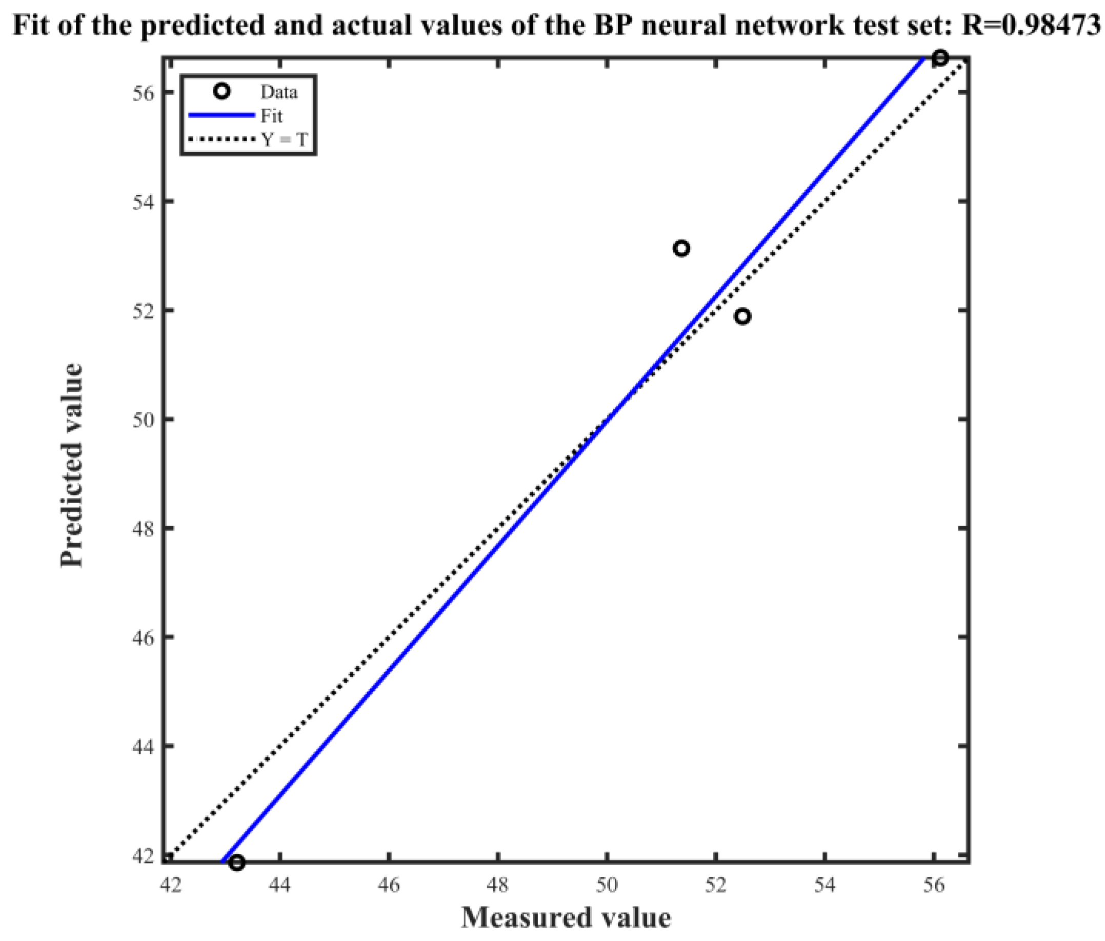
3.4. BP-NN Model Building

The reliability of the numerical simulation model can be demonstrated by verifying and comparing the numerical simulation results from different perspectives, which provides support for further study of the optimal process. To explore the optimal process more deeply, the neural network algorithm is used for analysis and study.

The BP neural network is a multi-node, feed-forward neural network with self-organizing and self-learning abilities, and is equipped with an error backpropagation algorithm. It consists of a three-layer structure: the input, hidden, and output layers. The input layer processes the variables, while the hidden layer extracts intermediate feature information by connecting the network through weights. The output layer provides the target data for prediction or analysis [26]. The network starts with the forward propagation of the input signal, followed by the backward propagation of the error. The weights and biases are adjusted iteratively to reduce error in the gradient direction, ensuring that each network parameter satisfies the minimum mistake [27].

In optimizing the simulation parameters for the thickener, selecting appropriate input layer parameters, the number of nodes in the hidden layer, and suitable model parameters for prediction are critical. The rotation speed of the double-layer scraper, inlet speed, and inlet concentration significantly impact the concentration of particles exiting the thickener and are therefore chosen as inputs to the model. However, since these factors have different units, their values vary significantly, which can affect the efficiency and accuracy of the model. To address this issue and prevent overfitting, the range of data samples was normalized to a range of [0, 1], and the normalized data were used to train the BP neural network [28,29].

To evaluate the performance of the thickener in terms of particle concentration, the outlet concentration was considered the response variable. In contrast, the rotation speed of the scraper, feed rate, and feed concentration were considered the influencing parameters. Response surface experiments were designed using the Box-Behnken module in Design Expert11, which helped identify the factors affecting the response variables and their degree of influence, as shown in

Table 4. Response surface experimental design.

Serial Number	Scraper Rotation Speed (rpm)	Feeding Speed (m/s)	Feeding Concentration (%)	Outlet Concentration (%)
1	10	0.18	7.5	56.12
2	15	0.18	5	39.66
3	15	0.1	7.5	55.35
4	10	0.18	7.5	58.33
5	5	0.18	5	43.21
6	10	0.18	7.5	56.86
7	10	0.1	5	42.45
8	10	0.26	5	45.21
9	10	0.18	7.5	54.96
10	15	0.18	10	56.33
11	10	0.18	7.5	58.41
12	5	0.26	7.5	54.84
13	15	0.26	7.5	51.37
14	5	0.18	10	50.09
15	10	0.1	10	53.63
16	5	0.1	7.5	51.37
17	10	0.26	10	52.49

. Based on the experimental results, the BP-NN model was constructed and evaluated

A total of 17 sets from the dataset in Table 4 were used as training sets, then divided into training and test sets. The training set was used to build the BP-NN model using a random function to extract 13 from the overall sample, and the remaining four were used as test sets to assess the performance and reliability of the constructed network [30]. The number of BP-NN training cycles was set to 1000, with a learning rate of 0.01, and a training error target of 0.1. The number of neural network implied nodes were evaluated and determined by analyzing the test set’s predicted mean square error and fitted value. The predicted mean square error for different implied node numbers is shown in Figure 14.

The average absolute percentage error (MAPE) of the test set samples was obtained as 2.1555% from Figure 15, which is below 3%. This indicates that the neural network has a good prediction accuracy on validation data and good generalizability.

In order to avoid overfitting, the number of implied nodes is determined to be 12, and the corresponding network training process is shown in Figure 16. As the number of iterations increases, the mean square error decreases rapidly at the beginning, and finally the change tends to level off and converges at the 3000th generation.

The comparison between the actual and predicted values of the samples when predicting the particle concentration at the outlet of the concentrator using this model is shown in Figure 17. From the figure, it can be seen that the BP-NN neural network has a positive relative error for two of the four tested samples in predicting the particle concentration at the outlet of the concentrator. This indicates that the predicted value is greater than the actual value [31]. Two samples have negative relative error, which indicates that the predicted value is less than the actual value. The experimental results show that the minimum absolute error is 0.5140, the maximum absolute error is 1.7667, the minimum relative error is 0.9158, and the maximum relative error is 3.4391. The results show that when the model is used for prediction, the predicted value of the samples is close to the actual value and the prediction error is small, and the model has a good prediction accuracy to predict the experimental data.

The fit of the test set is shown in Figure 18. The regression analysis of the proposed BP-NN network training, and the correlation coefficient between the BP-predicted and measured values is R = 0.98473. The closer the R value is to 1, the better the performance of the established model. The experimentally obtained R value is close to 1, which indicates that the established model is good and has a high prediction accuracy.

3.5. GA Advantage Search

According to the model established by BP-NN above as the fitness function of GA, GA was applied to find the maximum value of concentrator outlet concentration; set the maximum evolutionary generation of GA as 50, population size as 30, variation probability as 0.2, crossover probability as the default value of the GAOT genetic algorithm toolbox; and run to obtain the average fitness value and the best fitness curve of the population per generation, see Figure 19.

From Figure 19, it can be observed that as the number of generations increases, both the average fitness value and the best fitness value of the population show a fluctuating upward trend. After 20 iterations, the average fitness value and the best fitness value of the population tend to stabilize. When the average fitness value and the best fitness value of the population are equal, the optimal solution (predicted value) for the objective function of the genetic algorithm is obtained, with Y = 61.9992. The optimized variable values are X1 = 9.7677, X2 = 0.2037, and X3 = 6.5268, corresponding to the optimization parameters of rotation speed at 9.7677 rpm, inlet velocity at 0.2037 m/s, and inlet concentration at 6.527%. The maximum value of the outlet concentration is approximately 62.000%. Based on these parameter settings, a numerical simulation experiment was conducted, as shown in Figure 20. The average volumetric concentration of the bottom flow in the actual experiment was 60.712% (n = 10), with an error of only 2.077% compared to the predicted value. The average volumetric concentration of the outlet in the numerical simulation experiment was 59.951% (n = 10), with an error of only 3.304% compared to the predicted value. The experimental errors are within an acceptable range, indicating that the combination of BP-NN modeling and GA optimization parameters is reasonable and feasible, providing a reference for the optimization of the concentration process in the concentrator.

4. Conclusions

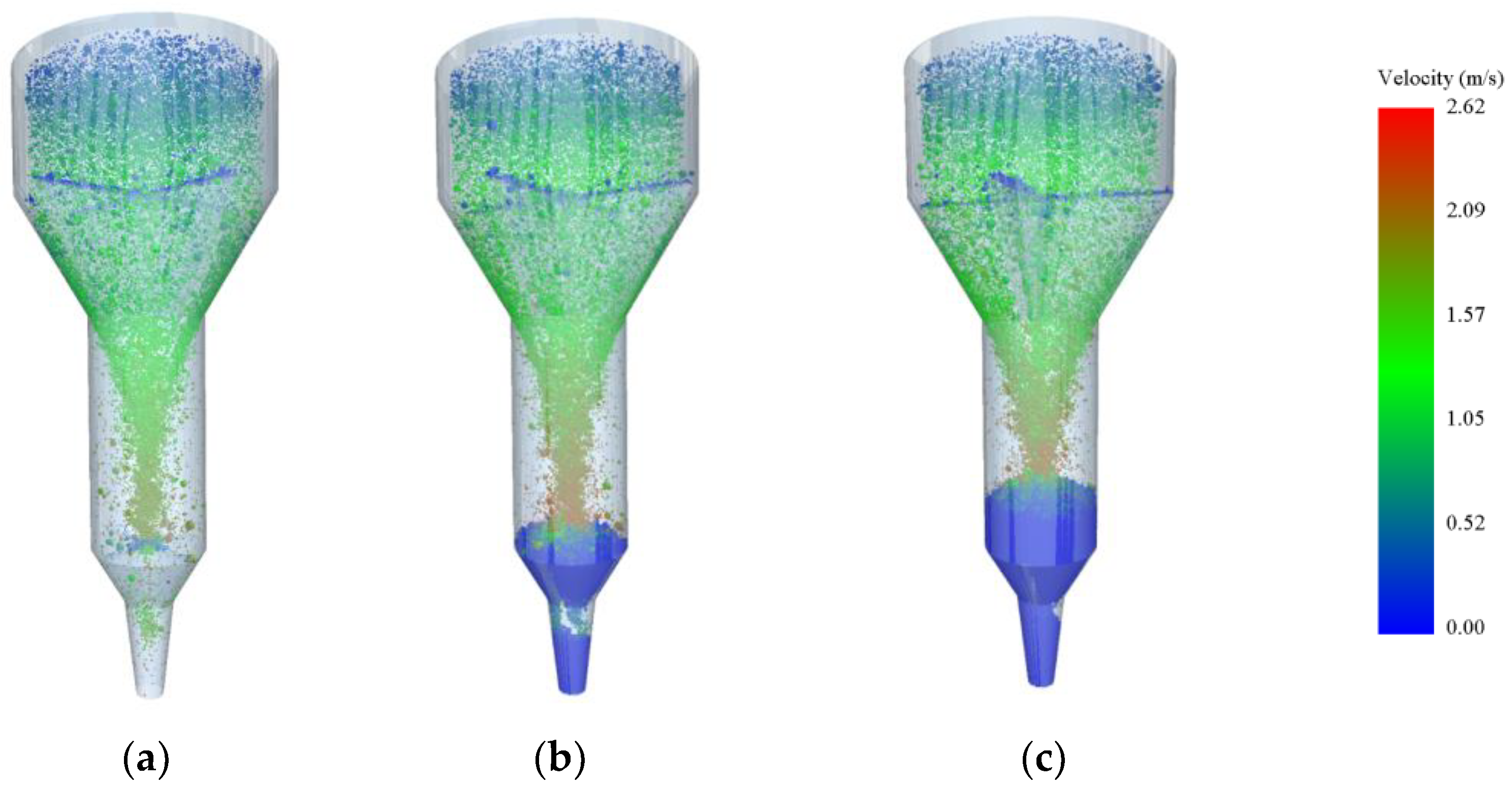
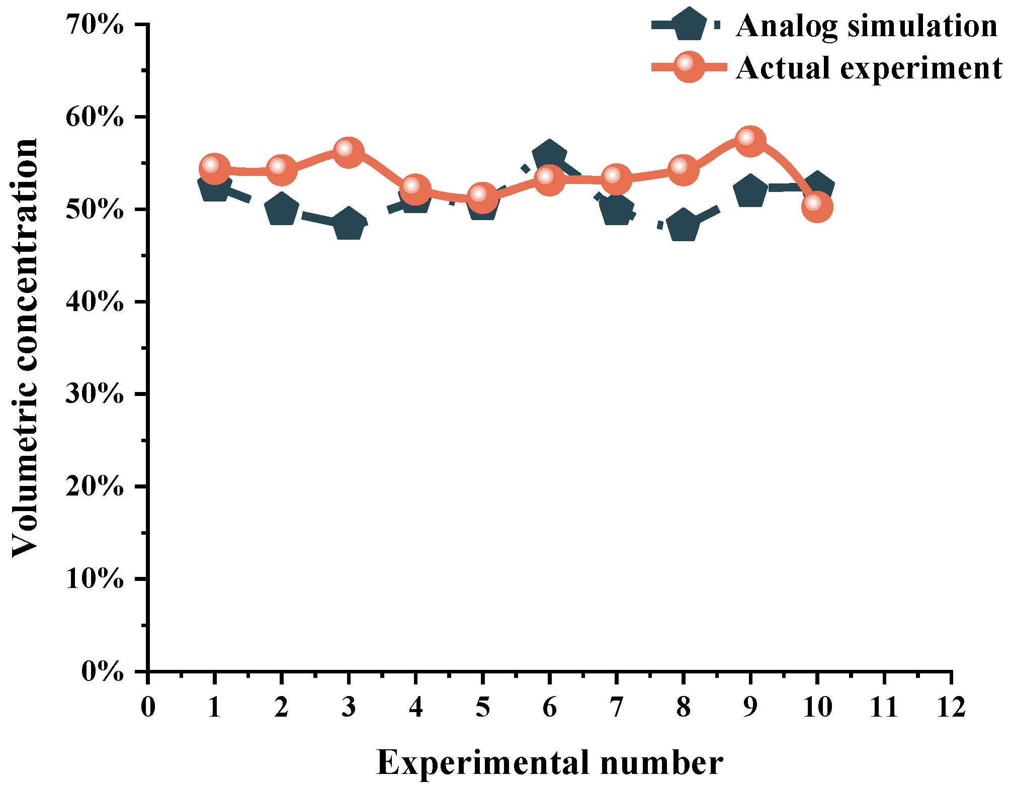
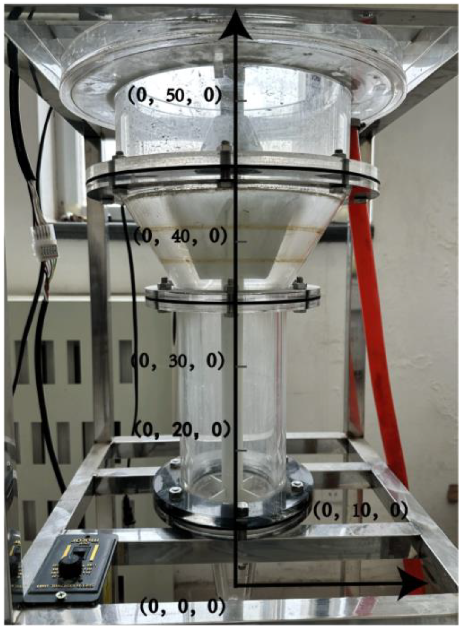
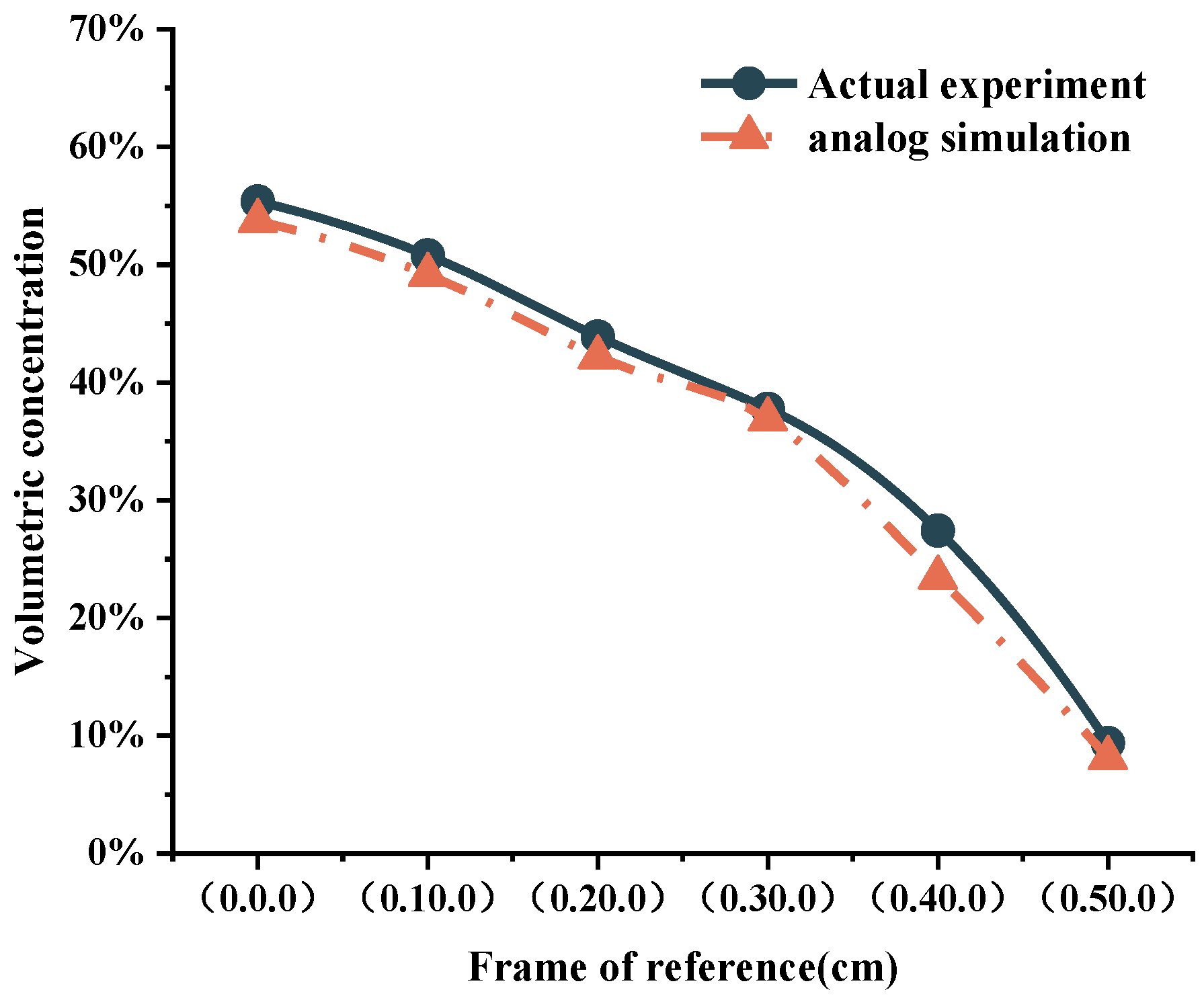
• In this study, numerical simulation using EDEM and FLUENT software was conducted to simulate the settling of concentrated particles inside the concentrator based on the theory of fluid–solid coupling. FLUENT was used to compute the fluid domain, while EDEM was employed to model the motion of particles within the system. By comparing the simulation results with actual experiments, it was found that the average volumetric concentration at the outlet in the numerical simulations (51.036%) closely matched the average volumetric concentration at the outlet in the actual concentration experiments (53.614%), with a relative error of only 4.8%. This validates the reliability of the EDEM–FLUENT model for this application. To facilitate comparison and analysis, the experimental data were transformed into coordinate axis data, using the bottom outlet as the origin. The slurry concentration at different heights was then compared. It was observed that the volumetric concentration of the bottom flow decreased with increasing height, which was consistent with the trend observed in laboratory experiments. This indicates that the numerical simulation results can, to some extent, reflect the actual situation and provide a foundation for conducting more realistic numerical simulations of the tailing concentration process in the concentrator.
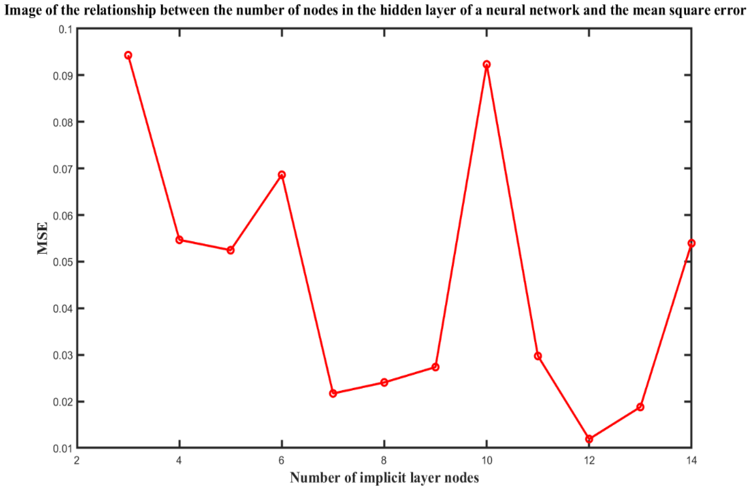
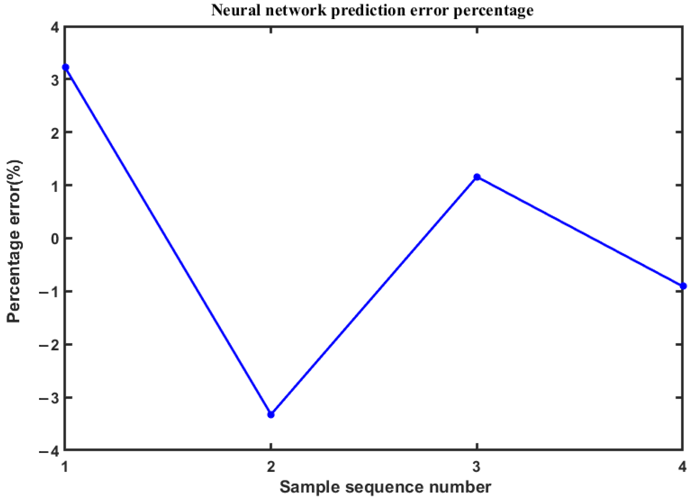
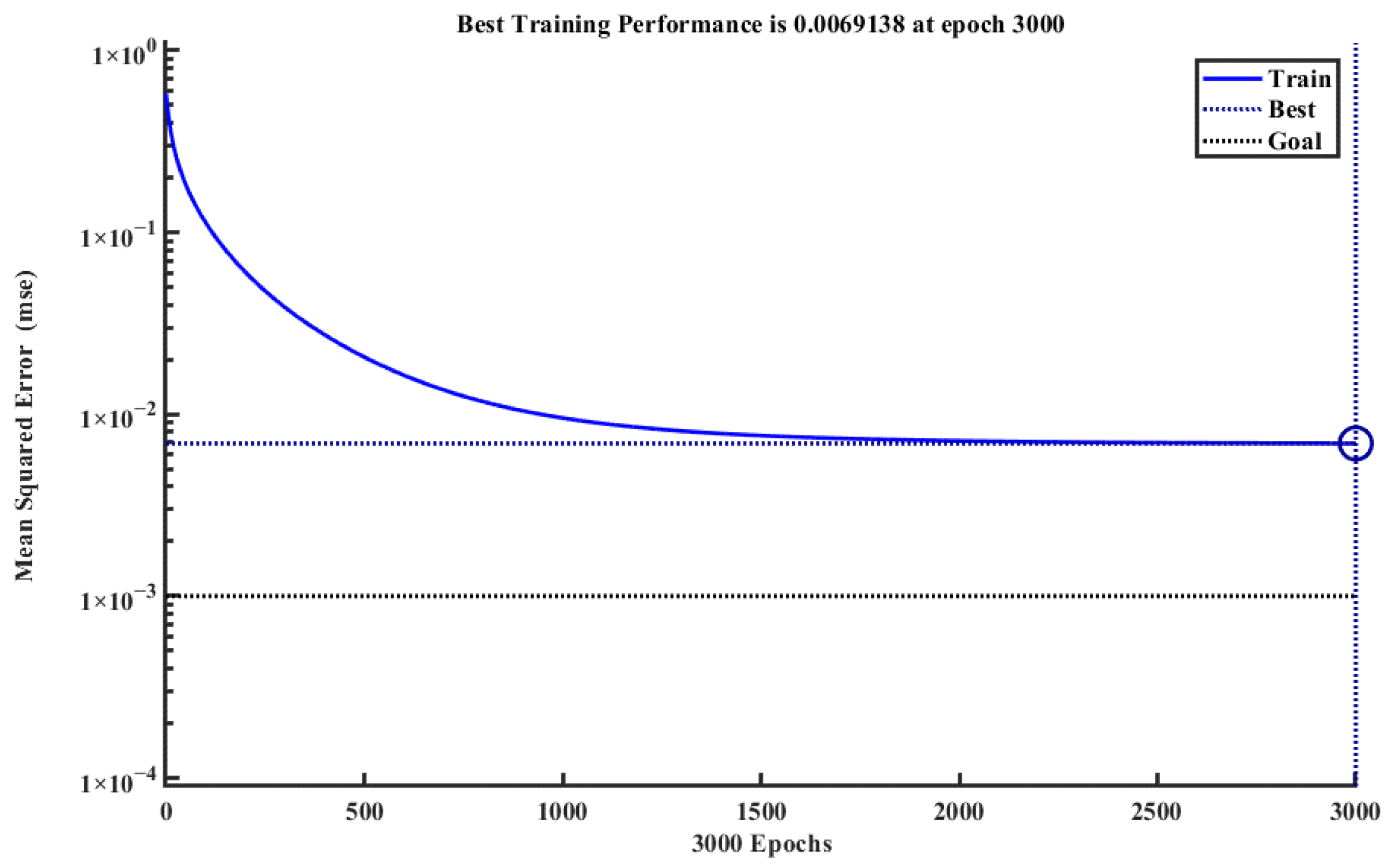
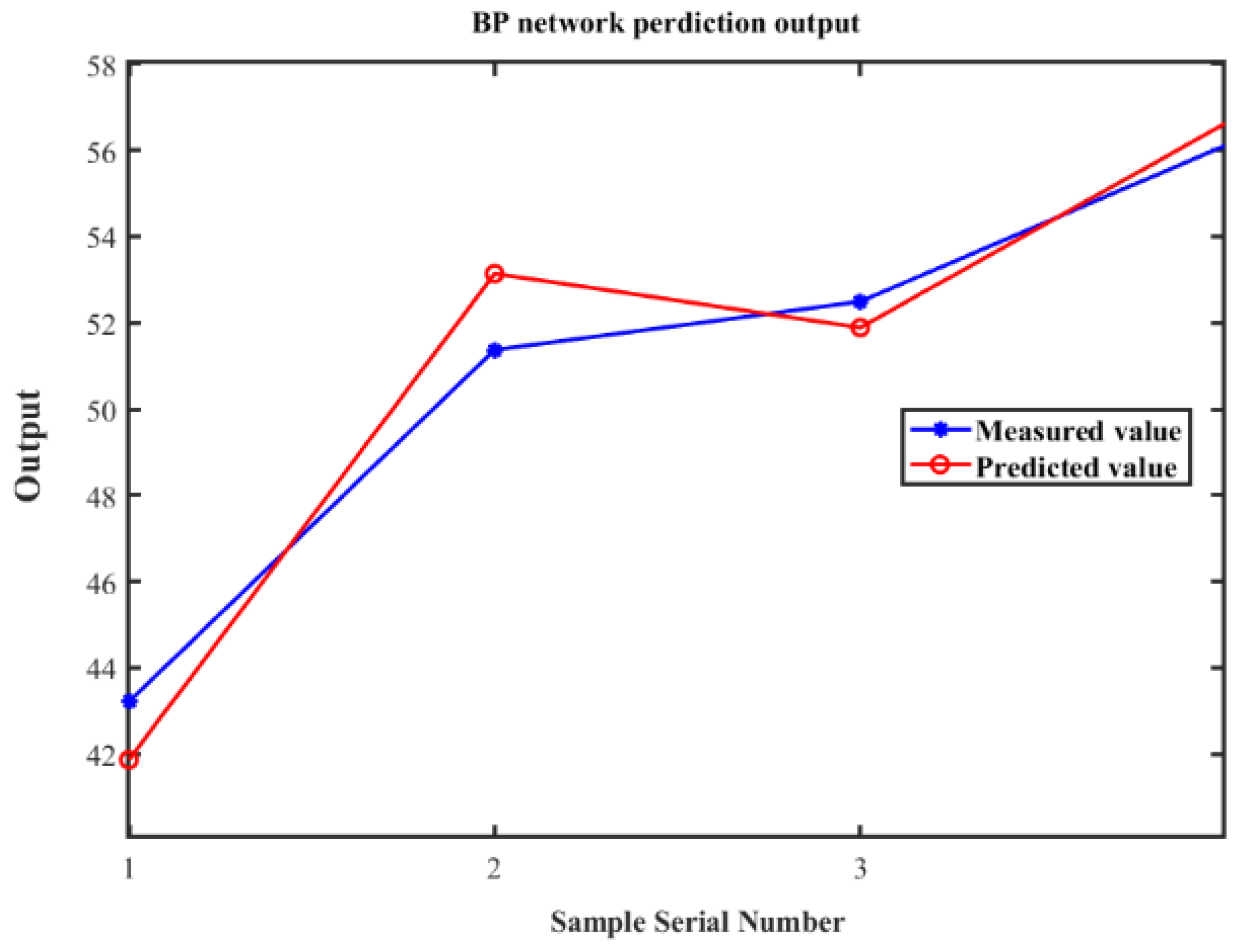
• Through response surface experiments conducted using simulation software, we trained a predictive model based on the BP-NN neural network using the results of the numerical simulation experiments. Combined with the genetic algorithm (GA), we optimized the operating parameters of the concentrator, resulting in optimized parameters of scraper rotation speed at 9.7677 rpm, feed velocity at 0.2037 m/s, and feed concentration at 6.527%. The maximum volume concentration at the bottom outlet was approximately 62.000%. We performed numerical simulation experiments based on these parameter settings, and the average volume concentration at the bottom outlet in the experiments was 60.712% (n = 10), with a deviation of only 2.077% from the predicted value. The average volume concentration at the bottom outlet in the numerical simulation experiments was 59.951% (n = 10), with a deviation of only 3.304% from the predicted value. These results demonstrate the feasibility of using BP-NN modeling combined with GA optimization for simulating parameters in the concentrator, providing a basis for optimizing the process parameters of the concentrator.

This study’s number of test cases was relatively small, and the model’s performance would be better demonstrated with a larger dataset. This is an area of future research for the authors. The use of neural networks in this paper provides a perspective for solving industrial problems, combining modern computer technology with traditional industrial practices to achieve digital transformation and provide valuable references for subsequent industrial applications.

References

1. Chen, H. Reflections on several major issues of mineral resources security and mining economic development. China Land Resour. Econ. 2020, 33, 16–20. [Google Scholar]
2. Zhang, J.; Zhu, L. Study on the characteristics of heavy metal pollution in tin mine tailing ponds. Min. Metall. 2022, 31, 122–126. [Google Scholar]
3. Ren, M.; Xie, X.; Li, B.; Hu, S.; Chen, T.; Zhu, H.; Tong, X. Research progress of comprehensive utilization of an iron tailings. Miner. Conserv. Util. 2022, 42, 155–168. [Google Scholar] [CrossRef]
4. He, J.; Wang, J.; Yu, X.; Xu, Z. Simulation and optimization analysis of centrifugal concentrator based on EDEM-FLUENT coupling. Miner. Compr. Util. 2021, 2, 174–179+140. [Google Scholar]
5. Li, H.; Li, Y.; Gao, F.; Zhao, Z.; Xu, L. CFD-DEM simulation of material motion in air-and-screencleaning device. Comput. Electron. Agric. 2012, 88, 111–119. [Google Scholar] [CrossRef]
6. Jiang, E.; Sun, Z.; Pan, Z.; Wang, L. CFD-DEM-based simulation and experiment of grain movement in harvester separation chamber. Trans. Chin. Soc. Agric. Mach. 2014, 45, 117–122. [Google Scholar]
7. Ruan, Z.; Li, C.; Shi, C. Numerical simulation of flocculation and settling behavior of whole-tailings particles in deep-cone thickener. J. Cent. South Univ. 2016, 23, 740–749. [Google Scholar] [CrossRef]
8. Majid, E.G.; Ataallah, S.G.; Alireza, A.S. Simulation of a semi-industrial pilot plant thickener using CFD approach. Int. J. Min. Sci. Technol. 2013, 23, 63–68. [Google Scholar]
9. Gheshlaghi, M.E.; Goharrizi, A.S.; Shahrivar, A.A.; Abdollahi, H. Modeling industrial thickener using computational fluid dynamics (CFD), a case study: Tailing thickener in the Sarcheshmeh copper mine. Int. J. Min. Sci. Technol. 2013, 23, 885–892. [Google Scholar] [CrossRef]
10. Zhou, S.; John, A. modelling of rectangular settling tanks. J. Hydraul. Eng. 1992, 118, 1391–1405. [Google Scholar] [CrossRef]
11. Dong, H.; Wu, K.; Kuang, Y.; Dai, M. Study of hydrate slurry separation law based on DEM-CFD hydrocyclone. J. Zhejiang Univ. 2018, 52, 1811–1820. [Google Scholar]
12. Zhao, Y.; Shen, Z.; Lu, J.; Ni, X. Simulation of leaky Rayleigh wave at air–solid cylindrical interfaces by finite element method. Ultrasonics 2006, 44, 1169–1172. [Google Scholar] [CrossRef]
13. Wu, L.; Gong, M.; Wang, J. Development of a DEM–VOF Model for the Turbulent Free-Surface Flows with Particles and Its Application to Stirred Mixing System. Ind. Eng. Chem. Res. 2018, 57, 1714–1725. [Google Scholar] [CrossRef]
14. Zhang, F.; Li, L.; Ma, X. Simulation study on the separation effect of coupled mineral particles based on EDEM-FLUENT. Miner. Compr. Util. 2022, 6, 159–166. [Google Scholar]
15. Gong, Y.; Wang, X.; Zhang, B. Amplified simulation of binary particle orientation separation process in chemical chain combustion based on DDPM model. J. Pet. (Pet. Process.) 2020, 36, 1347–1353. [Google Scholar]
16. Xu, X.; Li, F.; Shen, C.; Li, Y.; Chang, D. Optimization design and experiment of isometric screw feeding device for wheat flour. J. Agric. Mach. 2020, 51, 150–157. [Google Scholar]
17. Wang, J.; Qiu, Q.; He, X. Numerical simulation of multiphase flow mixing based on EDEM-FLUENT coupling in a stirred tank. J. Zhengzhou Univ. 2018, 39, 79–84. [Google Scholar] [CrossRef]
18. Gidaspow, D. Multiphase Flow and Fluidization: Continuum and Kinetic Theory Descriptions; Academic Press: New York, NY, USA, 1994. [Google Scholar]
19. Wen, C.Y.; Yu, Y.H. Mechanics of fluidization. Chem. Eng. Prog. Symp. 1966, 62, 100–113. [Google Scholar]
20. Ergun, S. Fluid flow through packed columns. Chem. Eng. Prog. 1952, 48, 89–94. [Google Scholar]
21. Li, R.; Xin, F.; Han, W.; Li, S.; Zhang, G. Analysis of abrasion characteristics of spiral centrifugal pump based on DDPM. J. Lanzhou Univ. Technol. 2017, 43, 54–60. [Google Scholar] [CrossRef]
22. Zhang, J.; Chang, Z.; Niu, F.; Chen, Y.; Wu, J.; Zhang, H. Simulation and Validation of Discrete Element Parameter Calibration for Fine-Grained Iron Tailings. Minerals 2022, 13, 58. [Google Scholar] [CrossRef]
23. Zhang, Y.; Wang, X. Study of flow characteristics of flocculent particle clusters in pouring pipes based on CFD-DPM model. Chem. Mach. 2023, 50, 59–66. [Google Scholar] [CrossRef]
24. Kishida, N.; Nakamura, H.; Takimoto, H.; Ohsaki, S.; Watano, S. Coarse-grained discrete element simulation of particle flow and mixing in a vertical high-shear mixer. Powder Technol. 2021, 390, 1–10. [Google Scholar] [CrossRef]
25. Wang, X.T.; Cui, B.Y.; Wei, D.C.; Song, Z.G. Simulation of internal flow field characteristics of deep cone type thickener. J. Northeast. Univ. 2020, 41, 418–423. [Google Scholar]
26. Jeldres, R.I.; Fawell, P.D.; Florio, B.J. Population balance modelling to describe the particle aggregation process: A review. Powder Technol. 2018, 326, 190–207. [Google Scholar] [CrossRef]
27. He, Y.; Guo, F.H. Micromechanical analysis on the compaction of tetrahedral particles. Chem. Eng. Res. Des. 2018, 136, 610–619. [Google Scholar] [CrossRef]
28. Kshirsagar, P.; Akojwar, S. Optimization of BPNN parameters using PSO for EEG signals. In Proceedings of the International Conference on Communication and Signal Processing 2016 (ICCASP 2016), Lonere, India, 26–27 December 2016; Volume 12, pp. 384–393. [Google Scholar]
29. Jia, H.; Chen, Y.; Zhao, J.; Guo, M.; Huang, D.; Zhuang, J. Design and key parameter optimization of an agitated soybean seed metering device with horizontal seed filling. Int. J. Agric. Biol. Eng. 2018, 11, 76–87. [Google Scholar] [CrossRef] [Green Version]
30. Zhang, L.; Wang, F.; Sun, T.; Xu, B. A constrained optimization method based on BP neural network. Neural Comput. Appl. 2018, 29, 413–421. [Google Scholar] [CrossRef]
31. Zhong, X.M.; Chen, M.Z.; Zhuang, J.; Chen, Y.; Liu, J.J.; Yang, Z.M. BP neural network combined with genetic algorithm to optimize the process conditions of rosehips and dragon fruit solid beverage. Food Ferment. Ind. 2019, 45, 173–179. [Google Scholar] [CrossRef]
Figure 1. Comparison of settling effect between straight pipe and inclined pipe. (A) Vertical settlement display (B) Inclined settlement display.
Minerals 13 00840 g001
Figure 2. Three-dimensional shell model of concentrator.
Minerals 13 00840 g002
Figure 3. Concentrator 3D prototype with mesh.
Minerals 13 00840 g003
Figure 4. Particle size distribution.
Minerals 13 00840 g004
Figure 5. Particle motion trajectory: (a) t = 0.3 s; (b) t = 0.6 s; (c) t = 1.0 s.
Minerals 13 00840 g005
Figure 6. Trajectory of single particle movement.
Minerals 13 00840 g006
Figure 7. Bottom particle volume change diagram.
Minerals 13 00840 g007
Figure 8. Numerical simulation of particle tracking concentration clouds at different moments: (a) t = 0.4 s; (b) t = 0.6 s; (c) t = 1.0 s.
Minerals 13 00840 g008
Figure 9. Flow field concentration clouds at different moments: (a) t = 0.4 s; (b) t = 0.6 s; (c) t = 1.0 s.
Minerals 13 00840 g009
Figure 10. Actual concentration experimental setup: (a) Experimental model of actual concentrator; (b) concentrator structure diagram; (c) concentration equipment flow structure diagram. 1—Numerical simulation test system. 2—CCD camera. 3—Scraper governor. 4—High-speed camera. 5—Sample beaker. 6—Overfall. 7—Peristaltic pump. 8—Stirrer. 9—Slurry-mixing tank. 10—Flocculant.
Minerals 13 00840 g010
Figure 11. Numerical simulation experiments and actual experimental results record.
Minerals 13 00840 g011
Figure 12. Concentrator axis display.
Minerals 13 00840 g012
Figure 13. Actual experiment and analog experimental data.
Minerals 13 00840 g013
Figure 14. Prediction mean square error of different implied nodes of BP-NN.
Minerals 13 00840 g014
Figure 15. Relative error of BP-NN sample set.
Minerals 13 00840 g015
Figure 16. BP-NN training error curve.
Minerals 13 00840 g016
Figure 17. Relative error of BP-NN test results.
Minerals 13 00840 g017
Figure 18. The BP-NN test set fit.
Minerals 13 00840 g018
Figure 19. GA adaptation curve.
Minerals 13 00840 g019
Figure 20. Comparison of experimental results.
Minerals 13 00840 g020