Article

Novel Concept of Energy in Bipolar Single-Valued Neutrosophic Graphs with Applications

by
Siti Nurul Fitriah Mohamad
1,2,*,
Roslan Hasni
2,
Florentin Smarandache
3 and
Binyamin Yusoff
2
1
Faculty of Computer and Mathematical Sciences, Universiti Teknologi MARA (UiTM) Kelantan, Machang 18500, Kelantan, Malaysia
2
Faculty of Ocean Engineering Technology and Informatics, Universiti Malaysia Terengganu (UMT), Kuala Nerus 21030, Terengganu, Malaysia
3
Mathematics & Science Department, University of New Mexico, 705 Gurley Ave, Gallup, NM 87301, USA
*
Author to whom correspondence should be addressed.
Axioms 2021, 10(3), 172; https://doi.org/10.3390/axioms10030172
Submission received: 6 April 2021 / Revised: 12 July 2021 / Accepted: 14 July 2021 / Published: 29 July 2021

Abstract

:
The energy of a graph is defined as the sum of the absolute values of its eigenvalues. Recently, there has been a lot of interest in graph energy research. Previous literature has suggested integrating energy, Laplacian energy, and signless Laplacian energy with single-valued neutrosophic graphs (SVNGs). This integration is used to solve problems that are characterized by indeterminate and inconsistent information. However, when the information is endowed with both positive and negative uncertainty, then bipolar single-valued neutrosophic sets (BSVNs) constitute an appropriate knowledge representation of this framework. A BSVNs is a generalized bipolar fuzzy structure that deals with positive and negative uncertainty in real-life problems with a larger domain. In contrast to the previous study, which directly used truth and indeterminate and false membership, this paper proposes integrating energy, Laplacian energy, and signless Laplacian energy with BSVNs to graph structure considering the positive and negative membership degree to greatly improve decisions in certain problems. Moreover, this paper intends to elaborate on characteristics of eigenvalues, upper and lower bound of energy, Laplacian energy, and signless Laplacian energy. We introduced the concept of a bipolar single-valued neutrosophic graph (BSVNG) for an energy graph and discussed its relevant ideas with the help of examples. Furthermore, the significance of using bipolar concepts over non-bipolar concepts is compared numerically. Finally, the application of energy, Laplacian energy, and signless Laplacian energy in BSVNG are demonstrated in selecting renewable energy sources, while optimal selection is suggested to illustrate the proposed method. This indicates the usefulness and practicality of this proposed approach in real life.

1. Introduction

The graph spectrum is applicable in statistical physics and mathematical combinatorial optimization problems. Pattern recognition, modelling virus spread in computer networks, and safeguarding personal data in databases all benefit from the spectrum of a graph. The concept of graph energy is related to a graph’s spectrum. This concept was originally introduced by Gutman [1] in 1978. It is defined as the sum of the absolute values of the eigen values of the graph’s adjacency matrix. By linking the edge of a graph to the electron energy of a type of molecule, the energy of a graph is employed in quantum theory and many other applications in the context of energy. Later, Gutman and Zhou [2] defined the Laplacian energy of a graph as the sum of the absolute values of the differences of average vertex degree of G to the Laplacian eigenvalues of G. Details on the properties of graph energy and Laplacian energy can be found in [3,4,5,6,7,8,9,10,11].
Zadeh first introduced the fuzzy set theory in 1965 [12]. After the initiation of fuzzy sets, the concept of fuzzy graphs was developed by Kaufmann [13] and Rosenfeld [14] to deal with the fuzzy environment in graphs. Zhang [15] developed the concept of a bipolar fuzzy set where a positive membership function and a negative membership function are generalized from the traditional fuzzy set. Later, Smarandache [16] introduced the concept of the neutrosophic set, which is generalized from fuzzy set theory and intuitionistic fuzzy set.
Over the years, many researchers have studied graph energy in fuzzy and neutrosophic sets. Anjali and Mathew [17] defined the energy of a graph within the fuzzy set environment. In 2014, Sharbaf and Fayazi [18] introduced the concept of Laplacian energy of fuzzy graphs and some results on Laplacian energy bounds extended to fuzzy graphs. In the same year, Praba et al. [19] discussed the energy in the intuitionistic fuzzy graph. Laplacian energy in an intuitionistic fuzzy graph was defined by Basha and Kartheek [20]. Later, Akram and Naz [21] defined the energy and Laplacian energy of Pythagorean fuzzy graphs (PFGs) and Pythagorean fuzzy digraphs (PFDGs). Moreover, the study also derived the lower and upper bounds for the energy and Laplacian energy of PFGs. Later, Murugesan and Venkatesh [22] defined energy and Laplacian energy of a bipolar fuzzy graph. Furthermore, Naz et al. [23] introduced the concept of energy of bipolar fuzzy graph (BFG) and bipolar fuzzy digraph (BFDG). The study derived the maximal energy of BFGs and investigated their properties. In 2020, Ramesh and Basha [24] defined the signless Laplacian energy of an intuitionistic fuzzy graph by implementing the cosine similarity measure in solving decision-making problems. The same author [25] also computed signless Laplacian energy of an intuitionistic fuzzy graph with TOPSIS method using MATLAB software and applied it in group decision-making problems.
Recently, Broumi et al. [26] proposed an interval-valued neutrosophic graph using MATLAB to compute energy and spectrum analysis. Later, Mohsin et al. [27] extended the energy of a fuzzy graph, intuitionistic fuzzy graph, and single-valued neutrosophic graph concepts to a complex neutrosophic graph. Naz et al. [28] introduced the concept of energy, Laplacian energy, and signless Laplacian energy in single-valued neutrosophic graphs and constructed a relation between them. In 2020, Mullai et al. [29] introduced dominating energy of a neutrosophic graph, dominating neutrosophic adjacency matrix, eigen values for the dominating energy of neutrosophic graphs, and complement of neutrosophic graphs. Table 1 summarizes some significant influences towards energy graph, Laplacian energy graph and signless Laplacian energy graph. Previous literature suggested integrating of energy, Laplacian energy, and signless Laplacian energy with single-valued neutrosophic graphs (SVNGs). This integration is used to solve problems that are characterized by indeterminate and inconsistent information. However, when the information is endowed with both positive and negative uncertainty, then BSVNs constitute an appropriate knowledge representation of this framework. Moreover, there has been no discussion concerning energy graphs in BSVNs.
Bipolarity refers to the tendency of the human mind to analyze and take responsibility based on positive and negative outcomes. The positive analysis is all about reasonable, permitted, appropriate, or considered acceptable, while impossible, rejected or forbidden represents negative analyses. Furthermore, positive thoughts correspond to the preferences as they interpret which objects are preferable to others without rejecting those that do not meet the preferences. Still, negative thoughts correspond to the constraints as they interpret which values or objects must be declined. Based on these consequences, Deli et al. [30] proposed bipolar fuzzy sets and neutrosophic sets to bipolar neutrosophic sets in which positive membership degree, negative membership degree, and operations were studied. Bipolar fuzzy sets have a great value in dealing with uncertainty in real-life problems and useful in dealing with the positive and the negative membership values. Thus, in this paper, we combined BSVNs with an energy graph and applied them to selecting renewable energy sources. In particular, this paper aims to introduce the concepts of energy, Laplacian energy, and signless Laplacian energy in BSVNG, to investigate the properties on characteristics of eigenvalues, upper and lower bound of energy, Laplacian energy and signless Laplacian energy and to present the relationship among them.
The outline of this study is organized as follows: Section 2 gives the basic concepts related to neutrosophic and bipolar sets. Section 3 defines the concepts of energy in BSVNG while the concept of Laplacian energy in BSVNG is discussed in Section 4. On the other hand, Section 5 presents the concepts of signless Laplacian energy in BSVNG and the relation between energy, Laplacian energy, and signless Laplacian energy presented in Section 6. Moreover, to implement our proposed study, we discuss the application of the energy of BSVNG in the selection of renewable energy sources in Section 7, while Section 8 provides comparative results. Finally, this study is concluded by mentioning future potential research work in Section 9.

2. Preliminaries

In this section, some concepts related to neutrosophic set and bipolar neutrosophic set are presented. For further details, the readers are referred to [31,32,33,34,35,36,37,38,39,40].
Definition 1.
[16] Let X be a universal set. The neutrosophic set (NS) A in X categorized by membership functions T A ( x ) , I A ( x ) and F A ( x ) denote the true, indeterminate and false contained in real standard and the non-standard subset of ] 0 , 1 + [ , respectively, such that:
A = { x , T A ( x ) , I A ( x ) , F A ( x ) | x X } .
There is no restriction on the sum of T A ( x ) , I A ( x ) and F A ( x ) :
0 s u p T A ( x ) + s u p I A ( x ) + s u p F A ( x ) 3 + .
Definition 2.
[30] A bipolar neutrosophic set (BNS) A in X is defined as an object of the form:
A = { x , ( T A + ( x ) , I A + ( x ) , F A + ( x ) , T A ( x ) , I A ( x ) , F A ( x ) ) | x X }
where T A + ( x ) , I A + ( x ) , F A + ( x ) : A [ 0 , 1 ] and T A ( x ) , I A ( x ) , F A ( x ) : A [ 1 , 0 ] . The positive membership degrees T A + , I A + and F A + denote the truth membership, indeterminate membership and false membership. On the other hand, negative membership degrees T A , I A and F A denote the truth membership, indeterminate membership and false membership of an element x X to some implicit counter-property corresponding to a bipolar neutrosophic set A.
Definition 3.
[30] Let  A 1 = T 1 + , I 1 + , F 1 + , T 1 , I 1 , F 1  and  A 2 = T 2 + , I 2 + , F 2 + , T 2 , I 2 , F 2  be two bipolar neutrosophic numbers, then
  • λ A 1 = 1 ( 1 T 1 + ) λ , ( I 1 + ) λ , ( F 1 + ) λ , ( T 1 ) λ , ( I 1 ) λ , ( 1 ( 1 ( F 1 ) ) ) λ ;
  • A 1 λ = ( T 1 + ) λ , 1 ( 1 I 1 + ) λ , 1 ( 1 F 1 + ) λ , ( 1 ( 1 ( T 1 ) ) ) λ , ( I 1 ) λ , ( F 1 ) λ ;
  • A 1 + A 2 = T 1 + + T 2 + T 1 + T 2 + , I 1 + I 2 + , F 1 + F 2 + , T 1 T 2 , ( I 1 I 2 I 1 I 2 ) , ( F 1 F 2 F 1 F 2 ) ;
  • A 1 A 2 = T 1 + T 2 + , I 1 + + I 2 + I 1 + I 2 + , F 1 + + F 2 + F 1 + F 2 + , ( T 1 T 2 T 1 T 2 ) , I 1 I 2 , F 1 F 2 ;
where  λ > 0 .
Definition 4.
[30] Let A 1 = T 1 + , I 1 + , F 1 + , T 1 , I 1 , F 1 be a bipolar neutrosophic number. Then, the score function s ( A 1 ) , accuracy function a ( A 1 ) and certainty function c ( A 1 ) are defined as follows:
  • s ( A 1 ) = ( T 1 + + 1 I 1 + + 1 F 1 + + 1 + T 1 I 1 F 1 ) / 6 ;
  • a ( A 1 ) = T 1 + F 1 + + T 1 I 1 ;
  • c ( A 1 ) = T 1 + F 1 + .

3. Energy of Bipolar Single-Valued Neutrosophic Graphs

In this section, we define and investigate the energy of a graph within the frameworks of BSVNG theory and discuss its properties.
Definition 5.
The adjacency matrix A ( G ¯ )  of a BSVNG G ¯ = ( α , β )  is defined as a square matrix A ( G ¯ ) = [ a p q ] , a p q = T β + ( v p v q ) , I β + ( v p v q ) , F β + ( v p v q ) , T β ( v p v q ) , I β ( v p v q ) , F β ( v p v q )  where T β + ( v p v q ) , I β + ( v p v q ) , F β + ( v p v q ) , T β ( v p v q ) , I β ( v p v q ) and F β ( v p v q )  represent the strength of a positive relationship, the strength of a positive undecided relationship, the strength of a positive non-relationship, the strength of a negative relationship, the strength of a negative undecided relationship and the strength of a negative non-relationship between u p  and u q , respectively.
The adjacency matrix of a BSVNG can be expressed as six matrices. The first matrix contains the elements as positive truth-membership values; the second matrix contains the elements as positive indeterminacy-membership values; the third matrix contains the elements as positive falsity-membership values; the fourth matrix contains the elements as negative truth-membership values; the fifth matrix contains the elements as negative indeterminacy-membership values; and the sixth matrix contains the elements as negative falsity-membership values, i.e.,
A ( G ¯ ) = A ( T β + ( v p v q ) ) , A ( I β + ( v p v q ) ) , A ( F β + ( v p v q ) ) , A ( T β ( v p v q ) ) , A ( I β ( v p v q ) ) , A ( F β ( v p v q ) ) .
Definition 6.
The spectrum of adjacency matrix of a BSVNG A ( G ¯ )  is defined as R , S , T , U , V , W ,where R , S , T , U , V  and W  are the sets of eigenvalues of:
A ( T β + ( v p v q ) ) , A ( I β + ( v p v q ) ) , A ( F β + ( v p v q ) ) , A ( T β ( v p v q ) ) , A ( I β ( v p v q ) ) , A ( F β ( v p v q ) ) ,  respectively.
Example 1.
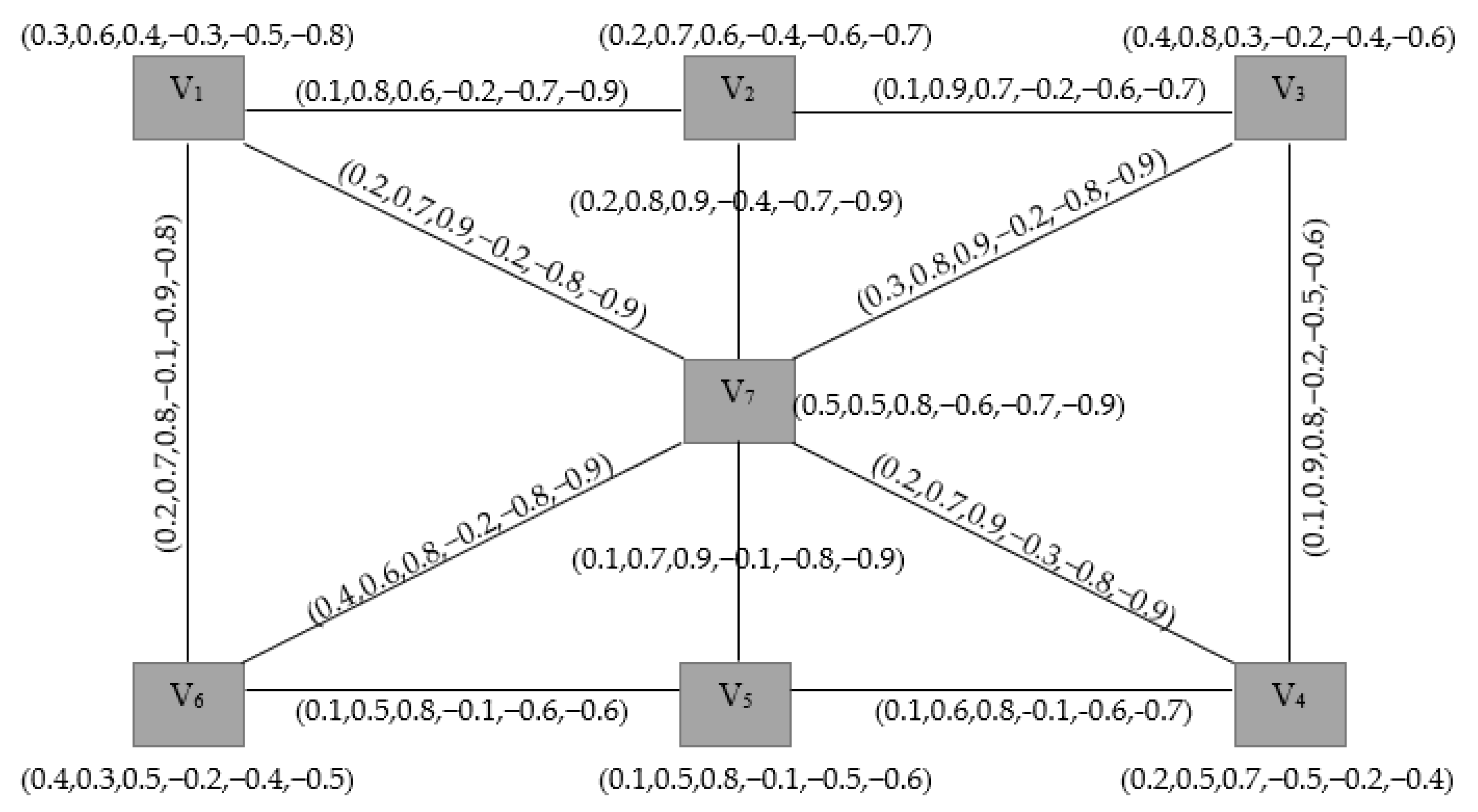
Consider a graph G ( V , E ) where V = { v 1 , v 2 , v 3 , v 4 , v 5 , v 6 , v 7 } and E = { v 1 v 2 , v 1 v 3 , v 1 v 4 , v 1 v 5 , v 1 v 6 , v 1 v 7 , v 2 v 3 , v 3 v 4 , v 4 v 5 , v 5 v 6 , v 6 v 7 } . Let G ¯ ( α , β ) be a BSVNG on V, as shown in Figure 1, defined by Table 2 and Table 3 as follows:
The adjacency matrix of a BSVNG given in Figure 1 is
( 0 , 0 , 0 , 0 , 0 , 0 0.1 , 0.8 , 0.8 , 0.1 , 0.6 , 0.9 0.2 , 0.6 , 0.9 , 0.2 , 0.4 , 0.7 0.3 , 0.7 , 0.8 , 0.1 , 0.5 , 0.8 0.4 , 0.6 , 0.7 , 0.3 , 0.6 , 0.7 0.1 , 0.5 , 0.9 , 0.1 , 0.4 , 0.7 0.3 , 0.6 , 0.9 , 0.4 , 0.4 , 0.8 0.1 , 0.8 , 0.8 , 0.1 , 0.6 , 0.9 0 , 0 , 0 , 0 , 0 , 0 0.1 , 0.9 , 0.5 , 0.1 , 0.6 , 0.9 0 , 0 , 0 , 0 , 0 , 0 0 , 0 , 0 , 0 , 0 , 0 0 , 0 , 0 , 0 , 0 , 0 0 , 0 , 0 , 0 , 0 , 0 0.2 , 0.6 , 0.9 , 0.2 , 0.4 , 0.7 0.1 , 0.9 , 0.5 , 0.1 , 0.6 , 0.9 0 , 0 , 0 , 0 , 0 , 0 0.2 , 0.8 , 0.5 , 0.1 , 0.5 , 0.6 0 , 0 , 0 , 0 , 0 , 0 0 , 0 , 0 , 0 , 0 , 0 0 , 0 , 0 , 0 , 0 , 0 0.3 , 0.7 , 0.8 , 0.1 , 0.5 , 0.8 0 , 0 , 0 , 0 , 0 , 0 0.2 , 0.8 , 0.5 , 0.1 , 0.5 , 0.6 0 , 0 , 0 , 0 , 0 , 0 0.5 , 0.8 , 0.4 , 0.1 , 0.6 , 0.7 0 , 0 , 0 , 0 , 0 , 0 0 , 0 , 0 , 0 , 0 , 0 0.4 , 0.6 , 0.7 , 0.3 , 0.6 , 0.7 0 , 0 , 0 , 0 , 0 , 0 0 , 0 , 0 , 0 , 0 , 0 0.5 , 0.8 , 0.4 , 0.1 , 0.6 , 0.7 0 , 0 , 0 , 0 , 0 , 0 0.2 , 0.7 , 0.6 , 0.2 , 0.5 , 0.5 0 , 0 , 0 , 0 , 0 , 0 0.1 , 0.5 , 0.9 , 0.1 , 0.4 , 0.7 0 , 0 , 0 , 0 , 0 , 0 0 , 0 , 0 , 0 , 0 , 0 0 , 0 , 0 , 0 , 0 , 0 0.2 , 0.7 , 0.6 , 0.2 , 0.5 , 0.5 0 , 0 , 0 , 0 , 0 , 0 0.1 , 0.6 , 0.7 , 0.2 , 0.6 , 0.5 0.3 , 0.6 , 0.9 , 0.4 , 0.4 , 0.8 0 , 0 , 0 , 0 , 0 , 0 0 , 0 , 0 , 0 , 0 , 0 0 , 0 , 0 , 0 , 0 , 0 0 , 0 , 0 , 0 , 0 , 0 0.1 , 0.6 , 0.7 , 0.2 , 0.6 , 0.5 0 , 0 , 0 , 0 , 0 , 0 )
The spectrum of a BSVNG G ¯ , given in Figure 1, is as follows:
S p e c ( T β + ( v p v q ) ) = { 0.6163 , 0.4338 , 0.1208 , 0.0406 , 0.1252 , 0.1495 , 0.9369 } . S p e c ( I β + ( v p v q ) ) = { 1.4555 , 1.1839 , 0.7335 , 0.3342 , 0.4205 , 0.9179 , 2.3687 } . S p e c ( F β + ( v p v q ) ) = { 1.6620 , 0.9839 , 0.6946 , 0.1998 , 0.2355 , 0.7439 , 2.5609 } . S p e c ( T β ( v p v q ) ) = { 0.7265 , 0.1609 , 0.0509 , 0.0476 , 0.1242 , 0.1464 , 0.6202 } . S p e c ( I β ( v p v q ) ) = { 1.7702 , 0.7044 , 0.3299 , 0.2795 , 0.5615 , 0.9685 , 0.9950 } . S p e c ( F β ( v p v q ) ) = { 2.5122 , 0.8107 , 0.4128 , 0.3321 , 0.7283 , 1.1356 , 1.5398 } .
Therefore,
S p e c ( G ¯ ) = { 0.6163 , 1.4555 , 1.6620 , 0.7265 , 1.7702 , 2.5122 , 0.4338 , 1.1839 , 0.9839 , 0.1609 , 0.7044 , 0.8107 , 0.1208 , 0.7335 , 0.6946 , 0.0509 , 0.3299 , 0.4128 , 0.0406 , 0.3342 , 0.1998 , 0.0476 , 0.2795 , 0.3321 , 0.1252 , 0.4205 , 0.2355 , 0.1242 , 0.5615 , 0.7283 , 0.1495 , 0.9179 , 0.7439 , 0.1464 , 0.9685 , 1.1356 , 0.9369 , 2.3687 , 2.5609 , 0.6202 , 0.9950 , 1.5398 } .
Definition 7.
The energy of a BSVNG G ¯ ( α , β ) is defined as
E ( G ¯ ) = E ( T β + ( v p v q ) ) , E ( I β + ( v p v q ) ) , E ( F β + ( v p v q ) ) , E ( T β ( v p v q ) ) , E ( I β ( v p v q ) ) , E ( F β ( v p v q ) ) = p = 1 λ p R n | λ p | , p = 1 δ p S n | δ p | , p = 1 γ p T n | γ p | , p = 1 ω p U n | ω p | , p = 1 ξ p V n | ξ p | , p = 1 ψ p W n | ψ p | .
Definition 8.
Two BSVNG with the same number of vertices and the same energy are called equienergetic.
Theorem 1.
Let G ¯ ( α , β )  be a BSVNG and A ( G ¯ )  be its adjacency matrix. If λ 1 λ 2 λ n , δ 1 δ 2 δ n , γ 1 γ 2 γ n , ω 1 ω 2 ω n , ξ 1 ξ 2 ξ n and ψ 1 ψ 2 ψ n  are the eigenvalues of
A ( T β + ( v p v q ) ) , A ( I β + ( v p v q ) ) , A ( F β + ( v p v q ) ) , A ( T β ( v p v q ) ) , A ( I β ( v p v q ) ) , A ( F β ( v p v q ) ) ,
respectively.
Then,
  • p = 1 λ p R n λ p = 0 , p = 1 δ p S n δ p = 0 , p = 1 γ p T n γ p = 0 , p = 1 ω p U n ω p = 0 , p = 1 ξ p V n ξ p = 0 and p = 1 ψ p W n ψ p = 0 .
  • p = 1 λ p R n λ p 2 = 2 1 p < q n ( T β + ( v p v q ) ) 2 , p = 1 δ p R n δ p 2 = 2 1 p < q n ( I β + ( v p v q ) ) 2 , p = 1 γ p R n γ p 2 = 2 1 p < q n ( F β + ( v p v q ) ) 2 ,
    p = 1 ω p R n ω p 2 = 2 1 p < q n ( T β ( v p v q ) ) 2 , p = 1 ξ p R n ξ p 2 = 2 1 p < q n ( I β ( v p v q ) ) 2 and p = 1 ψ p R n ψ p 2 = 2 1 p < q n ( F β ( v p v q ) ) 2 .
Proof. 
  • Since A ( G ¯ ) is a symmetric matrix with zero traces, its eigenvalues are real with a sum equal to zero.
  • By trace properties of a matrix, we have
    t r ( ( A ( T β + ( v p v q ) ) ) 2 ) = p = 1 λ p R n λ p 2 ,
    where
    t r ( ( A ( T β + ( v p v q ) ) ) 2 ) = ( 0 + ( T β + ( v 1 v 2 ) ) 2 + + ( T β + ( v 1 v n ) ) 2 ) + ( ( T β + ( v 2 v 1 ) ) 2 + 0 + + ( T β + ( v 2 v n ) ) 2 ) + + ( ( T β + ( v n v 1 ) ) 2 + ( T β + ( v n v 2 ) ) 2 + + 0 ) = 2 1 p < q n n ( T β + ( v p v q ) ) 2 .
Hence, p = 1 λ p R n λ p 2 = 2 1 p < q n ( T β + ( v p v q ) ) 2 . Similarly, we can show that
p = 1 δ p R n δ p 2 = 2 1 p < q n ( I β + ( v p v q ) ) 2 , p = 1 γ p R n γ p 2 = 2 1 p < q n ( F β + ( v p v q ) ) 2 , p = 1 ω p R n ω p 2 = 2 1 p < q n ( T β ( v p v q ) ) 2 , p = 1 ξ p R n ξ p 2 = 2 1 p < q n ( I β ( v p v q ) ) 2 a n d p = 1 ψ p R n ψ p 2 = 2 1 p < q n ( F β ( v p v q ) ) 2 .
Example 2.
Consider a BSVNG G ¯ ( α , β ) on V = { v 1 , v 2 , v 3 , v 4 , v 5 , v 6 , v 7 } as shown in Figure 1. Then
E ( T β + ( v p v q ) ) = 2.4231 , E ( I β + ( v p v q ) ) = 7.4142 , E ( F β + ( v p v q ) ) = 7.0806 , E ( T β ( v p v q ) ) = 1.8767 , E ( I β ( v p v q ) ) = 5.609 , E ( F β ( v p v q ) ) = 7.4715 .
Therefore, E ( G ¯ ) = 2.4231 , 7.4142 , 7.0806 , 1.8767 , 5.6090 , 7.4715 . Also, we have
p = 1 λ p R 7 λ p = 0.6163 0.4338 0.1208 0.0406 + 0.1252 + 0.1495 + 0.9369 = 0 ,
p = 1 δ p S 7 δ p = 1.4555 1.1839 0.7335 0.3342 + 0.4205 + 0.9179 + 2.3687 = 0 , p = 1 γ p T 7 γ p = 1.6620 0.9839 0.6946 0.1998 + 0.2355 + 0.7439 + 2.5609 = 0 , p = 1 ω p U 7 ω p = 0.7265 0.1609 0.0509 + 0.0476 + 0.1242 + 0.1464 + 0.6202 = 0 , p = 1 ξ p V 7 ξ p = 1.7702 0.7044 0.3299 + 0.2795 + 0.5615 + 0.9685 + 0.9950 = 0 , p = 1 ψ p W 7 ψ p = 2.5122 0.8107 0.4128 + 0.3321 + 0.7283 + 1.1356 + 1.5398 = 0 . p = 1 λ p R 7 λ p 2 = 1.5000 = 2 ( 0.7500 ) = 2 1 p < q 7 ( T β + ( v p v q ) ) 2 , p = 1 δ p S 7 δ p 2 = 10.7999 = 2 ( 5.3999 ) = 2 1 p < q 7 ( I β + ( v p v q ) ) 2 , p = 1 γ p T 7 γ p 2 = 11.4197 = 2 ( 5.7099 ) = 2 1 p < q 7 ( F β + ( v p v q ) ) 2 , p = 1 ω p U 7 ω p 2 = 0.9800 = 2 ( 0.4900 ) = 2 1 p < q 7 ( T β ( v p v q ) ) 2 , p = 1 ξ p V 7 ξ p 2 = 6.0600 = 2 ( 3.0300 ) = 2 1 p < q 7 ( I β ( v p v q ) ) 2 , p = 1 ψ p W 7 ψ p 2 = 11.4401 = 2 ( 5.7200 ) = 2 1 p < q 7 ( F β ( v p v q ) ) 2 .
We now give upper and lower bounds of energy of a BSVNG G ¯ in terms of the number of vertices and the sum of squares of positive truth-membership, positive indeterminacy-membership, positive falsity-membership, negative truth-membership values, negative indeterminacy-membership values, and negative falsity-membership values of the edges.
Theorem 2.
Let G ¯ ( α , β ) be a BSVNG on n vertices with an adjacency matrix A ( G ¯ ) = A ( T β + ( v p v q ) ) , A ( I β + ( v p v q ) ) , A ( F β + ( v p v q ) ) , A ( T β ( v p v q ) ) , A ( I β ( v p v q ) ) , A ( F β ( v p v q ) ) .  Then
  • 2 1 p < q n ( T β + ( v p v q ) ) 2 + n ( n 1 ) | T β + | 2 n E ( T β + ( v p v q ) ) 2 n 1 p < q n ( T β + ( v p v q ) ) 2
  • 2 1 p < q n ( I β + ( v p v q ) ) 2 + n ( n 1 ) | I β + | 2 n E ( I β + ( v p v q ) ) 2 n 1 p < q n ( I β + ( v p v q ) ) 2
  • 2 1 p < q n ( F β + ( v p v q ) ) 2 + n ( n 1 ) | F β + | 2 n E ( F β + ( v p v q ) ) 2 n 1 p < q n ( F β + ( v p v q ) ) 2
  • 2 1 p < q n ( T β ( v p v q ) ) 2 + n ( n 1 ) | T β | 2 n E ( T β ( v p v q ) ) 2 n 1 p < q n ( T β ( v p v q ) ) 2
  • 2 1 p < q n ( I β ( v p v q ) ) 2 + n ( n 1 ) | I β | 2 n E ( I β ( v p v q ) ) 2 n 1 p < q n ( I β ( v p v q ) ) 2
  • 2 1 p < q n ( F β ( v p v q ) ) 2 + n ( n 1 ) | F β | 2 n E ( F β ( v p v q ) ) 2 n 1 p < q n ( F β ( v p v q ) ) 2 ,
where  | T β + | , | I β + | , | F β + | , | T β | , | I β |   and   | F β |  are the determinant of A ( T β + ( v p v q ) ) , A ( I β + ( v p v q ) ) , A ( F β + ( v p v q ) ) , A ( T β ( v p v q ) ) , A ( I β ( v p v q ) )   a n d   A ( F β ( v p v q ) ) ,  respectively.
Proof. 
i. Upper bound:
Apply Cauchy-Schwarz inequality to the vectors ( 1 , 1 , , 1 ) and ( | λ 1 | , | λ 2 | , , | λ n | ) with n entries, then
p = 1 n | λ p | n p = ` n | λ p | 2 ,
( p = 1 n λ p ) 2 = p = 1 n | λ p | 2 + 2 1 p < q n λ p λ q .
By comparing the coefficients of λ n 2 in the characteristic polynomial
p = 1 n ( λ λ p ) = | A ( G ¯ ) λ I | ,
we obtain
1 p < q n λ p λ q = 1 p < q n ( T β + ( v p v q ) ) 2 .
Substituting (3) in (2), we obtain
p = 1 n | λ p | 2 = 2 1 p < q n ( T β + ( v p v q ) ) 2 .
Meanwhile, substituting (4) in (1), we obtain
p = 1 n | λ p | n 2 1 p < q n ( T β + ( v p v q ) ) 2 = 2 n 1 p < q n ( T β + ( v p v q ) ) 2 .
Therefore,
E ( T β + ( v p v q ) ) 2 n 1 p < q n ( T β + ( v p v q ) ) 2 .
ii. Lower bound:
( E ( T β + ( v p v q ) ) ) 2 = ( p = 1 n | λ p | ) 2 = p = 1 n | λ p | 2 + 2 1 p < q n | λ p λ q | = 2 1 p < q n ( T β + ( v p v q ) ) 2 + 2 n ( n 1 ) 2 A M { | λ p λ q | } .
Since A M { | λ p λ q | } G M { | λ p λ q | } , 1 p < q n , s o
E ( T β + ( v p v q ) ) 2 1 p < q n ( T β + ( v p v q ) ) 2 + n ( n 1 ) G M { | λ p λ q | } .
Also, since
G M { | λ p λ q | } = ( 1 p < q n | λ p λ q | ) 2 n ( n 1 ) = ( p = 1 n | λ p | n 1 ) 2 n ( n 1 ) = ( p = 1 n | λ p | ) 2 n = | T β + | 2 n ,
then,
E ( T β + ( v p v q ) ) 2 1 p < q n ( T β + ( v p v q ) ) 2 + n ( n 1 ) | T β + | 2 n .
Thus,
2 1 p < q n ( T β + ( v p v q ) ) 2 + n ( n 1 ) | T β + | 2 n E ( T β + ( v p v q ) ) 2 n 1 p < q n ( T β + ( v p v q ) ) 2 .
Similarly, we can show that
2 1 p < q n ( I β + ( v p v q ) ) 2 + n ( n 1 ) | I β + | 2 n E ( I β + ( v p v q ) ) 2 n 1 p < q n ( I β + ( v p v q ) ) 2 , 2 1 p < q n ( F β + ( v p v q ) ) 2 + n ( n 1 ) | F β + | 2 n E ( F β + ( v p v q ) ) 2 n 1 p < q n ( F β + ( v p v q ) ) 2 , 2 1 p < q n ( T β ( v p v q ) ) 2 + n ( n 1 ) | T β | 2 n E ( T β ( v p v q ) ) 2 n 1 p < q n ( T β ( v p v q ) ) 2 , 2 1 p < q n ( I β ( v p v q ) ) 2 + n ( n 1 ) | I β | 2 n E ( I β ( v p v q ) ) 2 n 1 p < q n ( I β ( v p v q ) ) 2 , 2 1 p < q n ( F β ( v p v q ) ) 2 + n ( n 1 ) | F β | 2 n E ( F β ( v p v q ) ) 2 n 1 p < q n ( F β ( v p v q ) ) 2 .
Example 3.
(Illustration to Theorem 2)For the BSVNG G ¯ , given in Figure 1, E ( T β + ( v p v q ) ) = 2.4231 , lower bound = 1.8670 and upper bound = 3.2400, therefore, 1.8670 2.4231 3.2400 . E ( I β + ( v p v q ) ) = 7.4142 , lower bound = 6.5423 and upper bound = 8.6940, therefore, 6.5423 7.4142 8.6940 . E ( F β + ( v p v q ) ) = 7.0806 , lower bound = 5.7693 and upper bound = 8.9408, therefore, 5.7693 7.0806 8.9408 . E ( T β ( v p v q ) ) = 1.8767 , lower bound = 0.9899 and upper bound = 2.6192, therefore, 0.9899 1.8767 2.6192 . E ( I β ( v p v q ) ) = 5.6090 , lower bound = 2.4664 and upper bound = 6.5131, therefore, 2.4664 5.6090 6.5131 . E ( F β ( v p v q ) ) = 7.4715 , lower bound = 3.4926 and upper bound = 8.9487, therefore, 3.4926 7.4715 8.9487 .

4. Laplacian Energy of Bipolar Single-Valued Neutrosophic Graphs (BSVNG)

Definition 9.
Let G ¯ ( α , β )  be a BSVNG on n vertices. Then, the degree matrix
D ( G ¯ ) = D ( T β + ( v p v q ) ) , D ( I β + ( v p v q ) ) , D ( F β + ( v p v q ) ) , D ( T β ( v p v q ) ) , D ( I β ( v p v q ) ) , D ( F β ( v p v q ) ) = [ d p q ]
of G ¯ ( α , β )  is a n × n diagonal matrix defined as:
d p q = { d G ¯ ( v p ) i f   p = q 0 o t h e r w i s e .
Definition 10.
The Laplacian matrix of a BSVNG G ¯ ( α , β ) is defined as:
L ( G ¯ ) = L ( T β + ( v p v q ) ) , L ( I β + ( v p v q ) ) , L ( F β + ( v p v q ) ) , L ( T β ( v p v q ) ) , L ( I β ( v p v q ) ) , L ( F β ( v p v q ) ) = D ( G ¯ ) A ( G ¯ ) ,
where D ( G ¯ ) is a degree matrix of a BSVNG and A ( G ¯ ) is an adjacency matrix.
Definition 11.
The spectrum of the Laplacian matrix of a BSVNG L ( G ¯ ) is defined as: R L , S L , T L , U L , V L , W L ,  where R L , S L , T L , U L , V L and W L  are the sets of Laplacian eigenvalues of L ( T β + ( v p v q ) ) , L ( I β + ( v p v q ) ) , L ( F β + ( v p v q ) ) , L ( T β ( v p v q ) ) , L ( I β ( v p v q ) )  and L ( F β ( v p v q ) ) , respectively.
Example 4.
Consider a BSVNG G ¯ = ( α , β ) of a graph G ( V , E ) , where V = { v 1 , v 2 , v 3 , v 4 , v 5 , v 6 , v 7 } and E = { v 1 v 2 , v 1 v 6 , v 1 v 7 , v 2 v 3 , v 2 v 7 , v 3 v 4 , v 3 v 7 , v 4 v 5 , v 4 v 7 , v 5 v 6 , v 5 v 7 , v 6 v 7 } , as shown inFigure 2, defined byTable 4 and Table 5 as follows:
The adjacency, degree and the Laplacian matrices of the BSVNG shown in Figure 2 are given as follows:
A ( G ¯ ) = ( 0 , 0 , 0 0 , 0 , 0 0.1 , 0.8 , 0.6 , 0.2 , 0.7 , 0.9 0 , 0 , 0 0 , 0 , 0 0 , 0 , 0 0 , 0 , 0 0 , 0 , 0 0 , 0 , 0 0.2 , 0.7 , 0.8 , 0.1 , 0.9 , 0.8 0.2 , 0.7 , 0.9 , 0.2 , 0.8 , 0.9 0.1 , 0.8 , 0.6 , 0.2 , 0.7 , 0.9 0 , 0 , 0 0 , 0 , 0 0.1 , 0.9 , 0.7 , 0.2 , 0.6 , 0.7 0 , 0 , 0 0 , 0 , 0 0 , 0 , 0 0 , 0 , 0 0 , 0 , 0 0 , 0 , 0 0.2 , 0.8 , 0.9 , 0.4 , 0.7 , 0.9 0 , 0 , 0 0 , 0 , 0 0.1 , 0.9 , 0.7 , 0.2 , 0.6 , 0.7 0 , 0 , 0 0 , 0 , 0 0.1 , 0.9 , 0.8 , 0.2 , 0.5 , 0.6 0 , 0 , 0 0 , 0 , 0 0 , 0 , 0 0 , 0 , 0 0.3 , 0.8 , 0.9 , 0.2 , 0.8 , 0.9 0 , 0 , 0 0 , 0 , 0 0 , 0 , 0 0 , 0 , 0 0.1 , 0.9 , 0.8 , 0.2 , 0.5 , 0.6 0 , 0 , 0 0 , 0 , 0 0.1 , 0.6 , 0.8 , 0.1 , 0.6 , 0.7 0 , 0 , 0 0 , 0 , 0 0.2 , 0.7 , 0.9 , 0.3 , 0.8 , 0.9 0 , 0 , 0 0 , 0 , 0 0 , 0 , 0 0 , 0 , 0 0 , 0 , 0 0 , 0 , 0 0.1 , 0.6 , 0.8 , 0.1 , 0.6 , 0.7 0 , 0 , 0 0 , 0 , 0 0.1 , 0.5 , 0.8 , 0.1 , 0.6 , 0.6 0.1 , 0.7 , 0.9 , 0.1 , 0.8 , 0.9 0.2 , 0.7 , 0.8 , 0.1 , 0.9 , 0.8 0 , 0 , 0 0 , 0 , 0 0 , 0 , 0 0 , 0 , 0 0 , 0 , 0 0 , 0 , 0 0.1 , 0.5 , 0.8 , 0.1 , 0.6 , 0.6 0 , 0 , 0 0 , 0 , 0 0.4 , 0.6 , 0.8 , 0.2 , 0.8 , 0.9 0.2 , 0.7 , 0.9 , 0.2 , 0.8 , 0.9 0.2 , 0.8 , 0.9 , 0.4 , 0.7 , 0.9 0.3 , 0.8 , 0.9 , 0.2 , 0.8 , 0.9 0.2 , 0.7 , 0.9 , 0.3 , 0.8 , 0.9 0.1 , 0.7 , 0.9 , 0.1 , 0.8 , 0.9 0.4 , 0.6 , 0.8 , 0.2 , 0.8 , 0.9 0 , 0 , 0 0 , 0 , 0 )
D ( G ¯ ) = ( 0.5 , 2.2 , 2.3 0.5 , 2.4 , 2.6 0 , 0 , 0 0 , 0 , 0 0 , 0 , 0 0 , 0 , 0 0 , 0 , 0 0 , 0 , 0 0 , 0 , 0 0 , 0 , 0 0 , 0 , 0 0 , 0 , 0 0 , 0 , 0 0 , 0 , 0 0 , 0 , 0 0 , 0 , 0 0.4 , 2.5 , 2.2 0.8 , 2.0 , 2.5 0 , 0 , 0 0 , 0 , 0 0 , 0 , 0 0 , 0 , 0 0 , 0 , 0 0 , 0 , 0 0 , 0 , 0 0 , 0 , 0 0 , 0 , 0 0 , 0 , 0 0 , 0 , 0 0 , 0 , 0 0 , 0 , 0 0 , 0 , 0 0.5 , 2.6 , 2.4 0.6 , 1.9 , 2.2 0 , 0 , 0 0 , 0 , 0 0 , 0 , 0 0 , 0 , 0 0 , 0 , 0 0 , 0 , 0 0 , 0 , 0 0 , 0 , 0 0 , 0 , 0 0 , 0 , 0 0 , 0 , 0 0 , 0 , 0 0 , 0 , 0 0 , 0 , 0 0.4 , 2.2 , 2.5 0.6 , 1.9 , 2.2 0 , 0 , 0 0 , 0 , 0 0 , 0 , 0 0 , 0 , 0 0 , 0 , 0 0 , 0 , 0 0 , 0 , 0 0 , 0 , 0 0 , 0 , 0 0 , 0 , 0 0 , 0 , 0 0 , 0 , 0 0 , 0 , 0 0 , 0 , 0 0.3 , 1.8 , 2.5 0.3 , 2.0 , 2.2 0 , 0 , 0 0 , 0 , 0 0 , 0 , 0 0 , 0 , 0 0 , 0 , 0 0 , 0 , 0 0 , 0 , 0 0 , 0 , 0 0 , 0 , 0 0 , 0 , 0 0 , 0 , 0 0 , 0 , 0 0 , 0 , 0 0 , 0 , 0 0.7 , 1.8 , 2.4 0.4 , 2.3 , 2.3 0 , 0 , 0 0 , 0 , 0 0 , 0 , 0 0 , 0 , 0 0 , 0 , 0 0 , 0 , 0 0 , 0 , 0 0 , 0 , 0 0 , 0 , 0 0 , 0 , 0 0 , 0 , 0 0 , 0 , 0 0 , 0 , 0 0 , 0 , 0 1.4 , 4.3 , 5.3 , 1.4 , 4.7 , 5.4 )
L ( G ¯ ) = ( 0.5 , 2.2 , 2.3 0.5 , 2.4 , 2.6 0.1 , 0.8 , 0.6 , 0.2 , 0.7 , 0.9 0 , 0 , 0 0 , 0 , 0 0 , 0 , 0 0 , 0 , 0 0 , 0 , 0 0 , 0 , 0 0.2 , 0.7 , 0.8 , 0.1 , 0.9 , 0.8 0.2 , 0.7 , 0.9 , 0.2 , 0.8 , 0.9 0.1 , 0.8 , 0.6 , 0.2 , 0.7 , 0.9 0.4 , 2.5 , 2.2 0.8 , 2.0 , 2.5 0.1 , 0.9 , 0.7 , 0.2 , 0.6 , 0.7 0 , 0 , 0 0 , 0 , 0 0 , 0 , 0 0 , 0 , 0 0 , 0 , 0 0 , 0 , 0 0.2 , 0.8 , 0.9 , 0.4 , 0.7 , 0.9 0 , 0 , 0 0 , 0 , 0 0.1 , 0.9 , 0.7 , 0.2 , 0.6 , 0.7 0.5 , 2.6 , 2.4 0.6 , 1.9 , 2.2 0.1 , 0.9 , 0.8 , 0.2 , 0.5 , 0.6 0 , 0 , 0 0 , 0 , 0 0 , 0 , 0 0 , 0 , 0 0.3 , 0.8 , 0.9 , 0.2 , 0.8 , 0.9 0 , 0 , 0 0 , 0 , 0 0 , 0 , 0 0 , 0 , 0 0.1 , 0.9 , 0.8 , 0.2 , 0.5 , 0.6 0.4 , 2.2 , 2.5 0.6 , 1.9 , 2.2 0.1 , 0.6 , 0.8 , 0.1 , 0.6 , 0.7 0 , 0 , 0 0 , 0 , 0 0.2 , 0.7 , 0.9 , 0.3 , 0.8 , 0.9 0 , 0 , 0 0 , 0 , 0 0 , 0 , 0 0 , 0 , 0 0 , 0 , 0 0 , 0 , 0 0.1 , 0.6 , 0.8 , 0.1 , 0.6 , 0.7 0.3 , 1.8 , 2.5 0.3 , 2.0 , 2.2 0.1 , 0.5 , 0.8 , 0.1 , 0.6 , 0.6 0.1 , 0.7 , 0.9 , 0.1 , 0.8 , 0.9 0.2 , 0.7 , 0.8 , 0.1 , 0.9 , 0.8 0 , 0 , 0 0 , 0 , 0 0 , 0 , 0 0 , 0 , 0 0 , 0 , 0 0 , 0 , 0 0.1 , 0.5 , 0.8 , 0.1 , 0.6 , 0.6 0.7 , 1.8 , 2.4 0.4 , 2.3 , 2.3 0.4 , 0.6 , 0.8 , 0.2 , 0.8 , 0.9 0.2 , 0.7 , 0.9 , 0.2 , 0.8 , 0.9 0.2 , 0.8 , 0.9 , 0.4 , 0.7 , 0.9 0.3 , 0.8 , 0.9 , 0.2 , 0.8 , 0.9 0.2 , 0.7 , 0.9 , 0.3 , 0.8 , 0.9 0.1 , 0.7 , 0.9 , 0.1 , 0.8 , 0.9 0.4 , 0.6 , 0.8 , 0.2 , 0.8 , 0.9 1.4 , 4.3 , 5.3 , 1.4 , 4.7 , 5.4 )
The Laplacian spectrum of a BSVNG G ¯ , given in Figure 2 is as follows:
L a p l a c i a n   S p e c ( T β + ( v p v q ) ) = { 0.5438 , 0.2286 , 0.1241 , 0.00737 , 0.0889 , 0.1449 , 0.7364 } ; L a p l a c i a n   S p e c ( I β + ( v p v q ) ) = { 1.5403 , 1.1802 , 0.7856 , 0.5981 , 0.6368 , 0.7856 , 2.6779 } ; L a p l a c i a n   S p e c ( F β + ( v p v q ) ) = { 1.5746 , 1.4898 , 0.8029 , 0.6783 , 0.6928 , 0.8096 , 3.0432 } ; L a p l a c i a n   S p e c ( T β ( v p v q ) ) = { 0.7907 , 0.1534 , 0.1218 , 0.1157 , 0.1516 , 0.2558 , 0.5428 } ; L a p l a c i a n   S p e c ( I β ( v p v q ) ) = { 2.6887 , 0.7102 , 0.5976 , 0.5962 , 0.6587 , 1.3399 , 1.4016 } ; L a p l a c i a n   S p e c ( F β ( v p v q ) ) = { 3.0418 , 0.8027 , 0.6307 , 0.6283 , 0.7733 , 1.4673 , 1.6062 } .
Therefore,
L a p l a c i a n   S p e c ( G ¯ ) = { 0.5438 , 1.5403 , 1.5746 , 0.7907 , 2.6887 , 3.0418 , 0.2286 , 1.1802 , 1.4898 , 0.1534 , 0.7102 , 0.8027 , 0.1241 , 0.7856 , 0.8029 , 0.1218 , 0.5976 , 0.6307 , 0.0737 , 0.5981 , 0.6783 , 0.1157 , 0.5962 , 0.6283 , 0.0889 , 0.6368 , 0.6928 , 0.1516 , 0.6587 , 0.7733 , 0.1449 , 0.7856 , 0.8096 , 0.2558 , 1.3399 , 1.4673 , 0.7364 , 2.6779 , 3.0432 , 0.5428 , 1.4016 , 1.6062 } .
Theorem 3.
Let G ¯ = ( α , β )  be a BSVNG and let
L ( G ¯ ) = L ( T β + ( v p v q ) ) , L ( I β + ( v p v q ) ) , L ( F β + ( v p v q ) ) , L ( T β ( v p v q ) ) , L ( I β ( v p v q ) ) , L ( F β ( v p v q ) )
be the Laplacian matrix of G ¯ . If ϕ 1 ϕ 2 ϕ n , ζ 1 ζ 2 ζ n , φ 1 φ 2 φ n , μ 1 μ 2 μ n , ϖ 1 ϖ 2 ϖ n ,  and σ 1 σ 2 σ n  are the eigenvalues of L ( T β + ( v p v q ) ) , L ( I β + ( v p v q ) ) , L ( F β + ( v p v q ) ) , L ( T β ( v p v q ) ) , L ( I β ( v p v q ) )  and L ( F β ( v p v q ) ) , respectively, then,
  • p = 1 ϕ p R L n ϕ p = 2 1 p < q n T β + ( v p v q ) , p = 1 ζ p S L n ζ p = 2 1 p < q n I β + ( v p v q ) , p = 1 φ p T L n φ p = 2 1 p < q n F β + ( v p v q ) ,   p = 1 μ p U L n μ p = 2 1 p < q n T β ( v p v q ) , p = 1 ϖ p V L n ϖ p = 2 1 p < q n I β ( v p v q ) and p = 1 σ p W L n σ p = 2 1 p < q n F β ( v p v q ) .
  • p = 1 ϕ p R L n ϕ p 2 = 2 1 p < q n ( T β + ( v p v q ) ) 2 + p = 1 n d T β + ( v p v q ) 2 ( v p ) , p = 1 ζ p S L n ζ p 2 = 2 1 p < q n ( I β + ( v p v q ) ) 2   + p = 1 n d I β + ( v p v q ) 2 ( v p ) , p = 1 φ p T L n φ p 2 = 2 1 p < q n ( F β + ( v p v q ) ) 2 + p = 1 n d F β + ( v p v q ) 2 ( v p ) , p = 1 μ p U L n μ p 2   = 2 1 p < q n ( T β ( v p v q ) ) 2 + p = 1 n d T β ( v p v q ) 2 ( v p ) ,   p = 1 ϖ p V L n ϖ p 2 = 2 1 p < q n ( I β ( v p v q ) ) 2 + p = 1 n d I β ( v p v q ) 2 ( v p ) and p = 1 σ p W L n σ p 2 = 2 1 p < q n ( F β ( v p v q ) ) 2 + p = 1 n d F β ( v p v q ) 2 ( v p ) .
Proof. 
1. Since L ( G ¯ ) is a symmetric matrix with non-negative Laplacian eigenvalues, we have
p = 1 ϕ p R L n ϕ p = t r ( L ( G ¯ ) ) = p = 1 n d T β + ( v p v q ) ( v p ) = 2 1 p < q n T β + ( v p v q ) .
Similarly, it is easy to show that
p = 1 ζ p S L n ζ p = 2 1 p < q n I β + ( v p v q ) , p = 1 φ p T L n φ p = 2 1 p < q n F β + ( v p v q ) , p = 1 μ p U L n μ p = 2 1 p < q n T β ( v p v q ) , p = 1 ϖ p V L n ϖ p = 2 1 p < q n I β ( v p v q )   a n d   p = 1 σ p W L n σ p = 2 1 p < q n F β ( v p v q ) .
2. By definition of the Laplacian matrix, we have
L ( T β + ( v p v q ) ) = ( d T β + ( v p v q ) ( v 1 ) T β + ( v 1 v 2 ) T β + ( v 1 v n ) T β + ( v 2 v 1 ) d T β + ( v p v q ) ( v 1 ) T β + ( v 2 v n ) T β + ( v n v 1 ) T β + ( v n v 2 ) d T β + ( v p v q ) ( v n ) ) .
By trace properties of a matrix, we have
t r ( ( L ( T β + ( v p v q ) ) ) 2 ) = p = 1 ϕ p R L n ϕ p 2 ,
where
t r ( ( L ( T β + ( v p v q ) ) ) 2 ) = ( d T β + ( v p v q ) 2 ( v 1 ) + T β + ( v 1 v 2 ) 2 + + T β + ( v 1 v n ) 2 ) + ( T β + ( v 2 v 1 ) 2 + d T β + ( v p v q ) 2 ( v 2 ) + + T β + ( v 2 v n ) 2 ) + + ( T β + ( v n v 1 ) 2 + T β + ( v n v 2 ) 2 + + d T β + ( v p v q ) 2 ( v n ) ) = 2 1 p < q n ( T β + ( v p v q ) ) 2 + p = 1 n d T β + ( v p v q ) 2 ( v p ) .
Therefore,
p = 1 ϕ p R L n ϕ p 2 = 2 1 p < q n ( T β + ( v p v q ) ) 2 + p = 1 n d T β + ( v p v q ) 2 ( v p ) .
Similarly, we can show that
p = 1 ζ p S L n ζ p 2 = 2 1 p < q n ( I β + ( v p v q ) ) 2 + p = 1 n d I β + ( v p v q ) 2 ( v p ) , p = 1 φ p T L n φ p 2 = 2 1 p < q n ( F β + ( v p v q ) ) 2 + p = 1 n d F β + ( v p v q ) 2 ( v p ) , p = 1 μ p U L n μ p 2 = 2 1 p < q n ( T β ( v p v q ) ) 2 + p = 1 n d T β ( v p v q ) 2 ( v p ) , p = 1 ϖ p V L n ϖ p 2 = 2 1 p < q n ( I β ( v p v q ) ) 2 + p = 1 n d I β ( v p v q ) 2 ( v p ) , and p = 1 σ p W L n σ p 2 = 2 1 p < q n ( F β ( v p v q ) ) 2 + p = 1 n d F β ( v p v q ) 2 ( v p ) .
Definition 12.
The Laplacian energy of a BSVNG G ¯ ( α , β )  is defined as
L E ( G ¯ ) = L E ( T β + ( v p v q ) ) , L E ( I β + ( v p v q ) ) , L E ( F β + ( v p v q ) ) , L E ( T β ( v p v q ) ) , L E ( I β ( v p v q ) ) , L E ( F β ( v p v q ) ) = p = 1 n | ς p | , p = 1 n | τ p | , p = 1 n | υ p | , p = 1 n | ϑ p | , p = 1 n | ξ p | , p = 1 n | ε p | ,
where
ς p = ϕ p 2 1 p < q n T β + ( v p v q ) n , τ p = ζ p 2 1 p < q n I β + ( v p v q ) n , υ p = φ p 2 1 p < q n F β + ( v p v q ) n , ϑ p = μ p 2 1 p < q n T β ( v p v q ) n , ξ p = ϖ p 2 1 p < q n I β ( v p v q ) n , ε p = σ p 2 1 p < q n F β ( v p v q ) n .
Theorem 4.
Let G ¯ = ( α , β )  be a BSVNG and let L ( G ¯ )  be the Laplacian matrix of G ¯ . If ϕ 1 ϕ 2 ϕ n , ζ 1 ζ 2 ζ n , φ 1 φ 2 φ n , μ 1 μ 2 μ n , ϖ 1 ϖ 2 ϖ n ,  and σ 1 σ 2 σ n  are the eigenvalues of L ( T β + ( v p v q ) ) , L ( I β + ( v p v q ) ) , L ( F β + ( v p v q ) ) , L ( T β ( v p v q ) ) , L ( I β ( v p v q ) )  and L ( F β ( v p v q ) ) , respectively, and
ς p = ϕ p 2 1 p < q n T β + ( v p v q ) n , τ p = ζ p 2 1 p < q n I β + ( v p v q ) n , υ p = φ p 2 1 p < q n F β + ( v p v q ) n , ϑ p = μ p 2 1 p < q n T β ( v p v q ) n , ξ p = ϖ p 2 1 p < q n I β ( v p v q ) n , ε p = σ p 2 1 p < q n F β ( v p v q ) n .
Then,
p = 1 n ς p = 0 , p = 1 n τ p = 0 , p = 1 n υ p = 0 , p = 1 n ϑ p = 0 , p = 1 n ξ p = 0 , p = 1 n ε p = 0 , p = 1 n ς p 2 = 2 Ω T + , p = 1 n τ p 2 = 2 Ω I + , p = 1 n υ p 2 = 2 Ω F + , p = 1 n ϑ p 2 = 2 Ω T , p = 1 n ξ p 2 = 2 Ω I , p = 1 n ε p 2 = 2 Ω F ,
where
Ω T + = 1 p < q n ( T β + ( v p v q ) ) 2 + 1 2 p = 1 n ( d T β + ( v p v q ) ( v p ) 2 1 p < q n T β + ( v p v q ) n ) 2 , Ω I + = 1 p < q n ( I β + ( v p v q ) ) 2 + 1 2 p = 1 n ( d I β + ( v p v q ) ( v p ) 2 1 p < q n I β + ( v p v q ) n ) 2 , Ω F + = 1 p < q n ( F β + ( v p v q ) ) 2 + 1 2 p = 1 n ( d F β + ( v p v q ) ( v p ) 2 1 p < q n F β + ( v p v q ) n ) 2 , Ω T = 1 p < q n ( T β ( v p v q ) ) 2 + 1 2 p = 1 n ( d T β ( v p v q ) ( v p ) 2 1 p < q n T β ( v p v q ) n ) 2 , Ω I = 1 p < q n ( I β ( v p v q ) ) 2 + 1 2 p = 1 n ( d I β ( v p v q ) ( v p ) 2 1 p < q n I β ( v p v q ) n ) 2 , Ω F = 1 p < q n ( F β ( v p v q ) ) 2 + 1 2 p = 1 n ( d F β ( v p v q ) ( v p ) 2 1 p < q n F β ( v p v q ) n ) 2 .
Proof. 
The proof is similar to that of Theorem 1. □
Example 5.
Consider a BSVNG, G ¯ = ( α , β )  on V = { v 1 , v 2 , v 3 , v 4 , v 5 , v 6 , v 7 } ,  as shown in Figure 2. Then,
L E ( T β + ( v p v q ) ) = 1.9404 , L E ( I β + ( v p v q ) ) = 8.2045 , L E ( F β + ( v p v q ) ) = 9.0912 , L E ( T β ( v p v q ) ) = 2.1318 , L E ( I β ( v p v q ) ) = 7.9929 , L E ( F β ( v p v q ) ) = 8.9503 .
Therefore, L E ( G ¯ ) = 1.9404 , 8.2045 , 9.0912 , 2.1318 , 7.9929 , 8.9503 . We also have
p = 1 7 ς p = 0.5438 0.2286 0.1241 0.0737 + 0.0889 + 0.1449 + 0.7364 = 0 p = 1 7 τ p = 1.5403 1.1802 0.7856 0.5981 + 0.6368 + 0.7856 + 2.6779 = 0 p = 1 7 υ p = 1.5746 1.4898 0.8029 0.6783 + 0.6928 + 0.8096 + 3.0432 = 0 p = 1 7 ϑ p = 0.7907 0.1534 0.1218 + 0.1157 + 0.1516 + 0.2558 + 0.5428 = 0 p = 1 7 ξ p = 2.6887 0.7102 0.5976 + 0.5962 + 0.6587 + 1.3399 + 1.4016 = 0 p = 1 7 ε p = 3.0418 0.8027 0.6307 + 0.6283 + 0.7733 + 1.4673 + 1.6062 = 0 p = 1 7 ς p = 0.93999 = 2 ( 0.4699 ) = 2 Ω T + p = 1 7 τ p = 12.9341 = 2 ( 6.46705 ) = 2 Ω I + p = 1 7 υ p = 16.2000 = 2 ( 8.1000 ) = 2 Ω F + p = 1 7 ϑ p = 1.0600 = 2 ( 0.5300 ) = 2 Ω T p = 1 7 ξ p = 12.6398 = 2 ( 6.3199 ) = 2 Ω I p = 1 7 ε p = 16.0203 = 2 ( 8.0102 ) = 2 Ω F
Theorem 5.
Let G ¯ = ( α , β ) be a BSVNG on n vertices and let
L ( G ¯ ) = L ( T β + ( v p v q ) ) , L ( I β + ( v p v q ) ) , L ( F β + ( v p v q ) ) , L ( T β ( v p v q ) ) , L ( I β ( v p v q ) ) , L ( F β ( v p v q ) )
be the Laplacian matrix of G ¯ . Then
  • L E ( T β + ( v p v q ) ) 2 n 1 p < q n ( T β + ( v p v q ) ) 2 + n p = 1 n ( d T β + ( v p v q ) ( v p ) 2 1 p < q n T β + ( v p v q ) n ) 2 ;
  • L E ( I β + ( v p v q ) ) 2 n 1 p < q n ( I β + ( v p v q ) ) 2 + n p = 1 n ( d I β + ( v p v q ) ( v p ) 2 1 p < q n I β + ( v p v q ) n ) 2 ;
  • L E ( F β + ( v p v q ) ) 2 n 1 p < q n ( F β + ( v p v q ) ) 2 + n p = 1 n ( d F β + ( v p v q ) ( v p ) 2 1 p < q n F β + ( v p v q ) n ) 2 ;
  • L E ( T β ( v p v q ) ) 2 n 1 p < q n ( T β ( v p v q ) ) 2 + n p = 1 n ( d T β ( v p v q ) ( v p ) 2 1 p < q n T β ( v p v q ) n ) 2 ;
  • L E ( I β ( v p v q ) ) 2 n 1 p < q n ( I β ( v p v q ) ) 2 + n p = 1 n ( d I β ( v p v q ) ( v p ) 2 1 p < q n I β ( v p v q ) n ) 2 ;
  • L E ( F β ( v p v q ) ) 2 n 1 p < q n ( F β ( v p v q ) ) 2 + n p = 1 n ( d F β ( v p v q ) ( v p ) 2 1 p < q n F β ( v p v q ) n ) 2 .
Proof. 
We apply Cauchy-Schwarz inequality to the vectors ( 1 , 1 , , 1 ) and ( | ς 1 | , | ς 2 | , , | ς n | ) with n entries, which yields
p = 1 n | ς p | n p = 1 n | ς p | 2 L E ( T β + ( v p v q ) ) n 2 Ω T + = 2 n Ω T + .
Since
Ω T + = 1 p < q n ( T β + ( v p v q ) ) 2 + 1 2 p = 1 n ( d T β + ( v p v q ) ( v p ) 2 1 p < q n T β + ( v p v q ) n ) 2 ,
therefore,
L E ( T β + ( v p v q ) ) 2 n 1 p < q n ( T β + ( v p v q ) ) 2 + n p = 1 n ( d T β + ( v p v q ) ( v p ) 2 1 p < q n T β + ( v p v q ) n ) 2 .
Similarly, we can show that
L E ( I β + ( v p v q ) ) 2 n 1 p < q n ( I β + ( v p v q ) ) 2 + n p = 1 n ( d I β + ( v p v q ) ( v p ) 2 1 p < q n I β + ( v p v q ) n ) 2 , L E ( F β + ( v p v q ) ) 2 n 1 p < q n ( F β + ( v p v q ) ) 2 + n p = 1 n ( d F β + ( v p v q ) ( v p ) 2 1 p < q n F β + ( v p v q ) n ) 2 , L E ( T β ( v p v q ) ) 2 n 1 p < q n ( T β ( v p v q ) ) 2 + n p = 1 n ( d T β ( v p v q ) ( v p ) 2 1 p < q n T β ( v p v q ) n ) 2 , L E ( I β ( v p v q ) ) 2 n 1 p < q n ( I β ( v p v q ) ) 2 + n p = 1 n ( d I β ( v p v q ) ( v p ) 2 1 p < q n I β ( v p v q ) n ) 2 , L E ( F β ( v p v q ) ) 2 n 1 p < q n ( F β ( v p v q ) ) 2 + n p = 1 n ( d F β ( v p v q ) ( v p ) 2 1 p < q n F β ( v p v q ) n ) 2 .
Theorem 6.
Let G ¯ = ( α , β ) be a BSVNG on n vertices and let
L ( G ¯ ) = L ( T β + ( v p v q ) ) , L ( I β + ( v p v q ) ) , L ( F β + ( v p v q ) ) , L ( T β ( v p v q ) ) , L ( I β ( v p v q ) ) , L ( F β ( v p v q ) )
be the Laplacian matrix of G ¯ . Then
  • L E ( T β + ( v p v q ) ) 2 1 p < q n ( T β + ( v p v q ) ) 2 + 1 2 p = 1 n ( d T β + ( v p v q ) ( v p ) 2 1 p < q n T β + ( v p v q ) n ) 2 ;
  • L E ( I β + ( v p v q ) ) 2 1 p < q n ( I β + ( v p v q ) ) 2 + 1 2 p = 1 n ( d I β + ( v p v q ) ( v p ) 2 1 p < q n I β + ( v p v q ) n ) 2 ;
  • L E ( F β + ( v p v q ) ) 2 1 p < q n ( F β + ( v p v q ) ) 2 + 1 2 p = 1 n ( d F β + ( v p v q ) ( v p ) 2 1 p < q n F β + ( v p v q ) n ) 2 ;
  • L E ( T β ( v p v q ) ) 2 1 p < q n ( T β ( v p v q ) ) 2 + 1 2 p = 1 n ( d T β ( v p v q ) ( v p ) 2 1 p < q n T β ( v p v q ) n ) 2 ;
  • L E ( I β ( v p v q ) ) 2 1 p < q n ( I β ( v p v q ) ) 2 + 1 2 p = 1 n ( d I β ( v p v q ) ( v p ) 2 1 p < q n I β ( v p v q ) n ) 2 ;
  • L E ( F β ( v p v q ) ) 2 1 p < q n ( F β ( v p v q ) ) 2 + 1 2 p = 1 n ( d F β ( v p v q ) ( v p ) 2 1 p < q n F β ( v p v q ) n ) 2 .
Proof. 
We have
( p = 1 n | ς p | ) 2 = p = 1 n | ς p | 2 + 2 1 p < q n | ς p ς q | 4 Ω T + L E ( T β + ( v p v q ) ) 2 Ω T + .
Since
Ω T + = 1 p < q n ( T β + ( v p v q ) ) 2 + 1 2 p = 1 n ( d T β + ( v p v q ) ( v p ) 2 1 p < q n T β + ( v p v q ) n ) 2 ,
therefore,
L E ( T β + ( v p v q ) ) 2 1 p < q n ( T β + ( v p v q ) ) 2 + 1 2 p = 1 n ( d T β + ( v p v q ) ( v p ) 2 1 p < q n T β + ( v p v q ) n ) 2 .
Similarly, it is easy to show that
L E ( I β + ( v p v q ) ) 2 1 p < q n ( I β + ( v p v q ) ) 2 + 1 2 p = 1 n ( d I β + ( v p v q ) ( v p ) 2 1 p < q n I β + ( v p v q ) n ) 2 , L E ( F β + ( v p v q ) ) 2 1 p < q n ( F β + ( v p v q ) ) 2 + 1 2 p = 1 n ( d F β + ( v p v q ) ( v p ) 2 1 p < q n F β + ( v p v q ) n ) 2 , L E ( T β ( v p v q ) ) 2 1 p < q n ( T β ( v p v q ) ) 2 + 1 2 p = 1 n ( d T β ( v p v q ) ( v p ) 2 1 p < q n T β ( v p v q ) n ) 2 , L E ( I β ( v p v q ) ) 2 1 p < q n ( I β ( v p v q ) ) 2 + 1 2 p = 1 n ( d I β ( v p v q ) ( v p ) 2 1 p < q n I β ( v p v q ) n ) 2 , L E ( F β ( v p v q ) ) 2 1 p < q n ( F β ( v p v q ) ) 2 + 1 2 p = 1 n ( d F β ( v p v q ) ( v p ) 2 1 p < q n F β ( v p v q ) n ) 2 .
Theorem 7.
Let G ¯ = ( α , β ) be a BSVNG on n vertices and let
L ( G ¯ ) = L ( T β + ( v p v q ) ) , L ( I β + ( v p v q ) ) , L ( F β + ( v p v q ) ) , L ( T β ( v p v q ) ) , L ( I β ( v p v q ) ) , L ( F β ( v p v q ) )
be the Laplacian matrix of G ¯ . Then
  • L E ( T β + ( v p v q ) ) | ς 1 | + ( n 1 ) ( 2 1 p < q n ( T β + ( v p v q ) ) 2 + p = 1 n ( d T β + ( v p v q ) ( v p ) 2 1 p < q n T β + ( v p v q ) n ) 2 ( ς 1 ) 2 ) ;
  • L E ( I β + ( v p v q ) ) | τ 1 | + ( n 1 ) ( 2 1 p < q n ( I β + ( v p v q ) ) 2 + p = 1 n ( d I β + ( v p v q ) ( v p ) 2 1 p < q n I β + ( v p v q ) n ) 2 ( τ 1 ) 2 ) ;
  • L E ( F β + ( v p v q ) ) | υ 1 | + ( n 1 ) ( 2 1 p < q n ( F β + ( v p v q ) ) 2 + p = 1 n ( d F β + ( v p v q ) ( v p ) 2 1 p < q n F β + ( v p v q ) n ) 2 ( υ 1 ) 2 ) ;
  • L E ( T β ( v p v q ) ) | ϑ 1 | + ( n 1 ) ( 2 1 p < q n ( T β ( v p v q ) ) 2 + p = 1 n ( d T β ( v p v q ) ( v p ) 2 1 p < q n T β ( v p v q ) n ) 2 ( ϑ 1 ) 2 ) ;
  • L E ( I β ( v p v q ) ) | ξ 1 | + ( n 1 ) ( 2 1 p < q n ( I β ( v p v q ) ) 2 + p = 1 n ( d I β ( v p v q ) ( v p ) 2 1 p < q n I β ( v p v q ) n ) 2 ( ξ 1 ) 2 ) ;
  • L E ( F β ( v p v q ) ) | ε 1 | + ( n 1 ) ( 2 1 p < q n ( F β ( v p v q ) ) 2 + p = 1 n ( d F β ( v p v q ) ( v p ) 2 1 p < q n F β ( v p v q ) n ) 2 ( ε 1 ) 2 ) .
Proof. 
By using Cauchy-Schwarz inequality, we obtain
p = 1 n | ς p | n p = 1 n | ς p | 2 p = 2 n | ς p | ( n 1 ) p = 2 n | ς p | 2 L E ( T β + ( v p v q ) ) | ς 1 | ( n 1 ) ( 2 Ω T + ( ς 1 ) 2 ) L E ( T β + ( v p v q ) ) | ς 1 | + ( n 1 ) ( 2 Ω T + ( ς 1 ) 2 ) .
Since
Ω T + = 1 p < q n ( T β + ( v p v q ) ) 2 + 1 2 p = 1 n ( d T β + ( v p v q ) ( v p ) 2 1 p < q n T β + ( v p v q ) n ) 2 ,
therefore,
L E ( T β + ( v p v q ) ) | ς 1 | + ( n 1 ) ( 2 1 p < q n ( T β + ( v p v q ) ) 2 + p = 1 n ( d T β + ( v p v q ) ( v p ) 2 1 p < q n T β + ( v p v q ) n ) 2 ( ς 1 ) 2 ) .
Similarly, we can show that
L E ( I β + ( v p v q ) ) | τ 1 | + ( n 1 ) ( 2 1 p < q n ( I β + ( v p v q ) ) 2 + p = 1 n ( d I β + ( v p v q ) ( v p ) 2 1 p < q n I β + ( v p v q ) n ) 2 ( τ 1 ) 2 ) ; L E ( F β + ( v p v q ) ) | υ 1 | + ( n 1 ) ( 2 1 p < q n ( F β + ( v p v q ) ) 2 + p = 1 n ( d F β + ( v p v q ) ( v p ) 2 1 p < q n F β + ( v p v q ) n ) 2 ( υ 1 ) 2 ) ; L E ( T β ( v p v q ) ) | ϑ 1 | + ( n 1 ) ( 2 1 p < q n ( T β ( v p v q ) ) 2 + p = 1 n ( d T β ( v p v q ) ( v p ) 2 1 p < q n T β ( v p v q ) n ) 2 ( ϑ 1 ) 2 ) ; L E ( I β ( v p v q ) ) | ξ 1 | + ( n 1 ) ( 2 1 p < q n ( I β ( v p v q ) ) 2 + p = 1 n ( d I β ( v p v q ) ( v p ) 2 1 p < q n I β ( v p v q ) n ) 2 ( ξ 1 ) 2 ) ; L E ( F β ( v p v q ) ) | ε 1 | + ( n 1 ) ( 2 1 p < q n ( F β ( v p v q ) ) 2 + p = 1 n ( d F β ( v p v q ) ( v p ) 2 1 p < q n F β ( v p v q ) n ) 2 ( ε 1 ) 2 ) .
Theorem 8.
If the BSVNG G ¯ = ( α , β ) is regular, then
  • L E ( T β + ( v p v q ) ) | ς 1 | + ( n 1 ) ( 2 1 p < q n ( T β + ( v p v q ) ) 2 ( ς 1 ) 2 ) ;
  • L E ( I β + ( v p v q ) ) | τ 1 | + ( n 1 ) ( 2 1 p < q n ( I β + ( v p v q ) ) 2 ( τ 1 ) 2 ) ;
  • L E ( F β + ( v p v q ) ) | υ 1 | + ( n 1 ) ( 2 1 p < q n ( F β + ( v p v q ) ) 2 ( υ 1 ) 2 ) ;
  • L E ( T β ( v p v q ) ) | ϑ 1 | + ( n 1 ) ( 2 1 p < q n ( T β ( v p v q ) ) 2 ( ϑ 1 ) 2 ) ;
  • L E ( I β ( v p v q ) ) | ξ 1 | + ( n 1 ) ( 2 1 p < q n ( I β ( v p v q ) ) 2 ( ξ 1 ) 2 ) ;
  • L E ( F β ( v p v q ) ) | ε 1 | + ( n 1 ) ( 2 1 p < q n ( F β ( v p v q ) ) 2 ( ε 1 ) 2 ) .
Proof. 
Let G ¯ = ( α , β ) be a regular BSVNG, then
d T β + ( v p v q ) ( v p ) = 2 1 p < q n T β + ( v p v q ) n
Substituting (6) into (5), we obtain
L E ( T β + ( v p v q ) ) | ς 1 | + ( n 1 ) ( 2 1 p < q n ( T β + ( v p v q ) ) 2 ( ς 1 ) 2 ) .
Similarly, it is easy to show that
L E ( I β + ( v p v q ) ) | τ 1 | + ( n 1 ) ( 2 1 p < q n ( I β + ( v p v q ) ) 2 ( τ 1 ) 2 ) ; L E ( F β + ( v p v q ) ) | υ 1 | + ( n 1 ) ( 2 1 p < q n ( F β + ( v p v q ) ) 2 ( υ 1 ) 2 ) ; L E ( T β ( v p v q ) ) | ϑ 1 | + ( n 1 ) ( 2 1 p < q n ( T β ( v p v q ) ) 2 ( ϑ 1 ) 2 ) ; L E ( I β ( v p v q ) ) | ξ 1 | + ( n 1 ) ( 2 1 p < q n ( I β ( v p v q ) ) 2 ( ξ 1 ) 2 ) ; L E ( F β ( v p v q ) ) | ε 1 | + ( n 1 ) ( 2 1 p < q n ( F β ( v p v q ) ) 2 ( ε 1 ) 2 ) .

5. Signless Laplacian Energy of BSVNG

Definition 13.
The signless Laplacian matrix of a BSVNG G ¯ = ( α , β ) is defined by
L * ( G ¯ ) = L * ( T β + ( v p v q ) ) , L * ( I β + ( v p v q ) ) , L * ( F β + ( v p v q ) ) , L * ( T β ( v p v q ) ) , L * ( I β ( v p v q ) ) , L * ( F β ( v p v q ) ) = D ( G ¯ ) + A ( G ¯ ) ,
where D ( G ¯ ) is a degree matrix of a BSVNG and A ( G ¯ ) is an adjacency matrix.
Definition 14.
The spectrum of signless Laplacian matrix of a BSVNG L * ( G ¯ ) is defined as R L * , S L * , T L * , U L * , V L * , W L * , where R L * , S L * , T L * , U L * , V L * and W L * are the sets of Laplacian eigenvalues of  L * ( T β + ( v p v q ) ) , L * ( I β + ( v p v q ) ) , L * ( F β + ( v p v q ) ) , L * ( T β ( v p v q ) ) , L * ( I β ( v p v q ) )  and L * ( F β ( v p v q ) ) ,  respectively.
Example 6.
Consider a BSVNG G ¯ ( α , β ) of a graph G ¯ ( V , E ) where V = { v 1 , v 2 , v 3 , v 4 , v 5 , v 6 , v 7 } and E = { v 1 v 2 , v 1 v 3 , v 2 v 3 , v 2 v 4 , v 2 v 5 , v 3 v 5 , v 4 v 5 , v 4 v 6 , v 4 v 7 , v 5 v 7 , v 6 v 7 }  as shown inFigure 3, defined byTable 6 and Table 7 as follows:
The adjacency, degree, and the signless Laplacian matrices of the BSVNG shown in Figure 3 are expressed as follows:
A ( G ¯ ) = ( 0 , 0 , 0 0 , 0 , 0 0.2 , 0.7 , 0.6 , 0.1 , 0.8 , 0.7 0.1 , 0.6 , 0.5 , 0.2 , 0.7 , 0.5 0 , 0 , 0 0 , 0 , 0 0 , 0 , 0 0 , 0 , 0 0 , 0 , 0 0 , 0 , 0 0 , 0 , 0 0 , 0 , 0 0.2 , 0.7 , 0.6 , 0.1 , 0.8 , 0.7 0 , 0 , 0 0 , 0 , 0 0.1 , 0.4 , 0.6 , 0.1 , 0.4 , 0.6 0.4 , 0.3 , 0.7 , 0.1 , 0.6 , 0.8 0.3 , 0.5 , 0.8 , 0.1 , 0.4 , 0.7 0 , 0 , 0 0 , 0 , 0 0 , 0 , 0 0 , 0 , 0 0.1 , 0.6 , 0.5 , 0.2 , 0.7 , 0.5 0.1 , 0.4 , 0.6 , 0.1 , 0.4 , 0.6 0 , 0 , 0 0 , 0 , 0 0 , 0 , 0 0 , 0 , 0 0.1 , 0.5 , 0.8 , 0.3 , 0.5 , 0.5 0 , 0 , 0 0 , 0 , 0 0 , 0 , 0 0 , 0 , 0 0 , 0 , 0 0 , 0 , 0 0.4 , 0.3 , 0.7 , 0.1 , 0.6 , 0.8 0 , 0 , 0 0 , 0 , 0 0 , 0 , 0 0 , 0 , 0 0.2 , 0.5 , 0.7 , 0.3 , 0.6 , 0.4 0.3 , 0.7 , 0.8 , 0.2 , 0.7 , 0.3 0.4 , 0.8 , 0.6 , 0.3 , 0.5 , 0.4 0 , 0 , 0 0 , 0 , 0 0.3 , 0.5 , 0.8 , 0.1 , 0.4 , 0.7 0.1 , 0.5 , 0.8 , 0.3 , 0.5 , 0.5 0.2 , 0.5 , 0.7 , 0.3 , 0.6 , 0.4 0 , 0 , 0 0 , 0 , 0 0 , 0 , 0 0 , 0 , 0 0.2 , 0.8 , 0.8 , 0.4 , 0.5 , 0.5 0 , 0 , 0 0 , 0 , 0 0 , 0 , 0 0 , 0 , 0 0 , 0 , 0 0 , 0 , 0 0.3 , 0.7 , 0.8 , 0.2 , 0.7 , 0.3 0 , 0 , 0 0 , 0 , 0 0 , 0 , 0 0 , 0 , 0 0.3 , 0.7 , 0.8 , 0.1 , 0.6 , 0.4 0 , 0 , 0 0 , 0 , 0 0 , 0 , 0 0 , 0 , 0 0 , 0 , 0 0 , 0 , 0 0.4 , 0.8 , 0.6 , 0.3 , 0.5 , 0.4 0.2 , 0.8 , 0.8 , 0.4 , 0.5 , 0.5 0.3 , 0.7 , 0.8 , 0.1 , 0.6 , 0.4 0 , 0 , 0 0 , 0 , 0 )
D ( G ¯ ) = ( 0.3 , 1.3 , 1.1 , 0.3 , 1.5 , 1.2 0 , 0 , 0 0 , 0 , 0 0 , 0 , 0 0 , 0 , 0 0 , 0 , 0 0 , 0 , 0 0 , 0 , 0 0 , 0 , 0 0 , 0 , 0 0 , 0 , 0 0 , 0 , 0 0 , 0 , 0 0 , 0 , 0 0 , 0 , 0 1.0 , 1.9 , 2.7 , 0.4 , 2.2 , 2.8 0 , 0 , 0 0 , 0 , 0 0 , 0 , 0 0 , 0 , 0 0 , 0 , 0 0 , 0 , 0 0 , 0 , 0 0 , 0 , 0 0 , 0 , 0 0 , 0 , 0 0 , 0 , 0 0 , 0 , 0 0 , 0 , 0 0 , 0 , 0 0.3 , 1.5 , 1.9 , 0.6 , 1.6 , 1.6 0 , 0 , 0 0 , 0 , 0 0 , 0 , 0 0 , 0 , 0 0 , 0 , 0 0 , 0 , 0 0 , 0 , 0 0 , 0 , 0 0 , 0 , 0 0 , 0 , 0 0 , 0 , 0 0 , 0 , 0 0 , 0 , 0 0 , 0 , 0 1.3 , 2.3 , 2.8 , 0.9 , 2.4 , 1.9 0 , 0 , 0 0 , 0 , 0 0 , 0 , 0 0 , 0 , 0 0 , 0 , 0 0 , 0 , 0 0 , 0 , 0 0 , 0 , 0 0 , 0 , 0 0 , 0 , 0 0 , 0 , 0 0 , 0 , 0 0 , 0 , 0 0 , 0 , 0 0.8 , 2.3 , 3.1 , 1.1 , 2.0 , 2.1 0 , 0 , 0 0 , 0 , 0 0 , 0 , 0 0 , 0 , 0 0 , 0 , 0 0 , 0 , 0 0 , 0 , 0 0 , 0 , 0 0 , 0 , 0 0 , 0 , 0 0 , 0 , 0 0 , 0 , 0 0 , 0 , 0 0 , 0 , 0 0.6 , 1.4 , 1.6 , 0.3 , 1.3 , 0.7 0 , 0 , 0 0 , 0 , 0 0 , 0 , 0 0 , 0 , 0 0 , 0 , 0 0 , 0 , 0 0 , 0 , 0 0 , 0 , 0 0 , 0 , 0 0 , 0 , 0 0 , 0 , 0 0 , 0 , 0 0 , 0 , 0 0 , 0 , 0 0.9 , 2.3 , 2.2 , 0.8 , 1.6 , 1.3 )
L * ( G ¯ ) = ( 0.3 , 1.3 , 1.1 , 0.3 , 1.5 , 1.2 0.2 , 0.7 , 0.6 , 0.1 , 0.8 , 0.7 0.1 , 0.6 , 0.5 , 0.2 , 0.7 , 0.5 0 , 0 , 0 0 , 0 , 0 0 , 0 , 0 0 , 0 , 0 0 , 0 , 0 0 , 0 , 0 0 , 0 , 0 0 , 0 , 0 0.2 , 0.7 , 0.6 , 0.1 , 0.8 , 0.7 1.0 , 1.9 , 2.7 , 0.4 , 2.2 , 2.8 0.1 , 0.4 , 0.6 , 0.1 , 0.4 , 0.6 0.4 , 0.3 , 0.7 , 0.1 , 0.6 , 0.8 0.3 , 0.5 , 0.8 , 0.1 , 0.4 , 0.7 0 , 0 , 0 0 , 0 , 0 0 , 0 , 0 0 , 0 , 0 0.1 , 0.6 , 0.5 , 0.2 , 0.7 , 0.5 0.1 , 0.4 , 0.6 , 0.1 , 0.4 , 0.6 0.3 , 1.5 , 1.9 , 0.6 , 1.6 , 1.6 0 , 0 , 0 0 , 0 , 0 0.1 , 0.5 , 0.8 , 0.3 , 0.5 , 0.5 0 , 0 , 0 0 , 0 , 0 0 , 0 , 0 0 , 0 , 0 0 , 0 , 0 0 , 0 , 0 0.4 , 0.3 , 0.7 , 0.1 , 0.6 , 0.8 0 , 0 , 0 0 , 0 , 0 1.3 , 2.3 , 2.8 , 0.9 , 2.4 , 1.9 0.2 , 0.5 , 0.7 , 0.3 , 0.6 , 0.4 0.3 , 0.7 , 0.8 , 0.2 , 0.7 , 0.3 0.4 , 0.8 , 0.6 , 0.3 , 0.5 , 0.4 0 , 0 , 0 0 , 0 , 0 0.3 , 0.5 , 0.8 , 0.1 , 0.4 , 0.7 0.1 , 0.5 , 0.8 , 0.3 , 0.5 , 0.5 0.2 , 0.5 , 0.7 , 0.3 , 0.6 , 0.4 0.8 , 2.3 , 3.1 , 1.1 , 2.0 , 2.1 0 , 0 , 0 0 , 0 , 0 0.2 , 0.8 , 0.8 , 0.4 , 0.5 , 0.5 0 , 0 , 0 0 , 0 , 0 0 , 0 , 0 0 , 0 , 0 0 , 0 , 0 0 , 0 , 0 0.3 , 0.7 , 0.8 , 0.2 , 0.7 , 0.3 0 , 0 , 0 0 , 0 , 0 0.6 , 1.4 , 1.6 , 0.3 , 1.3 , 0.7 0.3 , 0.7 , 0.8 , 0.1 , 0.6 , 0.4 0 , 0 , 0 0 , 0 , 0 0 , 0 , 0 0 , 0 , 0 0 , 0 , 0 0 , 0 , 0 0.4 , 0.8 , 0.6 , 0.3 , 0.5 , 0.4 0.2 , 0.8 , 0.8 , 0.4 , 0.5 , 0.5 0.3 , 0.7 , 0.8 , 0.1 , 0.6 , 0.4 0.9 , 2.3 , 2.2 , 0.8 , 1.6 , 1.3 )
The signless Laplacian spectrum of a BSVNG G ¯ , portrayed in Figure 3 is given by:
S i g n l e s s   L a p l a c i a n   S p e c ( T β + ( v p v q ) ) = { 0.1674 , 0.3086 , 0.3767 , 0.5216 , 0.7583 , 1.1195 , 1.9480 } , S i g n l e s s   L a p l a c i a n   S p e c ( I β + ( v p v q ) ) = { 0.5469 , 0.8376 , 1.2085 , 1.4716 , 1.9603 , 2.8532 , 4.1218 } , S i g n l e s s   L a p l a c i a n   S p e c ( F β + ( v p v q ) ) = { 0.6615 , 0.8400 , 1.4262 , 1.7604 , 2.4743 , 3.2099 , 5.0277 } , S i g n l e s s   L a p l a c i a n   S p e c ( T β ( v p v q ) ) = { 1.6945 , 0.8956 , 0.6426 , 0.4507 , 0.3457 , 0.2192 , 0.1517 } , S i g n l e s s   L a p l a c i a n   S p e c ( I β ( v p v q ) ) = { 3.8701 , 2.8201 , 1.9006 , 1.5645 , 1.1885 , 0.6923 , 0.5640 } , S i g n l e s s   L a p l a c i a n   S p e c ( F β ( v p v q ) ) = { 4.1078 , 2.2301 , 1.8700 , 1.2949 , 0.9912 , 0.6641 , 0.4418 } .
Therefore,
S i g n l e s s   L a p l a c i a n   S p e c ( G ¯ ) = { 0.1674 , 0.5469 , 0.6615 , 1.6945 , 3.8701 , 4.1078 , 0.3086 , 0.8376 , 0.8400 , 0.8956 , 2.8201 , 2.2301 , 0.3767 , 1.2085 , 1.4262 , 0.6426 , 1.9006 , 1.8700 , 0.5216 , 1.4716 , 1.7604 , 0.4507 , 1.5645 , 1.2949 , 0.7583 , 1.9603 , 2.4743 , 0.3457 , 1.1885 , 0.9912 , 1.1195 , 2.8532 , 3.2099 , 0.2192 , 0.6923 , 0.6641 , 1.9480 , 4.1218 , 5.0277 , 0.1517 , 0.5640 , 0.4418 } .
Theorem 9.
Let G ¯ ( α , β ) be a BSVNG and let
L * ( G ¯ ) = L * ( T β + ( v p v q ) ) , L * ( I β + ( v p v q ) ) , L * ( F β + ( v p v q ) ) , L * ( T β ( v p v q ) ) , L * ( I β ( v p v q ) ) , L * ( F β ( v p v q ) )
be the signless Laplacian matrix of G ¯ . If, ϕ 1 * ϕ 2 * ϕ n * , ζ 1 * ζ 2 * ζ n * , φ 1 * φ 2 * φ n * , μ 1 * μ 2 * μ n * , ϖ 1 * ϖ 2 * ϖ n *   a n d   σ 1 * σ 2 * σ n * are the eigenvalues of L * ( T β + ( v p v q ) ) , L * ( I β + ( v p v q ) ) , L * ( F β + ( v p v q ) ) , L * ( T β ( v p v q ) ) , L * ( I β ( v p v q ) )   and L * ( F β ( v p v q ) ) , respectively, then,
  • p = 1 ϕ p * R L * n ϕ p * = 2 1 p < q n T β + ( v p v q ) , p = 1 ζ p * S L * n ζ p * = 2 1 p < q n I β + ( v p v q ) , p = 1 φ p * T L * n φ p * = 2 1 p < q n F β + ( v p v q ) , p = 1 μ p * U L * n μ p * = 2 1 p < q n T β ( v p v q ) , p = 1 ϖ p * V L * n ϖ p * = 2 1 p < q n I β ( v p v q ) , p = 1 σ p * W L * n σ p * = 2 1 p < q n F β ( v p v q ) .
  • p = 1 ϕ p * R L * n ( ϕ p * ) 2 = 2 1 p < q n ( T β + ( v p v q ) ) 2 + p = 1 n d T β + ( v p v q ) 2 ( v p ) , p = 1 ζ p * S L * n ( ζ p * ) 2 = 2 1 p < q n ( I β + ( v p v q ) ) 2 + p = 1 n d I β + ( v p v q ) 2 ( v p ) , p = 1 φ p * T L * n ( φ p * ) 2 = 2 1 p < q n ( F β + ( v p v q ) ) 2 + p = 1 n d F β + ( v p v q ) 2 ( v p ) , p = 1 μ p * U L * n ( μ p * ) 2 = 2 1 p < q n ( T β ( v p v q ) ) 2 + p = 1 n d T β ( v p v q ) 2 ( v p ) , p = 1 ϖ p * V L * n ( ϖ p * ) 2 = 2 1 p < q n ( I β ( v p v q ) ) 2 + p = 1 n d I β ( v p v q ) 2 ( v p ) , p = 1 σ p * W L * n ( σ p * ) 2 = 2 1 p < q n ( F β ( v p v q ) ) 2 + p = 1 n d F β ( v p v q ) 2 ( v p ) .
Proof. 
The proof is similar to that of Theorem 3. □
Definition 15.
The signless Laplacian energy of BSVNG G ¯ ( α , β ) is defined as
L E * ( G ¯ ) = L E * ( T β + ( v p v q ) ) , L E * ( I β + ( v p v q ) ) , L E * ( F β + ( v p v q ) ) , L E * ( T β ( v p v q ) ) , L E * ( I β ( v p v q ) ) , L E * ( F β ( v p v q ) ) = p = 1 n | ς p * | , p = 1 n | τ p * | , p = 1 n | υ p * | , p = 1 n | ϑ p * | , p = 1 n | ξ p * | , p = 1 n | ε p * | ,
where
ς p * = ϕ p * 2 1 p < q n T β + ( v p v q ) n , τ p * = ζ p * 2 1 p < q n I β + ( v p v q ) n , υ p * = φ p * 2 1 p < q n F β + ( v p v q ) n , ϑ p * = μ p * 2 1 p < q n T β ( v p v q ) n , ξ p * = ϖ p * 2 1 p < q n I β ( v p v q ) n , ε p * = σ p * 2 1 p < q n F β ( v p v q ) n .
Theorem 10.
Let G ¯ ( α , β ) be a BSVNG and let L * ( G ¯ ) be the signless Laplacian matrix of G ¯ . If
ϕ 1 * ϕ 2 * ϕ n * , ζ 1 * ζ 2 * ζ n * , φ 1 * φ 2 * φ n * , μ 1 * μ 2 * μ n * , ϖ 1 * ϖ 2 * ϖ n * , σ 1 * σ 2 * σ n *
are the eigenvalues of L * ( T β + ( v p v q ) ) , L * ( I β + ( v p v q ) ) , L * ( F β + ( v p v q ) ) , L * ( T β ( v p v q ) ) , L * ( I β ( v p v q ) ) and L * ( F β ( v p v q ) ) , respectively, and
ς p * = ϕ p * 2 1 p < q n T β + ( v p v q ) n , τ p * = ζ p * 2 1 p < q n I β + ( v p v q ) n , υ p * = φ p * 2 1 p < q n F β + ( v p v q ) n , ϑ p * = μ p * 2 1 p < q n T β ( v p v q ) n , ξ p * = ϖ p * 2 1 p < q n I β ( v p v q ) n , ε p * = σ p * 2 1 p < q n F β ( v p v q ) n .
Then,
p = 1 n ς p * = 0 , p = 1 n τ p * = 0 , p = 1 n υ p * = 0 , p = 1 n ϑ p * = 0 , p = 1 n ξ p * = 0 , p = 1 n ε p * = 0 , p = 1 n ( ς p * ) 2 = 2 ( Ω T + ) * , p = 1 n ( τ p * ) 2 = 2 ( Ω I + ) * , p = 1 n ( υ p * ) 2 = 2 ( Ω F + ) * , p = 1 n ( ϑ p * ) 2 = 2 ( Ω T ) * , p = 1 n ( ξ p * ) 2 = 2 ( Ω I ) * , p = 1 n ( ε p * ) 2 = 2 ( Ω F ) * ,
where
( Ω T + ) * = 1 p < q n ( T β + ( v p v q ) ) 2 + 1 2 p = 1 n ( d T β + ( v p v q ) ( v p ) 2 1 p < q n T β + ( v p v q ) n ) 2 , ( Ω I + ) * = 1 p < q n ( I β + ( v p v q ) ) 2 + 1 2 p = 1 n ( d I β + ( v p v q ) ( v p ) 2 1 p < q n I β + ( v p v q ) n ) 2 , ( Ω F + ) * = 1 p < q n ( F β + ( v p v q ) ) 2 + 1 2 p = 1 n ( d F β + ( v p v q ) ( v p ) 2 1 p < q n F β + ( v p v q ) n ) 2 , ( Ω T ) * = 1 p < q n ( T β ( v p v q ) ) 2 + 1 2 p = 1 n ( d T β ( v p v q ) ( v p ) 2 1 p < q n T β ( v p v q ) n ) 2 , ( Ω I ) * = 1 p < q n ( I β ( v p v q ) ) 2 + 1 2 p = 1 n ( d I β ( v p v q ) ( v p ) 2 1 p < q n I β ( v p v q ) n ) 2 , ( Ω F ) * = 1 p < q n ( F β ( v p v q ) ) 2 + 1 2 p = 1 n ( d F β ( v p v q ) ( v p ) 2 1 p < q n F β ( v p v q ) n ) 2 .
Proof. 
The proof is similar to that of Theorem 1. □

6. Relation between Energy, Laplacian Energy and Signless Laplacian Energy of BSVNG

Theorem 11.
Let G ¯ be a BSVNG on n vertices and let A ( G ¯ ) , L ( G ¯ ) and L * ( G ¯ ) be the adjacency, the Laplacian and the signless Laplacian matrices of G ¯ , respectively. Then, | L E * ( G ¯ ) L E ( G ¯ ) | 2 E ( G ¯ ) .
Proof. 
L * ( T β + ( v p v q ) ) 2 1 p < q n T β + ( v p v q ) n = D ( T β + ( v p v q ) ) + A ( T β + ( v p v q ) ) 2 1 p < q n T β + ( v p v q ) n ,
L ( T β + ( v p v q ) ) 2 1 p < q n T β + ( v p v q ) n = D ( T β + ( v p v q ) ) A ( T β + ( v p v q ) ) 2 1 p < q n T β + ( v p v q ) n .
From (7) and (8), we obtain
( L * ( T β + ( v p v q ) ) 2 1 p < q n T β + ( v p v q ) n ) ( L ( T β + ( v p v q ) ) 2 1 p < q n T β + ( v p v q ) n ) = 2 A ( T β + ( v p v q ) ) .
Then,
( L ( T β + ( v p v q ) ) 2 1 p < q n T β + ( v p v q ) n ) = ( L * ( T β + ( v p v q ) ) 2 1 p < q n T β + ( v p v q ) n ) 2 A ( T β + ( v p v q ) ) .
Also,
( L * ( T β + ( v p v q ) ) 2 1 p < q n T β + ( v p v q ) n ) = ( L ( T β + ( v p v q ) ) 2 1 p < q n T β + ( v p v q ) n ) + 2 A ( T β + ( v p v q ) ) .
By the well-known property of energy of a graph, we obtain
L E ( T β + ( v p v q ) ) = E ( L ( T β + ( v p v q ) ) 2 1 p < q n T β + ( v p v q ) n ) E ( L * ( T β + ( v p v q ) ) 2 1 p < q n T β + ( v p v q ) n ) + E ( 2 A ( T β + ( v p v q ) ) ) = L E * ( T β + ( v p v q ) ) + 2 E ( T β + ( v p v q ) ) .
L E * ( T β + ( v p v q ) ) = E ( L * ( T β + ( v p v q ) ) 2 1 p < q n T β + ( v p v q ) n ) E ( L ( T β + ( v p v q ) ) 2 1 p < q n T β + ( v p v q ) n ) + E ( 2 A ( T β + ( v p v q ) ) ) = L E ( T β + ( v p v q ) ) + 2 E ( T β + ( v p v q ) ) .
Combining (9) and (10), yields | L E * ( T β + ( v p v q ) ) L E ( T β + ( v p v q ) ) | 2 E ( T β + ( v p v q ) ) .
Similarly, we can show that
| L E * ( I β + ( v p v q ) ) L E ( I β + ( v p v q ) ) | 2 E ( I β + ( v p v q ) ) , | L E * ( F β + ( v p v q ) ) L E ( F β + ( v p v q ) ) | 2 E ( F β + ( v p v q ) ) , | L E * ( T β ( v p v q ) ) L E ( T β ( v p v q ) ) | 2 E ( T β ( v p v q ) ) , | L E * ( I β ( v p v q ) ) L E ( I β ( v p v q ) ) | 2 E ( I β ( v p v q ) ) , | L E * ( F β ( v p v q ) ) L E ( F β ( v p v q ) ) | 2 E ( F β ( v p v q ) ) .
Hence, | L E * ( G ¯ ) L E ( G ¯ ) | 2 E ( G ¯ ) .

7. Application of Energy of BSVNG

A group decision-making problem concerning the selecting of the most compatible renewable energy alternatives is solved to illustrate the applicability of the proposed concepts of energy of BSVNGs in practical scenarios. However, in order to reflect the relationship among the alternatives, we need to make pairwise comparisons for all the alternatives in the process of decision-making. If every element in the preference relations is a bipolar single-valued neutrosophic number (BSVNN), then the concept of the bipolar single-valued neutrosophic preference relation (BSVNPR) can be put forth as follows:
Definition 16.
A BSVNPR on the set X = { x 1 , x 2 , , x n } is represented by a matrix M = ( m p q ) n × n , where
m p q = x p x q , T + ( x p x q ) , I + ( x p x q ) , F + ( x p x q ) , T ( x p x q ) , I ( x p x q ) , F ( x p x q )
for all p , q = 1 , 2 , , n . For convenience, let m p q = T p q + , I p q + , F p q + , T p q , I p q , F p q where T p q + indicates the positive degree to which the object x p is preferred by the object x q , F p q + denotes the positive degree to which the object x p is not preferred by the object x q , I p q + is interpreted as an indeterminacy-membership positive degree, with the conditions:
T p q + , I p q + , F p q + [ 0 , 1 ] , T p q + = F q p + , F p q + = T q p + , I p q + + I q p + = 1 , T p p + = I p p + = F p p + = 0.5 .
Here, T p q indicates the negative degree to which the object x p is preferred by the object x q , F p q denotes the negative degree to which the object x p is not preferred by the object x q , and I p q is interpreted as an indeterminacy-membership negative degree, with the following conditions:
T p q , I p q , F p q [ 1 , 0 ] , T p q = F q p , F p q = T q p , I p q + I q p = 1 , T p p = I p p = F p p = 0.5 ,  
for all p , q = 1 , 2 , , n .

Selection of the Most Compatible Renewable Energy Source

Renewable energy sources involve biomass energy, geothermal energy, ocean energy, solar energy, wind energy, and hydropower energy. They have an enormous potential to meet the energy needs of the world. By doing that, the world’s energy security can be powered by modern conversion technologies by reducing the long-term price of fuels from conventional sources and decreasing the use of fossil fuels. Using renewable energies does not only impact reducing air pollution, safety risks, and greenhouse gas emissions in the atmosphere but also are recycled in nature. Furthermore, it reduces dependence on imported fuels, creates new jobs, and provides regional employment.
We considered an issue, taken from [41], as an application for the proposed method in the present paper. The issue given is that the managers of a municipal close to sea cost want to invest in renewable energy technologies to self-meet their energy needs. After numerous consultations, six renewable energy sources were considered as an alternative. These are biomass energy plants (A1), geothermal energy plants (A2), hydro power plants (A3), solar power plants (A4), wave power plants (A5), and wind power plants (A6). To select the most effective renewable energy source, three experts E i ( i = 1 , 2 , 3 ) are invited to participate in the decision analysis. These experts are from the operation management department, the engineering management department, and the human resource department. Based on their experience, the expert compares each pair of alternatives and gives individual judgements using the following BSVNPRs, where M i = ( m p q ( i ) ) 6 × 6 ( i = 1 , 2 , 3 ) . The bipolar single-valued neutrosophic decision groups (BSVNDGs), D i corresponding to BSVNPRs, M i given in Table 8, Table 9 and Table 10.
The energy of a BSVNDG is the sum of absolute values of the real part of eigenvalues of D . The energy of each BSVNDG D i ( i = 1 , 2 , 3 ) is calculated as follows:
E ( D 1 ) = 3.7606 , 3.0000 , 3.7606 , 3.0000 , 3.1361 , 3.0000 , E ( D 2 ) = 4.0388 , 3.0000 , 4.0388 , 3.4825 , 3.0000 , 3.4825 , E ( D 3 ) = 3.9621 , 3.0000 , 3.9621 , 3.3062 , 3.0000 , 3.3062 .
Then, the weight of each expert can be determined as:
w i = ( ( w T + ) i , ( w I + ) i , ( w F + ) i , ( w T ) i , ( w I ) i , ( w F ) i )   = ( E ( ( D T + ) i ) j = 1 k E ( ( D T + ) j ) , E ( ( D I + ) i ) j = 1 k E ( ( D I + ) j ) , E ( ( D F + ) i ) j = 1 k E ( ( D F + ) j ) , E ( ( D T ) i ) j = 1 k E ( ( D T ) j ) , E ( ( D I ) i ) j = 1 k E ( ( D I ) j ) , E ( ( D F ) i ) j = 1 k E ( ( D F ) j ) )
where i = 1 , 2 , , k ,
w 1 = 0.3197 , 0.3333 , 0.3197 , 0.3065 , 0.3433 , 0.3065 , w 2 = 0.3434 , 0.3333 , 0.3434 , 0.3558 , 0.3284 , 0.3558 , w 3 = 0.3368 , 0.3333 , 0.3368 , 0.3378 , 0.3284 , 0.3378 .
Then, we utilize the aggregation operator to merge all the individual BSVNPRs, M i = ( m p q ( i ) ) 6 × 6 ( i = 1 , 2 , 3 ) into the collective BSVNPR M = ( m p q ) 6 × 6 . Here, we apply the bipolar single-valued neutrosophic weighted averaging (BSVNWA) operator [30] to merge all the individual BSVNPR.
BSVNWA ( m p q ( 1 ) , m p q ( 2 ) , , m p q ( s ) ) = 1 i = 1 s ( 1 T p q + ( i ) ) w i , i = 1 s ( I p q + ( i ) ) w i , i = 1 s ( F p q + ( i ) ) w i , i = 1 s ( T p q ( i ) ) w i , ( 1 i = 1 s ( 1 ( I p q ( i ) ) ) w i ) , ( 1 i = 1 s ( 1 ( F p q ( i ) ) ) w i )
We show the aggregated value for m 12 as follows:
T 12 + = 1 i = 1 3 ( 1 T 12 + ( i ) ) w i = 1 [ ( 1 T 12 + ( 1 ) ) w 1 × ( 1 T 12 + ( 2 ) ) w 2 × ( 1 T 12 + ( 3 ) ) w 3 ] = 1 [ ( 1 0.4 ) 0.3197 × ( 1 0.5 ) 0.3434 × ( 1 0.6 ) 0.3368 ] = 1 [ ( 0.8493 ) × ( 0.7882 ) × ( 0.7345 ) ] = 0.5083
I 12 + = i = 1 3 ( I 12 + ( i ) ) w i = ( I 12 + ( 1 ) ) w 1 × ( I 12 + ( 2 ) ) w 2 × ( I 12 + ( 3 ) ) w 3 = ( 0.6 ) 0.3333 × ( 0.3 ) 0.3333 × ( 0.6 ) 0.3333 = ( 0.8435 ) × ( 0.6695 ) × ( 0.8435 ) = 0.4763 F 12 + = i = 1 3 ( F 12 + ( i ) ) w i = ( F 12 + ( 1 ) ) w 1 × ( F 12 + ( 2 ) ) w 2 × ( F 12 + ( 3 ) ) w 3 = ( 0.3 ) 0.3197 × ( 0.8 ) 0.3434 × ( 0.9 ) 0.3368 = ( 0.6805 ) × ( 0.9262 ) × ( 0.9651 ) = 0.6083
T 12 = i = 1 3 ( T 12 ( i ) ) w i = [ ( T 12 ( 1 ) ) w 1 × ( T 12 ( 2 ) ) w 2 × ( T 12 ( 3 ) ) w 3 ] = [ ( 0.3 ) 0.3065 × ( 0.4 ) 0.3558 × ( 0.5 ) 0.3378 ] = [ ( 0.6914 ) × ( 0.7218 ) × ( 0.7912 ) ] = 0.3949 I 12 = ( 1 i = 1 3 ( 1 ( I 12 ( i ) ) ) w i ) = ( 1 [ ( 1 ( I 12 ( 1 ) ) ) w 1 × ( 1 ( I 12 ( 2 ) ) ) w 2 × ( 1 ( I 12 ( 3 ) ) ) w 3 ] ) = ( 1 [ ( 1 0.1 ) 0.3433 × ( 1 0.2 ) 0.3284 × ( 1 0.4 ) 0.3284 ] ) = ( 1 [ ( 0.9645 ) × ( 0.9293 ) × ( 0.8456 ) ] ) = 0.2421 F 12 = ( 1 i = 1 3 ( 1 ( F 12 ( i ) ) ) w i ) = ( 1 [ ( 1 ( F 12 ( 1 ) ) ) w 1 × ( 1 ( F 12 ( 2 ) ) ) w 2 × ( 1 ( F 12 ( 3 ) ) ) w 3 ] ) = ( 1 [ ( 1 0.4 ) 0.3065 × ( 1 0.6 ) 0.3558 × ( 1 0.1 ) 0.3378 ] ) = ( 1 [ ( 0.8551 ) × ( 0.7218 ) × ( 0.9650 ) ] ) = 0.4044
Then, we obtained
m 12 = 0.5083 , 0.4763 , 0.6083 , 0.3949 , 0.2421 , 0.4044 .
Similarly, we can calculate other aggregated values using BSVNWA. Table 11 presents overall aggregated values.
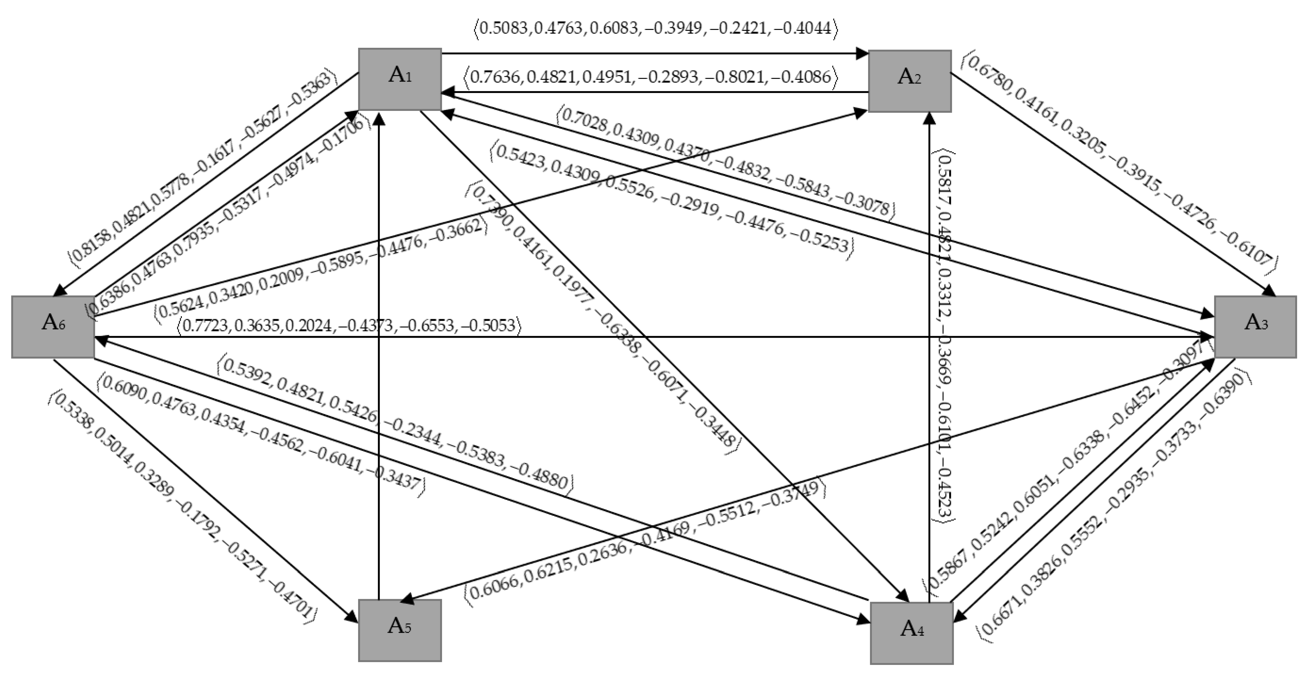
Then, under the condition T p q + 0.5 ( p , q = 1 , 2 , , 6 ) , a partial diagram is drawn, as shown in Figure 4. After that, the out-degree, o u t d ( A p ) ( p = 1 , 2 , , 6 ) of all criteria in a partial directed network are calculated as follows:
o u t d ( A 1 ) = 2.7659 , 2.1391 , 1.8008 , 1.6736 , 1.9962 , 1.5933 o u t d ( A 2 ) = 1.4416 , 0.8982 , 0.8156 , 0.6808 , 1.2747 , 1.0193 o u t d ( A 3 ) = 1.8160 , 1.4350 , 1.3714 , 1.0023 , 1.3721 , 1.5392 o u t d ( A 4 ) = 1.7076 , 1.4884 , 1.4789 , 1.2351 , 1.7936 , 1.2500 o u t d ( A 5 ) = 0.7364 , 0.6073 , 0.4313 , 0.2025 , 0.5450 , 0.4023 o u t d ( A 6 ) = 3.1161 , 2.1595 , 1.9611 , 2.1939 , 2.7315 , 1.8559
According to positive membership degree of out-degree, o u t d ( A p ) ( p = 1 , 2 , , 6 ) , the ranking of the alternatives A p ( p = 1 , 2 , , 6 ) is written as:
A 6 A 1 A 3 A 4 A 2 A 5 .
Therefore, the best alternative is the wind power plant, A 6 .
Now, the elements of the Laplacian matrices of the BSVNDGs, L ( D i ) corresponding to BSVNPRs, M i L ( i = 1 , 2 , 3 ) is given in Table 12, Table 13 and Table 14 while Table 15 presents overall aggregated values.
The Laplacian energy of each BSVNDG D i ( i = 1 , 2 , 3 ) is calculated as:
L E ( D 1 ) = 14.2000 , 15.0000 , 14.2000 , 12.1000 , 15.0000 , 12.1000 , L E ( D 2 ) = 15.5000 , 15.0000 , 15.5000 , 13.2000 , 15.0000 , 13.2000 , L E ( D 3 ) = 14.2000 , 15.0000 , 14.2000 , 12.1000 , 15.0000 , 12.1000 .
Then, the weight of each expert can be determined as:
w i = ( ( w T + ) i , ( w I + ) i , ( w F + ) i , ( w T ) i , ( w I ) i , ( w F ) i ) = ( L E ( ( D T + ) i ) j = 1 k L E ( ( D T + ) j ) , L E ( ( D I + ) i ) j = 1 k L E ( ( D I + ) j ) , L E ( ( D F + ) i ) j = 1 k L E ( ( D F + ) j ) , L E ( ( D T ) i ) j = 1 k L E ( ( D T ) j ) , L E ( ( D I ) i ) j = 1 k L E ( ( D I ) j ) , L E ( ( D F ) i ) j = 1 k L E ( ( D F ) j ) )
where i = 1 , 2 , , k ,
w 1 = 0.3235 , 0.3333 , 0.3235 , 0.3235 , 0.3333 , 0.3235 , w 2 = 0.3531 , 0.3333 , 0.3531 , 0.3529 , 0.3333 , 0.3529 , w 3 = 0.3235 , 0.3333 , 0.3235 , 0.3235 , 0.3333 , 0.3235 .
After that, the out-degree, o u t d ( A p ) ( p = 1 , 2 , , 6 ) of all criteria in a partial directed network are calculated as follows:
o u t d ( A 1 ) = 2.7684 , 1.8053 , 1.8316 , 1.6646 , 1.9985 , 1.5884 o u t d ( A 2 ) = 1.4341 , 0.8981 , 0.8130 , 0.6912 , 1.2758 , 1.0169 o u t d ( A 3 ) = 1.8241 , 1.4350 , 1.3695 , 0.9976 , 1.3742 , 1.5327 o u t d ( A 4 ) = 1.7130 , 1.4883 , 1.4798 , 1.2334 , 1.7948 , 1.2368 o u t d ( A 5 ) = 0.7369 , 0.6073 , 0.4299 , 0.2042 , 0.5421 , 0.4054 o u t d ( A 6 ) = 3.1200 , 2.1594 , 1.9681 , 2.1965 , 2.7229 , 1.8488
According to the positive membership degree of out-degree, o u t d ( A p ) ( p = 1 , 2 , , 6 ) , the ranking of the alternatives A p ( p = 1 , 2 , , 6 ) is given by
A 6 A 1 A 3 A 4 A 2 A 5 .
Therefore, the best alternative is the wind power plant, A 6 .

8. Comparative Study

In this section, the proposed energy BSVNG method is compared with BNSs developed by Deli et al. [30]. First, we construct the pair-wise comparison matrix provided by the decision-maker in Table 8, Table 9 and Table 10. Then, we compute weighted average operators and calculate the score function for each alternative. Lastly, we rank all the alternatives according to the score function. Table 16 shows the score function and rank for each alternative.
Therefore, the ranking of alternatives is given as follows: A 6 A 1 A 3 A 4 A 2 A 5 . As we can see, after the ranking of alternatives according to score function in descending order, A6 is still the best alternative as in our proposed energy BSVNG method. Hence, this comparative method shows the availability and effectiveness of our proposed method.

9. Conclusions

The energy of graphs has many mathematical properties that have been investigated. Certain bounds (upper and lower) on energy had been studied by many researchers. This paper proposed integrating bipolar single-valued neutrosophic set and the energy graph, Laplacian energy graph and signless Laplacian energy graph. Specifically, this paper developed the new concept of energy in BSVNG. It investigated its properties such as the characteristics of eigenvalues, lower and upper bound of energy graph, Laplacian energy graph and signless Laplacian energy graph. Moreover, the relation between them is also discussed, and the proposed method was applied to renewable energy sources selection in which the optimal solution is suggested. In this application, we suggest that a wind power plant (A6) is the optimal alternative. This paper has proceeded with a comparative analysis whereing the rank of alternatives, using the proposed method, is similar to the method of comparison. Hence, it implies that the proposed method is valid and effective. In short, this study implies several significant contributions and modifications to the energy graph, Laplacian energy graph, and signless Laplacian energy graph. In future work, it is suggested to extend the graph energy to: (1) interval-bipolar neutrosophic graphs, (2) neutrosophic vague, (3) dominating energy in neutrosophic graph, etc. Furthermore, this paper does not evaluate the sensitivity of the experts’ weights to the evaluation outcomes. As a result, any new sensitivity analysis, particularly on the experts’ weights, could be pursued as a research topic in the future.

Author Contributions

Conceptualization, S.N.F.M. and R.H.; methodology, S.N.F.M.; software, S.N.F.M.; validation, S.N.F.M., R.H. and B.Y.; formal analysis, S.N.F.M.; investigation, S.N.F.M.; resources, S.N.F.M.; data curation, S.N.F.M.; writing—original draft preparation, S.N.F.M.; writing—review and editing, S.N.F.M., R.H. and B.Y.; visualization, S.N.F.M.; supervision, R.H., F.S. and B.Y.; project administration, R.H.; funding acquisition, R.H. All authors have read and agreed to the published version of the manuscript.

Funding

This research received no external funding.

Institutional Review Board Statement

Not applicable.

Informed Consent Statement

Not applicable.

Data Availability Statement

Not applicable.

Conflicts of Interest

The authors declare no conflict of interest.

References

  1. Gutman, I. The energy of a graph. Ber. Math. Stat. Sekt. Forsch. Graz. 1978, 103, 1–22. [Google Scholar]
  2. Gutman, I.; Zhou, B. Laplacian energy of a graph. Linear Algebra Appl. 2006, 414, 29–37. [Google Scholar] [CrossRef] [Green Version]
  3. Gutman, I. The Energy of a Graph: Old and New Results. Algebraic Combinatorics and Applications; Springer: Berlin/Heidelberg, Germany, 2001; pp. 196–211. [Google Scholar]
  4. Gutman, I.; Kiani, D.; Mirzakhah, M.; Zhou, B. On incidence energy of a graph. Linear Algebra Appl. 2009, 431, 1223–1233. [Google Scholar] [CrossRef] [Green Version]
  5. Zhou, B.; Gutman, I.; Aleksic, T. A note on Laplacian energy of graphs. MATCH Commun. Math. Comput. Chem. 2008, 60, 441–446. [Google Scholar]
  6. Gutman, I.; Wagner, S. The matching energy of a graph. Discret. Appl. Math. 2012, 160, 2177–2187. [Google Scholar] [CrossRef] [Green Version]
  7. So, W.; Robbiano, M.; de Abreu, N.M.M.; Gutman, I. Applications of a theorem by Ky Fan in the theory of graph energy. Linear Algebra Appl. 2010, 432, 2163–2169. [Google Scholar] [CrossRef] [Green Version]
  8. Abreu, N.; Cardoso, D.M.; Gutman, I.; Martins, E.A.; Robbiano, M. Bounds for the signless Laplacian energy. Linear Algebra Appl. 2011, 435, 2365–2374. [Google Scholar] [CrossRef] [Green Version]
  9. Adiga, C.; Bayad, A.; Gutman, I.; Srinivas, S.A. The minimum covering energy of a graph. Kragujev. J. Sci. 2012, 34, 39–54. [Google Scholar]
  10. Das, K.C.; Mojallal, S.A. Relation between energy and (signless) Laplacian energy of graphs. Match 2015, 74, 359–366. [Google Scholar]
  11. Das, K.C.; Mojallal, S.A. Relation between signless Laplacian energy, energy of graph and its line graph. Linear Algebra Appl. 2016, 493, 91–107. [Google Scholar] [CrossRef]
  12. Zadeh, L.A. Fuzzy sets. Inf. Control. 1965, 8, 338–353. [Google Scholar] [CrossRef] [Green Version]
  13. Kauffman, A. Introduction a la Theorie des Sous-Emsembles Flous; Masson et Cie: Paris, France, 1973. [Google Scholar]
  14. Rosenfeld, A. Fuzzy Graph. Fuzzy Sets and Their Applications to Cognitive and Decision Processes; Elsevier: Amsterdam, The Netherlands, 1975; pp. 77–95. [Google Scholar]
  15. Zhang, W.R. Bipolar fuzzy sets and relations: A computational framework for cognitive modeling and multiagent decision analysis. In NAFIPS/IFIS/NASA’94, Proceedings of the First International Joint Conference of the North American Fuzzy Information Processing Society Biannual Conference, the Industrial Fuzzy Control and Intellige; IEEE: Washington, DC, USA, 1995; pp. 305–309. [Google Scholar]
  16. Smarandache, F. A unifying field in logics. In Neutrosophy: Neutrosophic Probability, Set, and Logic; American Research Press: Rehoboth, DE, USA, 1999. [Google Scholar]
  17. Anjali, N.; Mathew, S. Energy of a fuzzy graph. Ann. Fuzzy Math. Inform. 2013, 6, 455–465. [Google Scholar]
  18. Shabaf, S.R.; Fayazi, F. Laplacian Energy of a Fuzzy Graph. Iran. J. Math. Chem. 2014, 5, 1–10. [Google Scholar]
  19. Praba, B.; Chandrasekaran, V.M.; Deepa, G. Energy of an intuitionistic fuzzy graph. Ital. J. Pure Appl. Math. 2014, 32, 431–444. [Google Scholar]
  20. Basha, S.S.; Kartheek, E. Laplacian energy of an intuitionistic fuzzy graph. Indian J. Sci. Technol. 2015, 8, 1–7. [Google Scholar]
  21. Akram, M.; Naz, S. Energy of Pythagorean fuzzy graphs with applications. Mathematics 2018, 6, 136. [Google Scholar] [CrossRef] [Green Version]
  22. Murugesan, R.; Venkatesh, K.A. Laplacian energy of bipolar fuzzy. Int. J. Emerg. Technol. Innov. Res. 2018, 5, 1235–1239. [Google Scholar]
  23. Naz, S.; Ashraf, S.; Karaaslan, F. Energy of a bipolar fuzzy graph and its application in decision making. Ital. J. Pure Appl. Math. 2018, 2018, 339–352. [Google Scholar]
  24. Ramesh, O.; Basha, S.S. The Implementation of Cosine Similarity Measures in Decision-Making Problems by Signless Laplacian Energy of an Intuitionistic Fuzzy Graph. Eur. J. Mol. Clin. Med. 2020, 7, 239–251. [Google Scholar]
  25. Ramesh, O.; Basha, S.S. Group decision making of selecting partner based on signless laplacian energy of an intuitionistic fuzzy graph with topsis method: Study on matlab programming. Adv. Math. Sci. J. 2020, 9, 5849–5859. [Google Scholar] [CrossRef]
  26. Broumi, S.; Talea, M.; Bakali, A.; Singh, P.K.; Broumi, S.; Smarandache, F. Energy and Spectrum Analysis of Interval Valued Neutrosophic Graph using MATLAB. Neutrosophic Sets Syst. 2019, 24, 46–60. [Google Scholar]
  27. Khan, M.; Umar, S.; Broumi, S. Laplacian Energy of a Complex. Neutrosophic Graph; Springer: Cham, Switzerland, 2019; pp. 203–232. [Google Scholar]
  28. Naz, S.; Akram, M.; Smarandache, F. Certain Notions of Energy in Single-Valued Neutrosophic Graphs. Axioms 2018, 7, 50. [Google Scholar] [CrossRef] [Green Version]
  29. Mullai, M.; Broumi, S. Dominating Energy in Neutrosophic graphs. Int. J. Neutrosoph. Sci. 2020, 5, 38–58. [Google Scholar]
  30. Deli, I.; Ali, M.; Smarandache, F. Bipolar Neutrosophic Sets And Their Application Based On Multi-Criteria Decision Making Problems. In Proceedings of the 2015 International Conference on Advanced Mechatronic Systems, Beijing, China, 22–24 August 2015. [Google Scholar]
  31. Broumi, S.; Smarandache, F.; Talea, M.; Bakali, A. An Introduction to Bipolar Single Valued Neutrosophic Graph Theory. Appl. Mech. Mater. 2016, 841, 184–191. [Google Scholar] [CrossRef] [Green Version]
  32. Broumi, S.; Talea, M.; Bakali, A.; Smarandache, F. On Bipolar Single Valued Neutrosophic Graphs. J. New Theory 2016, 11, 84–102. [Google Scholar]
  33. Ali, M.; Son, L.H.; Deli, I.; Tien, N.D. Bipolar neutrosophic soft sets and applications in decision making. J. Intell. Fuzzy Syst. 2017, 33, 4077–4087. [Google Scholar] [CrossRef] [Green Version]
  34. Akram, M.; Luqman, A. A new decision-making method based on bipolar neutrosophic directed hypergraphs. J. Appl. Math. Comput. 2018, 57, 547–575. [Google Scholar] [CrossRef]
  35. Akram, M.; Shumaiza; Smarandache, F. Decision-making with bipolar neutrosophic TOPSIS and bipolar neutrosophic ELECTRE-I. Axioms 2018, 7, 33. [Google Scholar] [CrossRef] [Green Version]
  36. Uluçay, V.; Deli, I.; Şahin, M. Similarity measures of bipolar neutrosophic sets and their application to multiple criteria decision making. Neural Comput. Appl. 2018, 29, 739–748. [Google Scholar] [CrossRef] [Green Version]
  37. Abdel-Basset, M.; Mohamed, M.; Elhoseny, M.; Son, L.H.; Chiclana, F.; Zaied, A.E.N.H. Cosine similarity measures of bipolar neutrosophic set for diagnosis of bipolar disorder diseases. Artif. Intell. Med. 2019, 101, 101735. [Google Scholar] [CrossRef] [PubMed]
  38. Fan, C.; Ye, J.; Feng, S.; Fan, E.; Hu, K. Multi-criteria decision-making method using heronian mean operators under a bipolar neutrosophic environment. Mathematics 2019, 7, 97. [Google Scholar] [CrossRef] [Green Version]
  39. Abdel-Basset, M.; Gamal, A.; Son, L.H.; Smarandache, F. A bipolar neutrosophic multi criteria decision making framework for professional selection. Appl. Sci. 2020, 10, 1202. [Google Scholar] [CrossRef] [Green Version]
  40. Rahim, N.; Abdullah, L.; Yusoff, B. A border approximation area approach considering bipolar neutrosophic linguistic variable for sustainable energy selection. Sustainability 2020, 12, 3971. [Google Scholar] [CrossRef]
  41. Karaşan, A.; Kahraman, C. Selection of the Most Appropriate Renewable Energy Alternatives by Using a Novel Interval-Valued Neutrosophic ELECTRE I Method. Informatica 2020, 31, 225–248. [Google Scholar] [CrossRef] [Green Version]
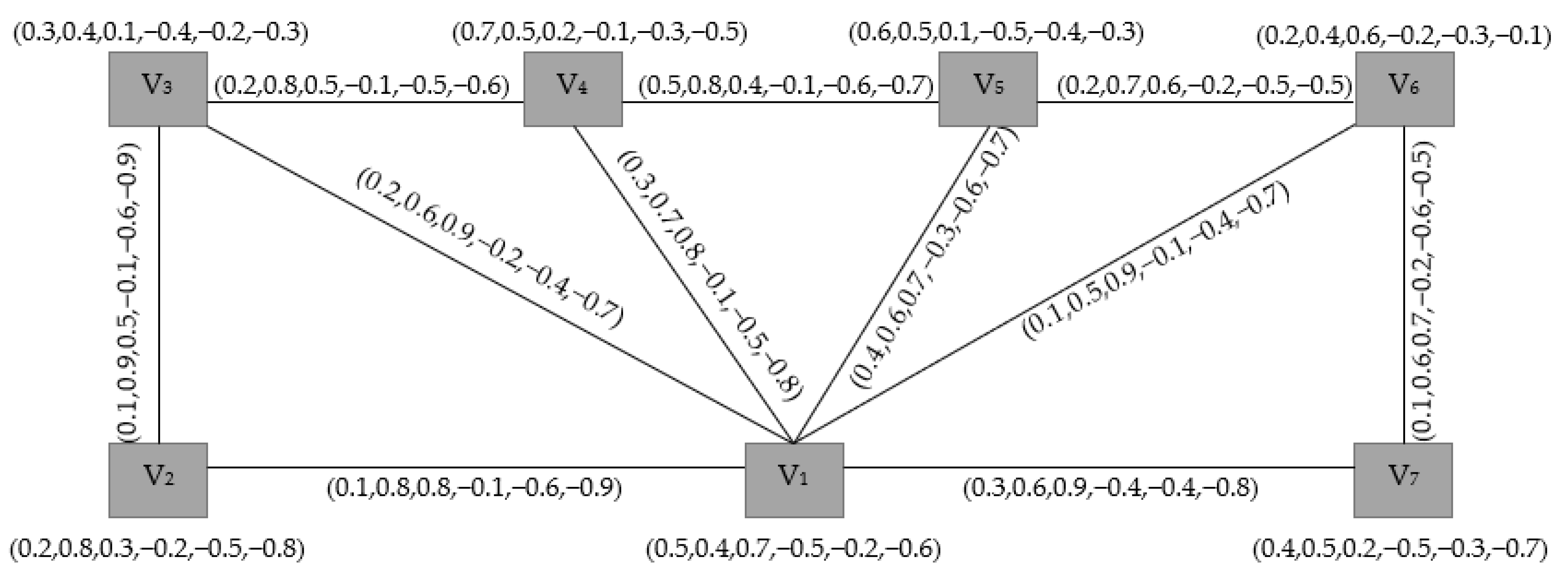
Figure 1. The energy of a bipolar single-valued neutrosophic graph.
Axioms 10 00172 g001
Figure 2. Laplacian energy a of bipolar single-valued neutrosophic graph.
Axioms 10 00172 g002
Figure 3. Signless Laplacian energy of a bipolar single-valued neutrosophic graph.
Axioms 10 00172 g003
Figure 4. Partial directed network of the BSVN.
Axioms 10 00172 g004
Table 1. Significance influences towards energy, Laplacian energy and signless Laplacian energy graph.
Author and ReferencesYearFuzzy/Neutrosophic SetsSignificance Influences
Akram and Naz [21]2018Pythagorean fuzzy setsIntroduce the energy and Laplacian energy in Pythagorean fuzzy graphs and Pythagorean fuzzy digraphs.
Rajeshwari et al. [22]2018Bipolar fuzzy setsIntroduce Laplacian energy for a bipolar fuzzy graph.
Naz et al. [23]2018Bipolar fuzzy setsIntroduce the concept of energy in bipolar fuzzy graph (BFG) and bipolar fuzzy digraphs (BFDGs).
Naz et al. [28]2018Single-valued neutrosophic setsIntroduce the concept of energy, Laplacian energy and signless Laplacian energy in single-valued neutrosophic graphs (SVNGs).
Broumi et al. [26]2019Interval-valued neutrosophic setsCompute the spectrum and energy of interval-valued neutrosophic graph (IVNG).
Mohsin et al. [27]2019Complex neutrosophic setCompute Laplacian energy of a complex neutrosophic graph in terms of its adjacency matrix.
Ramesh and Basha [24]2020Intuitionistic fuzzy setsSolve decision-making problem by signless Laplacian energy of intuitionistic fuzzy graph and cosine similarity measure.
Ramesh and Basha [25]2020Intuitionistic fuzzy setsSolve group decision-making problem by signless Laplacian energy of intuitionistic fuzzy graph.
Mullai and Broumi [29]2020Single-valued neutrosophic setsIntroduce dominating sets and dominating numbers for energy graphs in single-valued neutrosophic graphs.
Table 2. The energy of BSVNG set on V.
α v 1 v 2 v 3 v 4 v 5 v 6 v 7
T α + 0.50.20.30.70.60.20.4
I α + 0.40.80.40.50.50.40.5
F α + 0.70.30.10.20.10.60.2
T α −0.5−0.2−0.4−0.1−0.5−0.2−0.5
I α −0.2−0.5−0.2−0.3−0.4−0.3−0.3
F α −0.6−0.8−0.3−0.5−0.3−0.1−0.7
Table 3. The energy of BSVNG relation on V.
β v 1 v 2 v 1 v 3 v 1 v 4 v 1 v 5 v 1 v 6 v 1 v 7 v 2 v 3 v 3 v 4 v 4 v 5 v 5 v 6 v 6 v 7
T β + 0.10.20.30.40.10.30.10.20.50.20.1
I β + 0.80.60.70.60.50.60.90.80.80.70.6
F β + 0.80.90.80.70.90.90.50.50.40.60.7
T β −0.1−0.2−0.1−0.3−0.1−0.4−0.1−0.1−0.1−0.2−0.2
I β −0.6−0.4−0.5−0.6−0.4−0.4−0.6−0.5−0.6−0.5−0.6
F β −0.9−0.7−0.8−0.7−0.7−0.8−0.9−0.6−0.7−0.5−0.5
Table 4. Laplacian energy of BSVNG set on V.
α v 1 v 2 v 3 v 4 v 5 v 6 v 7
T α + 0.30.20.40.20.10.40.5
I α + 0.60.70.80.50.50.30.5
F α + 0.40.60.30.70.80.50.8
T α −0.3−0.4−0.2−0.5−0.1−0.2−0.6
I α −0.5−0.6−0.4−0.2−0.5−0.4−0.7
F α −0.8−0.7−0.6−0.4−0.6−0.5−0.9
Table 5. Laplacian energy of BSVNG relation on V.
β v 1 v 2 v 1 v 6 v 1 v 7 v 2 v 3 v 2 v 7 v 3 v 4 v 3 v 7 v 4 v 5 v 4 v 7 v 5 v 6 v 5 v 7 v 6 v 7
T β + 0.10.20.20.10.20.10.30.10.20.10.10.4
I β + 0.80.70.70.90.80.90.80.60.70.50.70.6
F β + 0.60.80.90.70.90.80.90.80.90.80.90.8
T β −0.2−0.1−0.2−0.2−0.4−0.2−0.2−0.1−0.3−0.1−0.1−0.2
I β −0.7−0.9−0.8−0.6−0.7−0.5−0.8−0.6−0.8−0.6−0.8−0.8
F β −0.9 −0.8−0.9−0.7−0.9−0.6−0.9−0.7−0.9−0.6−0.9−0.9
Table 6. Signless Laplacian energy of BSVNG set on V.
α v 1 v 2 v 3 v 4 v 5 v 6 v 7
T α + 0.20.70.10.50.30.40.8
I α + 0.60.10.30.20.40.60.7
F α + 0.40.50.20.10.70.70.6
T α −0.4−0.1−0.3−0.4−0.5−0.2−0.5
I α −0.6−0.3−0.2−0.5−0.3−0.4−0.4
F α −0.1−0.6−0.5−0.2−0.4−0.1−0.3
Table 7. Signless Laplacian energy of BSVNG relation on V.
β v 1 v 2 v 1 v 3 v 2 v 3 v 2 v 4 v 2 v 5 v 3 v 5 v 4 v 5 v 4 v 6 v 4 v 7 v 5 v 7 v 6 v 7
T β + 0.20.10.10.40.30.10.20.30.40.20.3
I β + 0.70.60.40.30.50.50.50.70.80.80.7
F β + 0.60.50.60.70.80.80.70.80.60.80.8
T β −0.1−0.2−0.1−0.1−0.1−0.3−0.3−0.2−0.3−0.4−0.1
I β −0.8−0.7−0.4−0.6−0.4−0.5−0.6−0.7−0.5−0.5−0.6
F β −0.7−0.5−0.6−0.8−0.7−0.5−0.4−0.3−0.4−0.5−0.4
Table 8. BSVNPR of the expert from the operation management department.
M 1 A 1 A 2 A 3 A 4 A 5 A 6
A 1 0.5 , 0.5 , 0.5 , 0.5 , 0.5 , 0.5 0.4 , 0.6 , 0.3 , 0.3 , 0.1 , 0.4 0.3 , 0.2 , 0.6 , 0.4 , 0.6 , 0.2 0.7 , 0.3 , 0.4 , 0.6 , 0.5 , 0.3 0.4 , 0.2 , 0.8 , 0.5 , 0.3 , 0.2 0.9 , 0.4 , 0.6 , 0.1 , 0.6 , 0.5
A 2 0.3 , 0.4 , 0.4 , 0.4 , 0.9 , 0.3 0.5 , 0.5 , 0.5 , 0.5 , 0.5 , 0.5 0.8 , 0.3 , 0.2 , 0.5 , 0.2 , 0.6 0.3 , 0.2 , 0.7 , 0.2 , 0.3 , 0.5 0.4 , 0.2 , 0.3 , 0.2 , 0.5 , 0.7 0.2 , 0.5 , 0.6 , 0.4 , 0.6 , 0.7
A 3 0.6 , 0.8 , 0.3 , 0.2 , 0.4 , 0.4 0.2 , 0.7 , 0.8 , 0.6 , 0.8 , 0.5 0.5 , 0.5 , 0.5 , 0.5 , 0.5 , 0.5 0.8 , 0.2 , 0.4 , 0.2 , 0.3 , 0.6 0.3 , 0.5 , 0.2 , 0.5 , 0.5 , 0.2 0.1 , 0.4 , 0.7 , 0.5 , 0.2 , 0.6
A 4 0.4 , 0.7 , 0.7 , 0.3 , 0.5 , 0.6 0.7 , 0.8 , 0.3 , 0.5 , 0.7 , 0.2 0.4 , 0.8 , 0.8 , 0.6 , 0.7 , 0.2 0.5 , 0.5 , 0.5 , 0.5 , 0.5 , 0.5 0.3 , 0.2 , 0.1 , 0.6 , 0.3 , 0.4 0.7 , 0.4 , 0.5 , 0.1 , 0.2 , 0.3
A 5 0.8 , 0.8 , 0.4 , 0.2 , 0.7 , 0.5 0.3 , 0.8 , 0.4 , 0.7 , 0.5 , 0.2 0.2 , 0.5 , 0.3 , 0.2 , 0.5 , 0.5 0.1 , 0.8 , 0.3 , 0.4 , 0.7 , 0.6 0.5 , 0.5 , 0.5 , 0.5 , 0.5 , 0.5 0.4 , 0.3 , 0.8 , 0.6 , 0.3 , 0.2
A 6 0.6 , 0.6 , 0.9 , 0.5 , 0.4 , 0.1 0.6 , 0.5 , 0.2 , 0.7 , 0.4 , 0.4 0.7 , 0.6 , 0.1 , 0.6 , 0.8 , 0.5 0.5 , 0.6 , 0.7 , 0.3 , 0.8 , 0.1 0.8 , 0.7 , 0.4 , 0.2 , 0.7 , 0.6 0.5 , 0.5 , 0.5 , 0.5 , 0.5 , 0.5
Table 9. BSVNPR of the expert from the engineering management department.
M 2 A 1 A 2 A 3 A 4 A 5 A 6
A 1 0.5 , 0.5 , 0.5 , 0.5 , 0.5 , 0.5 0.5 , 0.3 , 0.8 , 0.4 , 0.2 , 0.6 0.9 , 0.8 , 0.7 , 0.4 , 0.7 , 0.3 0.8 , 0.4 , 0.2 , 0.7 , 0.4 , 0.2 0.4 , 0.3 , 0.7 , 0.4 , 0.4 , 0.4 0.7 , 0.4 , 0.8 , 0.2 , 0.3 , 0.5
A 2 0.8 , 0.7 , 0.5 , 0.6 , 0.8 , 0.4 0.5 , 0.5 , 0.5 , 0.5 , 0.5 , 0.5 0.2 , 0.3 , 0.4 , 0.6 , 0.4 , 0.7 0.4 , 0.3 , 0.6 , 0.3 , 0.4 , 0.5 0.3 , 0.4 , 0.6 , 0.4 , 0.6 , 0.7 0.4 , 0.6 , 0.7 , 0.3 , 0.4 , 0.5
A 3 0.7 , 0.2 , 0.9 , 0.3 , 0.3 , 0.4 0.4 , 0.7 , 0.2 , 0.7 , 0.6 , 0.6 0.5 , 0.5 , 0.5 , 0.5 , 0.5 , 0.5 0.7 , 0.4 , 0.6 , 0.4 , 0.3 , 0.7 0.7 , 0.6 , 0.3 , 0.3 , 0.4 , 0.6 0.2 , 0.6 , 0.8 , 0.4 , 0.3 , 0.7
A 4 0.2 , 0.6 , 0.8 , 0.2 , 0.6 , 0.7 0.6 , 0.7 , 0.4 , 0.5 , 0.6 , 0.3 0.6 , 0.6 , 0.7 , 0.7 , 0.7 , 0.4 0.5 , 0.5 , 0.5 , 0.5 , 0.5 , 0.5 0.4 , 0.4 , 0.2 , 0.3 , 0.4 , 0.4 0.6 , 0.4 , 0.4 , 0.2 , 0.4 , 0.6
A 5 0.7 , 0.7 , 0.4 , 0.4 , 0.6 , 0.4 0.6 , 0.6 , 0.3 , 0.7 , 0.4 , 0.4 0.3 , 0.4 , 0.7 , 0.6 , 0.6 , 0.3 0.2 , 0.6 , 0.4 , 0.4 , 0.6 , 0.3 0.5 , 0.5 , 0.5 , 0.5 , 0.5 , 0.5 0.3 , 0.7 , 0.2 , 0.4 , 0.4 , 0.1
A 6 0.8 , 0.6 , 0.7 , 0.5 , 0.7 , 0.2 0.7 , 0.4 , 0.4 , 0.5 , 0.6 , 0.3 0.8 , 0.4 , 0.2 , 0.7 , 0.7 , 0.4 0.4 , 0.6 , 0.6 , 0.6 , 0.6 , 0.2 0.2 , 0.3 , 0.3 , 0.1 , 0.6 , 0.4 0.5 , 0.5 , 0.5 , 0.5 , 0.5 , 0.5
Table 10. BSVNPR of the expert from the human resource department.
M 3 A 1 A 2 A 3 A 4 A 5 A 6
A 1 0.5 , 0.5 , 0.5 , 0.5 , 0.5 , 0.5 0.6 , 0.6 , 0.9 , 0.5 , 0.4 , 0.1 0.6 , 0.5 , 0.2 , 0.7 , 0.4 , 0.4 0.7 , 0.6 , 0.1 , 0.6 , 0.8 , 0.5 0.5 , 0.6 , 0.7 , 0.3 , 0.8 , 0.1 0.8 , 0.7 , 0.4 , 0.2 , 0.7 , 0.6
A 2 0.9 , 0.4 , 0.6 , 0.1 , 0.6 , 0.5 0.5 , 0.5 , 0.5 , 0.5 , 0.5 , 0.5 0.8 , 0.8 , 0.4 , 0.2 , 0.7 , 0.5 0.3 , 0.8 , 0.4 , 0.7 , 0.5 , 0.2 0.2 , 0.5 , 0.3 , 0.2 , 0.5 , 0.5 0.1 , 0.8 , 0.3 , 0.4 , 0.7 , 0.6
A 3 0.2 , 0.5 , 0.6 , 0.4 , 0.6 , 0.7 0.4 , 0.2 , 0.8 , 0.5 , 0.3 , 0.2 0.5 , 0.5 , 0.5 , 0.5 , 0.5 , 0.5 0.4 , 0.7 , 0.7 , 0.3 , 0.5 , 0.6 0.7 , 0.8 , 0.3 , 0.5 , 0.7 , 0.2 0.4 , 0.8 , 0.8 , 0.6 , 0.7 , 0.2
A 4 0.1 , 0.4 , 0.7 , 0.5 , 0.2 , 0.6 0.4 , 0.2 , 0.3 , 0.2 , 0.5 , 0.7 0.7 , 0.3 , 0.4 , 0.6 , 0.5 , 0.3 0.5 , 0.5 , 0.5 , 0.5 , 0.5 , 0.5 0.6 , 0.8 , 0.3 , 0.2 , 0.4 , 0.4 0.2 , 0.7 , 0.8 , 0.6 , 0.8 , 0.5
A 5 0.7 , 0.4 , 0.5 , 0.1 , 0.2 , 0.3 0.3 , 0.5 , 0.2 , 0.5 , 0.5 , 0.2 0.3 , 0.2 , 0.7 , 0.2 , 0.3 , 0.5 0.3 , 0.2 , 0.6 , 0.4 , 0.6 , 0.2 0.5 , 0.5 , 0.5 , 0.5 , 0.5 , 0.5 0.3 , 0.4 , 0.4 , 0.4 , 0.9 , 0.3
A 6 0.4 , 0.3 , 0.8 , 0.6 , 0.3 , 0.2 0.3 , 0.2 , 0.1 , 0.6 , 0.3 , 0.4 0.8 , 0.2 , 0.4 , 0.2 , 0.3 , 0.6 0.8 , 0.3 , 0.2 , 0.5 , 0.2 , 0.6 0.4 , 0.6 , 0.3 , 0.3 , 0.1 , 0.4 0.5 , 0.5 , 0.5 , 0.5 , 0.5 , 0.5
Table 11. The collective BSVNPR of all the above individual BSVNPRs.
MA1A2A3
A1 0.5000 , 0.5000 , 0.5000 , 0.5000 , 0.5000 , 0.5000 0.5083 , 0.4763 , 0.6083 , 0.3949 , 0.2421 , 0.4044 0.7028 , 0.4309 , 0.4370 0.4832 , 0.5843 , 0.3078
A2 0.7636 , 0.4821 , 0.4951 , 0.2893 , 0.8021 , 0.4086 0.5000 , 0.5000 , 0.5000 , 0.5000 , 0.5000 , 0.5000 0.6780 , 0.4161 , 0.3205 , 0.3915 , 0.4726 , 0.6107
A3 0.5423 , 0.4309 , 0.5526 , 0.2919 , 0.4476 , 0.5253 0.3422 , 0.4611 , 0.4970 , 0.5959 , 0.6211 , 0.4587 0.5000 , 0.5000 , 0.5000 , 0.5000 , 0.5000 , 0.5000
A4 0.2407 , 0.5518 , 0.7329 , 0.3086 , 0.4578 , 0.6390 0.5817 , 0.4821 , 0.3312 , 0.3669 , 0.6101 , 0.4523 0.5867 , 0.5242 , 0.6051 , 0.6338 , 0.6452 , 0.3097
A5 0.7364 , 0.6073 , 0.4313 , 0.2025 , 0.5450 , 0.4023 0.4224 , 0.6215 , 0.2870 , 0.6248 , 0.4692 , 0.2779 0.2694 , 0.3420 , 0.5339 , 0.2956 , 0.4811 , 0.4365
A6 0.6386 , 0.4763 , 0.7935 , 0.5317 , 0.4974 , 0.1706 0.5624 , 0.3420 , 0.2009 , 0.5895 , 0.4476 , 0.3662 0.7723 , 0.3635 , 0.2024 , 0.4373 , 0.6553 , 0.5053
A4A5A6
A1 0.7390 , 0.4161 , 0.1977 , 0.6338 , 0.6071 , 0.3448 0.4357 , 0.3302 , 0.7306 , 0.3886 , 0.5590 , 0.2485 0.8158 , 0.4821 , 0.5778 , 0.1617 , 0.5627 , 0.5363
A2 0.3361 , 0.3635 , 0.5499 , 0.3527 , 0.4042 , 0.4140 0.3030 , 0.3420 , 0.3807 , 0.2559 , 0.5354 , 0.6435 0.2459 , 0.6215 , 0.5009 , 0.3610 , 0.5843 , 0.6035
A3 0.6671 , 0.3826 , 0.5552 , 0.2935 , 0.3733 , 0.6390 0.6066 , 0.6215 , 0.2636 , 0.4169 , 0.5512 , 0.3749 0.2460 , 0.5769 , 0.7666 , 0.4911 , 0.4452 , 0.5437
A4 0.5000 , 0.5000 , 0.5000 , 0.5000 , 0.5000 , 0.5000 0.4501 , 0.4000 , 0.1837 , 0.3235 , 0.3674 , 0.4000 0.5392 , 0.4821 , 0.5426 , 0.2344 , 0.5383 , 0.4880
A5 0.2058 , 0.4579 , 0.4183 , 0.4000 , 0.6376 , 0.3831 0.5000 , 0.5000 , 0.5000 , 0.5000 , 0.5000 , 0.5000 0.3336 , 0.4380 , 0.3935 , 0.4529 , 0.6488 , 0.2026
A6 0.6090 , 0.4763 , 0.4354 , 0.4562 , 0.6041 , 0.3437 0.5338 , 0.5014 , 0.3289 , 0.1792 , 0.5271 , 0.4701 0.5000 , 0.5000 , 0.5000 , 0.5000 , 0.5000 , 0.5000
Table 12. Elements of the Laplacian matrix of the BSVNDG, D 1 .
M 1 A 1 A 2 A 3 A 4 A 5 A 6
A1 2.7 , 1.7 , 2.7 , 1.9 , 2.1 , 1.6 0.4 , 0.6 , 0.3 , 0.3 , 0.1 , 0.4 0.3 , 0.2 , 0.6 , 0.4 , 0.6 , 0.2 0.7 , 0.3 , 0.4 , 0.6 , 0.5 , 0.3 0.4 , 0.2 , 0.8 , 0.5 , 0.3 , 0.2 0.9 , 0.4 , 0.6 , 0.1 , 0.6 , 0.5
A2 0.3 , 0.4 , 0.4 , 0.4 , 0.9 , 0.3 2.0 , 1.6 , 2.2 , 1.7 , 2.5 , 2.8 0.8 , 0.3 , 0.2 , 0.5 , 0.2 , 0.6 0.3 , 0.2 , 0.7 , 0.2 , 0.3 , 0.5 0.4 , 0.2 , 0.3 , 0.2 , 0.5 , 0.7 0.2 , 0.5 , 0.6 , 0.4 , 0.6 , 0.7
A3 0.6 , 0.8 , 0.3 , 0.2 , 0.4 , 0.4 0.2 , 0.7 , 0.8 , 0.6 , 0.8 , 0.5 2.0 , 2.6 , 2.4 , 2.0 , 2.2 , 2.3 0.8 , 0.2 , 0.4 , 0.2 , 0.3 , 0.6 0.3 , 0.5 , 0.2 , 0.5 , 0.5 , 0.2 0.1 , 0.4 , 0.7 , 0.5 , 0.2 , 0.6
A4 0.4 , 0.7 , 0.7 , 0.3 , 0.5 , 0.6 0.7 , 0.8 , 0.3 , 0.5 , 0.7 , 0.2 0.4 , 0.8 , 0.8 , 0.6 , 0.7 , 0.2 2.5 , 2.9 , 2.4 , 2.1 , 2.4 , 1.7 0.3 , 0.2 , 0.1 , 0.6 , 0.3 , 0.4 0.7 , 0.4 , 0.5 , 0.1 , 0.2 , 0.3
A5 0.8 , 0.8 , 0.4 , 0.2 , 0.7 , 0.5 0.3 , 0.8 , 0.4 , 0.7 , 0.5 , 0.2 0.2 , 0.5 , 0.3 , 0.2 , 0.5 , 0.5 0.1 , 0.8 , 0.3 , 0.4 , 0.7 , 0.6 1.8 , 3.2 , 2.2 , 2.1 , 2.7 , 2.0 0.4 , 0.3 , 0.8 , 0.6 , 0.3 , 0.2
A6 0.6 , 0.6 , 0.9 , 0.5 , 0.4 , 0.1 0.6 , 0.5 , 0.2 , 0.7 , 0.4 , 0.4 0.7 , 0.6 , 0.1 , 0.6 , 0.8 , 0.5 0.5 , 0.6 , 0.7 , 0.3 , 0.8 , 0.1 0.8 , 0.7 , 0.4 , 0.2 , 0.7 , 0.6 3.2 , 3.0 , 2.3 , 2.3 , 3.1 , 1.7
Table 13. Elements of the Laplacian matrix of the BSVNDG, D 2 .
M 2 A 1 A 2 A 3 A 4 A 5 A 6
A1 3.3 , 2.2 , 3.2 , 2.1 , 2.0 , 2.0 0.5 , 0.3 , 0.8 , 0.4 , 0.2 , 0.6 0.9 , 0.8 , 0.7 , 0.4 , 0.7 , 0.3 0.8 , 0.4 , 0.2 , 0.7 , 0.4 , 0.2 0.4 , 0.3 , 0.7 , 0.4 , 0.4 , 0.4 0.7 , 0.4 , 0.8 , 0.2 , 0.3 , 0.5
A2 0.8 , 0.7 , 0.5 , 0.6 , 0.8 , 0.4 2.1 , 2.3 , 2.8 , 2.2 , 2.6 , 2.8 0.2 , 0.3 , 0.4 , 0.6 , 0.4 , 0.7 0.4 , 0.3 , 0.6 , 0.3 , 0.4 , 0.5 0.3 , 0.4 , 0.6 , 0.4 , 0.6 , 0.7 0.4 , 0.6 , 0.7 , 0.3 , 0.4 , 0.5
A3 0.7 , 0.2 , 0.9 , 0.3 , 0.3 , 0.4 0.4 , 0.7 , 0.2 , 0.7 , 0.6 , 0.6 0.4 , 0.7 , 0.2 , 0.7 , 0.6 , 0.6 0.7 , 0.4 , 0.6 , 0.4 , 0.3 , 0.7 0.7 , 0.6 , 0.3 , 0.3 , 0.4 , 0.6 0.2 , 0.6 , 0.8 , 0.4 , 0.3 , 0.7
A4 0.2 , 0.6 , 0.8 , 0.2 , 0.6 , 0.7 0.6 , 0.7 , 0.4 , 0.5 , 0.6 , 0.3 0.6 , 0.6 , 0.7 , 0.7 , 0.7 , 0.4 2.4 , 2.7 , 2.5 , 1.9 , 2.7 , 2.4 0.4 , 0.4 , 0.2 , 0.3 , 0.4 , 0.4 0.6 , 0.4 , 0.4 , 0.2 , 0.4 , 0.6
A5 0.7 , 0.7 , 0.4 , 0.4 , 0.6 , 0.4 0.6 , 0.6 , 0.3 , 0.7 , 0.4 , 0.4 0.3 , 0.4 , 0.7 , 0.6 , 0.6 , 0.3 0.2 , 0.6 , 0.4 , 0.4 , 0.6 , 0.3 2.1 , 3.0 , 2.0 , 2.5 , 2.6 , 1.5 0.3 , 0.7 , 0.2 , 0.4 , 0.4 , 0.1
A6 0.8 , 0.6 , 0.7 , 0.5 , 0.7 , 0.2 0.7 , 0.4 , 0.4 , 0.5 , 0.6 , 0.3 0.8 , 0.4 , 0.2 , 0.7 , 0.7 , 0.4 0.4 , 0.6 , 0.6 , 0.6 , 0.6 , 0.2 0.2 , 0.3 , 0.3 , 0.1 , 0.6 , 0.4 2.9 , 2.3 , 2.2 , 2.4 , 3.2 , 1.5
Table 14. Elements of the Laplacian matrix of the BSVNDG, D 3 .
M 3 A 1 A 2 A 3 A 4 A 5 A 6
A1 3.2 , 3.0 , 2.3 , 2.3 , 3.1 , 1.7 0.6 , 0.6 , 0.9 , 0.5 , 0.4 , 0.1 0.6 , 0.5 , 0.2 , 0.7 , 0.4 , 0.4 0.7 , 0.6 , 0.1 , 0.6 , 0.8 , 0.5 0.5 , 0.6 , 0.7 , 0.3 , 0.8 , 0.1 0.8 , 0.7 , 0.4 , 0.2 , 0.7 , 0.6
A2 0.9 , 0.4 , 0.6 , 0.1 , 0.6 , 0.5 2.3 , 3.3 , 2.0 , 1.6 , 3.0 , 2.3 0.8 , 0.8 , 0.4 , 0.2 , 0.7 , 0.5 0.3 , 0.8 , 0.4 , 0.7 , 0.5 , 0.2 0.2 , 0.5 , 0.3 , 0.2 , 0.5 , 0.5 0.1 , 0.8 , 0.3 , 0.4 , 0.7 , 0.6
A3 0.2 , 0.5 , 0.6 , 0.4 , 0.6 , 0.7 0.4 , 0.2 , 0.8 , 0.5 , 0.3 , 0.2 2.1 , 3.0 , 3.2 , 2.3 , 2.8 , 1.9 0.4 , 0.7 , 0.7 , 0.3 , 0.5 , 0.6 0.7 , 0.8 , 0.3 , 0.5 , 0.7 , 0.2 0.4 , 0.8 , 0.8 , 0.6 , 0.7 , 0.2
A4 0.1 , 0.4 , 0.7 , 0.5 , 0.2 , 0.6 0.4 , 0.2 , 0.3 , 0.2 , 0.5 , 0.7 0.7 , 0.3 , 0.4 , 0.6 , 0.5 , 0.3 2.0 , 2.4 , 2.5 , 2.1 , 2.4 , 2.5 0.6 , 0.8 , 0.3 , 0.2 , 0.4 , 0.4 0.2 , 0.7 , 0.8 , 0.6 , 0.8 , 0.5
A5 0.7 , 0.4 , 0.5 , 0.1 , 0.2 , 0.3 0.3 , 0.5 , 0.2 , 0.5 , 0.5 , 0.2 0.3 , 0.2 , 0.7 , 0.2 , 0.3 , 0.5 0.3 , 0.2 , 0.6 , 0.4 , 0.6 , 0.2 1.9 , 1.7 , 2.4 , 1.6 , 2.5 , 1.5 0.3 , 0.4 , 0.4 , 0.4 , 0.9 , 0.3
A6 0.4 , 0.3 , 0.8 , 0.6 , 0.3 , 0.2 0.3 , 0.2 , 0.1 , 0.6 , 0.3 , 0.4 0.8 , 0.2 , 0.4 , 0.2 , 0.3 , 0.6 0.8 , 0.3 , 0.2 , 0.5 , 0.2 , 0.6 0.4 , 0.6 , 0.3 , 0.3 , 0.1 , 0.4 2.7 , 1.6 , 1.8 , 2.2 , 1.2 , 2.2
Table 15. The collective BSVNPR of all the above individual BSVNPRs.
MA1A2A3
A1 0.5000 , 0.5000 , 0.5000 , 0.5000 , 0.5000 , 0.5000 0.5066 , 0.4763 , 0.6051 , 0.3918 , 0.2440 , 0.4071 0.7062 , 0.4309 , 0.4440 , 0.4794 , 0.5839 , 0.3046
A2 0.7603 , 0.4821 , 0.4934 , 0.2948 , 0.8000 , 0.4054 0.5000 , 0.5000 , 0.5000 , 0.5000 , 0.5000 , 0.5000 0.6738 , 034161 , 0.3196 , 0.3965 , 0.4758 , 0.6115
A3 0.5478 , 0.4309 , 0.5533 , 0.2888 , 0.4482 , 0.5205 0.3415 , 0.4611 , 0.4903 , 0.5973 , 0.6174 , 0.4619 0.5000 , 0.5000 , 0.5000 , 0.5000 , 0.5000 , 0.5000
A4 0.2428 , 0.5518 , 0.7338 , 0.3068 , 0.4571 , 0.6386 0.5845 , 0.4821 , 0.3320 , 0.3718 , 0.6085 , 0.4443 0.5845 , 0.5242 , 0.6098 , 0.6336 , 0.6443 , 0.3078
A5 0.7369 , 0.6073 , 0.4299 , 0.2042 , 0.5421 , 0.4054 0.4255 , 0.6215 , 0.2887 , 0.6278 0.4686 , 0.2772 0.2691 , 0.3420 , 0.5322 , 0.2948 , 0.4807 , 0.4369
A6 0.6430 , 0.4763 , 0.7928 , 0.5304 , 0.4986 , 0.1689 0.5670 , 0.3420 , 0.2041 , 0.5914 , 0.4482 , 0.3664 0.7720 , 0.3635 , 0.2000 , 0.4441 , 0.6524 , 0.5039
A4A5A6
A1 0.7400 , 0.4161 , 0.2000 , 0.6336 , 0.6085 , 0.3419 0.4344 , 0.3302 , 0.7309 , 0.3918 , 0.5620 , 0.2491 0.8156 , 0.4821 , 0.5825 , 0.1599 , 0.5620 , 0.5348
A2 0.3371 , 0.3635 , 0.5531 , 0.3461 , 0.4056 , 0.4179 0.3047 , 0.3420 , 0.3831 , 0.2555 , 0.5358 , 0.6461 0.2492 , 0.6215 , 0.5063 , 0.3614 , 0.5839 , 0.6057
A3 0.6708 , 0.3826 , 0.5531 , 0.2913 , 0.3742 , 0.6386 0.6054 , 0.6215 , 0.2631 , 0.4176 , 0.5518 , 0.3736 0.2428 , 0.5769 , 0.7662 , 0.4902 , 0.4482 , 0.5477
A4 0.5000 , 0.5000 , 0.5000 , 0.5000 , 0.5000 , 0.5000 0.4469 , 0.4000 , 0.1822 , 0.3293 , 0.3683 , 0.4000 0.5440 , 0.4821 , 0.5380 , 0.2281 , 0.5421 , 0.4847
A5 0.2041 , 0.4579 , 0.4155 , 0.4000 , 0.6365 , 0.3901 0.5000 , 0.5000 , 0.5000 , 0.5000 , 0.5000 , 0.5000 0.3341 , 0.4380 , 0.3918 , 0.4561 , 0.6524 , 0.2013
A6 0.6036 , 0.4763 , 0.4420 , 0.4520 , 0.6000 , 0.3359 0.5345 , 0.5014 , 0.3292 , 0.1786 , 0.5237 , 0.4737 0.5000 , 0.5000 , 0.5000 , 0.5000 , 0.5000 , 0.5000
Table 16. The score function and rank for each alternative adopted from Deli et al. [30].
AlternativesWeight/Score FunctionRank
Biomass energy plant (A1)0.57782
Geothermal energy plant (A2) 0.50565
Hydro power plant (A3)0.56673
Solar power plant (A4)0.55564
Wave power plant (A5) 0.49106
Wind power plant (A6)0.58601
Publisher’s Note: MDPI stays neutral with regard to jurisdictional claims in published maps and institutional affiliations.