Bounded Perturbation Resilience of Two Modified Relaxed CQ Algorithms for the Multiple-Sets Split Feasibility Problem

Abstract

In this paper, we present some modified relaxed CQ algorithms with different kinds of step size and perturbation to solve the Multiple-sets Split Feasibility Problem (MSSFP). Under mild assumptions, we establish weak convergence and prove the bounded perturbation resilience of the proposed algorithms in Hilbert spaces. Treating appropriate inertial terms as bounded perturbations, we construct the inertial acceleration versions of the corresponding algorithms. Finally, for the LASSO problem and three experimental examples, numerical computations are given to demonstrate the efficiency of the proposed algorithms and the validity of the inertial perturbation.

1. Introduction

In this paper, we focus on the Multiple-sets Split Feasibility Problem (MSSFP), which is formulated as follows.

$$\begin{array}{c}\hfill \mathrm{Find}\mathrm{a}\mathrm{point}{x}^{\ast }\in C=\bigcap _{i=1}^t{C}_i\mathrm{such}\mathrm{that}A{x}^{\ast }\in Q=\bigcap _{j=1}^r{Q}_j,\end{array}$$

(1)

where $A:{\mathcal{H}}_1\to {\mathcal{H}}_2$ is a bounded and linear operator, $C_i\subset {\mathcal{H}}_1,i=1,\cdots ,t$, and $Q_j\subset {\mathcal{H}}_2,j=1,\cdots ,r$ are nonempty closed and convex sets, and ${\mathcal{H}}_1$ and ${\mathcal{H}}_2$ are Hilbert spaces. When $t=1,r=1$, it is the Split Feasibility Problem (SFP). Byrne in [1,2] introduced the following CQ algorithm to solve the SFP,

$$\begin{array}{c}\hfill x^{k+1}=P_C(x^k-{\alpha }_k{A}^{\ast }(I-P_Q)A{x}^k),\end{array}$$

(2)

where ${\alpha }_k\in (0,\frac{2}{{\parallel A\parallel }^2})$. It is proven that the iterates $\left\{x^k\right\}$ converge to a solution of the SFP. When $P_C$ and $P_Q$ have explicit expressions, the CQ algorithm is easy to carry out. However, $P_C$ and $P_Q$ have no explicit formulas in general; thus the computation of $P_C$ and $P_Q$ is itself an optimization problem.

To avoid the computation of $P_C$ and $P_Q$, Yang [3] proposed the relaxed CQ algorithm in finite dimensional spaces. The algorithm is

$$\begin{array}{c}\hfill x^{k+1}=P_{C^k}(x^k-{\alpha }_k{A}^{\ast }(I-P_{Q^k})A{x}^k),\end{array}$$

(3)

where ${\alpha }_k\in (0,\frac{2}{{\parallel A\parallel }^2})$, $C^k$ and $Q^k$ are sequences of closed half spaces containing C and Q, respectively.

As for the MSSFP (1), Censor et al. in [4] proposed the following algorithm,

$$\begin{array}{c}\hfill x^{k+1}=P_{\mathsf{\Omega }}(x^k-\alpha \nabla p\left(x^k\right)),\end{array}$$

(4)

where $\mathsf{\Omega }$ is an auxiliary closed subset, and $p\left(x\right)$ is a function to measure the distance from a point to all the sets $C_i$ and $Q_j$,

$$\begin{array}{c}\hfill p\left(x\right)=\frac{1}{2}\sum _{i=1}^t{\lambda }_i\parallel x-P_{C_i}{\left(x\right)\parallel }^2+\frac{1}{2}\sum _{j=1}^r{\beta }_j{\parallel Ax-P_{Q_j}\left(Ax\right)\parallel }^2,\end{array}$$

(5)

where ${\lambda }_i>0,{\beta }_j>0$ for every i and j, and ${\sum }_{i=1}^t{\lambda }_i+{\sum }_{j=1}^r{\beta }_j=1$, $0<\alpha <2/L$, $L={\sum }_{i=1}^t{\lambda }_i+{\parallel A\parallel }^2{\sum }_{j=1}^r{\beta }_j$. The convergence of the algorithm (4) is proved in finite dimensional spaces.

Later, He et al. [5] introduced a relaxed self-adaptive CQ algorithm,

$$\begin{array}{c}\hfill x^{k+1}={\tau }_k\mu +(1-{\tau }_k)(x^k-{\alpha }_k\nabla p_k\left(x^k\right)),\end{array}$$

(6)

where the sequence $\left\{{\tau }_k\right\}\subset (0,1)$, $\mu \in \mathcal{H}$, $p_k\left(x\right)=\frac{1}{2}{\sum }_{i=1}^t{\lambda }_i\parallel x-P_{C_i^k}{\left(x\right)\parallel }^2+\frac{1}{2}{\sum }_{j=1}^r{\beta }_j{\parallel Ax-P_{Q_j^k}\left(Ax\right)\parallel }^2$, where the closed convex sets $C_i^k$ and $Q_j^k$ are level sets of some convex functions containing $C_i$ and $Q_j$, and self-adaptive step size ${\alpha }_k=\frac{{\rho }_k{p}_k\left(x^k\right)}{\parallel \nabla p_k\left(x^k\right){\parallel }^2},0<{\rho }_k<4$. They proved that the sequence $\left\{x^k\right\}$ generated by algorithm (6) converges in norm to $P_S\left(\mu \right)$, where S is the solution set of the MSSFP.

In order to improve the rate of convergence, many scholars have investigated the choice of the step size of the algorithms. Based on the CQ algorithm (2), Yang [6] proposed the step size

$$\begin{array}{c}\hfill {\alpha }_k=\frac{{\rho }_k}{\parallel \nabla f\left(x^k\right)\parallel },\end{array}$$

where $\left\{{\rho }_k\right\}$ is a sequence of positive real numbers satisfying ${\sum }_{n=0}^{\infty }{\rho }_k=\infty$ and ${\sum }_{n=0}^{\infty }{\rho }_k^2<+\infty$, and $f\left(x\right)=\frac{1}{2}{\parallel (I-P_Q)Ax\parallel }^2$. Assuming that Q is bounded and A is a matrix with full column rank, Yang proved the convergence of the underlying algorithm in finite dimensional spaces. In 2012, López et al. [7] introduced another choice of the step size sequence $\left\{{\alpha }_k\right\}$ in the algorithm (3) as follows

$$\begin{array}{c}\hfill {\alpha }_k=\frac{{\rho }_k{f}_k\left(x^k\right)}{\parallel \nabla f_k\left(x^k\right){\parallel }^2},\end{array}$$

where $0<{\rho }_k<4$, $f_k\left(x\right)=\frac{1}{2}{\parallel (I-P_{Q^k})Ax\parallel }^2$, and they proved the weak convergence of the iteration sequence in Hilbert spaces. The advantage of this choice of the step size lies in the fact that neither prior information about the matrix norm A nor any other conditions on Q and A are required. Recently, Gibali et al. [8] and Chen et al. [9] used step size determined by Armijo-line search and proved the convergence of the algorithm. For more information on the relaxed CQ algorithm and the selection of step size, please refer to references [10,11,12].

On the other hand, in order to make the algorithms converge faster, specific perturbations have been introduced into the iterative format, since the perturbations guide the iteration to a lower objective function value without losing the overall convergence. So far, bounded perturbation recovery has been used in many problems.

Consider the usage of the bounded perturbation for the non-smooth optimization problems, ${min}_{x\in H}\varphi \left(x\right)=f\left(x\right)+g\left(x\right)$, where f and g are proper lower semicontinuous convex functions in real Hilbert spaces, f is differentiable, g is not necessarily differentiable, and $\nabla f$ is L-Lipschitz continuous. One of the classic algorithms is the proximal gradient (PG) algorithm, based on which Guo et al. [13] proposed the following PG algorithm with perturbations,

$$\begin{array}{c}\hfill x^{k+1}={\mathrm{prox}}_{{\lambda }_{k}g}(I-{\lambda }_{k}D\nabla f+e)\left(x^k\right).\end{array}$$

(7)

Assume that (i) D is a bounded linear operator, (ii) $0<inf{\lambda }_k\le {\lambda }_k\le sup{\lambda }_k<\frac{2}{L}$, (iii) $e\left(x^k\right)$ satisfies ${\sum }_{k=0}^{\infty }\parallel e\left(x^k\right)\parallel <+\infty$, and (iv) ${\theta }_k=\nabla f\left(x^k\right)-D\left(x^k\right)\nabla f\left(x^k\right)$ satisfies ${\sum }_{k=0}^{\infty }\parallel {\theta }_k\parallel <+\infty$. They asserted that the generated sequence $\left\{x^k\right\}$ converges weakly to a solution. Later, Guo and Cui [14] proposed the modified PG algorithm for solving this problem,

$$\begin{array}{c}\hfill x^{k+1}={\tau }_{k}h\left(x^k\right)+(1-{\tau }_k){\mathrm{prox}}_{{\lambda }_{k}g}(I-{\lambda }_k\nabla f)\left(x^k\right)+e\left(x^k\right),\end{array}$$

(8)

where ${\tau }_k\subset [0,1]$, h is a $\rho \in (0,1)$-contractive operator. They proved that the sequence $\left\{x^k\right\}$ generated by the algorithm (8) converges strongly to a solution $x^{\ast }$. In 2020, Pakkaranang et al. [15] considered PG algorithm combined with inertial technique

$$\left\{\begin{array}{c}{y}^k=x^k+{\theta }_k(x^k-x^{k-1}),\hfill \\ x^{k+1}={\tau }_{k}h\left(y^k\right)+(1-{\tau }_k){\mathrm{prox}}_{{\lambda }_{k}g}(I-{\lambda }_k\nabla f)\left(y^k\right)+e\left(y^k\right),\hfill \end{array}\right.$$

(9)

and they proved its strong convergence under suitable conditions.

For the convex minimization problem, ${min}_{x\in \mathsf{\Omega }}f\left(x\right)$, where $\mathsf{\Omega }$ is a nonempty closed convex subset in finite dimensional space and the objective function f is convex, Jin et al. [16] presented the following projected scaled gradient (PSG) algorithm with errors

$$\begin{array}{c}\hfill x^{k+1}=P_{\mathsf{\Omega }}(x^k-{\lambda }_{k}D\left(x^k\right)\nabla f\left(x^k\right)+e\left(x^k\right)).\end{array}$$

(10)

Assume that (i) ${\left\{D\left(x^k\right)\right\}}_{k=0}^{\infty }$ is a sequence of diagonal scaling matrices, and that (ii) (iii) (iv) are the same as the conditions in algorithm (7); then the generated sequence $\left\{x^k\right\}$ converges weakly to a solution.

In 2017, Xu [17] applied the superiorization techniques to the relaxed PSG. The iterative form is

$$\begin{array}{c}\hfill x^{k+1}=(1-{\tau }_k)x^k+{\tau }_k{P}_{\mathsf{\Omega }}(x^k-{\lambda }_{k}D\left(x^k\right)\nabla f\left(x^k\right)+e\left(x^k\right)),\end{array}$$

(11)

where ${\tau }_k$ is a sequence in $[0,1]$, and $D\left(x^k\right)$ is a diagonal scaling matrix. He established weak convergence of the above algorithm under appropriate conditions imposed on $\left\{{\tau }_k\right\}$ and $\left\{{\lambda }_k\right\}$.

For the variational inequality problem (VIP for short) $⟨F\left(x^{\ast }\right),x-x^{\ast }⟩\ge 0,\forall x\in C$, where F is a nonlinear operator, Dong et al. [18] considered the external gradient algorithm with perturbations

$$\begin{array}{c}\hfill \left\{\begin{array}{c}\hfill {\overline{x}}^k=P_C(x^k-{\alpha }_{k}F\left(x^k\right)+e_1\left(x^k\right)),\\ \hfill x^{k+1}=P_C(x^k-{\alpha }_{k}F\left({\overline{x}}^k\right)+e_2\left(x^k\right)).\end{array}\right.\end{array}$$

(12)

where ${\alpha }_k=\gamma l^{m_k}$ with $m_k$ the smallest non-negative integer such that

$$\begin{array}{c}\hfill {\alpha }_k\parallel F\left(x^k\right)-F\left({\overline{x}}^k\right)\parallel \le \mu \parallel x^k-{\overline{x}}^k\parallel .\end{array}$$

Assume that F is monotonous and L-Lipschitz is continuous and that the error sequence is summable; the sequence $\left\{x^k\right\}$ generated by the algorithm converges weakly to a solution of the VIP.

For the split variational inclusion problem, Duan and Zheng [19] in 2020 proposed the following algorithm

$$\begin{array}{c}\hfill x^{k+1}={\tau }_{k}h\left(x^k\right)+(1-{\tau }_k)J_{\gamma }^{B_1}(I-{\lambda }_k{A}^{\ast }(I-J_{\gamma }^{B_2})A)\left(x^k\right)+e\left(x^k\right),\end{array}$$

(13)

where A is a bounded linear operator, $B_1$ and $B_2$ are maximal monotone operators. Assuming that ${lim}_{k\to \infty }{\tau }_k=0$, ${\sum }_{k=0}^{\infty }{\tau }_k=\infty$, $0<{inf}_{k\to \infty }{\lambda }_k\le {sup}_{k\to \infty }{\lambda }_k<\frac{2}{L}$, $L={\parallel A\parallel }^2$ and ${\sum }_{k=0}^{\infty }\parallel e\left(x^k\right)\parallel <+\infty$, they proved that the sequence $\left\{x^k\right\}$ strongly converges to a solution of the split variational inclusion problem, which is also the unique solution of some variational inequality problem.

For the convex feasibility problem, Censor and Zaslavski [20] considered the perturbation resilience and convergence of dynamic string-averaging projection method.

Adding an inertial term can improve the convergence rate, which is also a perturbation. Recently, for a common solution of the split minimization problem and the fixed point problem, Kaewyong and Sitthithakerngkiet [21] combined the proximal algorithm and a modified Mann’s iterative method with the inertial extrapolation and improved related results. Shehu et al. [22] and Li et al. [23] added alternated inertial perturbation to the algorithms for solving the SFP and improved the convergence rate.

At present, the (multiple-sets) split feasibility problem is widely used in application fields, such as CT tomography, image restoration, and image reconstruction, etc. There are many related literatures on the iterative algorithms for solving the (multiple-sets) split feasibility problem. However, there are relatively fewer documents studying the algorithms of the (multiple-sets) split feasibility problem with perturbations, especially with self-adaptive step size. In fact, the latter also has a bounded disturbance recovery property. Motivated by [9,18], we focus on the modified relaxed CQ algorithms to solve the MSSFP (1) in real Hilbert spaces and assert that the proposed algorithms are also bounded-perturbation-resilient.

The rest of the paper is arranged as follows. In Section 2, definitions and notions that will be useful for our analysis are presented. In Section 3, we present our algorithms and prove their weak convergence. In Section 4, we prove that the proposed algorithms have bounded perturbation resilience and construct the inertial modification of the algorithms. Furthermore, finally, in Section 5, we present some numerical simulations to show the validity of the proposed algorithms.

2. Preliminaries

In this section, we first define some symbols and then review some definitions and basic results that will be used in this paper.

Throughout this paper, $\mathcal{H}$ denotes a real Hilbert space endowed with an inner product $⟨·,·⟩$ and its deduced norm $\parallel ·\parallel$, and I is the identity operator on $\mathcal{H}$. We denote by S the solution set of the MSSFP (1). Moreover, $x^k\to x(x^k\rightharpoonup x)$ represents that the sequence $\left\{x^k\right\}$ converges strongly (weakly) to x. Finally, we denote by ${\omega }_{\omega }\left(x^k\right)$ all the weak cluster points of $\left\{x^k\right\}$.

An operator $T:\mathcal{H}\to \mathcal{H}$ is said to be nonexpansive if for all $x,y\in \mathcal{H}$,

$$\begin{array}{c}\hfill \parallel Tx-Ty\parallel \le \parallel x-y\parallel ;\end{array}$$

$T:\mathcal{H}\to \mathcal{H}$ is said to be firmly nonexpansive if for all $x,y\in \mathcal{H}$,

$$\begin{array}{c}\hfill \left|\right|Tx-{Ty\left|\right|}^2\le \left|\right|x-{y\left|\right|}^2-\left|\right|(I-T)x-{(I-T)y\left|\right|}^2,\end{array}$$

or equivalently

$$\begin{array}{c}\hfill \left|\right|Tx-{Ty\left|\right|}^2\le ⟨Tx-Ty,x-y⟩.\end{array}$$

It is well known that T is firmly nonexpansive if and only if $I-T$ is firmly nonexpansive.

Let C be a nonempty closed convex subset of $\mathcal{H}$. Then the metric projection $P_C$ from $\mathcal{H}$ onto C is defined as

$$\begin{array}{c}\hfill P_C\left(x\right)=\underset{y\in C}{\mathrm{argmin}}\left|\right|x-{y\left|\right|}^2,x\in \mathcal{H}.\end{array}$$

The metric projection $P_C$ is a firmly nonexpansive operator.

Definition 1

([24]). A function $f:\mathcal{H}\to \mathbf{R}$ is said to be weakly lower semicontinuous at $\widehat{x}$ if $x^k$ converges weakly to $\widehat{x}$ implies

$$\begin{array}{c}\hfill f\left(\widehat{x}\right)\le \underset{k\to \infty }{lim\; inf}f\left(x^k\right).\end{array}$$

Definition 2.

If $\phi :\mathcal{H}\to \mathbf{R}$ is a convex function, the subdifferential of φ at x is defined as

$$\begin{array}{c}\hfill \partial \phi \left(x\right)=\{\xi \in \mathcal{H}\mid \phi (y)\ge \phi (x)+⟨\xi ,y-x⟩,\forall y\in \mathcal{H}\}.\end{array}$$

Lemma 1

([24]). Let C be a nonempty closed and convex subset of $\mathcal{H}$; then for any $x,y\in \mathcal{H},z\in C$, the following assertions hold:

(i)

$⟨x-P_{C}x,z-P_{C}x⟩\le 0;$

(ii)

$\parallel P_C{x-z\parallel }^2\le {\parallel x-z\parallel }^2-{\parallel P_{C}x-x\parallel }^2;$

(iii)

$2⟨x,y⟩\le \parallel x\parallel +{\parallel x\parallel \parallel y\parallel }^2;$

(iv)

$2⟨x,y⟩\le {\parallel x\parallel }^2+{\parallel y\parallel }^2$.

Lemma 2

([25]). Assume that ${\left\{a^k\right\}}_{k=0}^{\infty }$ is a sequence of nonnegative real numbers such that

$$\begin{array}{c}\hfill a^{k+1}\le (1+{\sigma }_k)a^k+{\delta }_k,\forall k\ge 0,\end{array}$$

where the nonnegative sequences ${\left\{{\sigma }_k\right\}}_{k=0}^{\infty }$ and ${\left\{{\delta }_k\right\}}_{k=0}^{\infty }$ satisfies ${\sum }_{k=0}^{\infty }{\sigma }_k<+\infty$ and ${\sum }_{k=0}^{\infty }{\delta }_k<+\infty$, respectively. Then ${lim}_{k\to \infty }{a}^k$ exists.

Lemma 3

([25]). Let S be a nonempty closed and convex subset of $\mathcal{H}$ and $\left\{x^k\right\}$ be a sequence in $\mathcal{H}$ that satisfies the following properties:

(i)

${lim}_{k\to \infty }\parallel x^k-x\parallel existsforeachx\in S$;

(ii)

${\omega }_{\omega }\left(x^k\right)\subset S.$

Then $\left\{x^k\right\}$ converges weakly to a point in S.

Definition 3.

An algorithmic operator P is said to be bounded perturbations resilient if the iteration $x^{k+1}=P\left(x^k\right)$ and $x^{k+1}=P(x^k+{\lambda }_k{\nu }_k)$ all converge, where $\left\{{\lambda }_k\right\}$ is a sequence of nonnegative real numbers, $\left\{{\nu }_k\right\}$ is a sequence in $\mathcal{H}$, and $M\in \mathbf{R}$ and satisfies

$$\begin{array}{c}\hfill \sum _{k=0}^{\infty }{\lambda }_k<+\infty ,\parallel {\nu }_k\parallel \le M.\end{array}$$

3. Algorithms and Their Convergence

In this section, we introduce two algorithms of the MSSFP (1) and prove their weak convergence. First assume that the following four assumptions hold.

(A1) The solution set S of the MSSFP (1) is nonempty.

(A2) The level sets of convex functions can be expressed by

$$\begin{array}{c}\hfill C_i=\{x\in {\mathcal{H}}_1\mid c_i\left(x\right)\le 0\}\mathrm{and}{Q}_j=\{y\in {\mathcal{H}}_2\mid q_j\left(y\right)\le 0\},\end{array}$$

where $c_i:{\mathcal{H}}_1\to \mathbf{R}$$(i=1,\cdots ,t)$ and $q_j:{\mathcal{H}}_2\to \mathbf{R}$$(j=1,\cdots ,r)$ are weakly lower semicontinuous and convex functions.

(A3) For any $x\in {\mathcal{H}}_1$ and $y\in {\mathcal{H}}_2$, at least one subgradient ${\xi }_i\in \partial c_i\left(x\right)$ and ${\eta }_j\in \partial q_j\left(y\right)$ can be calculated. The subdifferential $\partial c_i$ and $\partial q_j$ are bounded on the bounded sets.

(A4) The sequences of perturbations ${\left\{e_i\left(x^k\right)\right\}}_{k=0}^{\infty }$$(i=1,2,3)$ is summable, i.e.,

$$\begin{array}{c}\hfill \sum _{k=0}^{\infty }\parallel e_i\left(x^k\right)\parallel <+\infty .\end{array}$$

Define two sets at point $x^k$ by

$$\begin{array}{c}\hfill C_i^k=\{x\in {\mathcal{H}}_1\mid c_i\left(x^k\right)+⟨{\xi }_i^k,x-x^k⟩\le 0\},\end{array}$$

and

$$\begin{array}{c}\hfill Q_j^k=\{y\in {\mathcal{H}}_2\mid q_j\left(A{x}^k\right)+⟨{\eta }_j^k,y-A{x}^k⟩\le 0\},\end{array}$$

where ${\xi }_i^k\in \partial c_i\left(x^k\right)$ and ${\eta }_j^k\in \partial q_j\left(A{x}^k\right)$. Define the function $f_k$ by

$$\begin{array}{c}\hfill f_k\left(x\right)=\frac{1}{2}\sum _{j=1}^r{\beta }_j{\parallel (I-P_{Q_j^k})Ax\parallel }^2,\end{array}$$

(14)

where ${\beta }_j>0$. Then it is easy to verify that the function $f_k\left(x\right)$ is convex and differentiable with gradient

$$\begin{array}{c}\hfill \nabla f_k\left(x\right)=\sum _{j=1}^r{\beta }_j{A}^{\ast }(I-P_{Q_j^k})Ax,\end{array}$$

(15)

and the L-Lipschitz constant of $\nabla f_k\left(x\right)$ is $L={\parallel A\parallel }^2{\sum }_{j=1}^r{\beta }_j$.

We see that $C_i^k(i=1,\cdots ,t)$ and $Q_j^k(j=1,\cdots ,r)$ are half spaces such that $C_i\subset C_i^k,Q_j\subset Q_j^k,$ for all $k\ge 1$. We now present Algorithm 1 with Armijo-line search step size.

Algorithm 1 (The relaxed CQ algorithm with Armijo-line search and perturbation)

Given constant $\gamma >0$, $l\in (0,1)$, $\mu \in (0,1)$. Let $x^0$ be arbitrarily chosen, for $k=0,1,\cdots ,$ compute $$\begin{array}{c}\hfill {\overline{x}}^k=P_{C_{\left[k\right]}^k}(x^k-{\alpha }_k\nabla f_k\left(x^k\right)+e_1\left(x^k\right)),\end{array}$$ (16) where $\left[k\right]=k\mathrm{mod}t$ and ${\alpha }_k=\gamma l^{m_k}$ with $m_k$ the smallest non-negative integer such that $$\begin{array}{c}\hfill {\alpha }_k\parallel \nabla f_k\left(x^k\right)-\nabla f_k\left({\overline{x}}^k\right)\parallel \le \mu \parallel x^k-{\overline{x}}^k\parallel .\end{array}$$ (17)   Construct the next iterate $x^{k+1}$ by $$\begin{array}{c}\hfill x^{k+1}=P_{C_{\left[k\right]}^k}(x^k-{\alpha }_k\nabla f_k\left({\overline{x}}^k\right)+e_2\left(x^k\right)).\end{array}$$ (18)

Lemma 4

([6]). The Armijo-line search terminates after a finite number of steps. In addition,

$$\begin{array}{c}\hfill \frac{\mu l}{L}<{\alpha }_k\le \gamma ,forallk\ge 0.\end{array}$$

(19)

where $L={\parallel A\parallel }^2{\sum }_{j=1}^r{\beta }_j$.

The weak convergence of Algorithm 1 is established below.

Theorem 1.

Let $\left\{x^k\right\}$ be the sequence generated by Algorithm 1, and the assumptions (A1)∼(A4) hold. Then $\left\{x^k\right\}$ converges weakly to a solution of the MSSFP (1).

Proof. 

Let $x^{\ast }$ be a solution of the MSSFP. Note that $C\subset C_i\subset C_i^k$, $Q\subset Q_j\subset Q_j^k$, $i=1,\cdots ,t$, $j=1,\cdots ,r$, $k=0,1,\cdots$, so $x^{\ast }=P_C\left(x^{\ast }\right)=P_{C_i}\left(x^{\ast }\right)=P_{C_i^k}\left(x^{\ast }\right)$ and $A{x}^{\ast }=P_Q\left(A{x}^{\ast }\right)=P_{Q_j}\left(A{x}^{\ast }\right)=P_{Q_j^k}\left(A{x}^{\ast }\right)$, and thus $f_k\left(x^{\ast }\right)=0$ and $\nabla f_k\left(x^{\ast }\right)=0$.

First, we prove that $\left\{x^k\right\}$ is bounded. Following Lemma 1 (ii), we have

$$\begin{array}{ccc}\hfill & & \parallel x^{k+1}-x^{\ast }{\parallel }^2\hfill \\ & =& \parallel P_{C_{\left[k\right]}^k}(x^k-{\alpha }_k\nabla f_k\left({\overline{x}}^k\right)+e_2\left(x^k\right))-x^{\ast }{\parallel }^2\hfill \\ & \le & \parallel x^k-{\alpha }_k\nabla f_k\left({\overline{x}}^k\right)+e_2\left(x^k\right)-x^{\ast }{\parallel }^2-{\parallel x^{k+1}-x^k+{\alpha }_k\nabla f_k\left({\overline{x}}^k\right)-e_2\left(x^k\right)\parallel }^2\hfill \\ & =& \parallel x^k-x^{\ast }{\parallel }^2-{\parallel x^{k+1}-x^k\parallel }^2-2⟨{\alpha }_k\nabla f_k\left({\overline{x}}^k\right)-e_2\left(x^k\right),x^k-x^{\ast }⟩\hfill \\ & & -2⟨{\alpha }_k\nabla f_k\left({\overline{x}}^k\right)-e_2\left(x^k\right),x^{k+1}-x^k⟩\hfill \\ & =& \parallel x^k-x^{\ast }{\parallel }^2-{\parallel x^{k+1}-x^k\parallel }^2-2⟨{\alpha }_k\nabla f_k\left({\overline{x}}^k\right)-e_2\left(x^k\right),x^{k+1}-x^{\ast }⟩\hfill \\ & =& \parallel x^k-x^{\ast }{\parallel }^2-{\parallel x^{k+1}-x^k\parallel }^2-2⟨{\alpha }_k\nabla f_k\left({\overline{x}}^k\right),x^{k+1}-x^{\ast }⟩\hfill \\ & & +2⟨e_2\left(x^k\right),x^{k+1}-x^{\ast }⟩\hfill \\ & =& \parallel x^k-x^{\ast }{\parallel }^2-\parallel x^{k+1}-{\overline{x}}^k{\parallel }^2-{\parallel {\overline{x}}^k-x^k\parallel }^2-2⟨x^{k+1}-{\overline{x}}^k,{\overline{x}}^k-x^k⟩\hfill \\ & & -2{\alpha }_k⟨\nabla f_k\left({\overline{x}}^k\right),x^{k+1}-x^{\ast }⟩+2⟨e_2\left(x^k\right),x^{k+1}-x^{\ast }⟩\hfill \\ & =& \parallel x^k-x^{\ast }{\parallel }^2-\parallel x^{k+1}-{\overline{x}}^k{\parallel }^2-{\parallel {\overline{x}}^k-x^k\parallel }^2-2⟨x^{k+1}-{\overline{x}}^k,{\overline{x}}^k-x^k⟩\hfill \\ & & -2{\alpha }_k⟨\nabla f_k\left({\overline{x}}^k\right),x^{k+1}-{\overline{x}}^k⟩-2{\alpha }_k⟨\nabla f_k\left({\overline{x}}^k\right),{\overline{x}}^k-x^{\ast }⟩+2⟨e_2\left(x^k\right),x^{k+1}-x^{\ast }⟩\hfill \\ & =& \parallel x^k-x^{\ast }{\parallel }^2-\parallel x^{k+1}-{\overline{x}}^k{\parallel }^2-{\parallel {\overline{x}}^k-x^k\parallel }^2-2{\alpha }_k⟨\nabla f_k\left({\overline{x}}^k\right),{\overline{x}}^k-x^{\ast }⟩\hfill \\ & & +2⟨x^k-{\overline{x}}^k-{\alpha }_k\nabla f_k\left({\overline{x}}^k\right),x^{k+1}-{\overline{x}}^k⟩+2⟨e_2\left(x^k\right),x^{k+1}-x^{\ast }⟩.\hfill \end{array}$$

(20)

From Lemma 1 (iii), we have that

$$\begin{array}{c}\hfill 2⟨e_2\left(x^k\right),x^{k+1}-x^{\ast }⟩\le \parallel e_2\left(x^k\right)\parallel +\parallel e_2\left(x^k\right)\parallel \parallel x^{k+1}-x^{\ast }{\parallel }^2.\end{array}$$

(21)

Since $I-P_C$ is firmly nonexpensive, $\nabla f_k\left(x^{\ast }\right)=0$, and Lemma 4, we get that

$$\begin{array}{ccc}\hfill & & 2{\alpha }_k⟨\nabla f_k\left({\overline{x}}^k\right),{\overline{x}}^k-x^{\ast }⟩\hfill \\ & =& 2{\alpha }_k⟨\sum _{j=1}^r{\beta }_j{A}^{\ast }(I-P_{Q_j^k})A{\overline{x}}^k-\sum _{j=1}^r{\beta }_j{A}^{\ast }(I-P_{Q_j^k})A{x}^{\ast },{\overline{x}}^k-x^{\ast }⟩\hfill \\ & =& 2{\alpha }_k\sum _{j=1}^r{\beta }_j⟨(I-P_{Q_j^k})A{\overline{x}}^k-(I-P_{Q_j^k})A{x}^{\ast },A{\overline{x}}^k-A{x}^{\ast }⟩\hfill \\ & \ge & 2\frac{\mu l}{L}\sum _{j=1}^r{\beta }_j{\parallel (I-P_{Q_j^k})A{\overline{x}}^k\parallel }^2.\hfill \end{array}$$

(22)

Based on the definition of ${\overline{x}}^k$ and Lemma 1 (i), we know that

$$\begin{array}{c}\hfill ⟨{\overline{x}}^k-x^k+{\alpha }_k\nabla f_k\left(x^k\right)-e_1\left(x^k\right),x^{k+1}-{\overline{x}}^k⟩\ge 0.\end{array}$$

(23)

Note that (17), (23), and Lemma 1 (iii) yield that

$$\begin{array}{ccc}\hfill & & 2⟨x^k-{\overline{x}}^k-{\alpha }_k\nabla f_k\left({\overline{x}}^k\right),x^{k+1}-{\overline{x}}^k⟩\hfill \\ & \le & 2⟨-e_1\left(x^k\right)+{\alpha }_k\nabla f_k\left(x^k\right)-{\alpha }_k\nabla f_k\left({\overline{x}}^k\right),x^{k+1}-{\overline{x}}^k⟩\hfill \\ & =& 2{\alpha }_k⟨\nabla f_k\left(x^k\right)-\nabla f_k\left({\overline{x}}^k\right),x^{k+1}-{\overline{x}}^k⟩-2⟨e_1\left(x^k\right),x^{k+1}-{\overline{x}}^k⟩\hfill \\ & \le & 2{\alpha }_k\parallel \nabla f_k\left(x^k\right)-\nabla f_k\left({\overline{x}}^k\right)\parallel \parallel x^{k+1}-{\overline{x}}^k\parallel +2\parallel e_1\left(x^k\right)\parallel \parallel x^{k+1}-{\overline{x}}^k\parallel \hfill \\ & \le & 2\mu \parallel x^k-{\overline{x}}^k\parallel \parallel x^{k+1}-{\overline{x}}^k\parallel +\parallel e_1\left(x^k\right)\parallel +\parallel e_1\left(x^k\right)\parallel \parallel x^{k+1}-{\overline{x}}^k{\parallel }^2\hfill \\ & \le & \mu \parallel x^k-{\overline{x}}^k{\parallel }^2+\mu \parallel x^{k+1}-{\overline{x}}^k{\parallel }^2+\parallel e_1\left(x^k\right)\parallel +\parallel e_1\left(x^k\right)\parallel \parallel x^{k+1}-{\overline{x}}^k{\parallel }^2\hfill \\ & =& \mu \parallel x^k-{\overline{x}}^k{\parallel }^2+(\mu +\parallel e_1\left(x^k\right)\parallel )\parallel x^{k+1}-{\overline{x}}^k{\parallel }^2+\parallel e_1\left(x^k\right)\parallel .\hfill \end{array}$$

(24)

From assumption (A4), we know that ${lim}_{k\to \infty }\parallel e_i\left(x^k\right)\parallel =0,i=1,2$, and thus $\forall \epsilon >0,\exists K$, it holds that $\parallel e_i\left(x^k\right)\parallel <\epsilon$ for $k>K$. We can therefore assume $\parallel e_1\left(x^k\right)\parallel \in [0,1-\mu -\tau )$ and $\parallel e_2\left(x^k\right)\parallel \in [0,1/2)$ for $k\ge K$, where $\tau \in (0,1-\mu )$. Hence, from (24), we get that

$$\begin{array}{c}\hfill 2⟨x^k-{\overline{x}}^k-{\alpha }_k\nabla f_k\left({\overline{x}}^k\right),x^{k+1}-{\overline{x}}^k⟩\le \mu \parallel x^k-{\overline{x}}^k{\parallel }^2+(1-\tau )\parallel x^{k+1}-{\overline{x}}^k{\parallel }^2+\parallel e_1\left(x^k\right)\parallel .\end{array}$$

(25)

Substituting (21), (22), and (25) into (20) yields

$$\begin{array}{ccc}\hfill \parallel x^{k+1}-x^{\ast }{\parallel }^2& \le & \parallel x^k-x^{\ast }{\parallel }^2-(1-\mu )\parallel x^k-{\overline{x}}^k{\parallel }^2-\tau {\parallel x^{k+1}-{\overline{x}}^k\parallel }^2\hfill \\ & & +\parallel e_1\left(x^k\right)\parallel +\parallel e_2\left(x^k\right)\parallel +\parallel e_2\left(x^k\right)\parallel \parallel x^{k+1}-x^{\ast }{\parallel }^2\hfill \\ & & -2\frac{\mu l}{L}\sum _{j=1}^r{\beta }_j{\parallel (I-P_{Q_j^k})A{\overline{x}}^k\parallel }^2.\hfill \end{array}$$

(26)

Organizing the above formula we know that

$$\begin{array}{ccc}\hfill \parallel x^{k+1}-x^{\ast }{\parallel }^2& \le & \frac{1}{1-\parallel e_2\left(x^k\right)\parallel }\parallel x^k-x^{\ast }{\parallel }^2-\frac{1-\mu }{1-\parallel e_2\left(x^k\right)\parallel }{\parallel x^k-{\overline{x}}^k\parallel }^2\hfill \\ & & -\frac{\tau }{1-\parallel e_2\left(x^k\right)\parallel }{\parallel x^{k+1}-{\overline{x}}^k\parallel }^2+\frac{\parallel e_1\left(x^k\right)\parallel +\parallel e_2\left(x^k\right)\parallel }{1-\parallel e_2\left(x^k\right)\parallel }\hfill \\ & & -\frac{2\mu l}{(1-\parallel e_2\left(x^k\right)\parallel )L}\sum _{j=1}^r{\beta }_j{\parallel (I-P_{Q_j^k})A{\overline{x}}^k\parallel }^2.\hfill \end{array}$$

(27)

Since $\parallel e_2\left(x^k\right)\parallel \in [0,1/2)$ for $k\ge K$, we get

$$\begin{array}{c}\hfill 1\le \frac{1}{1-\parallel e_2\left(x^k\right)\parallel }\le 1+2\parallel e_2\left(x^k\right)\parallel <2.\end{array}$$

(28)

This together with (27) shows that

$$\begin{array}{ccc}\hfill \parallel x^{k+1}-x^{\ast }{\parallel }^2& \le & (1+2\parallel e_2\left(x^k\right)\parallel )\parallel x^k-x^{\ast }{\parallel }^2-(1-\mu )\parallel x^k-{\overline{x}}^k{\parallel }^2+2\parallel e_1\left(x^k\right)\parallel \hfill \\ & & +2\parallel e_2\left(x^k\right)\parallel -\tau \parallel x^{k+1}-{\overline{x}}^k{\parallel }^2-2\frac{\mu l}{L}\sum _{j=1}^r{\beta }_j{\parallel (I-P_{Q_j^k})A{\overline{x}}^k\parallel }^2\hfill \\ & \le & (1+2\parallel e_2\left(x^k\right)\parallel )\parallel x^k-x^{\ast }{\parallel }^2+2\parallel e_1\left(x^k\right)\parallel +2\parallel e_2\left(x^k\right)\parallel .\hfill \end{array}$$

(29)

Using Lemma 2 and assumption (A4), we know the existence of ${lim}_{k\to \infty }{\parallel x^k-x^{\ast }\parallel }^2$ and the boundedness of ${\left\{x^k\right\}}_{k=0}^{\infty }$.

From (29), it follows

$$\begin{array}{ccc}\hfill & & (1-\mu )\parallel x^k-{\overline{x}}^k{\parallel }^2+\tau \parallel x^{k+1}-{\overline{x}}^k{\parallel }^2+2\frac{\mu l}{L}\sum _{j=1}^r{\beta }_j{\parallel (I-P_{Q_j^k})A{\overline{x}}^k\parallel }^2\hfill \\ & \le & (1+2\parallel e_2\left(x^k\right)\parallel )\parallel x^k-x^{\ast }{\parallel }^2-\parallel x^{k+1}-x^{\ast }{\parallel }^2+2\parallel e_1\left(x^k\right)\parallel +2\parallel e_2\left(x^k\right)\parallel ,\hfill \end{array}$$

(30)

which means that

$$\begin{array}{c}\hfill \sum _{k=0}^{\infty }\parallel x^k-{\overline{x}}^k\parallel <+\infty ,\sum _{k=0}^{\infty }\parallel x^{k+1}-{\overline{x}}^k\parallel <+\infty .\end{array}$$

We therefore have

$$\begin{array}{c}\hfill \underset{k\to \infty }{lim}\parallel x^k-{\overline{x}}^k\parallel =0,\underset{k\to \infty }{lim}\parallel x^{k+1}-{\overline{x}}^k\parallel =0.\end{array}$$

(31)

Thus, by taking $k\to \infty$ in the inequality $\parallel x^{k+1}-x^k\parallel \le \parallel x^{k+1}-{\overline{x}}^k\parallel +\parallel {\overline{x}}^k-x^k\parallel$, we have

$$\begin{array}{c}\hfill \underset{k\to \infty }{lim}\parallel x^{k+1}-x^k\parallel =0.\end{array}$$

(32)

From (30), we also know

$$\begin{array}{c}\hfill \underset{k\to \infty }{lim}\sum _{j=1}^r{\beta }_j\parallel (I-P_{Q_j^k})A{\overline{x}}^k\parallel =0.\end{array}$$

(33)

Hence for every $j=1,2,\cdots ,r,$ we have

$$\begin{array}{c}\hfill \underset{k\to \infty }{lim}\parallel (I-P_{Q_j^k})A{\overline{x}}^k\parallel =0.\end{array}$$

(34)

Since $\left\{x^k\right\}$ is bounded, the set ${\omega }_{\omega }\left(x^k\right)$ is nonempty. Let $\widehat{x}\in {\omega }_{\omega }\left(x^k\right)$; then there exists a subsequence $\left\{x^{k_n}\right\}$ of $\left\{x^k\right\}$ such that $x^{k_n}\rightharpoonup \widehat{x}$. Next, we show that $\widehat{x}$ is a solution of the MSSFP (1), which will show that ${\omega }_{\omega }\left(x^k\right)\subset S$. In fact, since $x^{k_n+1}\in C_{\left[k_n\right]}^{k_n}$, then by the definition of $C_{\left[k_n\right]}^{k_n}$, we have

$$\begin{array}{c}\hfill c_{\left[k_n\right]}\left(x^{k_n}\right)+⟨{\xi }_{\left[k_n\right]}^{k_n},x^{k_n+1}-x^{k_n}⟩\le 0,\end{array}$$

(35)

where ${\xi }_{\left[k_n\right]}^{k_n}\in \partial c_{\left[k_n\right]}\left(x^{k_n}\right)$. For every $i=1,2,\cdots ,t,$ choose a subsequence $\left\{k_{n_s}\right\}\subset \left\{k_n\right\}$ such that $\left[k_{n_s}\right]=i$, then

$$\begin{array}{c}\hfill c_i\left(x^{k_{n_s}}\right)+⟨{\xi }_i^{k_{n_s}},x^{k_{n_s}+1}-x^{k_{n_s}}⟩\le 0.\end{array}$$

(36)

Following the assumption (A3) on the boundedness of $\partial c_i$ and (32), there exists $M_1$ such that

$$\begin{array}{ccc}\hfill c_i\left(x^{k_{n_s}}\right)& \le & ⟨{\xi }_i^{k_{n_s}},x^{k_{n_s}}-x^{k_{n_s}+1}⟩\hfill \\ & \le & \parallel {\xi }_i^{k_{n_s}}\parallel \parallel x^{k_{n_s}}-x^{k_{n_s}+1}\parallel \hfill \\ & \le & M_1\parallel x^{k_{n_s}}-x^{k_{n_s}+1}\parallel \to 0,s\to \infty .\hfill \end{array}$$

(37)

From the weak lower semicontinuity of the convex function $c_i$, we deduce from (37) that $c_i\left(\widehat{x}\right)\le {lim\; inf}_{s\to \infty }{c}_i\left(x^{k_{n_s}}\right)\le 0$, i.e., $\widehat{x}\in C={\bigcap }_{i=1}^t{C}_i$.

Noting the fact that $I-P_{Q_j^{k_n}}$ is nonexpansive, together with (31), (34), and A being a bounded and linear operator, we get that

$$\begin{array}{ccc}\hfill \parallel (I-P_{Q_j^{k_n}})A{x}^{k_n}\parallel & \le & \parallel (I-P_{Q_j^{k_n}})A{x}^{k_n}-(I-P_{Q_j^{k_n}})A{\overline{x}}^{k_n}\parallel +\parallel (I-P_{Q_j^{k_n}})A{\overline{x}}^{k_n}\parallel \hfill \\ & \le & \parallel A{x}^{k_n}-A{\overline{x}}^{k_n}\parallel +\parallel (I-P_{Q_j^{k_n}})A{\overline{x}}^{k_n}\parallel \hfill \\ & \le & \parallel A\parallel \parallel x^{k_n}-{\overline{x}}^{k_n}\parallel +\parallel (I-P_{Q_j^{k_n}})A{\overline{x}}^{k_n}\parallel \to 0,n\to \infty .\hfill \end{array}$$

(38)

Since $P_{Q_j^{k_n}}\left(A{x}^{k_n}\right)\in Q_j^{k_n}$, we have

$$\begin{array}{c}\hfill q_j\left(A{x}^{k_n}\right)+⟨{\eta }_j^{k_n},P_{Q_j^{k_n}}\left(A{x}^{k_n}\right)-A{x}^{k_n}⟩\le 0,\end{array}$$

(39)

where ${\eta }_j^{k_n}\in \partial q_j\left(A{x}^{k_n}\right)$. From the boundedness assumption (A3), (38), and (39), there exists $M_2$ such that

$$\begin{array}{ccc}\hfill q_j\left(A{x}^{k_n}\right)& \le & \parallel {\eta }_j^{k_n}\parallel \parallel A{x}^{k_n}-P_{Q_j^{k_n}}\left(A{x}^{k_n}\right)\parallel \hfill \\ & \le & M_2\parallel (I-P_{Q_j^{k_n}})A{x}^{k_n}\parallel \to 0,n\to \infty .\hfill \end{array}$$

(40)

Then $q_j\left(A\widehat{x}\right)\le {lim\; inf}_{n\to \infty }{q}_j\left(A{x}^{k_n}\right)\le 0$, thus $A\widehat{x}\in Q={\bigcap }_{j=1}^r{Q}_j$, and therefore $\widehat{x}\in S$. Using Lemma 3, we conclude that the sequence $\left\{x^k\right\}$ converges weakly to a solution of the MSSFP (1). □

Now, we present Algorithm 2 in which the step size is given by the self-adaptive method and prove its weak convergence.

Algorithm 2 (The relaxed CQ algorithm with self-adaptive step size and perturbation)

Take arbitrarily the initial guess $x^0$, and calculate $$\begin{array}{c}\hfill x^{k+1}=P_{C_{\left[k\right]}^k}(x^k-{\alpha }_k\nabla f_k\left(x^k\right)+e_3\left(x^k\right)),\end{array}$$ (41) where ${\alpha }_k=\frac{{\rho }_k{f}_k\left(x^k\right)}{\parallel \nabla f_k\left(x^k\right){\parallel }^2},0<{\rho }_k<4$, and $C_i,Q_j,C_i^k$, $Q_j^k$ and $\nabla f_k\left(x\right)$ were defined at the beginning of this section.

The convergence result of Algorithm 2 is stated in the next theorem.

Theorem 2.

Let $\left\{x^k\right\}$ be the sequence generated by Algorithm 2. Assumptions (A1)∼(A4) hold and ${\rho }_k$ satisfies ${inf}_k{\rho }_k(4-{\rho }_k)>0$. Then $\left\{x^k\right\}$ converges weakly to a solution of the MSSFP (1).

Proof. 

First, we prove $\left\{x^k\right\}$ is bounded. Let $x^{\ast }\in S$. Following Lemma 1 (ii), we have

$$\begin{array}{ccc}\hfill & & \parallel x^{k+1}-x^{\ast }{\parallel }^2\hfill \\ & =& \parallel P_{C_{\left[k\right]}^k}(x^k-{\alpha }_k\nabla f_k\left(x^k\right)+e_3\left(x^k\right))-x^{\ast }{\parallel }^2\hfill \\ & \le & \parallel x^k-{\alpha }_k\nabla f_k\left(x^k\right)+e_3\left(x^k\right)-x^{\ast }{\parallel }^2-{\parallel x^{k+1}-x^k+{\alpha }_k\nabla f_k\left(x^k\right)-e_3\left(x^k\right)\parallel }^2\hfill \\ & =& \parallel x^k-x^{\ast }{\parallel }^2-{\parallel x^{k+1}-x^k\parallel }^2-2⟨{\alpha }_k\nabla f_k\left(x^k\right)-e_3\left(x^k\right),x^k-x^{\ast }⟩\hfill \\ & & -2⟨{\alpha }_k\nabla f_k\left(x^k\right)-e_3\left(x^k\right),x^{k+1}-x^k⟩\hfill \\ & =& \parallel x^k-x^{\ast }{\parallel }^2-{\parallel x^{k+1}-x^k\parallel }^2-2{\alpha }_k⟨\nabla f_k\left(x^k\right),x^k-x^{\ast }⟩\hfill \\ & & -2⟨{\alpha }_k\nabla f_k\left(x^k\right),x^{k+1}-x^k⟩+2⟨e_3\left(x^k\right),x^{k+1}-x^{\ast }⟩.\hfill \end{array}$$

(42)

From Lemma 1 (iii), it follows

$$\begin{array}{c}\hfill 2⟨e_3\left(x^k\right),x^{k+1}-x^{\ast }⟩\le \parallel e_3\left(x^k\right)\parallel +\parallel e_3\left(x^k\right)\parallel \parallel x^{k+1}-x^{\ast }{\parallel }^2.\end{array}$$

(43)

Similar with (22), it holds that

$$\begin{array}{c}\hfill 2{\alpha }_k⟨\nabla f_k\left(x^k\right),x^k-x^{\ast }⟩\ge 2{\alpha }_k\sum _{j=1}^r{\beta }_j{\parallel (I-P_{Q_j^k})A{x}^k\parallel }^2=4{\alpha }_k{f}_k\left(x^k\right).\end{array}$$

(44)

From Lemma 1 (iv), one has

$$\begin{array}{c}\hfill -2⟨{\alpha }_k\nabla f_k\left(x^k\right),x^{k+1}-x^k⟩\le {\alpha }_k^2\parallel \nabla f_k\left(x^k\right){\parallel }^2+{\parallel x^{k+1}-x^k\parallel }^2.\end{array}$$

(45)

Substituting (43)–(45) into (42), we get that

$$\begin{array}{ccc}\hfill \parallel x^{k+1}-x^{\ast }{\parallel }^2& \le & \parallel x^k-x^{\ast }{\parallel }^2+{\alpha }_k^2\parallel \nabla f_k\left(x^k\right){\parallel }^2-4{\alpha }_k{f}_k\left(x^k\right)+\parallel e_3\left(x^k\right)\parallel \hfill \\ & & +\parallel e_3\left(x^k\right)\parallel \parallel x^{k+1}-x^{\ast }{\parallel }^2,\hfill \\ & =& \parallel x^k-x^{\ast }{\parallel }^2+\frac{{\rho }_k^2{f}_k^2\left(x^k\right)}{\parallel \nabla f_k\left(x^k\right){\parallel }^4}{\parallel \nabla f_k\left(x^k\right)\parallel }^2-4\frac{{\rho }_k{f}_k\left(x^k\right)}{\parallel \nabla f_k\left(x^k\right){\parallel }^2}{f}_k\left(x^k\right)\hfill \\ & & +\parallel e_3\left(x^k\right)\parallel +\parallel e_3\left(x^k\right)\parallel \parallel x^{k+1}-x^{\ast }{\parallel }^2,\hfill \\ & =& \parallel x^k-x^{\ast }{\parallel }^2-{\rho }_k(4-{\rho }_k)\frac{f_k^2\left(x^k\right)}{\parallel \nabla f_k\left(x^k\right){\parallel }^2}+\parallel e_3\left(x^k\right)\parallel \parallel x^{k+1}-x^{\ast }{\parallel }^2\hfill \\ & & +\parallel e_3\left(x^k\right)\parallel .\hfill \end{array}$$

(46)

Organizing the above formula, we obtain that

$$\begin{array}{ccc}\hfill & & \parallel x^{k+1}-x^{\ast }{\parallel }^2\hfill \\ & \le & \frac{1}{1-\parallel e_3\left(x^k\right)\parallel }{\parallel x^k-x^{\ast }\parallel }^2-\frac{{\rho }_k(4-{\rho }_k)}{1-\parallel e_3\left(x^k\right)\parallel }\frac{f_k^2\left(x^k\right)}{\parallel \nabla f_k\left(x^k\right){\parallel }^2}+\frac{\parallel e_3\left(x^k\right)\parallel }{1-\parallel e_3\left(x^k\right)\parallel }.\hfill \end{array}$$

(47)

From assumption (A4), we know that ${lim}_{k\to \infty }{e}_3\left(x^k\right)=0$, so we can assume without loss of generality that $\parallel e_3\left(x^k\right)\parallel \in [0,1/2)$, $k\ge 0$, then

$$\begin{array}{c}\hfill 1\le \frac{1}{1-\parallel e_3\left(x^k\right)\parallel }\le 1+2\parallel e_3\left(x^k\right)\parallel <2.\end{array}$$

(48)

So (47) can be reduced as

$$\begin{array}{c}\hfill \parallel x^{k+1}-x^{\ast }{\parallel }^2\le (1+2\parallel e_3\left(x^k\right)\parallel )\parallel x^k-x^{\ast }{\parallel }^2+2\parallel e_3\left(x^k\right)\parallel .\end{array}$$

(49)

Using Lemma 2, we get the existence of ${lim}_{k\to \infty }{\parallel x^k-x^{\ast }\parallel }^2$ and the boundedness of ${\left\{x^k\right\}}_{k=0}^{\infty }$.

From (47), we know

$$\begin{array}{ccc}\hfill & & \frac{{\rho }_k(4-{\rho }_k)}{1-\parallel e_3\left(x^k\right)\parallel }\frac{f_k^2\left(x^k\right)}{\parallel \nabla f_k\left(x^k\right){\parallel }^2}\hfill \\ & \le & \frac{1}{1-\parallel e_3\left(x^k\right)\parallel }\parallel x^k-x^{\ast }{\parallel }^2-{\parallel x^{k+1}-x^{\ast }\parallel }^2+\frac{\parallel e_3\left(x^k\right)\parallel }{1-\parallel e_3\left(x^k\right)\parallel }\to 0,\hfill \end{array}$$

(50)

then the fact that ${inf}_k{\rho }_k(4-{\rho }_k)>0$ asserts that $\frac{f_k^2\left(x^k\right)}{\parallel \nabla f_k\left(x^k\right){\parallel }^2}\to 0$. Since $\nabla f_k$ is Lipschitz continuity and $\nabla f_k\left(x^{\ast }\right)=0$, we get that

$$\begin{array}{c}\hfill \parallel \nabla f_k\left(x^k\right){\parallel }^2=\parallel \nabla f_k\left(x^k\right)-\nabla f_k\left(x^{\ast }\right){\parallel }^2\le L^2{\parallel x^k-x^{\ast }\parallel }^2.\end{array}$$

(51)

This implies that $\nabla f_k\left(x^k\right)$ is bounded, and thus (50) yields $f_k\left(x^k\right)\to 0$. Hence for every $j=1,2,\cdots ,r,$ we have

$$\begin{array}{c}\hfill \parallel (I-P_{Q_j^k})A{x}^k\parallel \to 0,k\to \infty .\end{array}$$

(52)

Let $\left\{x^{k_n}\right\}$ be a subsequence of $\left\{x^k\right\}$ such that $x^{k_n}\rightharpoonup \widehat{x}\in {\omega }_{\omega }\left(x^k\right)$, and $\left\{k_{n_s}\right\}$ are a subsequence of $\left\{k_n\right\}$ such that $\left[k_{n_s}\right]=i$. Similar to the proof of Theorem 1, we know that $c_i\left(\widehat{x}\right)\le {lim\; inf}_{s\to \infty }{c}_i\left(x^{k_{n_s}}\right)\le 0$, i.e., $\widehat{x}\in C={\bigcap }_{i=1}^t{C}_i$. Since (52) indicates that $q_j\left(A\widehat{x}\right)\le {lim\; inf}_{n\to \infty }{q}_j\left(A{x}^{k_n}\right)\le 0$, $A\widehat{x}\in Q={\bigcap }_{j=1}^r{Q}_j$. Therefore $\widehat{x}\in S$. Using Lemma 3, we conclude that the sequence $\left\{x^k\right\}$ converges weakly to a solution of the MSSFP (1). □

4. The Bounded Perturbation Resilience

4.1. Bounded Perturbation Resilience of the Algorithms

In this subsection, we consider the bounded perturbation algorithms of Algorithms 1 and 2. Based on Definition 3, in Algorithm 1, let $e_i\left(x^k\right)=0,i=1,2$. The original algorithm is

$$\left\{\begin{array}{c}{\overline{x}}^k=P_{C_{\left[k\right]}^k}(x^k-{\alpha }_k\nabla f_k\left(x^k\right)),\hfill \\ x^{k+1}=P_{C_{\left[k\right]}^k}(x^k-{\alpha }_k\nabla f_k\left({\overline{x}}^k\right)),\hfill \end{array}\right.$$

(53)

where ${\alpha }_k$ is obtained by Armijo-line search step size such that ${\alpha }_k\parallel \nabla f_k\left(x^k\right)-\nabla f_k\left({\overline{x}}^k\right)\parallel \le \mu \parallel x^k-{\overline{x}}^k\parallel$, where $\mu \in (0,1)$. The generated iteration sequence is weakly convergent, which is proved as a special case in Section 3. The algorithm with the bounded perturbation of (53) is that

$$\left\{\begin{array}{c}{\overline{x}}^k=P_{C_{\left[k\right]}^k}(x^k+{\lambda }_k{\nu }_k-{\alpha }_k\nabla f_k(x^k+{\lambda }_k{\nu }_k)),\hfill \\ x^{k+1}=P_{C_{\left[k\right]}^k}(x^k+{\lambda }_k{\nu }_k-{\alpha }_k\nabla f_k\left({\overline{x}}^k\right)).\hfill \end{array}\right.$$

(54)

where $\left[k\right]=k\mathrm{mod}t$ and ${\alpha }_k=\gamma l^{m_k}$ with $m_k$ the smallest non-negative integer such that

$$\begin{array}{ccc}\hfill {\alpha }_k\parallel \nabla f_k(x^k+{\lambda }_k{\nu }_k)-\nabla f_k\left({\overline{x}}^k\right)\parallel & \le & \mu \parallel x^k+{\lambda }_k{\nu }_k-{\overline{x}}^k\parallel \hfill \\ & \le & \mu (\parallel x^k-{\overline{x}}^k\parallel +{\lambda }_k\parallel {\nu }_k\parallel ).\hfill \end{array}$$

(55)

The following theorem shows that the algorithm (53) is bounded perturbation-resilient.

Theorem 3.

Assume that (A1)∼(A3) are true; the sequence ${\left\{{\nu }_k\right\}}_{k=0}^{\infty }$ is bounded and the scalar sequence ${\left\{{\lambda }_k\right\}}_{k=0}^{\infty }$ satisfies ${\lambda }_k\ge 0$ and ${\Sigma }_{k=0}^{\infty }{\lambda }_k<+\infty$. Then the sequence ${\left\{x^k\right\}}_{k=0}^{\infty }$ generated by iterative scheme (54) converges weakly to a solution of the MSSFP (1). Thus, the algorithm (53) is bounded perturbation-resilient.

Proof. 

Let $x^{\ast }\in S$. Since ${\Sigma }_{k=0}^{\infty }{\lambda }_k<+\infty$ and the sequence ${\left\{{\nu }_k\right\}}_{k=0}^{\infty }$ are bounded, we have

$$\begin{array}{c}\hfill \sum _{k=0}^{\infty }{\lambda }_k\parallel {\nu }_k\parallel <+\infty ,\end{array}$$

(56)

thus

$$\begin{array}{c}\hfill \underset{k\to \infty }{lim}{\lambda }_k\parallel {\nu }_k\parallel =0.\end{array}$$

(57)

So we can assume that ${\lambda }_k\parallel {\nu }_k\parallel \in [0,(1-\mu -\tau )/2)$, where $\tau \in (0,1-\mu )$, without loss of generality. Replacing $e_2\left(x^k\right)$ with ${\lambda }_k{\nu }_k$ in (20) and using Lemma 1 (iii) show

$$\begin{array}{ccc}\hfill & & \parallel x^{k+1}-x^{\ast }{\parallel }^2\hfill \\ & \le & \parallel x^k-x^{\ast }{\parallel }^2-\parallel {\overline{x}}^k-x^k{\parallel }^2-{\parallel x^{k+1}-{\overline{x}}^k\parallel }^2-2{\alpha }_k⟨\nabla f_k\left({\overline{x}}^k\right),{\overline{x}}^k-x^{\ast }⟩\hfill \\ & & +2⟨x^k-{\overline{x}}^k-{\alpha }_k\nabla f_k\left({\overline{x}}^k\right),x^{k+1}-{\overline{x}}^k⟩+2⟨{\lambda }_k{\nu }_k,x^{k+1}-x^{\ast }⟩\hfill \\ & \le & \parallel x^k-x^{\ast }{\parallel }^2-\parallel {\overline{x}}^k-x^k{\parallel }^2-{\parallel x^{k+1}-{\overline{x}}^k\parallel }^2-2{\alpha }_k⟨\nabla f_k\left({\overline{x}}^k\right),{\overline{x}}^k-x^{\ast }⟩\hfill \\ & & +2⟨x^k-{\overline{x}}^k-{\alpha }_k\nabla f_k\left({\overline{x}}^k\right),x^{k+1}-{\overline{x}}^k⟩+{\lambda }_k\parallel {\nu }_k\parallel +{\lambda }_k\parallel {\nu }_k\parallel \parallel x^{k+1}-x^{\ast }{\parallel }^2.\hfill \end{array}$$

(58)

Since $I-P_C$ is firmly nonexpensive, $\nabla f_k\left(x^{\ast }\right)=0$ and Lemma 4, we get that

$$\begin{array}{c}\hfill 2{\alpha }_k⟨\nabla f_k\left({\overline{x}}^k\right),{\overline{x}}^k-x^{\ast }⟩\ge 2\frac{\mu l}{L}\sum _{j=1}^r{\beta }_j{\parallel (I-P_{Q_j^k})A{\overline{x}}^k\parallel }^2.\end{array}$$

(59)

Based on the definition of ${\overline{x}}^k$ and Lemma 1 (i), we know that

$$\begin{array}{c}\hfill ⟨{\overline{x}}^k-x^k+{\alpha }_k\nabla f_k(x^k+{\lambda }_k{\nu }_k)-{\lambda }_k{\nu }_k,x^{k+1}-{\overline{x}}^k⟩\ge 0.\end{array}$$

(60)

Based on (55), the following formulas holds

$$\begin{array}{ccc}\hfill & & 2⟨{\alpha }_k\nabla f_k(x^k+{\lambda }_k{\nu }_k)-{\alpha }_k\nabla f_k\left({\overline{x}}^k\right),x^{k+1}-{\overline{x}}^k⟩\hfill \\ & \le & 2{\alpha }_k\parallel \nabla f_k(x^k+{\lambda }_k{\nu }_k)-\nabla f_k\left({\overline{x}}^k\right)\parallel \parallel x^{k+1}-{\overline{x}}^k\parallel \hfill \\ & \le & 2\mu \parallel x^k-{\overline{x}}^k\parallel \parallel x^{k+1}-{\overline{x}}^k\parallel +2\mu {\lambda }_k\parallel {\nu }_k\parallel \parallel x^{k+1}-{\overline{x}}^k\parallel \hfill \\ & =& \mu \parallel x^k-{\overline{x}}^k{\parallel }^2+(\mu +{\lambda }_k\parallel {\nu }_k\parallel )\parallel x^{k+1}-{\overline{x}}^k{\parallel }^2+{\mu }^2{\lambda }_k\parallel {\nu }_k\parallel .\hfill \end{array}$$

(61)

Lemma 1 (iii) reads that

$$\begin{array}{c}\hfill -2{\lambda }_k⟨{\nu }_k,x^{k+1}-{\overline{x}}^k⟩\le {\lambda }_k\parallel {\nu }_k\parallel +{\lambda }_k\parallel {\nu }_k\parallel \parallel x^{k+1}-{\overline{x}}^k{\parallel }^2.\end{array}$$

(62)

Substituting (60)–(62) into the fifth item of (58), we get

$$\begin{array}{ccc}\hfill & & 2⟨x^k-{\overline{x}}^k-{\alpha }_k\nabla f_k\left({\overline{x}}^k\right),x^{k+1}-{\overline{x}}^k⟩\hfill \\ & \le & 2⟨x^k-{\overline{x}}^k-{\alpha }_k\nabla f_k\left({\overline{x}}^k\right),x^{k+1}-{\overline{x}}^k⟩\hfill \\ & & +2⟨{\overline{x}}^k-x^k+{\alpha }_k\nabla f_k(x^k+{\lambda }_k{\nu }_k)-{\lambda }_k{\nu }_k,x^{k+1}-{\overline{x}}^k⟩\hfill \\ & =& 2⟨{\alpha }_k\nabla f_k(x^k+{\lambda }_k{\nu }_k)-{\alpha }_k\nabla f_k\left({\overline{x}}^k\right),x^{k+1}-{\overline{x}}^k⟩-2{\lambda }_k⟨{\nu }_k,x^{k+1}-{\overline{x}}^k⟩\hfill \\ & \le & \mu \parallel x^k-{\overline{x}}^k{\parallel }^2+(\mu +2{\lambda }_k\parallel {\nu }_k\parallel )\parallel x^{k+1}-{\overline{x}}^k{\parallel }^2+(1+{\mu }^2){\lambda }_k\parallel {\nu }_k\parallel \hfill \\ & \le & \mu \parallel x^k-{\overline{x}}^k{\parallel }^2+(1-\tau )\parallel x^{k+1}-{\overline{x}}^k{\parallel }^2+2{\lambda }_k\parallel {\nu }_k\parallel .\hfill \end{array}$$

(63)

Substituting (59) and (63) into (58) we get

$$\begin{array}{ccc}\hfill \parallel x^{k+1}-x^{\ast }{\parallel }^2& \le & \frac{1}{1-{\lambda }_k\parallel {\nu }_k\parallel }[\parallel x^k-x^{\ast }{\parallel }^2+3{\lambda }_k\parallel {\nu }_k\parallel -(1-\mu )\parallel {\overline{x}}^k-x^k{\parallel }^2\hfill \\ & & -\tau \parallel x^{k+1}-{\overline{x}}^k{\parallel }^2-2\frac{\mu l}{L}\sum _{j=1}^r{\beta }_j{\parallel (I-P_{Q_j^k})A{\overline{x}}^k\parallel }^2].\hfill \end{array}$$

(64)

Since ${\lambda }_k\parallel {\nu }_k\parallel \in [0,(1-\mu -\tau )/2)$, we get

$$\begin{array}{c}\hfill 1\le \frac{1}{1-{\lambda }_k\parallel {\nu }_k\parallel }\le 1+2{\lambda }_k\parallel {\nu }_k\parallel <2.\end{array}$$

(65)

This, together with (64), shows that

$$\begin{array}{ccc}\hfill \parallel x^{k+1}-x^{\ast }{\parallel }^2& \le & (1+2{\lambda }_k\parallel {\nu }_k\parallel \left)\right[\parallel x^k-x^{\ast }{\parallel }^2-(1-\mu )\parallel x^k-{\overline{x}}^k{\parallel }^2-\tau {\parallel x^{k+1}-{\overline{x}}^k\parallel }^2\hfill \\ & & -2\frac{\mu l}{L}\sum _{j=1}^r{\beta }_j\parallel (I-P_{Q_j^k})A{\overline{x}}^k{\parallel }^2]+6{\lambda }_k\parallel {\nu }_k\parallel \hfill \\ & \le & (1+2{\lambda }_k\parallel {\nu }_k\parallel )\parallel x^k-x^{\ast }{\parallel }^2+6{\lambda }_k\parallel {\nu }_k\parallel .\hfill \end{array}$$

(66)

Using Lemma 2, we know the existence of ${lim}_{k\to \infty }{\parallel x^k-x^{\ast }\parallel }^2$ and the boundedness of ${\left\{x^k\right\}}_{k=0}^{\infty }$.

From (64), it follows that

$$\begin{array}{ccc}& & (1-\mu )\parallel {\overline{x}}^k-x^k{\parallel }^2+\tau \parallel x^{k+1}-{\overline{x}}^k{\parallel }^2+2\frac{\mu l}{L}\sum _{j=1}^r{\beta }_j{\parallel (I-P_{Q_j^k})A{\overline{x}}^k\parallel }^2\hfill \\ & \le & \parallel x^k-x^{\ast }{\parallel }^2-(1-{\lambda }_k\parallel {\nu }_k\parallel )\parallel x^{k+1}-x^{\ast }{\parallel }^2+3{\lambda }_k\parallel {\nu }_k\parallel .\hfill \end{array}$$

(67)

Thus, we have ${lim}_{k\to \infty }\parallel x^k-{\overline{x}}^k\parallel =0$, ${lim}_{k\to \infty }\parallel x^{k+1}-{\overline{x}}^k\parallel =0$ and ${lim}_{k\to \infty }{\sum }_{j=1}^r{\beta }_j{\parallel (I-P_{Q_j^k})A{\overline{x}}^k\parallel }^2=0$. Hence,

$$\begin{array}{c}\hfill \underset{k\to \infty }{lim}\parallel x^{k+1}-x^k\parallel =0,\end{array}$$

(68)

and for every $j=1,2,\cdots ,r$,

$$\begin{array}{c}\hfill \underset{k\to \infty }{lim}\parallel (I-P_{Q_j^k})A{\overline{x}}^k\parallel =0.\end{array}$$

(69)

Similarly to with Theorem 1, we conclude that the sequence $\left\{x^k\right\}$ converges weakly to a solution of the MSSFP (1). □

Remark 1.

When $t=1$, $r=1$, the MSSFP reduces to the SFP; thus Theorems 1 and 3 guarantee that algorithm (53) is bounded perturbation-resilient with Armijo-line search step size for the SFP.

Remark 2.

Replace $f_k\left(x\right)$ in algorithm (53) by $g_k\left(x\right)$, and $\nabla f_k\left(x\right)$ by $\nabla g_k\left(x\right)$, where $g_k\left(x\right)=\frac{1}{2}{\parallel (I-P_{Q_{\left[k\right]}^k})Ax\parallel }^2$, and $\nabla g_k\left(x\right)=A^{\ast }(I-P_{Q_{\left[k\right]}^k})Ax$, $\left[k\right]=k\mathrm{mod}r$. The corresponding algorithm is also bounded perturbation-resilient.

Next, we will prove that Algorithm 2 with self-adaptive step size is bounded perturbation-resilient. Based on Definition 3, let $e_3\left(x^k\right)=0$ in Algorithm 2. The original algorithm is

$$\begin{array}{c}\hfill x^{k+1}=P_{C_{\left[k\right]}^k}(x^k-{\alpha }_k\nabla f_k\left(x^k\right)),\end{array}$$

(70)

where ${\alpha }_k=\frac{{\rho }_k{f}_k\left(x^k\right)}{\parallel \nabla f_k\left(x^k\right){\parallel }^2},0<{\rho }_k<4$. The iterative sequence converges weakly to a solution of the MSSFP (1); see [26]. Consider the algorithm with the bounded perturbation

$$\begin{array}{c}\hfill x^{k+1}=P_{C_{\left[k\right]}^k}(x^k+{\lambda }_k{\nu }_k-{\tilde{\alpha }}_k\nabla f_k(x^k+{\lambda }_k{\nu }_k)),\end{array}$$

(71)

where ${\tilde{\alpha }}_k=\frac{{\rho }_k{f}_k(x^k+{\lambda }_k{\nu }_k)}{\parallel \nabla f_k(x^k+{\lambda }_k{\nu }_k){\parallel }^2},0<{\rho }_k<4$. The following theorem shows that the algorithm (70) is bounded-perturbation-resilient.

Theorem 4.

Suppose that (A1)∼(A3) are true; the sequence ${\left\{{\nu }_k\right\}}_{k=0}^{\infty }$ is bounded and the scalar sequence ${\left\{{\lambda }_k\right\}}_{k=0}^{\infty }$ satisfies ${\lambda }_k\ge 0$, ${\Sigma }_{k=0}^{\infty }{\lambda }_k<+\infty$, and ${\rho }_k$ satisfies ${inf}_k{\rho }_k(4-{\rho }_k)>0$. Then the sequence ${\left\{x^k\right\}}_{k=0}^{\infty }$ generated by iterative scheme (71) converges weakly to a solution of the MSSFP (1). Thus, the algorithm (70) is bounded-perturbation-resilient.

Proof. 

Set $e_3\left(x^k\right)={\lambda }_k{\nu }_k+{\alpha }_k\nabla f_k\left(x^k\right)-{\tilde{\alpha }}_k\nabla f_k(x^k+{\lambda }_k{\nu }_k)$, then (71) can be rewritten as $x^{k+1}=P_{C_{\left[k\right]}^k}(x^k-{\alpha }_k\nabla f_k\left(x^k\right)+e_3\left(x^k\right))$, which is the form of Algorithm 2. According to Theorem 2, it suffices to prove that ${\sum }_{k=0}^{\infty }{e}_3\left(x^k\right)<+\infty$. Since $\frac{{\rho }_k{f}_k(x^k+{\lambda }_k{\nu }_k)}{\parallel \nabla f_k(x^k+{\lambda }_k{\nu }_k){\parallel }^2}\nabla f_k(x^k+{\lambda }_k{\nu }_k)$ is continuous, we write

$$\begin{array}{c}\hfill \frac{{\rho }_k{f}_k(x^k+{\lambda }_k{\nu }_k)}{\parallel \nabla f_k(x^k+{\lambda }_k{\nu }_k){\parallel }^2}\nabla f_k(x^k+{\lambda }_k{\nu }_k)=\frac{{\rho }_k{f}_k\left(x^k\right)}{\parallel \nabla f_k\left(x^k\right){\parallel }^2}\nabla f_k\left(x^k\right)+O\left({\lambda }_k{\nu }_k\right),\end{array}$$

(72)

where $O\left({\lambda }_k{\nu }_k\right)$ denotes the infinitesimal of the same order of ${\lambda }_k{\nu }_k$. From the expression of $e_3\left(x^k\right)$, we obtain

$$\begin{array}{ccc}\hfill \parallel e_3\left(x^k\right)\parallel & \le & \parallel {\lambda }_k{\nu }_k\parallel +∥{\alpha }_k\nabla f_k\left(x^k\right)-{\tilde{\alpha }}_k\nabla f_k(x^k+{\lambda }_k{\nu }_k)∥\hfill \\ & =& \parallel {\lambda }_k{\nu }_k\parallel +∥\frac{{\rho }_k{f}_k\left(x^k\right)}{\parallel \nabla f_k\left(x^k\right){\parallel }^2}\nabla f_k\left(x^k\right)-\frac{{\rho }_k{f}_k(x^k+{\lambda }_k{\nu }_k)}{\parallel \nabla f_k(x^k+{\lambda }_k{\nu }_k){\parallel }^2}\nabla f_k(x^k+{\lambda }_k{\nu }_k)∥\hfill \\ & =& \parallel {\lambda }_k{\nu }_k\parallel +∥\frac{{\rho }_k{f}_k\left(x^k\right)}{\parallel \nabla f_k\left(x^k\right){\parallel }^2}\nabla f_k\left(x^k\right)-\left(\frac{{\rho }_k{f}_k\left(x^k\right)}{\parallel \nabla f_k\left(x^k\right){\parallel }^2}\nabla f_k\left(x^k\right)+O\left({\lambda }_k{\nu }_k\right)\right)∥\hfill \\ & =& \parallel {\lambda }_k{\nu }_k\parallel +\parallel O\left({\lambda }_k{\nu }_k\right)\parallel .\hfill \end{array}$$

(73)

Since $\left\{{\lambda }_k{\nu }_k\right\}$ is summable, we know that $\left\{e_3\left(x^k\right)\right\}$ is summable, i.e., ${\sum }_{k=0}^{\infty }\parallel e_3\left(x^k\right)\parallel \le +\infty$. Thus, we conclude that the sequence $\left\{x^k\right\}$ converges weakly to a solution of the MSSFP (1); i.e., the algorithm (70) is the bounded-perturbation-resilient. □

Remark 3.

When $t=1$, $r=1$, the MSSFP reduces to the SFP; thus Theorems 2 and 4 guarantee that algorithm (70) is bounded-perturbation-resilient with the self-adaptive step size for the SFP.

4.2. Construction of the Inertial Algorithms by Bounded Perturbation Resilience

In this subsection, we consider algorithms with inertial terms as a special case of Algorithms 1 and 2. In Algorithm 1, letting $e_i\left(x^k\right)={\theta }_k^{\left(i\right)}(x^k-x^{k-1})$, $i=1,2$, we obtain

$$\left\{\begin{array}{l}{\overline{x}}^k=P_{C_{\left[k\right]}^k}(x^k-{\alpha }_k\nabla f_k\left(x^k\right)+{\theta }_k^{\left(1\right)}(x^k-x^{k-1})),\\ x^{k+1}=P_{C_{\left[k\right]}^k}(x^k-{\alpha }_k\nabla f_k\left({\overline{x}}^k\right)+{\theta }_k^{\left(2\right)}(x^k-x^{k-1})),\end{array}\right.$$

(74)

where the step size ${\alpha }_k$ is obtained by Armijo-line search and

$${\theta }_k^{\left(i\right)}=\left\{\begin{array}{lll}\frac{{\lambda }_k^{\left(i\right)}}{\parallel x^k-x^{k-1}\parallel },& \hfill \parallel x^k-x^{k-1}\parallel >1,& \\ {\lambda }_k^{\left(i\right)},\hfill & \hfill \parallel x^k-x^{k-1}\parallel \le 1,\end{array}i=1,2.\right.$$

(75)

Theorem 5.

Assume that the assumptions (A1)∼(A3) are true, and the sequence ${\left\{{\lambda }_k\right\}}_{k=0}^{\infty }$ satisfies ${\lambda }_k\ge 0$, and ${\Sigma }_{k=0}^{\infty }{\lambda }_k^{\left(i\right)}<+\infty$, $i=1,2$. Then, the sequence ${\left\{x^k\right\}}_{k=0}^{\infty }$ generated by iterative scheme (74) converges weakly to a solution of the MSSFP (1).

Proof. 

Let $e_i\left(x^k\right)={\lambda }_k^{\left(i\right)}{\nu }_k$, $i=1,2$, where

$${\nu }_k=\left\{\begin{array}{ll}\frac{x^k-x^{k-1}}{\parallel x^k-x^{k-1}\parallel },& \hfill \parallel x^k-x^{k-1}\parallel >1,\\ x^k-x^{k-1},\hfill & \hfill \parallel x^k-x^{k-1}\parallel \le 1.\end{array}\right.$$

(76)

Thus, we know that $\parallel {\nu }_k\parallel \le 1$ and ${\left\{e_i\left(x^k\right)\right\}}_{k=0}^{\infty }$ satisfies assumption (A4). According to Theorem 1, we conclude that the sequence $\left\{x^k\right\}$ converges weakly to a solution of the MSSFP (1). □

Considering the algorithm with inertial bounded perturbation

$$\left\{\begin{array}{c}{\overline{x}}^k=P_{C_{\left[k\right]}^k}(x^k+{\theta }_k(x^k-x^{k-1})-{\alpha }_k\nabla f_k(x^k+{\theta }_k(x^k-x^{k-1}))),\hfill \\ x^{k+1}=P_{C_{\left[k\right]}^k}(x^k+{\theta }_k(x^k-x^{k-1})-{\alpha }_k\nabla f_k\left({\overline{x}}^k\right)).\hfill \end{array}\right.$$

(77)

where

$${\theta }_k=\left\{\begin{array}{cc}\frac{{\lambda }_k}{\parallel x^k-x^{k-1}\parallel },\hfill & \hfill \parallel x^k-x^{k-1}\parallel >1,\\ {\lambda }_k,\hfill & \hfill \parallel x^k-x^{k-1}\parallel \le 1.\end{array}\right.$$

(78)

According to Theorem 3, it is easy to know that the sequence $\left\{x^k\right\}$ converges weakly to a solution of the MSSFP (1). More relevant evidence can be found in reference [27].

Similarly, we can get Theorem 6, which asserts that Algorithm 2 with the inertial perturbation is weakly convergent.

Theorem 6.

Assume that (A1)∼(A3) are true; the scalar sequence ${\left\{{\lambda }_k\right\}}_{k=0}^{\infty }$ satisfies ${\lambda }_k\ge 0$, and ${\Sigma }_{k=0}^{\infty }{\lambda }_k<+\infty$, and ${\rho }_k$ satisfies ${inf}_k{\rho }_k(4-{\rho }_k)>0$. Then the sequence ${\left\{x^k\right\}}_{k=0}^{\infty }$ is generated by each of the following iterative scheme,

$$\begin{array}{ccc}\hfill x^{k+1}& =& P_{C_{\left[k\right]}^k}(x^k-{\alpha }_k\nabla f_k\left(x^k\right)+{\theta }_k(x^k-x^{k-1})),\hfill \end{array}$$

(79)

$$\begin{array}{ccc}\hfill x^{k+1}& =& P_{C_{\left[k\right]}^k}(x^k-{\alpha }_k\nabla f_k(x^k+{\theta }_k(x^k-x^{k-1}))+{\theta }_k(x^k-x^{k-1})),\hfill \end{array}$$

(80)

where ${\theta }_k$ is the same as (78) and ${\alpha }_k$ is self-adaptive step size which is the same as in Algorithm 2, converges weakly to a solution of the MSSFP (1).

5. Numerical Experiments

In this section, we compare the asymptotic behavior of algorithms (53) (Chen et al. [9]), (77) (Algorithm 1), (70) (Wen et al. [26]) and (80) (Algorithm 2), denoted by NP1, HP1, NP2, and HP2, respectively. For the sake of convenience, we denote ${\mathbf{e}}_0={(0,0,\cdots ,0)}^T$ and ${\mathbf{e}}_1={(1,1,\cdots ,1)}^T$, respectively. The codes are written in Matlab 2016a and run on Inter(R) Core(TM) i7-8550U CPU @ 1.80 GHz 2.00 GHz, RAM 8.00 GB. We present two kinds of experiments. One is a real-life problem called LASSO problem, the other kind is some numerical simulation including three examples of the MSSFP.

5.1. LASSO Problem

Let us consider the following LASSO problem [28]

$$\begin{array}{c}\hfill min\left\{{\displaystyle \frac{1}{2}}{\parallel Ax-b\parallel }_2^2\mid x\in {\mathbf{R}}^{\mathbf{n}},{\parallel x\parallel }_1\le \epsilon \right\}\end{array}$$

where $A\in {\mathbf{R}}^{\mathbf{m}\times \mathbf{n}}$, $m<n$, $b\in {\mathbf{R}}^{\mathbf{m}}$, and $\epsilon >0$. The matrix A is generated from a standard normal distribution with mean zero and unit variance. The true sparse signal $x^{\ast }$ is generated from uniformly distribution in the interval $[-2,2]$ with random p position nonzero, while the rest is kept zero. The sample data $b=A{x}^{\ast }$. For the considered MSSFP, let $r=t=1$ and $C=\{x\mid \parallel x{\parallel }_1\le \epsilon \}$, $Q=\left\{b\right\}$. The objective function is defined as $f\left(x\right)={\displaystyle \frac{1}{2}}{\parallel Ax-b\parallel }_2^2$.

We report the final error between the reconstructed signal and the true signal. Take $\parallel x^k-x^{\ast }\parallel <{10}^{-4}$ as the stopping criterion, where $x^{\ast }$ is the true signal. We compare the algorithms NP1, HP1, NP2 and HP2 with Yang’s algorithm [3]. Let ${\alpha }_k=\gamma l^{m_k}$ for all $k\ge 1$, $\gamma =1$, $l=\frac{1}{2}$, $\mu =\frac{1}{2}$, ${\theta }_k=\frac{1}{4}$, ${\rho }_k=0.1$, and ${\alpha }_k=0.1\ast {\displaystyle \frac{1}{{\parallel A\parallel }^2}}$ of Yang’s algorithm [3].

The results are reported in Table 1. Figure 1 shows the objective function value versus iteration numbers when $m=240,n=1024,p=30$.

Table 1. Comparison of algorithms with different step size.

m	n	p		NP1	HP1	NP2	HP2	Yang’s Alg.
120	512	15	No. of Iter	1588	1119	10,004	7426	10,944
			cpu(time)	0.8560	0.6906	0.6675	0.4991	0.7011
240	1024	30	No. of Iter	1909	1354	10,726	7969	13,443
			cpu(time)	2.1224	1.4836	1.6236	1.2011	1.9789
480	2048	60	No. of Iter	2972	2117	17,338	12,897	22,118
			cpu(time)	22.5140	14.8782	15.4729	11.1033	19.3376
720	3072	90	No. of Iter	3955	2872	21,853	16,244	28,004
			cpu(time)	134.9243	82.6705	79.1640	57.1230	110.0482

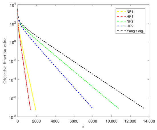
Figure 1. The objective function value versus the iteration number.

From Table 1 and Figure 1, we know that the inertial perturbation can improve the convergence of the algorithms and that the algorithms with Armijo-line search or self-adaptive step size perform better than Yang’s algorithm [3].

We also measure the restoration accuracy by means of the mean squared error, i.e., MSE $=(1/k)\parallel x^{\ast }-x^k\parallel$, where $x^{\ast }$ is an estimated signal of x. Figure 2 shows a comparison of the accuracy of the recovered signals when $m=1440,n=6144,p=180$. Given the same number of iterations, the recovered signals generated by algorithms in this paper outperform the one generated by Yang’s algorithm; NP1 needs more CPU time and presents lower accuracy; algorithms with self-adaptive step size perform better than the algorithms with step size determined by Armijo-line search in CPU time and imposing inertial perturbation accelerates the convergence rate and accuracy of signal recovery.

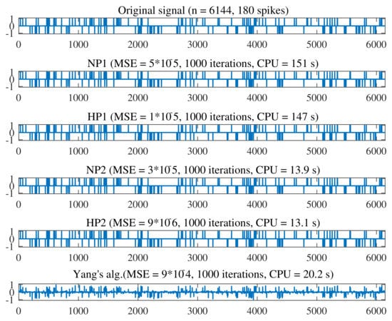
Figure 2. Comparison of signal processing.

5.2. Three MSSFP Problems

Example 1

([5]). Take ${\mathcal{H}}_1={\mathcal{H}}_2={\mathbf{R}}^3$, $r=t=2$, ${\beta }_1={\beta }_2=\frac{1}{2}$ and ${\alpha }_k=\gamma l^{m_k}$ for all $k\ge 1$, $\gamma =1,l=\frac{1}{2}$, $\mu =\frac{1}{2}$, ${\theta }_k=\frac{1}{4}$, ${\rho }_k=0.1$. Define

$$\begin{array}{ccc}\hfill C_1& =& \left\{x={(x_1,x_2,x_3)}^T\in {\mathbf{R}}^{\mathbf{3}}\mid x_1+x_2^2+2x_3\le 0\right\},\hfill \\ \hfill C_2& =& \left\{x={(x_1,x_2,x_3)}^T\in {\mathbf{R}}^{\mathbf{3}}\mid \frac{x_1^2}{16}+\frac{x_2^2}{9}+\frac{x_3^2}{4}-1\le 0\right\},\hfill \\ \hfill Q_1& =& \left\{x={(x_1,x_2,x_3)}^T\in {\mathbf{R}}^{\mathbf{3}}\mid x_1^2+x_2-x_3\le 0\right\},\hfill \\ \hfill Q_2& =& \left\{x={(x_1,x_2,x_3)}^T\in {\mathbf{R}}^{\mathbf{3}}\mid \frac{x_1^2}{4}+\frac{x_2^2}{4}+\frac{x_3^2}{9}-1\le 0\right\},\hfill \end{array}$$

and

$$\begin{array}{c}A=\left(\begin{array}{ccc}2& -1& 3\\ 4& 2& 5\\ 2& 0& 2\end{array}\right).\end{array}$$

The underlying MSSFP is to find $x^{\ast }\in C_1\bigcap C_2$ such that $A{x}^{\ast }\in Q_1\bigcap Q_2$.

We use inertial perturbation to accelerate the convergence of the algorithm. For the convenience of comparison, the initial values of the two inertial algorithms are set to be the same. Let $x^0=x^1$. We use $E_k=\parallel x^{k+1}-x^k\parallel /\parallel x^k\parallel$ to measure the error of the k-th iterate. If $E_k<{10}^{-5}$, then the iteration process stops. We compare our proposed iteration methods HP1, HP2 with NP1, NP2 and Liu and Tang’s Algorithm 2 in [29]. Algorithm 2 is of the form $x^{k+1}=U_{\left[k\right]}(x^k-{\alpha }_k{\sum }_{j=1}^r{\beta }_j{A}^{\ast }(I-T_j)Ax)$, ${\alpha }_k\in (0,\frac{2}{{\parallel A\parallel }^2})$. We take $U_{\left[k\right]}=P_{C_{\left[k\right]}^k}$, $T_j=P_{Q_j^k}$ and ${\alpha }_k=0.2\ast \frac{1}{{\parallel A\parallel }^2}$, and the algorithm is referred to as LT alg.

The convergence results and the CPU time of the five algorithms are shown in Table 2 and Figure 3. The errors are shown in Figure 4.

Table 2. Numerical results of five algorithms for Example 1.

Choice		NP1	HP1	NP2	HP2	LT Alg.
1. $x^0={(0.1,0.1,0.1)}^T$	No. of Iter	60	43	219	162	420
	cpu(time)	0.0511	0.0450	0.0362	0.0347	0.0879
2. $x^0={(-0.4,0.555,0.888)}^T$	No. of Iter	139	85	195	143	178
	cpu(time)	0.0669	0.0509	0.0342	0.0318	0.0552
3. $x^0={(1,2,3)}^T$	No. of Iter	142	89	195	141	178
	cpu(time)	0.0694	0.0490	0.0352	0.0339	0.0551
4. $x^0={(0.123,0.745,0.789)}^T$	No. of Iter	149	85	108	77	526
	cpu(time)	0.0590	0.0448	0.0295	0.0268	0.1018

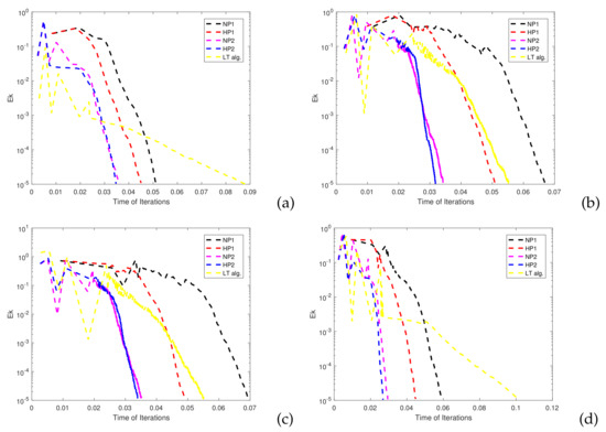
Figure 3. Comparison of CPU times of the algorithms in Example 1: (a) Comparison for choice 1. (b) Comparison for choice 2. (c) Comparison for choice 3. (d) Comparison for choice 4.

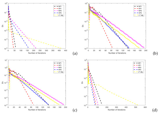
Figure 4. Comparison of iterations of the algorithms in Example 1: (a) Comparison for choice 1. (b) Comparison for choice 2. (c) Comparison for choice 3. (d) Comparison for choice 4.

The results show that (80) (HP2) outperforms (77) (HP1) for certain initial values. The main reason may be that the self-adaptive step size is more efficient than the one determined by the Armijo-line search. Comparison results of five algorithms and the convergence behavior show that in most cases, the convergence rate of the algorithm can be improved by adding an appropriate perturbation.

Example 2.

Take ${\mathcal{H}}_1={\mathbf{R}}^n$, ${\mathcal{H}}_2={\mathbf{R}}^m$, $A={\left(a_{ij}\right)}_{m\times n}$ with $a_{ij}\in (0,1)$ generated randomly, $C_i=\{x\in {\mathbf{R}}^n\mid \parallel x-d_i{\parallel }_2^2\le r_i^2\},i=1,2,\cdots ,t$, $Q_j=\{y\in {\mathbf{R}}^m\mid \parallel y-l_j{\parallel }_1^2\le h_j^2\},j=1,2,\cdots ,r$, where $d_i\in [{\mathbf{e}}_0,10{\mathbf{e}}_1]$, $r_i\in [40,60]$, $l_j\in [{\mathbf{e}}_0,{\mathbf{e}}_1]$, $h_j\in [10,20]$ are all generated randomly. Set ${\beta }_1={\beta }_2=\cdots ={\beta }_r=\frac{1}{r}$ and ${\alpha }_k=\gamma l^{m_k}$ for all $k\ge 1$, $\gamma =1,l=\frac{1}{2}$, $\mu =\frac{1}{2}$, ${\theta }_k=\frac{1}{4}$, ${\rho }_k=0.001$.

We consider using inertial perturbation to accelerate the convergence of the algorithm. If $E_k=\parallel x^{k+1}-x^k\parallel /\parallel x^k\parallel <{10}^{-4}$, then the iteration process stops. Let $x^0=x^1$. We choose arbitrarily three different initial points and consider iterative steps of the four algorithms with $m,n,r,t$ being different values. See Table 3 for details.

Table 3. Numerical results of the algorithms with and without perturbation for Example 2.

Initial Point		NP1	HP1	NP2	HP2
$r=t=10,m=15,n=20$
$x^0=x^1=2\ast e_1$	No. of Iter	49	36	1281	999
	cpu(time)	0.1031	0.0669	0.1480	1494
$x^0=x^1=50\ast e_1$	No. of Iter	187	121	2297	1669
	cpu(time)	0.2485	0.1536	0.2887	0.1868
$x^0=x^1=100\ast rand(n,1)$	No. of Iter	312	225	2357	1811
	cpu(time)	0.4202	0.2908	0.2830	0.2159
$r=t=10,m=n=40$
$x^0=x^1=2\ast e_1$	No. of Iter	89	66	956	732
	cpu(time)	0.3140	0.1777	0.1534	0.1318
$x^0=x^1=50\ast e_1$	No. of Iter	1710	1583	1301	1061
	cpu(time)	4.0390	4.0357	1860	0.1555
$x^0=x^1=100\ast rand(n,1)$	No. of Iter	1674	1658	1487	1219
	cpu(time)	4.6581	3.7752	0.2065	0.1762
$r=t=30,m=n=40$
$x^0=x^1=2\ast e_1$	No. of Iter	136	103	985	753
	cpu(time)	0.6912	0.5174	0.3312	0.2515
$x^0=x^1=50\ast e_1$	No. of Iter	1612	1411	1258	968
	cpu(time)	12.3437	11.7164	0.3991	0.3127
$x^0=x^1=100\ast rand(n,1)$	No. of Iter	1541	1133	1643	1012
	cpu(time)	11.8273	7.4646	1.0363	0.2965

In this example, we found that the algorithm with Armijo-line search needs fewer iteration steps in relatively low-dimensional spaces. In the case of high-dimensional spaces, the algorithm with self-adaptive step size outperforms in time. Generally, the convergence is improved by inertial perturbations for both algorithms in our paper.

Example 3

([30]). Take ${\mathcal{H}}_1={\mathbf{R}}^n$, ${\mathcal{H}}_2={\mathbf{R}}^m$, $A={\left(a_{ij}\right)}_{m\times n}$ with $a_{ij}\in (0,1)$ generated randomly, $C_i=\{x\in {\mathbf{R}}^n\mid \parallel x-d_i{\parallel }_2^2\le r_i^2\},i=1,2,\cdots ,t$, $Q_j=\{y\in {\mathbf{R}}^m\mid y^T{B}_{j}y+b_{j}y+c_j\le 0\},j=1,2,\cdots ,r$, where $d_i\in (6{\mathbf{e}}_0,16{\mathbf{e}}_1)$, $r_i\in (100,120)$, $b_j\in (-30{\mathbf{e}}_1,-20{\mathbf{e}}_1)$, $c_j\in (-50,-60)$, and all elements of the matrix $B_j$ are all generated randomly in the interval (2,10). Set ${\beta }_1={\beta }_2=\cdots ={\beta }_r=\frac{1}{r}$ and ${\alpha }_k=\gamma l^{m_k}$ for all $k\ge 1$, $\gamma =1,l=\frac{1}{2}$, $\mu =\frac{1}{2}$, ${\theta }_k=\frac{1}{4}$, ${\rho }_k=0.1$.

We consider using inertial perturbation to accelerate the convergence of the algorithm. The stopping criterion is defined by $E_k=\frac{1}{2}{\sum }_{i=1}^t\parallel x^k-P_{C_i^k}{x}^k{\parallel }^2+\frac{1}{2}{\sum }_{j=1}^r{\parallel A{x}^k-P_{Q_j^k}A{x}^k\parallel }^2<{10}^{-4}$. Let $x^0=x^1$. The details are shown in Table 4.

Table 4. Results of Armijo-line search and self-adaptive algorithms for Example 3.

Initial Point		NP1	HP1	NP2	HP2
$r=t=10,m=n=20$
$x^0=x^1=e_1$	No. of Iter	477	357	2268	1700
	cpu(time)	1.2453	0.9267	1.0516	0.8038
$x^0=x^1=50\ast e_1$	No. of Iter	757	564	3291	2470
	cpu(time)	1.6205	1.2805	1.5623	1.1023
$x^0=x^1=100\ast rand(n,1)$	No. of Iter	996	737	4323	3231
	cpu(time)	1.9087	1.4396	1.9696	1.4493
$r=t=20,m=40,n=50$
$x^0=x^1=e_1$	No. of Iter	1256	941	5336	4001
	cpu(time)	12.1310	4.0061	5.9165	4.0919
$x^0=x^1=50\ast e_1$	No. of Iter	1492	1105	6917	5221
	cpu(time)	12.6430	8.2382	12.9631	9.4880
$x^0=x^1=100\ast rand(n,1)$	No. of Iter	2101	1835	9936	9226
	cpu(time)	16.4070	13.2868	14.9611	12.8079
$r=t=40,m=n=60$
$x^0=x^1=e_1$	No. of Iter	1758	1317	8328	6245
	cpu(time)	48.2570	38.0668	30.6759	23.4267
$x^0=x^1=50\ast e_1$	No. of Iter	2503	1777	12,905	8677
	cpu(time)	59.2127	44.7915	49.5823	32.6868
$x^0=x^1=100\ast rand(n,1)$	No. of Iter	2274	1474	18,781	13,952
	cpu(time)	58.2569	38.1917	72.6622	54.9814

We can see from Table 4 that the convergence rate is improved by inertial perturbations for both algorithms. In most cases, the algorithm with step size determined by Armijo-line search outperforms the one with self-adaptive step size in the number of iterations, whereas the latter outperforms the former in CPU time.

6. Conclusions

In this paper, for the MSSFP, we present two relaxed CQ algorithms with different kinds of self-adaptive step size and discuss their bounded perturbation resilience. Treating appropriate inertial terms as bounded perturbations, we construct the inertial acceleration versions of the corresponding algorithms. For the real-life LASSO problem and three experimental examples, we numerically compare the performance with or without inertial perturbation of the algorithms and also compare the performance of the proposed algorithms with Yang’s algorithm [3], and Liu and Tang’s algorithm [29]. The results show the efficiency of the proposed algorithms and the validity of the inertial perturbation.

References

- Byrne, C. Iterative oblique projection onto convex sets and the split feasibility problem. Inverse Probl. 2002, 18, 441–453. [Google Scholar] [CrossRef]
- Byrne, C. A unified treatment of some iterative algorithms in signal processing and image reconstruction. Inverse Probl. 2004, 20, 103–120. [Google Scholar] [CrossRef]
- Yang, Q.Z. The relaxed CQ algorithm solving the split feasibility problem. Inverse Probl. 2004, 20, 1261–1266. [Google Scholar] [CrossRef]
- Censor, Y.; Elfving, T.; Kopf, N.; Bortfeld, T. The multiple-sets spilt feasibility problem and its applications for inverse problems. Inverse Probl. 2005, 21, 2071–2084. [Google Scholar] [CrossRef]
- He, S.N.; Zhao, Z.Y.; Luo, B. A relaxed self-adaptive CQ algorithm for the multiple-sets split feasibility problem. Optimization 2015, 64, 1907–1918. [Google Scholar] [CrossRef]
- Yang, Q.Z. On variable-step relaxed projection algorithm for variational inequalities. J. Math. Anal. Appl. 2005, 302, 166–179. [Google Scholar] [CrossRef]
- López, G.; Martín-Márquez, V.; Wang, F.H.; Xu, H.K. Solving the split feasibility problem without prior knowledge of matrix norms. Inverse Probl. 2012, 28, 374–389. [Google Scholar] [CrossRef]
- Gibali, A.; Liu, L.W.; Tang, Y.C. Note on the the modified relaxation CQ algorithm for the split feasibility problem. Optim. Lett. 2018, 12, 817–830. [Google Scholar] [CrossRef]
- Chen, Y.; Guo, Y.; Yu, Y.; Chen, R. Self-adaptive and relaxed self-adaptive projection methods for solving the multiple-set split feasibility problem. Abstr. Appl. Anal. 2012, 2012, 958040. [Google Scholar] [CrossRef]
- Xu, H.K. Iterative methods for the split feasibility problem in infinite-dimensional Hilbert spaces. Inverse Probl. 2010, 26, 105018. [Google Scholar] [CrossRef]
- Xu, H.K. A variable Krasnosel’skii-Mann algorithm and the multiple-set split feasibility problem. Inverse Probl. 2006, 22, 2021–2034. [Google Scholar] [CrossRef]
- Yao, Y.H.; Postolache, M.; Liou, Y.C. Strong convergence of a self-adaptive method for the split feasibility problem. Fixed Point Theory Appl. 2013, 2013, 201. [Google Scholar] [CrossRef]
- Guo, Y.N.; Cui, W.; Guo, Y.S. Perturbation resilience of proximal gradient algorithm for composite objectives. J. Nonlinear Sci. Appl. 2017, 10, 5566–5575. [Google Scholar] [CrossRef][Green Version]
- Guo, Y.N.; Cui, W. Strong convergence and bounded perturbation resilience of a modified proximal gradient algorithm. J. Inequalities Appl. 2018, 2018, 103. [Google Scholar] [CrossRef] [PubMed]
- Pakkaranang, N.; Kumam, P.; Berinde, V.; Suleiman, Y.I. Superiorization methodology and perturbation resilience of inertial proximal gradient algorithm with application to signal recovery. J. Supercomput. 2020, 76, 9456–9477. [Google Scholar] [CrossRef]
- Jin, W.M.; Censor, Y.; Jiang, M. Bounded perturbation resilience of projected scaled gradient methods. Comput. Optim. Appl. 2016, 63, 365–392. [Google Scholar] [CrossRef]
- Xu, H.K. Bound perturbation resilience and superiorization techniques for the projected scaled gradient method. Inverse Probl. 2017, 33, 044008. [Google Scholar] [CrossRef]
- Dong, Q.L.; Gibali, A.; Jiang, D.; Tang, Y. Bounded perturbation resilience of extragradient-type methods and their applications. J. Inequalities Appl. 2017, 2017, 280. [Google Scholar] [CrossRef] [PubMed]
- Duan, P.C.; Zheng, X.B. Bounded perturbation resilience of generalized viscosity iterative algorithm for split variational inclusion problem. Appl. Set-Valued Anal. Optim. 2020, 2, 49–61. [Google Scholar]
- Censor, Y.; Zaslavski, A.J. Convergence and perturbation resilience of dynamic string-averaging projection methods. Comput. Optim. Appl. 2013, 54, 65–76. [Google Scholar] [CrossRef]
- Kaewyong, N.; Sitthithakerngkiet, K. A self-adaptive algorithm for the common solution of the split minimization problem and the fixed point problem. Axioms 2021, 10, 109. [Google Scholar] [CrossRef]
- Shehu, Y.; Dong, Q.L.; Liu, L.L. Global and linear convergence of alternated inertial methods for split feasibility problems. R. Acad. Sci. 2021, 115, 53. [Google Scholar]
- Li, H.Y.; Wu, Y.L.; Wang, F.H. New inertial relaxed CQ algorithms for solving split feasibility problems in Hilbert spaces. J. Math. 2021, 2021, 6624509. [Google Scholar] [CrossRef]
- Bauschke, H.H.; Combettes, P.L. Convex Analysis and Monotone Operator Theory in Hilbert Space; Springer: London, UK, 2011. [Google Scholar]
- Bauschke, H.H.; Combettes, P.L. A weak-to-strong convergence principle for Fejér-monntone methods in Hilbert spaces. Math. Oper. Res. 2001, 26, 248–264. [Google Scholar] [CrossRef]
- Wen, M.; Peng, J.G.; Tang, Y.C. A cyclic and simultaneous iterative method for solving the multiple-sets split feasibility problem. J. Optim. Theory Appl. 2015, 166, 844–860. [Google Scholar] [CrossRef]
- Sun, J.; Dang, Y.Z.; Xu, H.L. Inertial accelerated algorithms for solving a split feasibility problem. J. Ind. Manag. Optim. 2017, 13, 1383–1394. [Google Scholar]
- Tang, Y.C.; Zhu, C.X.; Yu, H. Iterative methods for solving the multiple-sets split feasibility problem with splitting self-adaptive step size. Fixed Point Theory Appl. 2015, 2015, 178. [Google Scholar] [CrossRef]
- Liu, L.W.; Tang, Y.C. Several iterative algorithms for solving the split common fixed point problem of directed operators with applications. Optim. A J. Math. Program. Oper. Res. 2016, 65, 53–65. [Google Scholar]
- Zhao, J.L.; Yang, Q.Z. Self-adaptive projection methods for the multiple-sets split feasibility problem. Inverse Probl. 2011, 27, 035009. [Google Scholar] [CrossRef]
Publisher’s Note: MDPI stays neutral with regard to jurisdictional claims in published maps and institutional affiliations. |
© 2021 by the authors. Licensee MDPI, Basel, Switzerland. This article is an open access article distributed under the terms and conditions of the Creative Commons Attribution (CC BY) license (https://creativecommons.org/licenses/by/4.0/).