Hypersingular Integral Equations of Prandtl’s Type: Theory, Numerical Methods, and Applications

Abstract

In this paper, we propose and justify a spline-collocation method with first-order splines for approximate solution of nonlinear hypersingular integral equations of Prandtl’s type. We obtained the estimates of the convergence rate and the method error. The constructed computational scheme includes a continuous method for solving nonlinear operator equations, which is stable for perturbations of the coefficients and the right-hand sides of equations.

1. Introduction

Singular and hypersingular integral equations are widely used in aerodynamics. Two-dimensional flows in aerodynamics are described by the thin-wing equation

$${\int }_{-l}^l\frac{x\left(\tau \right)d\tau }{\tau -t}=f\left(t\right)$$

(1)

and the Prandlt integrodifferential equation

$$\frac{x\left(t\right)}{B\left(t\right)}+{\int }_{-1}^1\frac{x^{\prime }\left(\tau \right)}{\tau -t}d\tau =f\left(t\right).$$

(2)

Active research into two-dimensional aerodynamics problems started in the 1930s. The main results were obtained by V. V. Golubev [1], T. von Karman and Y. M.Burgers [2], H. Schmidt [3] and K. Schröder [4,5].

The theory of two-dimensional equations in aerodynamics was further developed by H. Küsner and Schwarz [6], L. G. Magnarange [7], I. N. Vekua [8], and Y. Weissinger [9].

The hypersingular integral equation

$${\int \int }_G\frac{x({\tau }_1,{\tau }_2)}{{({\tau }_2-t_2)}^2}\left(1+\frac{{\tau }_1-t_1}{\sqrt{{({\tau }_1-t_1)}^2+{({\tau }_2-t_2)}^2}}\right)d{\tau }_{1}d{\tau }_2=f(t_1,t_2),$$

(3)

where $f(t_1,t_2)\in H$, H stands for a Hölder class, plays an important role in the theory of a finite wing in three dimensions [10,11].

The two-dimensional integrodifferential Equation [12] should also be regarded as Prandtl’s type equations

$${\int }_{-a}^a{\int }_{-l}^l{x}_{{\tau }_2}^{\prime }({\tau }_1,{\tau }_2)\frac{t_1+{\tau }_1+\sqrt{a^2+(t_2-{\tau }_2)}}{(t_1-{\tau }_1)(t_2-{\tau }_2)}d{\tau }_{1}d{\tau }_2=f(t_1,t_2),$$

(4)

where $-a<t_1<a,-l<t_2<l$, and function $f(t_1,t_2)\in H$ in $[-a,a;-l,l]$.

Despite their history of more than a century, active investigation of two-dimensional aerodynamics problems using the methods of singular integral equations—including Prandtl’s type equation—continues. We should note here the works by S. M. Belotserkovsky and I. K. Lifanov [10], Y. Blackwell and G. Pounds [13], S. R. Bland et al. [14], Y A. Fromme and M. A. Golberg [15], M. A. Golberg [16], A. Kalandia [17], E. Kraft and C. Lo [18], E. G. Ladopoulos [19], I. K. Lifanov [20], M. Mokry [21], W. F. Moss [22], D. Y. Salmond [23], and M. Sheshko [24].

Along with equations on a segment, the Prandtl-type equations on a real half-line

$$x\left(t\right)-\frac{a\left(t\right)}{\pi }{\int }_0^{\infty }\frac{x^{\prime }\left(\tau \right)}{\tau -t}d\tau =f\left(t\right)$$

and on the real axis

$$x\left(t\right)-\frac{a\left(t\right)}{\pi }{\int }_{-\infty }^{\infty }\frac{x^{\prime }\left(\tau \right)}{\tau -t}d\tau =f\left(t\right)$$

have also been investigated.

The classical Prandtl equation [25] has the form

$$\frac{x\left(t\right)}{B\left(t\right)}-\frac{1}{\pi }{\int }_{-1}^1\frac{x^{\prime }\left(\tau \right)}{\tau -t}d\tau =f\left(t\right),-1<t<1.$$

(5)

Here $B\left(t\right),f\left(t\right)\in C[-1,1]$ are known functions, and $x\left(t\right)$ is a desired function. Boundary conditions are assigned to the Equation (5)

$$x(-1)=\alpha ,x\left(1\right)=\beta .$$

(6)

In wing theory [1], one assumes $\alpha =0,\beta =0,$ and in contact problems [26], $\alpha =0,\beta =1$.

A large number of manuscripts are devoted to this equation. The results obtained in the 1920–1940s are summarized by V. V. Golubev [1]. One also can find an extensive bibliography in [1]. Recent results can be found in [17,26].

Along with Equation (5), the equations of the form

$$a\left(t\right)x\left(t\right)+\frac{b\left(t\right)}{\pi }\underset{a}{\overset{b}{\int }}\frac{x^{\prime }\left(\tau \right)}{\tau -t}d\tau =f\left(t\right),a<t<b,$$

with various limits of “a” and “b”, which are studied for various boundary and initial conditions, are called Prandtl type equations.

The Prandtl equation of the form

$$x\left(t\right)-\frac{a\left(t\right)}{\pi }{\int }_{-\infty }^{\infty }\frac{x^{\prime }\left(\tau \right)d\tau }{\tau -t}=f\left(t\right),t\in R\backslash \left\{0\right\},$$

(7)

with discontinuous function $a\left(t\right)$ is studied [27] in the theory of elasticity for bodies with thin layers and in hydromechanics.

In the theory of elasticity, we also consider the equation

$$a\left(t\right)x\left(t\right)+\frac{\lambda }{\pi }{\int }_0^{\infty }\frac{x^{\prime }\left(\tau \right)}{\tau -t}d\tau =f\left(t\right),t\in R_{+},\lambda =const>0,$$

(8)

with the boundary condition

$$x\left(0\right)=c_0\ne 0.$$

(9)

A special case of (5) appears to be a homogeneous equation

$$2\lambda \phi =A\phi ,\left(A\phi \right)\left(t\right)={\int }_0^1\frac{{\phi }^{\prime }\left(\tau \right)d\tau }{t-\tau }.$$

(10)

It can be found in numerous applications (aerodynamics, a plane problem of elasticity theory, and automatic control). A lot of works are devoted to this study. The main bibliography of the 1920s and 1930s is given in the first edition of the book by N. I. Muskhelishvili [28] and in [29]).

Using the change in variables $t=(1+\xi )/2,\tau =(1+\eta )/2$, one reduces the Equation (10) to the standard form [30]

$$\lambda \phi \left(t\right)={\int }_{-1}^1\frac{{\phi }^{\prime }\left(\tau \right)d\tau }{t-\tau }.$$

(11)

For certain Prandtl-type equations, there are known solutions in analytical form. For a homogeneous equation on a half-line, the exact analytical solution of Prandtl’s equation was obtained in [31] using Mellin and Laplace transforms. The analytical solution of Prandtl’s inhomogeneous equation on a half-line has been obtained by transforming the equation into a Riemann boundary problem employing the Fourier transform [32]. The Prandtl equation on a closed segment can be solved by three analytical methods: (a) analytical continuation of an integral to the complex plane [8]; (b) the Kellermann–Vekua regularization [26,33]; (c) reducing the problem to an infinite system of algebraic equations by expanding the desired solution in terms of Chebyshev, Lagrange, or Jacobi orthogonal polynomials [26,33].

In the works known to the authors, linear singular integro-differential equations modeling the equation of the wing in a linearized formulation have been investigated. To derive the Prandtl equation, a number of linearizations have been provided in [1]. Repeating without simplification the arguments in [1], we arrive at the nonlinear integro-differential wing equation, which is a special case of the hypersingular integral equations with singularities of the second order discussed below.

As noted above, for the wing theory problems, the Prandtl equation is studied with the boundary conditions $x(-1)=x\left(1\right)=0.$ Furthermore, it requires $x^{\prime }\left(t\right)\in H^{*}$. As $x(-1)=x\left(1\right)=0$, from $x^{\prime }\left(t\right)\in H^{*}$, it follows that for any finite values at the nodes $x(-1),x\left(1\right)$, a solution of the Equation (5) is a continuous and bounded function in $[-1,1]$.

Recall [34] that $\psi \left(x\right)\in H^{*}$ if it satisfies the Holder condition in $[-1+{\epsilon }_1,1-{\epsilon }_2],$${\epsilon }_1>0,{\epsilon }_2>0.$ It yields an integrable singularity of the form

$$\psi \left(t\right)=\frac{{\psi }_0\left(t\right)}{{(1-t^2)}^{\gamma }},0\le \gamma <1,$$

near the points $\pm 1.$ The function ${\psi }_0\left(t\right)$ satisfies the Holder condition in $[-1,1].$

Such a formulation leads to more restrictive class of problems that are modeled by the Prandtl equation.

In this paper, we study Prandtl-type hypersingular integral equations with unbounded solutions at the endpoints of the segment $[-1,1].$ We turn to the Prandtl-type hypersingular integral equations for the following reasons. It is impossible to find solution in the class of functions $x\left(t\right)={(1-t^2)}^{\gamma }\phi \left(t\right),-1<\gamma <0$ for Prandtl’s equation in the standard form

$$\frac{x\left(t\right)}{B\left(t\right)}+{\int }_{-1}^1\frac{x^{\prime }\left(\tau \right)}{\tau -t}d\tau =f\left(t\right),$$

where the integral is considered in the sense of Cauchy. The derivative $x^{\prime }\left(t\right)$ has singularities ${(1-t^2)}^{-1-\gamma }$ and is non-integrable in the sense of Cauchy’s principal value. Prandtl-type hypersingular integral equations admit such classes of solutions. When modeling filtering problems with the hypersingular integral equation

$$\frac{x\left(t\right)}{B\left(t\right)}+{\int }_{-1}^1\frac{x\left(\tau \right)}{{(\tau -t)}^2}d\tau =f\left(t\right),$$

where the hypersingular integral is defined by the formula

$${\int }_{-1}^1\frac{x\left(\tau \right)}{{(\tau -t)}^2}d\tau =\frac{d}{dt}{\int }_{-1}^1\frac{x\left(\tau \right)}{\tau -t}d\tau ,$$

such solutions can be considered.

A number of problems in the theory of composite materials are modeled [35,36] by nonlinear hypersingular integral equations of the Prandtl form

$${\int }_{-1}^1\frac{x\left(\tau \right)}{{(\tau -t)}^2}d\tau +a\left(x\left(t\right)\right)=f\left(t\right).$$

(12)

Turning to hypersingular integral equations of the Prandtl form allows us to extend a class of applied problems by using much broader classes of functions.

Extensive bibliography is devoted to the study of the Equations (5) and (11). In addition to the works mentioned above, the uniqueness of the Equation (5) solution in various functional classes has been investigated in [24].

It is shown that for $\sqrt{1-t^2}<\left|B\left(t\right)\right|$, the boundary problem (5) and (6) (for $\alpha =\beta =0$) has the unique solution in the class of functions $x^{\prime }\left(t\right)\in H^{*}$.

The study of existence and uniqueness of the solutions of nonlinear singular integro-differential equations (including the Prandtl equation) is given in [37].

The Equation (11) has been investigated in [30,38].

Despite numerous efforts, an analytical form of Prandtl’s equation solution can be found only in special cases. The progress in applications of Prandtl’s equation is conditioned by the development of numerical methods. The broad literature on this subject is given in [17,26,32,35,39,40,41]. There, the collocation method and the method of moments have been used. Recently, homotopy methods have been employed to solve Prandtl’s equations [39,42].

Let us review these methods more thoroughly. One of the first approximate methods for solving the Equation (5) was Multhopp’s method [43]. Its complete justification based on the constructive function theory is given in [17]. The articles [24,44] are devoted to modifications of the Multhopp method. The approximation methods constructed there converge under conditions $\sqrt{1-t^2}<\left|B\left(t\right)\right|$ to the exact solution of the boundary problem (5), $x(-1)=x\left(1\right)=0$ with rate

$$\parallel x\left(t\right)-x_n{\left(t\right)\parallel }_C=O\left(\frac{lnn}{\sqrt{n}}\right),$$

where $x_n\left(t\right)$ is an approximate solution and n is a number of functionals studied when constructing $x_n\left(t\right)$. The methods are based on the transformation of the Equation (5) with boundary conditions $x(-1)=x\left(1\right)=0$ to an equivalent Fredholm equation with a logarithmic singularity. The transformation is based on the inversion formula for a singular integro-differential operator [30]

$$\psi \left(t\right)=-\frac{1}{\pi }\underset{-1}{\overset{1}{\int }}\frac{{\phi }^{\prime }\left(\tau \right)d\tau }{\tau -t}:$$

$$\phi \left(t\right)=\underset{-1}{\overset{1}{\int }}h(\tau ,t)\psi \left(\tau \right)d\tau +c_{1}arcsint+c_2,$$

where $h(\tau ,t)=\frac{1}{2{\pi }^2}ln\frac{1-\tau t+\sqrt{(1-{\tau }^2)(1-t^2)}}{1-\tau t-\sqrt{(1-{\tau }^2)(1-t^2)}}$.

As described above, the boundary value problem (5), $x(-1)=x\left(1\right)=0$ can be represented by a hypersingular integral equation

$$\underset{-1}{\overset{1}{\int }}\frac{x\left(\tau \right)d\tau }{{(\tau -t)}^2}+a\left(t\right)x\left(t\right)=f\left(t\right).$$

(13)

The Equation (13) is a special case of a more general equation

$$a\left(t\right)x\left(t\right)+b\left(t\right)\underset{-1}{\overset{1}{\int }}\frac{x\left(\tau \right)d\tau }{{(\tau -t)}^2}+\underset{-1}{\overset{1}{\int }}h(t,\tau )x\left(\tau \right)d\tau =f\left(t\right),$$

(14)

an approximate solution of which has been studied in multiple works; a review can be found in [45]. Among the more recent works that were published after 2019, we would like to mention [46,47,48].

The unique solvability of the spline-collocation method with splines of zero order has been justified in [49]. In the same paper, a spline-collocation method with splines of the first order was constructed, and its unique solvability was justified. Assuming that the solution belongs to the set of functions $W^2(M;[-1,1])$, the convergence of the method to the exact solution of the original equation has been justified for linear equations.

The problem of convergence of approximate solution to exact solution remains unanswered for nonlinear hypersingular integral equations. In this paper, we cover it for certain classes of equations.

In this paper, we also construct and justify spline-collocation methods with first-order splines for approximate solutions of nonlinear hypersingular integral equations of the first kind, including the Prandtl equation.

We justified the unique solvability and the convergence of the presented methods with first-order splines.

2. Continuous Method and Its Convergence Properties

The method we employ in the next section for solving hypersingular integral equations is based on the continuous method for the solution of nonlinear operator equations, introduced in [50]. One of the further advantages of the method we propose here is that—in contrast to Newton–Kantorovich type of methods—the method does not require continuous invertibility of the Frechet derivative and still demonstrate convergence in the case when the Frechet derivative is degenerate.

We use the following notation:

$B(a,r)=\{z\in B:\parallel z-a\parallel \le r\}$, $S(a,r)=\{z\in B:\parallel z-a\parallel =r\}$, $Re\left(K\right)=\Re \left(K\right)=(K+K^{*})/2$, $\mathsf{\Lambda }\left(K\right)=\underset{h\downarrow 0}{lim}(\parallel I+hK\parallel -1)h^{-1}$. Here, B is a Banach space, $a\in B$, K is a linear and bounded operator on B, $\mathsf{\Lambda }\left(K\right)$ is the logarithmic norm [51] of the operator K, $K^{*}$ is the conjugate operator to K, and I stands for the identity operator.

The logarithmic norm is known for operators in the most frequently used spaces.

Let $A=\left\{a_{ij}\right\}$, $i,j=1,2,\dots ,n$, be a real matrix.

In the n-dimensional space $R_n$ of vectors $x=(x_1,\dots ,x_n)$. the following norms are used the most:

${\parallel x\parallel }_1={\displaystyle \sum _{i=1}^n}\left|x_i\right|;$

${\parallel x\parallel }_2=\underset{1\le i\le n}{max}\left|x_i\right|;$

${\parallel x\parallel }_3={({\displaystyle \sum _{i=1}^n}{x}_i^2)}^{1/2}.$

Here are some expressions of the logarithmic norm of a matrix $A=\left(a_{ij}\right),$ due to the above norms of the vectors:

logarithmic norm ${\mathsf{\Lambda }}_1$

$${\mathsf{\Lambda }}_1\left(A\right)=\underset{1\le j\le n}{max}\left(a_{jj}+\sum _{i\ne j}\left|a_{ij}\right|\right);$$

logarithmic norm ${\mathsf{\Lambda }}_2$

$${\mathsf{\Lambda }}_2\left(A\right)=\underset{1\le i\le n}{max}\left(a_{ii}+\sum _{j\ne i}\left|a_{ij}\right|\right);$$

logarithmic norm ${\mathsf{\Lambda }}_3$

$${\mathsf{\Lambda }}_3\left(A\right)={\lambda }_{max}\left(\frac{A+A^{*}}{2}\right),$$

where $A^{*}$ is the conjugate matrix for $A.$

The logarithmic norm has the property that is very useful for numerical analysis.

Let $A,B$ be square matrices of order n with complex elements and $x=(x_1,\dots ,x_n)$, $y=(y_1,\dots ,y_n)$, $\xi =({\xi }_1,\dots ,{\xi }_n)$, and $\eta =({\eta }_1,\dots ,{\eta }_n)$ are n-dimensional vectors with complex components. Let us consider the following systems of algebraic equations: $Ax=\xi$ and $By=\eta$. The norm of a vector and its subordinate operator norm of the matrix are fixed; the logarithmic norm $\mathsf{\Lambda }\left(A\right)$ corresponds to the operator norm.

Theorem 1 

([52]). If $\mathsf{\Lambda }\left(A\right)<0$, then the matrix A is non-singular and $\parallel A^{-1}\parallel \le 1/\left|\mathsf{\Lambda }\left(A\right)\right|$.

Theorem 2 

([52]). Let $Ax=\xi$, $By=\eta$ and $\mathsf{\Lambda }\left(A\right)<0$, $\mathsf{\Lambda }\left(B\right)<0$. Then

$$\parallel x-y\parallel \le \frac{\parallel \xi -\eta \parallel }{\left|\mathsf{\Lambda }\right(B\left)\right|}+\frac{\parallel A-B\parallel }{\left|\mathsf{\Lambda }\right(A\left)\mathsf{\Lambda }\right(B\left)\right|}.$$

Let us consider the continuous method for solving nonlinear operator equations.

Consider a nonlinear operator equation

$$A\left(x\right)=0.$$

(15)

Here, A is a nonlinear operator that acts from a Banach space B into B. In the Banach space B, consider the Cauchy problem

$$\frac{dx\left(t\right)}{dt}=A\left(x\left(t\right)\right),$$

(16)

$$x\left(0\right)=x_0.$$

(17)

We assume that the nonlinear operator A has a continuous Frechet derivative and $A\left(0\right)=0$.

Let us present conditions for the global convergence of the solution of the Cauchy problem (16) and (17) to the solution of the Equation (15).

The following assertions have been proved in [50].

Theorem 3 

([50]). Let the Equation (15) have a solution $x^{*}$, and let inequality

$$\underset{t\to \infty }{lim}\frac{1}{t}\underset{0}{\overset{t}{\int }}\mathsf{\Lambda }\left(A^{\prime }\left(g\left(\tau \right)\right)\right)d\tau \le -\alpha ,\alpha >0,$$

(18)

be true on each differentiable curve $g\left(t\right)$ lying in the Banach space B. Then, the solution of the Cauchy problem (16) and (17) converges to the solution $x^{*}$ of the Equation (15) for any initial value $x_0\in B.$

It follows from inequality (18) that the Theorem 3 is also valid in cases when the logarithmic norm $\mathsf{\Lambda }\left(A^{\prime }\left(x\right)\right)$ can take zero or positive and bounded values at finitely n countably many points of the space B.

Theorem 4 

([50]). Let the Equation (15) have a solution $x^{*}$, and let the following conditions be satisfied on any differentiable curve $g\left(t\right)$ lying in the ball $B(x^{*},r)$:

1. The inequality

$$\underset{0}{\overset{t}{\int }}\mathsf{\Lambda }\left(A^{\prime }\left(g\left(\tau \right)\right)\right)d\tau \le 0$$

holds for all $t(t>0)$.

2. Inequality (18) is satisfied.

Then the solution of the Cauchy problem (16) and (17) converges to the solution $x^{*}$ of the Equation (15).

The proofs of Theorems are based on sufficient conditions for asymptotic stability of systems of nonlinear differential equations in Banach spaces [53,54].

3. Approximate Solution of the Nonlinear Prandtl Equation

Let us consider a Prandtl nonlinear hypersingular integral equation

$$a(t,x\left(t\right))+\underset{-1}{\overset{1}{\int }}\frac{x\left(\tau \right)d\tau }{{(\tau -t)}^2}=f\left(t\right),$$

(19)

where $a(t,x(t\left)\right)$ is a function continuous with respect to the first variable and continuously differentiable with respect to the second variable.

Let us construct a computational scheme for the approximate solution of the Equation (19) and justify it.

To solve the Equation (19), we suggest two computational schemes below.

3.1. First Computational Scheme

We now discuss the case where the right-hand side of the Equation (19) is bounded in the interval $[-1,1].$

Let $t_k=-1+(k/N),k=0,1,...,N,t_k=1-\left(\frac{2N-k}{N}\right),k=N+1,...,2N.$ Let ${\Delta }_k=[t_k,t_{k+1}),$$k=0,1,...,N-2,$ ${\Delta }_{2N-1}=[t_{2N-1},t_{2N}].$

An approximate solution of the Equation (19) we will seek as

$$x_N\left(t\right)=\sum _{k=0}^{2N}{\alpha }_k{\psi }_k\left(t\right)$$

(20)

with basis functions ${\psi }_k\left(t\right).$ For the nodes $t_k,$$k=1,\dots ,2N-1,$ the corresponding basis elements are determined by

$${\phi }_k\left(t\right)=\left\{\begin{array}{cc}0,\hfill & t_{k-1}\le t\le t_{k-1}+\frac{1}{N^2},\hfill \\ \frac{N^2}{N-2}(t-t_{k-1})-\frac{1}{N-2},\hfill & t_{k-1}+\frac{1}{N^2}\le t\le t_k-\frac{1}{N^2},\hfill \\ 1,\hfill & t_k-\frac{1}{N^2}\le t\le t_k+\frac{1}{N^2},\hfill \\ -\frac{N^2}{N-2}(t-t_{k+1})-\frac{1}{N-2},\hfill & t_k+\frac{1}{N^2}\le t\le t_{k+1}-\frac{1}{N^2},\hfill \\ 0,\hfill & t_{k+1}-\frac{1}{N^2}\le t\le t_{k+1},\hfill \\ 0,\hfill & t\in [-1,1]\backslash [t_{k-1},t_{k+1}].\hfill \end{array}\right.$$

(21)

For boundary nodes $t_k,$$k=0$ and $k=2N$, the corresponding basis elements are defined as

$${\phi }_0\left(t\right)=\left\{\begin{array}{cc}1,\hfill & -1\le t\le -1+\frac{1}{N^2},\hfill \\ -\frac{N^2}{N-2}(t-t_1)-\frac{1}{N-2},\hfill & -1+\frac{1}{N^2}\le t\le t_1-\frac{1}{N^2},\hfill \\ 0,\hfill & t_1-\frac{1}{N^2}\le t\le t_1,\hfill \\ 0,\hfill & [-1,1]\backslash [t_0,t_1];\hfill \end{array}\right.$$

(22)

and

$${\phi }_{2N}\left(t\right)=\left\{\begin{array}{cc}0,\hfill & -1\le t\le t_{N-1}+\frac{1}{N^2},\hfill \\ \frac{N^2}{N-2}(t-t_{N-1})-\frac{1}{N-2},\hfill & t_{N-1}+\frac{1}{N^2}\le t\le 1-\frac{1}{N^2},\hfill \\ 1,\hfill & 1-\frac{1}{N^2}\le t\le 1.\hfill \end{array}\right.$$

(23)

A spline-collocation method constructed by nodes $t_k$ has a form

$$\begin{array}{c}a(t_k,x\left(t_k\right))+{\displaystyle \sum _{l=0}^{2N}}{\alpha }_l\underset{-1}{\overset{1}{\int }}\frac{{\psi }_l\left(\tau \right)}{{(\tau -t_k)}^2}d\tau =f\left(t_k\right),k=0,1,..,2N.\hfill \end{array}$$

(24)

In some cases below, the following computational scheme is preferred,

$$\begin{array}{c}{\displaystyle a(t_k,x\left(t_k\right))+\sum _{l=0}^{2N}{}^{*}{\alpha }_l{\int }_{-1}^1\frac{{\psi }_l\left(\tau \right)}{{(\tau -t_k)}^2}d\tau =f\left(t_k\right),k=0,1,..,2N,}\hfill \end{array}$$

(25)

where $\sum {}^{*}$ means summation over $|l-k|\ne 1.$

Note that at the nodes $\pm 1$, the hypersingular integral is evaluated by the definition given in [55],

$${\int }_a^b\frac{\phi \left(\tau \right)d\tau }{{(\tau -a)}^2}=\underset{v\downarrow 0}{lim}\left[{\int }_{a+v}^b\frac{\phi \left(\tau \right)}{{(\tau -a)}^2}d\tau +\frac{\epsilon \left(v\right)}{v}+{\epsilon }_1\left(v\right)lnv\right],$$

where $\epsilon \left(v\right)$ is an arbitrary function with continuous derivatives near zero and ${\epsilon }_1\left(v\right)$ is an arbitrary function satisfying Dini–Lipschitz near zero. The functions $\epsilon \left(v\right)$ and ${\epsilon }_1\left(v\right)$ are chosen so that the limit exists.

To solve the system (24), we employ the continuous method for solving nonlinear operator equations.

Let

$$g_{kl}={\int }_{-1}^1\frac{{\psi }_l\left(\tau \right)}{{(\tau -t_k)}^2}d\tau .$$

A collocation method for the Equation (24) is written as

$$a(t_k,{\alpha }_k)+\sum _{l=0}^{2N}{\alpha }_l{g}_{kl}=f\left(t_k\right),k=0,1,..,2N.$$

(26)

The system of Equation (26) can be rewritten in the operator form

$$K_{2N}{x}_N\equiv P_{2N}\left[a(t,x_N\left(t\right))+\underset{-1}{\overset{1}{\int }}\frac{x_N\left(\tau \right)d\tau }{{(\tau -t)}^2}\right]=P_{2N}\left[f\left(t\right)\right],$$

(27)

where $P_{2N}\left[f\left(t\right)\right]$ denotes an operator of projecting the function $f\left(t\right)$ on $2N+1-$dimensional vector $(f\left(t_0\right),f\left(t_1\right),\dots ,f\left(t_{2N}\right)).$

A Frechet derivative for operator on the left-hand side of the Equation (24) on $x_0\left(t\right)$ has the form

$$a_2^{\prime }(t,x_0\left(t\right))x\left(t\right)+\underset{-1}{\overset{1}{\int }}\frac{x\left(\tau \right)d\tau }{{(\tau -t)}^2},$$

(28)

where $a_2^{\prime }(t,u)$ denotes a derivative with respect to the second variable.

The derivative of $K_{2N}$ on the element $\mathsf{\Gamma }=({\gamma }_0,{\gamma }_1,\dots ,{\gamma }_{2N})$ has a form of a matrix H with elements $H=\left\{h_{k,l}\right\},k,l=0,1,\dots ,2N$, where $h_{k,k}=a_2{}^{\prime }(t_k,{\gamma }_k)+\underset{-1}{\overset{1}{\int }}\frac{{\psi }_k\left(\tau \right)d\tau }{{(\tau -t_k)}^2},$

$k=0,1,\dots ,2N$, $h_{k,l}=\underset{-1}{\overset{1}{\int }}\frac{{\psi }_l\left(\tau \right)d\tau }{{(\tau -t_k)}^2},k,l=0,1,\dots ,2N$.

Below, we provide the proof of the unique solvability for computational scheme (24) based on an estimate of the logarithmic norm ${\mathsf{\Lambda }}_3\left(H\right)$ for the matrix H.

Let us estimate the logarithmic norm in the space $R_{2N+1}$ of $2N+1-$dimensional vectors $x=(x_0,x_1,..,x_{2N})$ with the norm $\parallel x\parallel =\underset{0\le i\le 2N}{max}\left|x_i\right|$.

Evaluate integrals $g_{kl},k,l=0,1,\dots ,2N$.

$$\underset{t_{k-1}}{\overset{t_{k+1}}{\int }}\frac{{\phi }_k\left(\tau \right)d\tau }{{(\tau -t_k)}^2}=-2N^2\frac{ln(N-1)}{N-2},$$

(29)

$$\underset{-1}{\overset{t_1}{\int }}\frac{{\phi }_0\left(\tau \right)d\tau }{{(\tau +1)}^2}=-N^2\frac{ln(N-1)}{N-2},$$

(30)

$$\underset{t_{2N-1}}{\overset{1}{\int }}\frac{{\phi }_{2N}\left(\tau \right)d\tau }{{(\tau -1)}^2}=-N^2\frac{ln(N-1)}{N-2},$$

(31)

$$\underset{-1}{\overset{1}{\int }}\left[\sum _{l=1}^{2N}{\phi }_l\left(\tau \right)\right]\frac{d\tau }{{(\tau +1)}^2}=\frac{N^2}{N-2}ln(N-1)-\frac{1}{2},$$

(32)

$$\underset{-1}{\overset{1}{\int }}\left[\sum _{l=0}^{2N-1}{\phi }_l\left(\tau \right)\right]\frac{d\tau }{{(\tau -1)}^2}=\frac{N^2}{N-2}ln(N-1)-\frac{1}{2},$$

(33)

$$\underset{-1}{\overset{1}{\int }}\left[\sum _{l=0}^{2N}{}^{\prime }{\phi }_l\left(\tau \right)\right]\frac{d\tau }{{(\tau -t_N)}^2}=\frac{2N^2}{N-2}ln(N-1)-2.$$

(34)

Here $\sum {}_l^{\prime }$ indicates a summation over $l\ne N.$ Detailed calculations are given in [56].

Calculate the logarithmic norm ${\mathsf{\Lambda }}_2\left(H\right).$ First, estimate diagonal elements. It is easy to see that on the vector $\mathsf{\Gamma }$, it holds that

$$d_{00}=a_2^{\prime }(t_0,{\gamma }_0)-N^2\frac{ln(N-1)}{N-2},$$

$$d_{kk}=a_2^{\prime }(t_k,{\gamma }_k)-2N^2\frac{ln(N-1)}{N-2},$$

$$d_{2N,2N}=a_2^{\prime }(t_{2N},{\gamma }_{2N})-N^2\frac{ln(N-1)}{N-2},$$

The sum of off-diagonal elements is equal

$${\sigma }_0=\frac{N^2}{N-2}ln(N-1)-\frac{1}{2}.$$

$${\sigma }_{2N}=\frac{N^2}{N-2}ln(N-1)-\frac{1}{2}.$$

The maximum value for the sum of off-diagonal elements yields at $k=N.$ Therefore

$${\sigma }_k\le \frac{2N^2}{N-2}ln(N-1)-2.$$

Thus, the logarithmic norm of the matrix H on the element $\mathsf{\Gamma }$ is equal ${\mathsf{\Lambda }}_2\left(H\right)=max((a_2^{\prime }(t_0,{\gamma }_0)-\frac{1}{2}),$ $(a_2^{\prime }(t_1,{\gamma }_1)-2),...,(a_2^{\prime }(t,{\gamma }_{2N-1})-2),(a_2^{\prime }(t,{\gamma }_{2N})-\frac{1}{2})).$

From this estimate and Theorems 1 and 2, the following assertion holds: If one of the following conditions is satisfied in a ball $B(x_n^{*},\rho );\rho >0$:

(1)

a function $a_2^{\prime }(t,x\left(t\right))$ is negative for $x\left(t\right)\in B(x_n^{*},\rho ),t\in [0,\infty );$

(2)

$|a^{\prime }(t,x\left(t\right)|<\frac{1}{2}$ for $x\left(t\right)\in B(x_n^{*},\rho ),t\in [0,\infty ),$

then the system of Equations (24) is uniquely solvable.

Going to the system (25) allows us to weaken convergence conditions. Indeed, it is easy to see that the diagonal elements in the systems (24) and (25) are matching. The sum of off-diagonal elements moduli in the system (25) is less than in the system (24). Note that the sum depends on a number of “discard” terms. In the computational scheme (25), the terms that satisfy $|l-k|=1$ where summation over l are omitted. Similarly, one can construct a computational scheme where the terms satisfied, $|l-k|=2,3$, etc., are discarded. This allows us to construct computational schemes with diagonal dominance in Jacobian matrices on the right-hand sides.

For example, let us estimate the sum of moduli of off-diagonal elements where we discard one element to the right and one to the left of the diagonal element. The system (25) can be written as an operator equation

$$K_{2N}^{*}{x}_N=f_{2N}$$

(35)

with clear notations $K_{2N}^{*},$$x_N,$$f_{2N}.$ A Frechet derivative (Jacobian) of the left-hand side of the system (35) on the element $\mathsf{\Gamma }=({\gamma }_0,{\gamma }_1,...,{\gamma }_{2N})$ is described by the matrix $H^{*}=\left\{h_{kl}^{*}\right\},k=0,1,...,2N$ with elements

$$h_{kk}^{*}=a_2^{\prime }(k,{\gamma }_k)+\underset{-1}{\overset{1}{\int }}\frac{{\psi }_k\left(\tau \right)d\tau }{{(\tau -t_k)}^2},k=0,1,...,2N,$$

$$h_{kl}^{*}=\underset{-1}{\overset{1}{\int }}\frac{{\psi }_l\left(\tau \right)d\tau }{{(\tau -t_k)}^2},k,l=0,1,...,2N,k\ne l.$$

Calculate the logarithmic norm ${\Delta }_2\left(H^{*}\right)$. Obviously, integral values belonging to diagonal elements of matrix $(d_{00},d_{kk},d_{2N,2N})$ and evaluated above hold. We have to calculate the sums of the off-diagonal elements. Now,

$${\sigma }_0=\underset{t_1+N^{-2}}{\overset{t_2-N^{-2}}{\int }}\left(\frac{N^2}{N-2}(\tau -t_1)-\frac{1}{N-2}\right)\frac{d\tau }{{(\tau +1)}^2}+$$

$$+\underset{t_2-N^{-2}}{\overset{1}{\int }}\frac{d\tau }{{(\tau +1)}^2}=\frac{N^2}{N-2}ln\frac{2N-1}{N+1}-\frac{1}{2};$$

$${\sigma }_N=\underset{-1}{\overset{t_{N-1+N^{-2}}}{\int }}\frac{d\tau }{{\tau }^2}+\underset{t_{N+1-N^{-2}}}{\overset{1}{\int }}\frac{d\tau }{{\tau }^2}+$$

$$+\underset{t_{N-1+N^{-2}}}{\overset{-N^{-2}}{\int }}\frac{{\psi }_{N-1}\left(\tau \right)d\tau }{{}^2}+\underset{N^{-2}}{\overset{t_{N+1-N^{-2}}}{\int }}\frac{{\psi }_{N+1}\left(\tau \right)d\tau }{{}^2}=\frac{2N^2}{N-2}ln\frac{2N-1}{N+1}-2$$

$${\sigma }_{2N}=\frac{N^2}{N-2}ln\frac{2N-1}{N+1}-\frac{1}{2}.$$

It follows from the last estimate and the integrals $(d_{00},d_{kk},d_{2N,2N})$ evaluated above that the logarithmic norm ${\mathsf{\Lambda }}_2\left(H^{*}\right)$ of the matrix $H^{*}$ describing the left-hand side of the system of Equation (25) does not exceed

$$max\left(\left(a_2^{\prime }(t,{\gamma }_0)-\frac{N^2}{N-2}\left(ln(N-1)+\frac{1}{2}-ln\frac{2N-1}{N+1}\right)\right)\right.;$$

$$a_2^{\prime }(t,{\gamma }_1)-\frac{N^2}{N-2}\left(2ln(N-1)+2-ln\frac{2N-1}{N+1}\right),..,$$

$$a_2^{\prime }(t,{\gamma }_{2N-1})-\frac{N^2}{N-2}\left(2ln(N-1)+2-ln\frac{2N-1}{N+1}\right);$$

$$\left.a_2^{\prime }(t,{\gamma }_{2N})-\frac{N^2}{N-2}\left(ln(N-1)+\frac{1}{2}-ln\frac{2N-1}{N+1}\right)\right).$$

It is easy to see that for sufficiently large N, the logarithmic norm ${\mathsf{\Lambda }}_3\left(H^{*}\right)$ is negative. This means that if in some ball $B(0,R^{*}),R^{*}>0,$${sup}_{x\left(t\right)\in B(0,R^{*}),t\in [-1,1]}\left|a_2^{\prime }(t,x\left(t\right))\right|\le M,$$M=const$ holds, then the Equation (25) is uniquely solvable for sufficiently large N.

Let us focus on the estimate of the accuracy of the constructed algorithms. For convenience, consider the estimate of accuracy for the computational scheme (24).

Denote by $x^{*}\left(t\right)$ the solution of the equation

$${\int }_{-1}^1\frac{x\left(\tau \right)}{{(\tau -t)}^2}d\tau +a(t,x\left(t\right))=f\left(t\right).$$

Clearly, at $t_k,k=0,1,..,2N$

$${\int }_{-1}^1\frac{x^{*}\left(\tau \right)}{{(\tau -t_k)}^2}d\tau +a(t_k,x^{*}\left(t_k\right))=f\left(t_k\right).$$

(36)

Denote by $x_N^{*}$ an approximate solution of the system of Equations (24). Hereby,

$$\sum _{l=0}^{2N}{\alpha }_l{\int }_{{\Delta }_l}\frac{{\psi }_l\left(\tau \right)d\tau }{{(\tau -t_k)}^2}+a(t_k,x_N^{*}\left(t_k\right))=f\left(t_k\right),k=0,1,\dots ,2N.$$

(37)

Equation (36) can be written as

$$\begin{array}{c}\sum _{l=0}^{2N}{x}^{*}\left(t_l\right){\int }_{{\Delta }_l}\frac{{\psi }_l\left(\tau \right)d\tau }{{(\tau -t_k)}^2}+a(t_k,x^{*}\left(t_k\right))=\hfill \\ f\left(t_k\right)-{\int }_{-1}^1\frac{x^{*}\left(\tau \right)}{{(\tau -t_k)}^2}d\tau +\sum _{l=0}^{2N}{x}^{*}\left(t_l\right){\int }_{{\Delta }_l}\frac{{\psi }_l\left(\tau \right)d\tau }{{(\tau -t_k)}^2}.\hfill \end{array}$$

(38)

Subtracting (38) from (37), we have

$$\begin{array}{c}\sum _{l=0}^{2N}({\alpha }_l-x^{*}\left(t_l\right)){\int }_{{\Delta }_l}\frac{{\psi }_l\left(\tau \right)d\tau }{{(\tau -t_k)}^2}=\hfill \\ (a(t_k,x^{*}\left(t_k\right))-a(t_k,x_N^{*}\left(t_k\right)))+{\int }_{-1}^1\frac{x^{*}\left(\tau \right)}{{(\tau -t_k)}^2}d\tau -\sum _{l=0}^{2N}{x}^{*}\left(t_l\right){\int }_{{\Delta }_l}\frac{{\psi }_l\left(\tau \right)d\tau }{{(\tau -t_k)}^2}.\hfill \end{array}$$

(39)

In the operator form, the system (39) takes the form

$$L_N{z}_N=G_N,$$

where $z_N=({\alpha }_0-x^{*}\left(t_0\right),{\alpha }_1-x^{*}\left(t_1\right),\dots ,{\alpha }_{2N}-x^{*}\left(t_{2N}\right)).$

Repeating the foregoing arguments, we can show that the logarithmic norm ${\mathsf{\Lambda }}_2$ of the matrix in the left-hand side of the system of Equation (39) does not exceed the value

$${\mathsf{\Lambda }}_2\le max(-\frac{1}{2},-2,\cdots ,-2,-\frac{1}{2})=-\frac{1}{2}$$

(40)

From the estimate (40) and Theorems 1 and 2, it follows that the operator $L_N$ is continuously invertible. Furthermore, it also follows that in the space of $2N+1$ dimensional vectors with the norm $\parallel v\parallel ={max}_{0\le i\le 2N},v=(v_0,v_1,\cdots ,v_{2n})$, the following estimate is valid

$$\parallel L_N^{-1}\parallel \le 1/|{\mathsf{\Lambda }}_2\left(L_N\right)|.$$

Hence

$$\parallel z_N\parallel \le \parallel G_N\parallel /|{\mathsf{\Lambda }}_2\left(L_N\right)|.$$

(41)

Let us estimate $\parallel G_N\parallel$. In doing so, we present $G_N$ as $G_N=J_N+I_N,$ where $J_N=(j_0,j_1,\dots ,j_{2N}),I_N=(i_0,i_1,\dots ,i_{2N}).$ Here

$$j_k={\int }_{-1}^1\frac{x^{*}\left(\tau \right)}{{(\tau -t_k)}^2}d\tau -\sum _{l=0}^{2N}{x}^{*}\left(t_l\right){\int }_{{\Delta }_l}\frac{{\psi }_l\left(\tau \right)d\tau }{{(\tau -t_k)}^2},$$

$$i_k=(a(t_k,x^{*}\left(t_k\right))-a(t_k,x_N^{*}\left(t_k\right))).$$

The value of $i_k,k=0,1,\dots ,2N$ has been estimated in [49]. It has been shown that if $x^{*}\left(t\right)\in W^2(M,[-1,1]),$ then ${max}_{0\le k\le 2N}\left|j\right|\le C/N,$ where C is a constant independent of N.

Remark: $W^r(M,[a,b])$ stands for the class of functions defined in $[a,b]$ with $r-1$-continuous derivative and piece-wise-continuous derivative $f^{\left(r\right)}\left(t\right),\left|f^{\left(r\right)}\left(t\right)\right|\le M.$

To estimate $i_k,k=0,1,\dots ,2N$, we note that

$$|i_k|\le |a_2{}^{\prime }(t_k,x_N^{*}\left(t_k\right)+\theta (x^{*}\left(t_k\right)-x_N^{*}\left(t_k\right))\left|\right|x^{*}\left(t_k\right)-x_N^{*}\left(t_k\right)|.$$

From the estimates of $j_k$, $i_k$ and the inequality (41), it follows that if in the vicinity of the solution $x^{*}\left(t\right)$, the inequality $|a_2{}^{\prime }(t,u)|\le \alpha ,u\in B(x^{*}\left(t\right),R),\alpha <\left|{\mathsf{\Lambda }}_2\left(L_N\right)\right|$ is valid; then

$$\parallel z_N\parallel \le \frac{C}{N\left(\right|{\mathsf{\Lambda }}_2\left(L_N\right)|-\alpha )}.$$

We thus have obtained an estimate of the error of the computational scheme (24).

Theorem 5. 

Let the following conditions be fulfilled:

(1)

The Equation (19) has a solution $x^{*}\left(t\right)\in W^2[M,[-1,1]]$;

(2)

The function $a(t,u),u\in B(x^{*}\left(t\right),R)$ is continuous with respect to the first variable and continuously differentiable with respect to the second one. Moreover, in a ball $B(x^{*}\left(t\right),R)$, the inequality $|a_2{}^{\prime }(t,u)|\le \alpha$ holds for $t\in [-1,1],u\in B(x^{*}\left(t\right),R)$;

(3)

The inequality $|{\mathsf{\Lambda }}_2\left(L_N\right)|>\alpha$ is valid.

Then, the system of Equations (24) has a solution $x_N^{*}\left(t\right)$, and the estimate $\parallel x^{*}\left(t\right)-x_N^{*}\left(t\right)\parallel \le C{N}^{-1}$ is valid.

Similar arguments are valid for the computational scheme (25).

Now let us consider stability of the computational scheme for solving the nonlinear Prandtl integral Equation (19). Its approximate solution is described by the system of Equations (24). To obtain unique solvability for the system (24), it is sufficient to fulfill the condition ${\mathsf{\Lambda }}_2\left(H^{*}\right)<0$. From this inequality, one defines the stability area of the solution of the system (24). Let the system (24) have the exact solution $x^{*}\left(t\right)=(x_0^{*}\left(t\right),...,x_N^{*}\left(t\right)).$ Let the function $a(t,u)$ be defined with an error $\tilde{a}(t,u)=a(t,u)+\Delta a(t,u)$ on the ball $B(x^{*},r).$ Moreover $\Delta a(t,u)$ is differentiable with respect to second variable. We require negativity of norm ${\mathsf{\Lambda }}_2\left(H^{*}\right)$, and the assertion follows. When the function $a(t,x(t\left)\right)$ is perturbed by the function $\Delta a(t,x(t\left)\right)$, the system of equations (24) is stable if, for all $t\in [0,\infty )$ and $u\in B(x^{*},r)$, the inequality

$${(\Delta a)}_2^{\prime }(t,u)<\frac{1}{2}-a_2^{\prime }(t,u)$$

holds.

We associate the system of Equations (24) with the Cauchy problem

$$\frac{d{\alpha }_k\left(u\right)}{du}=a(t_k,{\alpha }_k\left(u\right))+\sum _{l=0}^{2N}{\alpha }_l\left(u\right)g_{kl}-f\left(t_k\right),k=0,1,\dots ,2N,$$

(42)

$${\alpha }_k\left(0\right)={\alpha }_k,k=0,1,\dots ,2N.$$

(43)

The Cauchy problem can be solved using any numerical method for ordinary differential equations initial problems, such as the Euler or Runge–Kutta methods.

Let us estimate the error of the numerical solution caused by a perturbation of $a(t,x(t\left)\right)$. In doing so, we study an error in the solution to the ODE system (42) with the perturbed function $a(t,x(t\left)\right)$. The approach proposed below to estimate an error of the solution for a nonlinear hypersingular integral equation can be used to investigate various classes of equations. We present it in a general form.

Let us consider the Cauchy problem in a Banach space

$$\frac{dx\left(t\right)}{dt}=A(t,x\left(t\right)),$$

(44)

$$x\left(0\right)=x_0,$$

(45)

where $A(t,x(t\left)\right)$ is a nonlinear operator mapping from B to B, and the perturbed problem

$$\frac{d\tilde{x}\left(t\right)}{dt}=\tilde{A}(t,\tilde{x}\left(t\right)),\tilde{A}(t,\tilde{x}\left(t\right))=A(t,\tilde{x}\left(t\right))+▵A(t,\tilde{x}\left(t\right)).$$

(46)

$$\tilde{x}\left(0\right)=x_0.$$

(47)

Denote Cauchy’s problem solutions (44)–(47) by $x^{*}\left(t\right)$ and ${\tilde{x}}^{*}\left(t\right).$ We assume that the following conditions are fulfilled

$$\parallel \Delta \left(A(t,\tilde{x}\left(t\right))\right)\parallel \le q\parallel \tilde{x}\left(t\right)\parallel ,$$

(48)

$$\mathsf{\Lambda }(A{}_2^{\prime }(t,w)+q\le -\kappa <0,t\in [0,\infty ),w\in B(x^{*}\left(t\right),r),r>0.$$

(49)

Let $u\left(t\right)=\tilde{x}\left(t\right)-x^{*}\left(t\right),t\in [0,\infty )$. Subtracting (44) and (46), we have

$$\frac{du\left(t\right)}{dt}=\tilde{A}(t,u\left(t\right)+x^{*}\left(t\right))-A(t,x^{*}\left(t\right)),u\left(0\right)=0.$$

Then,

$$\frac{du\left(t\right)}{dt}=A(t,u\left(t\right)+x^{*}\left(t\right))-A(t,x^{*}\left(t\right))+▵A(t,u\left(t\right)+x^{*}\left(t\right))=$$

$$=A_2^{\prime }(t,x^{*}\left(t\right))u\left(t\right)+g(t,u\left(t\right)),$$

(50)

where $g(t,u\left(t\right))=▵A(t,u\left(t\right)+[A(t,u\left(t\right)+x^{*}\left(t\right))-A(t,x^{*}\left(t\right))-A_2^{\prime }(t,x^{*}\left(t\right))u\left(t\right)].$ Here, the derivative with respect to second argument is denoted by $A_2^{\prime }(t,u).$ Fix ${\epsilon }^{*}>0$ and find the conditions for $\left|\right|u\left(t\right)\left|\right|\le {\epsilon }^{*},t\in [0,\infty )$.

Since $u\left(0\right)=0$, one finds an interval $[0,t_0)$, where $\left|\right|u\left(t\right)\left|\right|<{\epsilon }^{*}$. Let the trajectory $u\left(t\right)$ leaves the ball $B(0,{\epsilon }^{*})$ at the moment $t_0.$ Write Equation (50) for $t\ge t_0$ in the form

$$\frac{du\left(t\right)}{dt}=A_2^{\prime }(t_0,x^{*}\left(t_0\right))u\left(t\right)+(A_2^{\prime }(t,x^{*}\left(t\right))-A_2^{\prime }(t_0,x^{*}\left(t_0\right))u\left(t\right)+g(t,u\left(t\right)).$$

(51)

The solution to Equation (51) for $t\ge t_0$ equals [51]

$$u\left(t\right)=exp\left\{A_2^{\prime }(t_0,x^{*}\left(t_0\right))(t-t_0)\right\}u\left(t_0\right)+$$

$$+{\int }_{t_0}^{t}exp\left\{A_2^{\prime }(t_0,x^{*}\left(t_0\right))(t-s)\right\}\left(g_1(s,u\left(s\right))\right)+g(s,u\left(s\right))ds,$$

where $g_1(t,u\left(t\right))=(A_2^{\prime }(t,x^{*}\left(t\right))-A_2^{\prime }(t_0,x^{*}\left(t_0\right)))u\left(t\right).$

Going over to the norms, we have

$$\left|\right|u\left(t\right)\left|\right|\le exp\left\{\mathsf{\Lambda }\left(A_2^{\prime }(t_0,x^{*}\left(t_0\right))\right)(t-t_0)\right\}\left|\right|u\left(t_0\right)\left|\right|+$$

$$+{\int }_{t_0}^{t}exp\left\{\mathsf{\Lambda }\left(A_2^{\prime }(t_0,x^{*}\left(t_0\right))\right)(t-s)\right\}\left(\right|\left|\right(g(s,u\left(s\right))\left|\right|+\left|\right|g_1(s,u\left(s\right))\left|\right|)ds.$$

From continuity of the operator $A_2^{\prime }(t,x^{*}\left(t\right))$, it follows that for any arbitrarily small $\epsilon ,\epsilon >0$, there exists an interval $[t_0,t_1],$ where

$$\left|\right|g_1(t,u\left(t\right))\left|\right|\le \epsilon \left|\right|u\left(t\right)\left|\right|.$$

From (48) and (49), it follows that there exists an interval $[t_0,t_2]\subset [t_0,t_1]$ such that

$$\left|\right|g(t,u\left(t\right))\left|\right|\le q_1\left|\right|u\left(t\right)\left|\right|+{\eta \left|\right|u\left(t\right)\left|\right|}^2=(q_1+\eta \left|\right|u\left(t\right)\left|\right|\left)\right|\left|u\left(t\right)\right||,$$

$$\eta =\underset{0<\theta <1,\parallel u\left(t\right)\parallel \le {\epsilon }^{*}}{sup}\left|\right|A{}^{″}(t,x^{*}\left(t\right)+\theta u\left(t\right))\left|\right|.$$

Without loss of generality, we assume that $\eta \left|\right|u\left(t\right)\left|\right|\le {\epsilon }_2$ for $t\in [t_0,t_2]$. Then

$$\left|\right|u\left(t\right)\left|\right|\le exp\left\{\mathsf{\Lambda }\left(A_2^{\prime }(t_0,x^{*}\left(t_0\right))\right)(t-t_0)\right\}\left|\right|u\left(t_0\right)\left|\right|+$$

$$+{\int }_{t_0}^{t}exp\left\{\mathsf{\Lambda }\left(A_2^{\prime }(t_0,x^{*}\left(t_0\right))\right)(t-s)\right\}(q+{\epsilon }_1+{\epsilon }_2)\left|\right|u\left(s\right)\left|\right|ds.$$

Therefore [53,54], the following estimate holds

$$\left|\right|u\left(t\right)\left|\right|\le exp\left\{(\mathsf{\Lambda }\left(A_2^{\prime }(t_0,x^{*}\left(t_0\right))\right)+(q+{\epsilon }_1+{\epsilon }_2))\right\}\left|\right|u\left(t_0\right)\left|\right|.$$

If $\mathsf{\Lambda }\left(A_2^{\prime }(t_0,x^{*}\left(t_0\right))\right)+q<0$, then in $(t_0,t_2]$$\left|\right|u\left(t\right)\left|\right|<\left|\right|u\left(t_0\right)\left|\right|={\epsilon }^{*}$.

Thus, we have a contradiction and conclude that the trajectory $u\left(t\right)$ does not leave the ball $B(0,{\epsilon }^{*}).$

Hence, we have proved the stability of the proposed computational scheme.

3.2. Second Computational Scheme

If the right-hand side of the Equation (19) has singularities at the end of the interval [−1,1], one should take ${\overline{t}}_0=-1+\frac{1}{2N^2},$${\overline{t}}_k=t_k,k=1,2,...,2N-1,$${\overline{t}}_{2N}=1-\frac{1}{2N^2}$ as a collocation node.

We seek an approximate solution in the form of spline $x_N\left(t\right)={\sum }_{k=0}^{2N}{\alpha }_k{\psi }_k\left(t\right)$ with basis functions defined in Section 3.1.

The spline-collocation method constructed by the nodes $t_k,\overline{t_k}$ has the form

$$\begin{array}{c}a({\overline{t}}_k,x\left({\overline{t}}_k\right))+\sum _{l=0}^{2N-1}{\alpha }_l{\int }_{-1}^1\frac{{\psi }_l\left(\tau \right)}{{(\tau -{\overline{t}}_k)}^2}d\tau =f\left(\overline{t_k}\right),k=0,1,..,2N.\hfill \end{array}$$

(52)

The justification of the computational scheme (52) similar to the proof for computational scheme (24) but going further. Note that in this case, the functionals $g_{kl}$ has the form

$$g_{kl}={\int }_{-1}^1\frac{{\psi }_l\left(\tau \right)}{{(\tau -\overline{t_k})}^2}d\tau .$$

The analogue of the computational scheme (25) is defined similarly:

$$\begin{array}{c}a({\overline{t}}_k,x\left({\overline{t}}_k\right))+\sum _{l=0}^{2N-1}{}^{*}{\alpha }_l{\int }_{-1}^1\frac{{\psi }_l\left(\tau \right)}{{(\tau -{\overline{t}}_k)}^2}d\tau =f\left({\overline{t}}_k\right),k=0,1,..,2N,\hfill \end{array}$$

(53)

where ${\sum }_{l=0}^{2N}{}^{*}$ means that the summation is over the $|l-k|\ne 1.$

A numerical solution for the system of algebraic Equation (52) can be associated with the Cauchy problem

$$\frac{d{\alpha }_k\left(v\right)}{dv}=a(\overline{t_k},{\alpha }_k\left(v\right))+\sum _{l=0}^{2N}{\alpha }_l\left(v\right)g_{kl}-f\left(\overline{t_k}\right)),k=0,1,..,2N.$$

$${\alpha }_k\left(0\right)={\overline{\alpha }}_k,k=0,..,2N,$$

where $\overline{{\alpha }_k},k=0,..,2N$ are constants. The Cauchy problem can be solved by the Euler or Runge–Kutta methods.

4. Numerical Illustration

As an example, consider the equation

$$\frac{1}{\pi }{\int }_{-1}^1\frac{x\left(\tau \right)d\tau }{\sqrt{1-t^2}{(\tau -t)}^2}=2t.$$

(54)

with an exact solution that reads

$$x^{*}\left(t\right)=(t^3-t).$$

We introduce a uniform grid with nodes ${\nu }_k=-1+2k/N,k=0,1,\dots ,N$. The corresponding non-uniform grid $t_k$ obtained by the mapping $t_k=(3{\nu }_k-{\nu }_k^3)/2$ defines the intervals ${\Delta }_k=[t_k,t_{k+1}),k=0,1,\dots ,N-2$, ${\Delta }_{N-1}=[t_{N-1},t_N]$. We also introduce the middle points of the intervals to be used as collocation points and quadrature nodes ${\overline{t}}_k=(t_k+t_{k+1})/2$.

We seek for an approximate solution to Equation (54) in the form

$$x_N\left(t\right)=\sum _{k=0}^{2N}{\alpha }_k{\psi }_k\left(t\right),$$

where ${\psi }_k\left(t\right)$ is a basis function. As the basis functions, we can use either zero-order splines

$${\psi }_k\left(t\right)=\left\{\begin{array}{cc}1,\hfill & t\in {\Delta }_k,\hfill \\ 0,\hfill & t\in [-1,1]\backslash {\Delta }_k,\hfill & k=0,1,\dots ,N-1;\hfill \end{array}\right.,$$

or the first-order splines ${\psi }_k$ constructed similarly to the basis functions defined in Section 3. For simplicity of the computational scheme description, we focus on the spline-collocation method with zero-order splines.

By using ${\overline{t}}_k,k=0,1,\dots ,N-1,$ as collocation nodes, we arrive at the following computational scheme

$$\sum _{l=0}^{N-1}{\alpha }_l{g}_{kl}=2{\overline{t}}_k,k=0,1,\dots ,N-1,$$

where

$$g_{kl}=\frac{1}{\pi }{\int }_{-1}^1\frac{{\psi }_l\left(\tau \right)d\tau }{\sqrt{1-{\tau }^2}{(\tau -{\overline{t}}_k)}^2}=\frac{1}{\pi }{\int }_{t_l}^{t_{l+1}}\frac{d\tau }{\sqrt{1-{\tau }^2}{(\tau -{\overline{t}}_k)}^2}.$$

(55)

The integrals $g_{kl}$ are evaluated as follows. For $|k-l|\le 1$, we expand the function ${(1-{\tau }^2)}^{-1/2}$ into a power series

$${(1-\tau )}^{-1/2}=\sum _{l=0}^{\infty }{c}_l{(\tau -{\overline{t}}_k)}^l.$$

(56)

We truncate the power series so that after substituting it into integral (55) and performing simple calculations, we evaluate $g_{kl}$ with accuracy consistent with the accuracy of our spline approximation. For $|k-l|>1$, we evaluate the integral $g_{kl}$ using a similar expansion about the points ${\overline{t}}_l$.

Several numerical solutions $x_N\left(t\right)$ for different numbers of grid points N are shown in Figure 1. We observe the numerical solution approaching the exact solution $x^{*}\left(t\right)$ as the number of grid points grows. Our example shows that even the zero-order spline collocation method allows us to solve a hypersingular equation with extra integrable singularities at the ends of the interval.

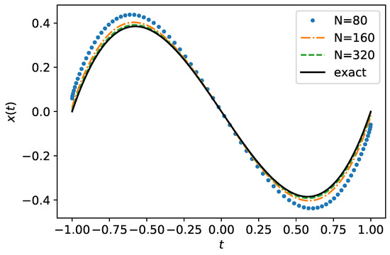
Figure 1. Numerical solutions of the Equation (54). The solid line stands for the exact solution $x^{*}\left(t\right)$.

5. Conclusions

In this paper, we constructed and justified the spline-collocation type computational scheme with first-order splines to solve the Prandtl hypersingular integral equation.

We note here a number of new approaches used for the justification of the methods and their realizations.

I.

Linear equations.

(1)

When justifying approximate methods, one usually suggests that the operator of the exact equation is continuously invertible in the corresponding Banach space.

In our work, the solvability condition of the exact equation for a given right-hand side is sufficient.

(2)

The proof of the solution convergence for an approximate scheme of a system of equations to the solution of the exact equation is based on comparing an approximation accuracy for the solution to the exact equation with the norm of the quadrature formula, which describes the numerical scheme.

The method can be regarded as analogous to the Lax–Ryabenkiy theory of difference schemes for hypersingular integral equations.

II.

Nonlinear equations.

(1)

In this paper, we provided the proof of the existence of a solution for both the exact equation and the approximate equation. The proof is based on methods of stability theory of differential equation solutions in Banach spaces. As far as the authors of this paper know, the proof of the existence of solution is based on either the Banach-type Fixed-Point Theorem (also known as the Contraction Theorem) or on the Newton–Kantorovich-type iteration methods, which require continuous invertibility of the Gateaux (Frechet) derivative at each iteration. In this work, we constructed an approximate method for solving nonlinear hypersingular integral equations, which do not require invertibility for derivatives of nonlinear operators on the entire trajectory of solution.

(2)

The justification of the convergence of the solution to an approximate method to a solution of the exact (the starting) equation is based, with the corresponding smoothness of the nonlinear operator, on comparing an estimate of the approximation accuracy of the starting equation solution with an estimate of the norm of the quadrature formula for the linear singular integral included in the starting equation. We believe that this approach seems to be new.

(3)

In this work, we presented a method of estimation of the stability area and convergence of a computational scheme.

We proposed a method to define an error estimate based on the logarithmic norm of an appropriate operator.

The method can be used to study hypersingular equations

$$a(t,x\left(t\right))+b\left(t\right)\underset{-1}{\overset{1}{\int }}\frac{x\left(\tau \right)}{{(\tau -t)}^2}d\tau +\underset{-1}{\overset{1}{\int }}\frac{h(t,\tau ,x(\tau \left)\right)}{{(\tau -t)}^2}d\tau +\underset{-1}{\overset{1}{\int }}{h}_1(t,\tau ,x\left(\tau \right))d\tau =f\left(t\right).$$

The constructed computational schemes have implemented the continuous method for solving operator equations, which are stable to perturbations of coefficients and right-hand sides.

References

- Golubev, V.V. Lectures on the Theory of the Wing; Gosudarstvennoe Izdatelstvo Tekhniko-Teoreticheskoi Literatury: Moscow, Russia, 1949; 482p. [Google Scholar]
- von Karman, T.; Burgers, J.M. General aerodynamic theory-perfect fluid. In Aerodynamic Theory; Durand, W.F., Ed.; Springer: Berlin, Germany, 1936; Volume 2. [Google Scholar]
- Schmidt, H. Strenge Lösungen zur Prandtlschen Theorie der Tragenden Linie. ZAMM 1938, 17, 101–116. [Google Scholar] [CrossRef]
- Schöder, K. Über eine Integralgleichung erster Art der Tragflügeltheorie. Sitzungsberichte Preuss Akad. D. Wiss. Phis.-Nat. Klasse 1938, 37, 345–362. [Google Scholar]
- Schöder, K. Über die Prandtlsche Integro-differentialgleichung der Trangflügeltheorie. Abhandl. D. Preuss. Akad. D. Wiss. Math. Naturwiss. Klasse 1939, 16. [Google Scholar]
- Küssner, H.; Schwartz, L. Der schwingende Flügel mit aerodynamisch ausgglichengem Ruder. Liftfahrtforschung 1949, 17, 337–354. [Google Scholar]
- Magnaradze, L.G. On a new integral equation of the theory od aircraft wings. Soob. A. N. Cruz. SSR 1942, 3, 503–508. [Google Scholar]
- Vekua, I.N. On Prandtl’s integro-differential equation. Prikl. Mat. Mech. 1945, 9, 143–150. [Google Scholar]
- Weissinger, J. Ein Satz über Fourierreichen und seine Anwendung auf die Tragflügeltheorie. Math. Zeitschr. 1940, 47, 16–33. [Google Scholar] [CrossRef]
- Belotserkovsky, S.M.; Lifanov, I.K. Method of Discrete Vortices; CRC Press: Boca Raton, FL, USA, 1992; 464p. [Google Scholar]
- Lifanov, I.K.; Poltavskii, L.N.; Vainikko, G.M. Hypersingular Integral Equations and their Applications; Chapman Hall/CRC: Boca Raton, FL, USA; London, UK, 2004. [Google Scholar]
- Bisplinghoff, L.; Ashley, H.; Halfman, R. Aeroelasticity; Dover Publications: Mineola, NY, USA, 1996. [Google Scholar]
- Blackwell, J.; Pounds, G. Wind-tunnel wall interference effect on a supercritical airfoil at transonic speeds. J. Aircr. 1977, 14, 929–935. [Google Scholar] [CrossRef]
- Bland, S.R.; Rhyne, R.H.; Pierce, H.B. A study of flow-induced vibrations of a plate in narrow channels. Trans. ASME Ser. B 1967, 89, 824–830. [Google Scholar] [CrossRef]
- Fromme, J.A.; Golberg, M.A. Numerical solution of a class of integral equations in two-dimensional aerodynamics—The problem of flaps. In Solution Methods for Integral Equations, Theory and Applications; Golberg, M.A., Ed.; Plenum Press: New York, NY, USA, 1979. [Google Scholar]
- Golberg, M.A. The numerical solution of Cauchy singular integral equations with constant coefficients. J. Int. Eq. 1985, 9, 127–151. [Google Scholar]
- Kalandia, A.I. Mathematical Methods of Two-Dimensional Elasticity; Mir: Moscow, Russia, 1975; p. 351. [Google Scholar]
- Kraft, E.; Lo, C. Analytical determination of blockage effects in a perforated wall transonic wind tunnel. AIAA J. 1977, 15, 511–516. [Google Scholar] [CrossRef]
- Ladopoulos, E.G. Singular Integral Equations. Linear and Non-Linear Theory and Its Applications in Science and Engineering; Springer: Berlin/Heidelberg, Germany, 2000. [Google Scholar]
- Lifanov, I.K. Singular Integral Equations and Discrete Vortices; VSP: Leiden, The Netherlands, 1996. [Google Scholar]
- Mokry, M. Integral equation method for subsonic flow past airfoils in ventilated wind tunnels. AIAA J. 1975, 13, 47–53. [Google Scholar] [CrossRef]
- Moss, W.F. Numerical solution of integral equations with convolution kernels. J. Int. Eq. 1982, 4, 253–264. [Google Scholar]
- Salmond, D.J. Evaluation of two-dimensional subsonic oscillatory airforce coefficients and loading distributions. Aeronaut. Quart. 1981, 32, 199–211. [Google Scholar] [CrossRef]
- Sheshko, M.A.; Rasolko, G.A.; Mastyanitsa, V.S. To the approximate solution of the integro-differential Prandtl equation. Diff. Equations 1993, 29, 1550–1560. [Google Scholar]
- Prandtl, L.; Tragflügeltheorie, I. Mitteilung Nachrichten von der Gesellschaft der Wissenschaften zu Göttingen, Mathematisch-Physikalische Klasse. 1918, 1918, 451–477. Available online: http://eudml.org/doc/59036 (accessed on 29 November 2022).
- Alexandrov, V.M.; Mkhitaryan, M.S. Contact Problems for Bodies with Thin Coatings and Interlayers; Nauka: Moscow, Russia, 1983. [Google Scholar]
- Silvestrov, V.V.; Smirnov, A.V. Integro-differential equation and a contact problem for a piecewise homogeneous plate. Appl. Math. Mech. 2010, 74, 679–691. [Google Scholar] [CrossRef]
- Muskhelishvili, N.I. Singular Integral Equations. Boundary Problems of Function Theory and Their Applications to Mathematical Physics; Aeronautical Research Laboratories: Melbourne, Australia, 1949. [Google Scholar]
- Tricomi, F. Integral Equations; N.Y. Interscience: New York, NY, USA, 1957. [Google Scholar]
- Kogan, K.M. On a singular integro-differential equation. Diff. Equations 1967, 3, 278–293. [Google Scholar]
- Koiter, W.T. On the diffusion of load from a stiffener into a sheet. Quart. J. Mech. Appl. Math. 1955, 8, 164–178. [Google Scholar] [CrossRef]
- Kalandia, A.I. On the state of stress in plates reinforced with stiffeners. J. Appl. Math. Mech. 1969, 33, 538–543. [Google Scholar] [CrossRef]
- Popov, G.Y. On the method of orthogonal polynomials in contact problems of elasticity theory. J. Appl. Math. Mech. 1969, 33, 518–531. [Google Scholar] [CrossRef]
- Muskhelishvili, N. Singular Integral Equations: Boundary Problems of Function Theory and Their Application to Mathematical Physics; Noordhoff: Leyden, The Netherlands, 1977; 447p. [Google Scholar]
- Capobianco, M.R.; Criscuolo, G.; Junghanns, P. On the Numerical Solution of a Nonlinear Integral Equation of Prandtl’s Type. Recent Adv. Oper. Theory Appl. Oper. Theory Adv. Appl. 2005, 160, 53–79. [Google Scholar]
- Ang, W.-T. Hypersingular Integral Equations in Fracture Analysis; Woodhead Publishing Limited: Sawston, UK, 2014; 204p. [Google Scholar]
- Askhabov, S.N. Nonlinear Singular Integro-Differential Equations with an Arbitrary Parameter. Mat. Zametki 2018, 103, 20–26. [Google Scholar] [CrossRef]
- Kogan, K.M.; Sakhnovich, L.A. Spectrum asymptotic one singular integro-differential equation. Diff. Equations 1984, 20, 1444–1447. [Google Scholar]
- Novin, R.; Araghi, M. Hypersingular integral equations of the first kind: A modified homotopy perturbation method and its application to vibration and active control. J. Low Freq. Noise Vib. Act. Control 2019, 38, 706–727. [Google Scholar] [CrossRef]
- Chen, Z.; Zhou, Y. A new method for solving hypersingular integral equations of the first kind. Appl. Math. Lett. 2011, 24, 636–641. [Google Scholar] [CrossRef]
- Mohammad, M.; Trounev, A. Fractional nonlinear Volterra–Fredholm integral equations involving Atangana–Baleanu fractional derivative: Framelet applications. Adv. Differ. Eq. 2020, 2020, 618. [Google Scholar] [CrossRef]
- Novin, R.; Fariborzi Araghi, M.A.; Mahmoudi, Y. Solving the Prandtl’s equation by the modified Adomian decomposition method. Commun. Adv. Comput. Sci. Appl. 2018, 2018, 9–14. [Google Scholar] [CrossRef]
- Multhopp, H. Die Berechnung der Auftriebsverteilung von Tragflugeln. Luftfahrtforschung 1938, 15, 153–169. [Google Scholar]
- Rasolko, G.A. Numerical solution of singular integro-differential Prandtl equation by the method of orthogonal polynomials. J. Belarusian State Univ. Math. Inf. 2018, 3, 68–74. [Google Scholar] [CrossRef]
- Boykov, I.V. Analytical and numerical methods for solving hypersingular integral equations. Dynamical Syst. 2019, 9, 244–272. [Google Scholar]
- Boykov, I.V.; Roudnev, V.A.; Boykova, A.I. Methods for Solving Linear and Nonlinear Hypersingular Integral Equations. Axioms 2020, 9, 74. [Google Scholar] [CrossRef]
- Boykov, I.V. Approximate Methods for Solving Hypersingular integral Equations. In Topics in Integral and Integro-Difference Equations. Theory and Applications; Singh, H., Dutta, H., Cavalcanti, M.M., Eds.; Springer: Cham, Switzerland, 2021; pp. 63–102. [Google Scholar]
- Eshkuvatov, Z.K. Semi-Bounded Solution of Hypersingular Integral Equations of the First Kind. In Proceedings of the Sixteenth Russian Conference with International Participation MCM-2022, Penza, Russia, 14 June 2022. [Google Scholar]
- Boykov, I.V.; Roudnev, V.A.; Boykova, A.I.; Baulina, O.A. New iterative method for solving linear and nonlinear hypersingular integral equations. Appl. Numer. Math. 2018, 127, 280–305. [Google Scholar] [CrossRef]
- Boikov, I.V. On a continuous method for solving nonlinear operator equations. Differ. Equations 2012, 48, 1308–1314. [Google Scholar] [CrossRef]
- Daletskii, Y.L.; Krein, M.G. Stability of Solutions of Differential Equations in Banach Space; Nauka: Moscow, Russia, 1970; 536p. [Google Scholar]
- Lozinskii, S.M. Note on a paper by V.S. Godlevskii. USSR Comput. Math. Math. Phys. 1973, 13, 232–234. [Google Scholar] [CrossRef]
- Boikov, I.V. On the stability of solutions of differential and difference equations in critical cases. Soviet Math. Dokl. 1990, 42, 630–632. [Google Scholar]
- Boykov, I.V. Optimal Function Approximation Methods and Calculation of Integrals; Publishing House of Penza State University: Penza, Russia, 2007; p. 236. [Google Scholar]
- Boykov, I.V. Approximate Methods for Evaluation of Singular and Hypersingular Integrals, Part 2, Hypersingular Integrals; Penza State University Press: Penza, Russia, 2009. (In Russian) [Google Scholar]
- Boykov, I.V.; Ventsel, E.S.; Roudnev, V.A.; Boykova, A.I. An approximate solution of nonlinear hypersingular integral equations. Appl. Numer. Math. 2014, 86, 1–21. [Google Scholar] [CrossRef]
Publisher’s Note: MDPI stays neutral with regard to jurisdictional claims in published maps and institutional affiliations. |
© 2022 by the authors. Licensee MDPI, Basel, Switzerland. This article is an open access article distributed under the terms and conditions of the Creative Commons Attribution (CC BY) license (https://creativecommons.org/licenses/by/4.0/).