K-Nearest Neighbor Estimation of Functional Nonparametric Regression Model under NA Samples

Abstract

Functional data, which provides information about curves, surfaces or anything else varying over a continuum, has become a commonly encountered type of data. The k-nearest neighbor (kNN) method, as a nonparametric method, has become one of the most popular supervised machine learning algorithms used to solve both classification and regression problems. This paper is devoted to the k-nearest neighbor (kNN) estimators of the nonparametric functional regression model when the observed variables take values from negatively associated (NA) sequences. The consistent and complete convergence rate for the proposed kNN estimator is first provided. Then, numerical assessments, including simulation study and real data analysis, are conducted to evaluate the performance of the proposed method and compare it with the standard nonparametric kernel approach.

1. Introduction

Functional data analysis (FDA) is a branch of statistics that analyzes data providing information about curves, surfaces or anything else varying over a continuum. In its most general form, under an FDA framework, each sample element of functional data is considered to be a random function.

Popularized by Ramsay and Silverman [1,2], statistics for functional data analysis have attracted considerable research interest because of its wide applications in many practical fields, such as medicine, economics and linguistics. For an introduction to the topics, we can refer to the monographs of Ramsay and Silverman [3] for parametric models, and Ferraty and Vieu [4] for nonparametric models.

In this paper, the following functional non-parametric regression model is considered.

$$Y=m\left(\chi \right)+ϵ,\left(1\right)$$

where Y is a scalar response variable, $\chi$ is a covariate taking value in a subset $S_{\mathfrak{F}}$ of an infinite-dimensional functional space $\mathfrak{F}$ endowed with a semi-metric $d(·,·)$. $m(·)$ is the unknown regression operator from $S_{\mathfrak{F}}$ to $\mathfrak{R}$, and the random error $ϵ$ satisfies $E\left(ϵ\right|\chi )=0,a.s.$

For the estimation of model (1), Ferraty and Vieu [5] investigated the classical functional Nadaraya-Watson (N-W) kernel type estimator of $m(·)$ and obtained the asymptotic properties with rates in the case of $\alpha$-mixing functional data. Ling and Wu [6] studied the modified N-W kernel estimate and derived the asymptotic distribution for strong mixing functional time series data, Baíllo and Grane [7] proposed a functional local linear estimate based on the local linear idea. In this paper, we focus on the k-nearest neighbors (kNN) method for regression model (1). The kNN method, as one of the most simple and traditional nonparametric techniques, is often used as a nonparametric classification method. The kNN method was first developed by Evelyn Fix and Joseph Hodges in 1951 [8] and then expanded by Thomas Cover [9]. In our kNN regression, the input consists of the k-closest training examples in a dataset, whereas the output is the property value for the object. This value is the average of the values of the k-nearest neighbors. Under independent samples, research in kNN regression mostly focuses on the estimation of the continuous regression function $m\left(\chi \right)$. For example, Burba et al. [10] investigated the kNN estimator based on the idea of the local adaptive bandwidth of functional explanatory variables. The papers [11,12,13,14,15,16,17,18], and others, obtained the asymptotic behavior of nonparametric regression estimators for functional data in independent and dependent cases. Further, Kudraszow and Vieu [19] obtained asymptotic results for a kNN generalized regression estimator when the observed variables take values in an abstract space. Kara-Zaitri et al. [20] provided an asymptotic theory for several different target operators and some simulated experiences, including regression, conditional density, conditional distribution and hazard operators. However, functional observations often behave with correlation, including satisfying some form of negative dependence or negative association.

Negatively associated (NA) sequences were introduced by Joag-Dev and Proschan in [21]. Random variables ${\left\{Y_i\right\}}_{1\le i\le n}$ are said to be NA, if for every pair of disjoint subsets $A,B\subset \{1,2,\dots ,n\},$

$$\mathrm{Cov}\left(f(Y_i,i\in A)g(Y_j,j\in B)\right)\le 0,$$

or equivalently,

$$\mathrm{E}(f(Y_i,i\in A),g(Y_j,j\in B))\le \mathrm{E}\left(f(Y_i,i\in A)\right)\mathrm{E}\left(g(Y_j,j\in B)\right),$$

where f and g are coordinatewise non-decreasing, such that this covariance exists. An infinite sequence ${\left\{Y_n\right\}}_{n\ge 1}$ is NA if every finite subcollection is NA.

For example, if ${\left\{Y_i\right\}}_{1\le i\le n}$ follows permutation distributions, where $\{Y_1,Y_2,\dots ,Y_n\}=\{y_1,y_2,\dots ,y_n\}$ always and $y_1\le y_2\le \dots \le y_n$ are n real numbers, then ${\left\{Y_i\right\}}_{1\le i\le n}$ is NA.

Whereas kNN regression under NA sequences has not been explored in the literature, in this paper, we extend the kNN estimation of functional data from the case of independent samples to NA sequences.

Let a pair ${\left\{({\chi }_i,Y_i)\right\}}_{i=1,\dots ,n}$ be a sample of NA pairs in $(\chi ,Y)$, which is a random vector valued in the $\mathfrak{F}\times \mathfrak{R}$. $(\mathfrak{F},d)$ is a semi-metric space, $\mathfrak{F}$ is not necessarily of the finite dimension and we do not suppose the existence of a density for the functional random variable $\chi$. For a fixed $\chi \in \mathfrak{F}$, the closed ball with $\chi$ as the center and $ϵ$ as the radius is denoted as:

$$d:B(\chi ,ϵ)=\{{\chi }^{\prime }\in \mathfrak{F}|d({\chi }^{\prime },\chi )\le ϵ\}.$$

The kNN regression estimator [10] is defined as follows:

$${\widehat{m}}_{kNN}\left(\chi \right)=\frac{{\displaystyle \sum _{i=1}^n}{Y}_{i}K\left(H_{n,k}{\left(\chi \right)}^{-1}d({\chi }_i,\chi )\right)}{{\displaystyle \sum _{i=1}^n}K\left(H_{n,k}{\left(\chi \right)}^{-1}d({\chi }_i,\chi )\right)},\chi \in \mathfrak{F},$$

(2)

where $K(·)$ is the kernel function supported on $[0,\infty )$. $H_{n,k}\left(\chi \right)$ is a positive random variable that depends on $({\chi }_1,{\chi }_2,\dots ,{\chi }_n)$ and is defined by:

$$H_{n,k}\left(\chi \right)=min\{h\in R^{+}:\sum _{i=1}^n{I}_{B(\chi ,h)}\left({\chi }_i\right)=k\},$$

obviously, the kNN estimator can be seen as an expansion to a random locally adaptive neighborhood of the traditional kernel method [5] defined as:

$${\widehat{m}}_n\left(\chi \right)=\frac{{\displaystyle \sum _{i=1}^n}{Y}_{i}K\left(h_n{\left(\chi \right)}^{-1}d({\chi }_i,\chi )\right)}{{\displaystyle \sum _{i=1}^n}K\left(h_n{\left(\chi \right)}^{-1}d({\chi }_i,\chi )\right)},\chi \in \mathfrak{F},$$

(3)

where $h_n\left(\chi \right)$ is a sequence of positive real numbers such as $h_n\left(\chi \right)\to 0$ a.s. $n\to \infty$.

This paper is organized as follows. The main results of our paper about the asymptotic behavior of the kNN estimators using a data-driven random number of neighbors are given in Section 2. Section 3 illustrates the numerical performance of the proposed method, including nonparametric functional regression analysis of the sea level surface temperature (SST) data for the El Ni$\tilde{n}$o area (0–100 S, 800–900 W). The technical proofs are postponed to Section 4. Finally, Section 5 is devoted to comments on the results and to related perspectives for the future.

2. Assumptions and Main Results

In this section, we focus on the asymptotic property of the kNN regression estimator and need to state the convergence rate of an estimator.

One says that the rate of almost complete convergence of a sequence $\{Y_n,n\ge 1\}$ to Y is of order $u_n$ if only if for any $ϵ>0$,

$$\sum _{n=1}^{\infty }P\left(\right|Y_n-Y|>ϵu_n)<\infty ,$$

and we write $Y_n-Y=O_{a.co.}\left(u_n\right)$(see for instance [5]). By the Borel-Cantelli lemma, this implies that $\frac{Y_n-Y}{u_n}\to 0$ almost surely, so almost complete convergence is a stronger result than almost sure convergence.

Our results are stated under some mild assumptions we gather below for easy references. Throughout the paper, we will denote by $C,C_1,C^{\prime }$ some positive generic constants, which may be different in various places.

Assumption 1.

$\forall ϵ>0,P(\chi \in B(\chi ,ϵ))={\phi }_{\chi }\left(ϵ\right)>0$ and ${\phi }_{\chi }(·)$ is a continuous function, and strictly monotonically increasing at the origin with ${\phi }_{\chi }\left(0\right)=0$.

Assumption 2.

There exist a function $\varphi (·)\ge 0$ and a bounded function $f(·)>0$ such that:

(i) 

F$\varphi \left(0\right)=0$, and $\underset{ϵ\to \infty }{lim}\varphi \left(ϵ\right)=0.$

(ii) 

$\underset{ϵ\to \infty }{lim}\frac{\varphi \left(uϵ\right)}{\varphi \left(ϵ\right)}=0,$ for any $u\in [0,1].$

(iii) 

$\exists \tau >0$ such that ${sup}_{\chi \in S_{\mathfrak{F}}}\left|\frac{{\phi }_{\chi }\left(ϵ\right)}{\varphi \left(ϵ\right)}-f\left(\chi \right)\right|=O\left({ϵ}^{\tau }\right),ϵ\to 0.$

Assumption 3.

$K\left(t\right)$ is a nonnegative bounded kernel function with support [0, 1], and if $K\left(1\right)>0$, the derivative $K^{{}^{\prime }}\left(t\right)$ exists on [0, 1] satisfying:

$$-\infty <C<K^{{}^{\prime }}\left(t\right)<C^{\prime }<\infty ,for\forall t\in [0,1].$$

Assumption 4.

$m(·)$ is a bounded Lipschitz operator with order β on $S_{\mathfrak{F}}$, and there exists $\beta >0$ such that:

$$\forall {\chi }_1,{\chi }_2\in S_{\mathfrak{F}},\left|m\left({\chi }_1\right)-m\left({\chi }_2\right)\right|\le Cd{({\chi }_1,{\chi }_2)}^{\beta }.$$

Assumption 5.

$\forall m\ge 2,E\left({\left|Y\right|}^m\mid X=\chi \right)={\delta }_m\left(\chi \right)<C$ with ${\delta }_m(·)$ continuous on $S_{\mathfrak{F}}.$

Assumption 6.

Kolmogorov’s ϵ-entropy of $S_{\mathfrak{F}}$ satisfies:

$$\sum _{n=1}^{\infty }exp\left\{(1-\omega ){\mathsf{\Psi }}_{S_{\mathfrak{F}}}\left(\frac{logn}{n}\right)\right\}<\infty ,forsome\omega >1.$$

For $\forall ϵ>0$, the Kolmogorov’s ϵ-entropy of some set $S_{\mathfrak{F}}\subset \mathfrak{F}$ is defined by ${\mathsf{\Psi }}_{S_{\mathfrak{F}}}=log\left(N_{ϵ}\left(S_{\mathfrak{F}}\right)\right),$ where $N_{ϵ}\left(S_{\mathfrak{F}}\right)$ is the minimal number of open balls, which can cover $S_{\mathfrak{F}}$ with ${\chi }_1,{\chi }_2,\dots ,{\chi }_{N_{ϵ}\left(S_{\mathfrak{F}}\right)}$ as the center and ϵ as the radius in $\mathfrak{F}$.

Remark 1.

Assumption 1, Assumption 2((i)–(iii)) and Assumption 4 are the standard assumptions for small ball probability and regression operators in nonparametric FDA, see Kudraszow and Vieu [19]. Assumption 2(ii) will play a key role in the methodology particularly when we compute the asymptotic variance and permit it to be explicit in Ling and Wang [6]. Assumption 2(iii) shows that the small ball probability can be written as the product of the two independent functions $\varphi (·)$ and $f(·)$, which has been used many times in Masry [11], Laib and Louani [12] and other literatures. Assumption 5 is standard in the nonparametric setting and concerns the existence of the conditional moments in Masry [11] and Burba [10], which aims to obtain the rate of uniform almost complete convergence. Assumption 6 assumes the Kolmogorov’s ϵ-entropy condition, which we will use in the following proof of the rate of uniform almost complete convergence.

Theorem 1.

Under Assumptions 1–6, suppose that sequence $\{k_n,n\ge 1\}$ satisfies $\frac{k_n}{n}\to 0,n\to \infty$, $\frac{{log}^{2}n}{k_n}<{\mathsf{\Psi }}_{S_{\mathfrak{F}}}\left(\frac{logn}{n}\right)<\frac{k_n}{logn}$ and $0<C_1<\frac{k_n}{{log}^{2}n}<C_2<\infty ,$ for n large enough, then we have:

$$\underset{\chi \in S_{\mathfrak{F}}}{sup}\left|{\widehat{m}}_{kNN}\left(\chi \right)-m\left(\chi \right)\right|=O_{a.co.}\left({\varphi }^{-1}{\left(\frac{k_n}{n}\right)}^{\beta }+\sqrt{\frac{s_n^2{\mathsf{\Psi }}_{S_{\mathfrak{F}}}\left(\frac{logn}{n}\right)}{n^2}}\right).$$

Remark 2.

The Theorem extends the kNN estimation result of Theorem 2 in Kudraszow and Vieu [19] from the independent case to the NA mixed dependent case, and obtains the same convergence rate under the assumptions. Second, the almost complete convergence rate of the prediction operator is divided into two parts, one part affected by strong mixing and Kolmogorov’s $ϵ$-entropy, and the other part depends on the smoothness of the regression operator and smoothness parameter k.

Corollary 1.

Under the condition of the Theorem, we have:

$$\underset{\chi \in S_{\mathfrak{F}}}{sup}\left|{\widehat{m}}_{kNN}\left(\chi \right)-m\left(\chi \right)\right|=O_{a.s.}\left({\varphi }^{-1}{\left(\frac{k_n}{n}\right)}^{\beta }+\sqrt{\frac{s_n^2{\mathsf{\Psi }}_{S_{\mathfrak{F}}}\left(\frac{logn}{n}\right)}{n^2}}\right).$$

Corollary 2.

Under the condition of the Theorem, we have:

$$\underset{\chi \in S_{\mathfrak{F}}}{sup}\left|{\widehat{m}}_{kNN}\left(\chi \right)-m\left(\chi \right)\right|=O_P\left({\varphi }^{-1}{\left(\frac{k_n}{n}\right)}^{\beta }+\sqrt{\frac{s_n^2{\mathsf{\Psi }}_{S_{\mathfrak{F}}}\left(\frac{logn}{n}\right)}{n^2}}\right).$$

3. Simulation

3.1. A simulation Study

In this section, we aim at illustrating the performance of the nonparametric functional regression model and we will make a comparison with traditional kernel density estimation methods. We consider the nonparametric functional regression model:

$$Y_i=m\left({\chi }_i\right)+{\epsilon }_i,$$

where $m\left({\chi }_i\right)={\left({\int }_0^{\frac{\pi }{5}}{\chi }_i^{{}^{\prime }}\left(t\right)dt\right)}^2$, ${\epsilon }_i$ is distributed according to $N(0,0.05)$, the functional curve ${\chi }_i\left(t\right)$ is generated in the following way:

$${\chi }_i\left(t\right)=a_i{t}^3+arctan\left(b_i\left(t-\frac{\pi }{5}\right)\right),t\in \left[0,\frac{\pi }{5}\right],i=1,2,\dots ,n.$$

where $\left\{a_i\right\}\sim N\left(0,\frac{\pi }{10}\right),i=1,2,\dots ,n$, $\left\{b_1,b_2,\dots ,b_n\right\}\sim N_n(\mathbf{0},\mathsf{\Sigma })$, 0 represents zero vector and the covariance matrix is defined as:

$$\sum ={\left(\begin{array}{ccccccc}1+{\theta }^2& -\theta & 0& \dots & 0& 0& 0\\ -\theta & 1+{\theta }^2& -\theta & \dots & 0& 0& 0\\ 0& -\theta & 1+{\theta }^2& \dots & 0& 0& 0\\ ⋮& ⋮& ⋮& & ⋮& ⋮& ⋮& \\ 0& 0& 0& \dots & 1+{\theta }^2& -\theta & 0\\ 0& 0& 0& \dots & -\theta & 1+{\theta }^2& -\theta \\ 0& 0& 0& \dots & 0& -\theta & 1+{\theta }^2\end{array}\right)}_{n\times n},0<\theta <1.$$

By the definition of NA, it can be seen that $(b_1,b_2,\dots ,b_n)$ is an NA vector for each $n\ge 3$ with a finite moment of any order (see Wu and Wang [22]).

We choose casually that $\theta =0.4$, the sample sizes n as $n=330$, t takes 1000 equispaced values in $[0,\frac{\pi }{5}]$. We carry out the simulation of the curve $\chi \left(t\right)$ for the 330 samples (see Figure 1).

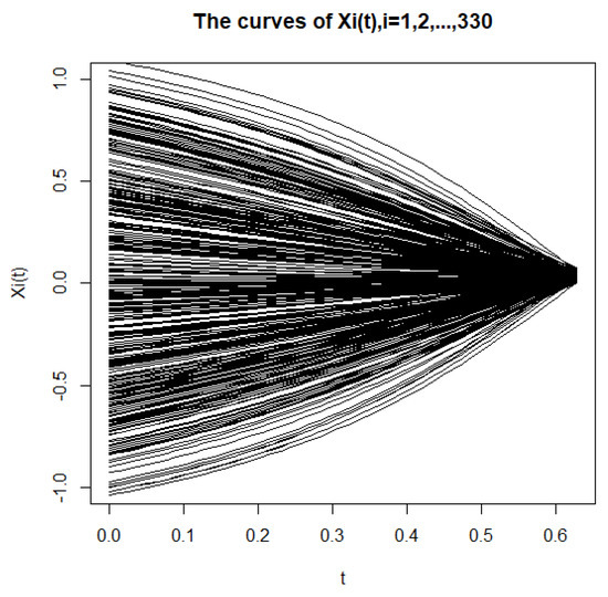
Figure 1. Curve-sample with sample size of n = 330.

We consider the Epanechnikov kernel given by $K\left(u\right)=\frac{3}{4}(1-u^2)I_{[0,1]}\left(u\right)$, and the semi-metrics $d(·,·)$ based on derivatives of order q.

$$d({\chi }_i,{\chi }_j)=\sqrt{{\int }_0^{\frac{\pi }{5}}{\left({\chi }_i^{\left(q\right)}\left(t\right)-{\chi }_j^{\left(q\right)}\left(t\right)\right)}^{2}dt},\forall {\chi }_i,{\chi }_j\in \mathfrak{F},q=\{0,1,2,\dots \}.$$

Our purpose is to compare the mean square error (MSE) of the kNN method with the NW kernel approach on finite simulated datasets. In the finite sample simulation, the following steps are followed.

Step 1: We take 300 curves to construct the training samples ${\left\{{\chi }_i,Y_i\right\}}_{i=1}^{300}$, and the other 30 constitute the test samples ${\{{\chi }_i,Y_i\}}_{i=301}^{330}$.

Step 2: In the training sample, the parameters k and h in the kNN method and NW kernel method are automatically selected based on the cross-validation method, respectively.

Step 3: Based on the MSE standard (see [4] for details), we obtain that the respective semi-metric parameters q in both the kNN method and the NW method takes $q=1$.

Step 4: The response values ${\left\{{\widehat{Y}}_i\right\}}_{i=301}^{330}$ and ${\left\{{\tilde{Y}}_i\right\}}_{i=301}^{330}$ of the test sample ${\left\{Y_i\right\}}_{i=301}^{330}$ are calculated by using the kNN method and the NW method, respectively, and their MSE and scatter plots against the true value ${\left\{Y_i\right\}}_{i=301}^{330}$ are represented by Figure 2.

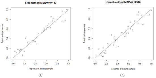
Figure 2. Prediction effects of the two estimation methods. (a) kNN estimation method. (b) NW estimation method.

As we can see in Figure 2, the MSE of the kNN method is much smaller than that of the NW method, and the scattered points in Figure 2 are more densely distributed around the linear function $y=x$, which shows that the kNN method has a better fit and higher prediction accuracy for the NA dependent functional samples.

The kNN method and NW method were used to conduct 100 independent replicated experiments at sample sizes of $n=200,300,500,800$, respectively. AMSE was calculated for both methods at different sample sizes using the following equation.

$$\mathrm{AMSE}=\frac{1}{100}\sum _{j=1}^{100}\frac{1}{30}\sum _{i=n-30}^n{\left({\overline{Y}}_i-Y_i\right)}^2,{\overline{Y}}_i={\widehat{Y}}_i,{\tilde{Y}}_i,n=200,300,500,800$$

As can be seen from Table 1, the AMSE of the kNN method is much smaller than that of the NW kernel method when the sample size is fixed at $n=200,300,500,800$, respectively; when the estimation method is fixed, the AMSE of the two estimation methods have the same trend—they both decrease as the sample size increases. However, the decreasing speed of the kNN method is significantly faster than that of the NW kernel method.

Table 1. The AMSE of the predicted response variables of the two methods under different sample sizes.

n	200	300	500	800
kNN- AMSE	0.0623	0.0470	0.0327	0.0291
NW- AMSE	0.2764	0.2593	0.2329	0.2117

3.2. A Real Study

This section applies the proposed kNN regression analysis of the data, which consist of the sea level surface temperature (SST) for the El $Ni\tilde{n}o$ area (0–100 S, 800–900 W) for a total of 31 years from 1 January 1990 to 31 December 2020. The data are available online at the website: https://www.cpc.ncep.noaa.gov/data/indices/ (accessed on 1 January 2022). More relevant discussions of these data can be found in Ezzahrioui et al. [13,14], Delsol et al. [23], and Ferraty et al. [24] The 1618 weekly SST data from the original data were preprocessed and averaged by month to obtain 372 monthly average SST discrete data. Figure 3 displays the decomposition of the multiplicative time series of the monthly SST.

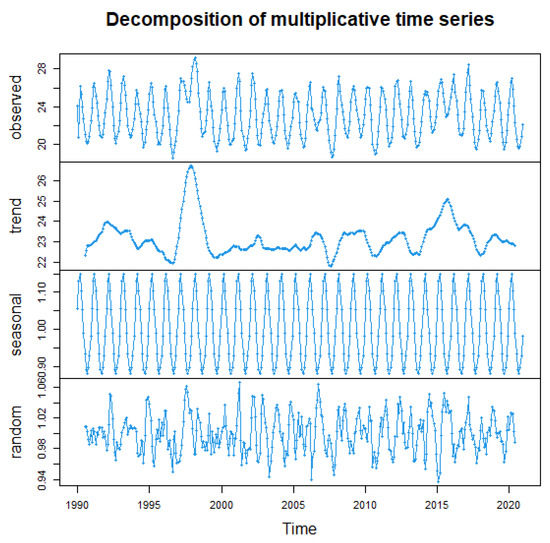
Figure 3. Monthly mean SST factor decomposition fitting comprehensive output diagram.

Figure 4 shows that the monthly average SST in El Ni$\tilde{n}$o regions from 1990 to 2020 had a clear seasonal variation, and the monthly trend of SST can also clearly be observed from the seasonal index plot of the monthly mean SST.

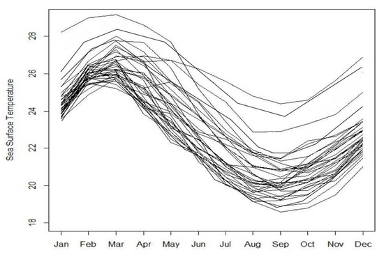
Figure 4. Time series curve of SST in El Ni$\tilde{n}$o during 31 years.

The main factors affecting the temperature variation can be generally summarized as seasonal factors and random fluctuations. If the seasonal factor is removed, the SST should be left with only random fluctuations, i.e., the values fluctuate up and down at some mean value. At the same time, if the effect of random fluctuations is not considered, the SST is left with only the seasonal factor, i.e., the SST will have similar values in the same month in different years.

The following steps implement the kNN regression estimation method for the analysis of the SST data and display the comparison with the NW sum estimation method in Figure 5.

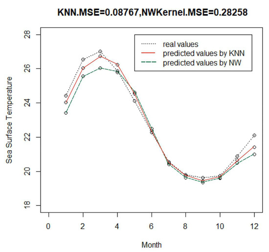
Figure 5. Forecast value of SST in 2020 by KNN method and NW method.

Step 1: Transform 372 months (31 years) of SST data $\{Z_i,i=1,\dots ,372\}$ into functional data.

Step 2: Divide the 31 samples of data ${({\chi }_j,Y_j\left(s\right))}_{j=1,\dots ,31}$ into two parts: 30 training samples of data ${({\chi }_j,Y_j\left(s\right))}_{j=1,\dots ,30}$ for model fitting and 1 test sample of data $({\chi }_{31},Y_{31}\left(s\right))$ for prediction assessment.

Step 3: Here, the functional principal component analysis (FPCA) is applicable to semi-measures for rough curves such as SST data (see Chapter 3 of Ferraty et al. [25] for the methodology). A quadratic kernel function used in Section 3.1 is used in kNN regression.

Step 4: The SST values $({\widehat{Y}}_{31}\left(s\right),s=1,\dots ,12)$ for 12 months in 2020 are predicted by the kNN method and the NW method, respectively, along with obtaining their MSEs for both methods.

Then, in step 1, we split the discrete monthly average temperature data of 372 months into 31 years of temperature profiles and express them as ${\chi }_i=\{Z_i\left(t\right),12(j-1)<t<12j\},i=1,\dots ,31$. Therefore, the response variable can be expressed as $Y_j\left(s\right)=\{Z_{12j+s},s=1,\dots ,12\}$,$j=1,\dots ,30$. Thus, ${({\chi }_j,Y_j\left(s\right))}_{j=1,\dots ,30}$ is the sample set of dependent function type with a sample size of 30, where ${\chi }_j$ is the function type data, and $Y_j\left(s\right)$ is a real value.

In Step 3, the choice of parameters q for the kNN method and NW method is performed via computation of cross-validation in R, which gives $q=3$ and $q=1$ for the kNN regression method and NW method, respectively. The selection of parameters k and h is similar to Section 3.1.

From Figure 5, which compares the MSE values calculated by the two methods, it can be seen that the MSE of the kNN method is much smaller than that of the NW method. Further, noting that the degree of fit between the curves fitted by the two methods to the true curve (dotted line), the predicted curves by two methods are generally closer to the true curve, indicating that the prediction effect of both methods is very good. However, a closer look reveals that the predicted values of the kNN method obviously have better fitting at the inflection points of the curves, such as January, February, March, November and December, which fully reflect the fact that the kNN method pays more attention to the local variation than the NW method when processing the data like this, including the abnormal or extreme distribution of the response variable.

4. Proof of Theorem

In order to prove the main results, we give some lemmas. Let ${(A_i,B_i)}_{i=1,2,\dots ,n}$ be n random pairs valued in $(\mathsf{\Omega }\times \mathfrak{R},\mathfrak{A}\times \mathfrak{B}(\mathfrak{R}\left)\right)$, where $(\mathsf{\Omega },\mathfrak{A})$ is a general measurable space. Let $S_{\mathsf{\Omega }}$ be a fixed subset of $\mathsf{\Omega }$, $G(·,(\chi ,·)):\mathfrak{R}\times (S_{\mathsf{\Omega }}\times \mathsf{\Omega })\to {\mathfrak{R}}^{+}$ be a measurable function, for $\forall t,t^{\prime }\in \mathfrak{R}$,

$$\left(L_0\right):t\le t^{\prime }\Rightarrow G(t,z)\le G(t^{\prime },z),\forall z\in S_{\mathsf{\Omega }}\times \mathsf{\Omega },$$

${D_n\left(\chi \right)}_{n\in \mathbb{N}}$ is a sequence of random real variables (r.r.v.), and $c(·):S_{\mathsf{\Omega }}\to \mathfrak{R}$ is a nonrandom function such that ${sup}_{\chi \in S_{\mathsf{\Omega }}}\left|c\left(\chi \right)\right|<\infty$. For $\forall \chi \in S_{\mathsf{\Omega }},n\in \mathbb{N}/\left\{0\right\}$, we define:

$$c_{n,\chi }\left(t\right)=\frac{{\displaystyle \sum _{i=1}^n}{B}_{i}G(t,(\chi ,A_i))}{{\displaystyle \sum _{i=1}^n}G(t,(\chi ,A_i))}.$$

Lemma 1

([10]). Let ${u_n\left(\chi \right)}_{n\in \mathbb{N}}$ be a decreasing positive real sequence satisfying ${lim}_{n\to \infty }{u}_n=0$. For any increasing sequences ${\beta }_n\in (0,1)$ and ${\beta }_n-1=O\left(u_n\right)$, there exist two real random sequences ${\left\{D_n^{-}({\beta }_n,\chi )\right\}}_{n\in \mathbb{N}}$ and ${\left\{D_n^{+}({\beta }_n,\chi )\right\}}_{n\in \mathbb{N}}$ such that:

(L1) 

$D_n^{-}({\beta }_n,\chi )\le D_n^{+}({\beta }_n,\chi ),\forall n\in \mathbb{N},\forall \chi \in S_{\mathsf{\Omega }}$,

(L2) 

$I_{\left\{D_n^{-}({\beta }_n,\chi )\le D_n({\beta }_n,\chi )\le D_n^{+}({\beta }_n,\chi ),\forall \chi \in S_{\mathsf{\Omega }}\right\}}\to 1,$ a.co. $n\to \infty ,$

(L3) 

${sup}_{\chi \in S_{\mathsf{\Omega }}}\left|\frac{{\displaystyle \sum _{i=1}^n}G\left(D_n^{-}({\beta }_n,\chi )\right)}{{\displaystyle \sum _{i=1}^n}G\left(D_n^{+}({\beta }_n,\chi )\right)}-{\beta }_n\right|=O_{a.co.}\left(u_n\right),$

(L4) 

${sup}_{\chi \in S_{\mathsf{\Omega }}}\left|c_{n,\chi }\left(D_n^{-}({\beta }_n,\chi )\right)-c\left(\chi \right)\right|=O_{a.co.}\left(u_n\right),$

(L5) 

${sup}_{\chi \in S_{\mathsf{\Omega }}}\left|c_{n,\chi }\left(D_n^{+}({\beta }_n,\chi )\right)-c\left(\chi \right)\right|=O_{a.co.}\left(u_n\right),$

then, we have:

$$\underset{\chi \in S_{\mathsf{\Omega }}}{sup}\left|c_{n,\chi }\left(D_n({\beta }_n,\chi )\right)-c\left(\chi \right)\right|=O_{a.co.}\left(u_n\right).$$

The proof of Lemma 1 is not presented here because it follows, step by step, the same argument in Burba et al. [10], Kudraszow and Vieu [19].

Lemma 2

([26]). Let $\{X_n,n\in \mathbb{N}\}$ be an NA random sequence with zero mean, and there exists a positive constant $c_k,k=1,2,\dots ,n$ such that $|X_k|\le c_k$, let $S_n=X_1+X_2+\dots +X_n$. For any $ϵ>0$, we get:

$$P(S_n\ge nϵ)\le exp\left\{\frac{-n^2{ϵ}^2}{2{\displaystyle \sum _{i=1}^n}{c}_i^2}\right\},$$

(4)

and

$$P\left(\right|S_n|\ge nϵ)\le 2exp\left\{\frac{-n^2{ϵ}^2}{2{\displaystyle \sum _{i=1}^n}{c}_i^2}\right\}.$$

Lemma 3.

Suppose that Assumptions 1–6 hold, and $h_n\left(\chi \right)\to 0$ a.s. $n\to \infty$ in model (3) satisfying:

$$lim\left({\phi }_{\chi }\left(H_{n,k}\left(\chi \right)\right)-{\phi }_{\chi }\left(h_n\left(\chi \right)\right)\right)=0,$$

(5)

$$0<C_1{h}_n\le \underset{\chi \in S_{\mathfrak{F}}}{inf}{h}_n\left(\chi \right)\le \underset{\chi \in S_{\mathfrak{F}}}{sup}{h}_n\left(\chi \right)\le C_2{h}_n<\infty ,$$

(6)

and for n large enough,

$$\frac{{log}^{2}n}{n\varphi \left(h_n\right)}<{\mathsf{\Psi }}_{S_{\mathfrak{F}}}\left(\frac{logn}{n}\right)<\frac{n\varphi \left(h_n\right)}{logn},$$

(7)

$$0<C_1<\frac{n\varphi \left(h_n\right)}{{log}^{2}n}<C_2<\infty ,$$

(8)

then we have:

$$\underset{\chi \in S_{\mathfrak{F}}}{sup}\left|{\widehat{m}}_n\left(\chi \right)-m\left(\chi \right)\right|=O_{a.co.}\left(h_n^{\beta }\right)+O_{a.co.}\left(\sqrt{\frac{s_n^2{\mathsf{\Psi }}_{S_{\mathfrak{F}}}\left(ϵ\right)}{n^2}}\right),$$

(9)

where $ϵ=\frac{logn}{n}.$

Proof of Lemma 3. 

In order to simplify the proof, we introduce some notations in this article. For $\forall \chi \in S_{\mathfrak{F}}$, let $k\left(\chi \right)=arg\underset{k=1,2,\dots ,N_{ϵ}\left(S_{\mathfrak{F}}\right)}{min}d(\chi ,{\chi }_k)$, $s_n^2=max\left\{s_{n,1}^2,s_{n,2}^2,s_{n,3}^2,s_{n,4}^2\right\}$ be the mixed operator covariance,

$$s_{n,1}^2=\sum _{i=1}^n\sum _{j=1}^n\left|\mathrm{Cov}(Y_i{u}_i,Y_j{u}_j)\right|,s_{n,2}^2=\sum _{i=1}^n\sum _{j=1}^n\left|\mathrm{Cov}(v_i,v_j)\right|,$$

$$s_{n,3}^2=\sum _{i=1}^n\sum _{j=1}^n\left|\mathrm{Cov}(u_i,u_j)\right|,s_{n,4}^2=\sum _{i=1}^n\sum _{j=1}^n\left|\mathrm{Cov}(w_i,w_j)\right|,$$

where $u_i=I_{B\left({\chi }_{k_{\chi }},C_2{h}_n\left(\chi \right)+ϵ\right)}$, $0<h_n\to 0,$

$$v_i=\frac{Y_{i}K\left(h_n{\left({\chi }_k\right)}^{-1}d({\chi }_k,{\chi }_i)\right)}{EK\left(h_n{\left({\chi }_k\right)}^{-1}d({\chi }_k,{\chi }_1)\right)}-\frac{E\left(Y_{i}K(h_n{\left({\chi }_k\right)}^{-1}d({\chi }_k,{\chi }_i)\right)}{EK\left(h_n{\left({\chi }_k\right)}^{-1}d({\chi }_k,{\chi }_1)\right)},$$

$$w_i=\frac{K\left(h_n{\left({\chi }_k\right)}^{-1}d({\chi }_k,{\chi }_i)\right)}{EK\left(h_n{\left({\chi }_k\right)}^{-1}d({\chi }_k,{\chi }_1)\right)}-\frac{EK\left(h_n{\left({\chi }_k\right)}^{-1}d({\chi }_k,{\chi }_i)\right)}{EK\left(h_n{\left({\chi }_k\right)}^{-1}d({\chi }_k,{\chi }_1)\right)}.$$

For the fixed $\chi \in S_{\mathfrak{F}}$ in model (3), we have the decomposition as follows:

$$\begin{array}{cc}\hfill {\widehat{m}}_n\left(\chi \right)-m\left(\chi \right)& =\frac{{\widehat{m}}_{2n}\left(\chi \right)}{{\widehat{m}}_{1n}\left(\chi \right)}-m_n\left(\chi \right)\hfill \\ & =\frac{1}{{\widehat{m}}_{1n}\left(\chi \right)}[{\widehat{m}}_{2n}\left(\chi \right)-E{\widehat{m}}_n\left(\chi \right)]+\frac{1}{{\widehat{m}}_{1n}\left(\chi \right)}[E{\widehat{m}}_n\left(\chi \right)-m_n\left(\chi \right)]\hfill \\ & +\frac{m_n\left(\chi \right)}{{\widehat{m}}_{1n}\left(\chi \right)}[1-{\widehat{m}}_{1n}\left(\chi \right)].\hfill \end{array}$$

where:

$${\widehat{m}}_{1n}\left(\chi \right)=\frac{{\displaystyle \sum _{i=1}^n}K\left(h_n{\left(\chi \right)}^{-1}d(\chi ,{\chi }_i)\right)}{nEK\left(h_n{\left(\chi \right)}^{-1}d(\chi ,{\chi }_1)\right)},{\widehat{m}}_{2n}\left(\chi \right)=\frac{{\displaystyle \sum _{i=1}^n}{Y}_{i}K\left(h_n{\left(\chi \right)}^{-1}d(\chi ,{\chi }_i)\right)}{nEK\left(h_n{\left(\chi \right)}^{-1}d(\chi ,{\chi }_1)\right)}.$$

It suffices to prove the three following results in order to establish (9),

$$\underset{\chi \in S_{\mathfrak{F}}}{sup}\left|E{\widehat{m}}_{2n}\left(\chi \right)-m\left(\chi \right)\right|=O_{a.co.}\left(h_n^{\beta }\right),$$

(10)

$$\underset{\chi \in S_{\mathfrak{F}}}{sup}\left|{\widehat{m}}_{2n}\left(\chi \right)-E{\widehat{m}}_{2n}\left(\chi \right)\right|=O_{a.co.}\left(\sqrt{\frac{s_n^2{\mathsf{\Psi }}_{S_{\mathfrak{F}}}\left(ϵ\right)}{n^2}}\right),$$

(11)

$$\underset{\chi \in S_{\mathfrak{F}}}{sup}\left|{\widehat{m}}_{1n}\left(\chi \right)-1\right|=\underset{\chi \in S_F}{sup}\left|{\widehat{m}}_{1n}\left(\chi \right)-E{\widehat{m}}_{1n}\left(\chi \right)\right|=O_{a.co.}\left(\sqrt{\frac{s_n^2{\mathsf{\Psi }}_{S_{\mathfrak{F}}}\left(ϵ\right)}{n^2}}\right).$$

(12)

As to the Equation (10). For $\chi \in S_{\mathfrak{F}}$, by the Equation (6) and Assumption 4, it follows that:

$$\begin{array}{cc}\hfill \left|E{\widehat{m}}_{2n}\left(\chi \right)-m\left(\chi \right)\right|& =\left|E\frac{{\displaystyle \sum _{i=1}^n}{Y}_{i}K\left(h_n{\left(\chi \right)}^{-1}d(\chi ,{\chi }_i)\right)}{nEK\left(h_n{\left(\chi \right)}^{-1}d(\chi ,{\chi }_1)\right)}-m\left(\chi \right)\right|\hfill \\ & =\left|\frac{E{Y}_{1}K\left(h_n{\left(\chi \right)}^{-1}d(\chi ,{\chi }_i)\right)}{EK\left(h_n{\left(\chi \right)}^{-1}d(\chi ,{\chi }_1)\right)}-m\left(\chi \right)\right|\hfill \\ & =\left|\frac{m\left({\chi }_1\right)EK\left(h_n{\left(\chi \right)}^{-1}d(\chi ,{\chi }_i)\right)-m\left(\chi \right)EK\left(h_n{\left(\chi \right)}^{-1}d(\chi ,{\chi }_1)\right)}{EK\left(h_n{\left(\chi \right)}^{-1}d(\chi ,{\chi }_1)\right)}\right|\hfill \\ & =\left|m\left({\chi }_1\right)-m\left(\chi \right)\right|=O_{a.co.}\left(h_n^{\beta }\right).\hfill \end{array}$$

Then, we need to show the Equation (11). In fact, we have the decomposition as follows:

$$\begin{array}{cc}& \underset{\chi \in S_{\mathfrak{F}}}{sup}\left|{\widehat{m}}_{2n}\left(\chi \right)-E{\widehat{m}}_{2n}\left(\chi \right)\right|\hfill \\ & \le \underset{\chi \in S_{\mathfrak{F}}}{sup}\left|{\widehat{m}}_{2n}\left(\chi \right)-{\widehat{m}}_{2n}\left({\chi }_{k\left(\chi \right)}\right)\right|+\underset{\chi \in S_{\mathfrak{F}}}{sup}\left|{\widehat{m}}_{2n}\left({\chi }_{k\left(\chi \right)}\right)-E{\widehat{m}}_{2n}\left({\chi }_{k\left(\chi \right)}\right)\right|\hfill \\ & +\underset{\chi \in S_{\mathfrak{F}}}{sup}\left|E{\widehat{m}}_{2n}\left({\chi }_{k\left(\chi \right)}\right)-E{\widehat{m}}_{2n}\left(\chi \right)\right|=:I_1+I_2+I_3.\hfill \end{array}$$

For $I_1$, by Assumption 3, it is easily seen that:

$$0<C_1<EK\left(h_n{\left(\chi \right)}^{-1}d(\chi ,{\chi }_i)\right)<C_2<\infty ,$$

thus,

$$\begin{array}{cc}\hfill I_1& =\underset{\chi \in S_{\mathfrak{F}}}{sup}\left|\frac{{\displaystyle \sum _{i=1}^n}{Y}_{i}K\left(h_n{\left(\chi \right)}^{-1}d(\chi ,{\chi }_i)\right)}{nEK\left(h_n{\left(\chi \right)}^{-1}d(\chi ,{\chi }_1)\right)}-\frac{{\displaystyle \sum _{i=1}^n}{Y}_{i}K\left(h_n{\left({\chi }_{k\left(\chi \right)}\right)}^{-1}d({\chi }_{k\left(\chi \right)},{\chi }_i)\right)}{nEK\left(h_n{\left({\chi }_{k\left(\chi \right)}\right)}^{-1}d({\chi }_{k\left(\chi \right)},{\chi }_1)\right)}\right|\hfill \\ & =\underset{\chi \in S_{\mathfrak{F}}}{sup}\frac{1}{n}\sum _{i=1}^n{Y}_i\left|\frac{K\left(h_n{\left(\chi \right)}^{-1}d(\chi ,{\chi }_i)\right)}{EK\left(h_n{\left(\chi \right)}^{-1}d(\chi ,{\chi }_1)\right)}-\frac{K\left(h_n{\left({\chi }_{k\left(\chi \right)}\right)}^{-1}d({\chi }_{k\left(\chi \right)},{\chi }_i)\right)}{EK\left(h_n{\left({\chi }_{k\left(\chi \right)}\right)}^{-1}d({\chi }_{k\left(\chi \right)},{\chi }_1)\right)}\right|\hfill \\ & \le C\underset{\chi \in S_{\mathfrak{F}}}{sup}\frac{1}{n}\sum _{i=1}^n{Y}_i\left|K\left(\frac{d(\chi ,{\chi }_i)}{h_n\left(\chi \right)}\right)-K\left(\frac{d({\chi }_{k\left(\chi \right)},{\chi }_i)}{h_n\left({\chi }_{k\left(\chi \right)}\right)}\right)\right|I_{B\left(\chi ,h_n\left(\chi \right)\right)\cup B\left({\chi }_{k\left(\chi \right)},h_n\left(\chi \right)\right)}\left({\chi }_i\right)\hfill \\ & \le C\underset{\chi \in S_{\mathfrak{F}}}{sup}\frac{1}{n}\sum _{i=1}^n{Y}_i{I}_{B\left({\chi }_{k\left(\chi \right)},C_2{h}_n\left(\chi \right)+ϵ\right)}\left({\chi }_i\right),\hfill \end{array}$$

for $\forall \eta >0$, we have:

$$\begin{array}{cc}& P\left(I_1>\eta \sqrt{\frac{s_{n,1}^2{\mathsf{\Psi }}_{S_{\mathfrak{F}}}\left(ϵ\right)}{n^2}}\right)\hfill \\ & \le P\left(C\underset{\chi \in S_{\mathfrak{F}}}{sup}\frac{1}{n}\sum _{i=1}^n{Y}_i{I}_{B\left({\chi }_{k\left(\chi \right)},C_2{h}_n\left(\chi \right)+ϵ\right)}\left({\chi }_i\right)>\eta \sqrt{\frac{s_{n,1}^2{\mathsf{\Psi }}_{S_{\mathfrak{F}}}\left(ϵ\right)}{n^2}}\right)\hfill \\ & \le C{N}_{ϵ}\left(S_{\mathfrak{F}}\right)\underset{k\in \left\{{\chi }_1,{\chi }_2,\dots ,{\chi }_{N_{ϵ}\left(S_{\mathfrak{F}}\right)}\right\}}{max}P\left(\sum _{i=1}^n\left|Y_i\right|I_{B\left({\chi }_{k\left(\chi \right)},C_2{h}_n\left(\chi \right)+ϵ\right)}\left({\chi }_i\right)>\eta \sqrt{s_{n,1}^2{\mathsf{\Psi }}_{S_{\mathfrak{F}}}\left(ϵ\right)}\right).\hfill \end{array}$$

According to (4) in Lemma 2 and Assumption 6, we have:

$$\begin{array}{cc}& P\left(\sum _{i=1}^n\left|Y_i\right|I_{B\left({\chi }_{k\left(\chi \right)},C_2{h}_n\left(\chi \right)+ϵ\right)}\left({\chi }_i\right)>\eta \sqrt{s_{n,1}^2{\mathsf{\Psi }}_{S_{\mathfrak{F}}}\left(ϵ\right)}\right)\hfill \\ & \le exp\left\{\frac{-\eta s_{n,1}^2{\mathsf{\Psi }}_{S_{\mathfrak{F}}}\left(ϵ\right)}{2{\displaystyle \sum _{i=1}^n}{c}_i^2}\right\}\le exp\left\{\left(1-\frac{-\eta s_{n,1}^2}{2{\displaystyle \sum _{i=1}^n}{c}_i^2}\right)-{\mathsf{\Psi }}_{S_{\mathfrak{F}}}\left(ϵ\right)\right\}<\infty .\hfill \end{array}$$

Hence, it follows that:

$$I_1=O_{a.co.}\left(\sqrt{\frac{s_{n,1}^2{\mathsf{\Psi }}_{S_{\mathfrak{F}}}\left(ϵ\right)}{n^2}}\right).$$

(13)

For $I_2$, similar to the proof of $I_1$, for $\forall \eta >0$, we have:

$$\begin{array}{cc}& P\left(I_2>\eta \sqrt{\frac{s_{n,2}^2{\mathsf{\Psi }}_{S_{\mathfrak{F}}}\left(ϵ\right)}{n^2}}\right)\hfill \\ & =P\left(\underset{\chi \in S_{\mathfrak{F}}}{sup}\left|\frac{{\displaystyle \sum _{i=1}^n}{Y}_{i}K\left(\frac{d\left({\chi }_{k\left(\chi \right)},{\chi }_i\right)}{h_n\left({\chi }_{k\left(\chi \right)}\right)}\right)}{nEK\left(\frac{d\left({\chi }_{k\left(\chi \right)},{\chi }_1\right)}{h_n\left({\chi }_{k\left(\chi \right)}\right)}\right)}-\frac{E{\displaystyle \sum _{i=1}^n}{Y}_{i}K\left(\frac{d\left({\chi }_{k\left(\chi \right)},{\chi }_i\right)}{h_n\left({\chi }_{k\left(\chi \right)}\right)}\right)}{nEK\left(\frac{d\left({\chi }_{k\left(\chi \right)},{\chi }_1\right)}{h_n\left({\chi }_{k\left(\chi \right)}\right)}\right)}\right|>\eta \sqrt{\frac{s_{n,2}^2{\mathsf{\Psi }}_{S_{\mathfrak{F}}}\left(ϵ\right)}{n^2}}\right)\hfill \\ & =P\left(\underset{\chi \in S_{\mathfrak{F}}}{sup}\frac{1}{n}\sum _{i=1}^n\left|\frac{Y_{i}K\left(\frac{d\left({\chi }_{k\left(\chi \right)},{\chi }_i\right)}{h_n\left({\chi }_{k\left(\chi \right)}\right)}\right)}{EK\left(\frac{d\left({\chi }_{k\left(\chi \right)},{\chi }_1\right)}{h_n\left({\chi }_{k\left(\chi \right)}\right)}\right)}-\frac{E{Y}_{i}K\left(\frac{d\left({\chi }_{k\left(\chi \right)},{\chi }_i\right)}{h_n\left({\chi }_{k\left(\chi \right)}\right)}\right)}{EK\left(\frac{d\left({\chi }_{k\left(\chi \right)},{\chi }_1\right)}{h_n\left({\chi }_{k\left(\chi \right)}\right)}\right)}\right|>\eta \sqrt{\frac{s_{n,2}^2{\mathsf{\Psi }}_{S_{\mathfrak{F}}}\left(ϵ\right)}{n^2}}\right)\hfill \\ & \le N_{ϵ}\left(S_{\mathfrak{F}}\right)\underset{k\in \left\{{\chi }_1,{\chi }_2,\dots ,{\chi }_{N_{ϵ}\left(S_{\mathfrak{F}}\right)}\right\}}{max}P\left(\frac{1}{n}\sum _{i=1}^n\left|\frac{Y_{i}K\left(\frac{d\left({\chi }_{k\left(\chi \right)},{\chi }_i\right)}{h_n\left({\chi }_{k\left(\chi \right)}\right)}\right)}{EK\left(\frac{d\left({\chi }_{k\left(\chi \right)},{\chi }_1\right)}{h_n\left({\chi }_{k\left(\chi \right)}\right)}\right)}-\frac{E{Y}_{i}K\left(\frac{d\left({\chi }_{k\left(\chi \right)},{\chi }_i\right)}{h_n\left({\chi }_{k\left(\chi \right)}\right)}\right)}{EK\left(\frac{d\left({\chi }_{k\left(\chi \right)},{\chi }_1\right)}{h_n\left({\chi }_{k\left(\chi \right)}\right)}\right)}\right|>\eta \sqrt{\frac{s_{n,2}^2{\mathsf{\Psi }}_{S_{\mathfrak{F}}}\left(ϵ\right)}{n^2}}\right)\hfill \\ & \le C{N}_{ϵ}\left(S_{\mathfrak{F}}\right)\underset{k\in \left\{{\chi }_1,{\chi }_2,\dots ,{\chi }_{N_{ϵ}\left(S_{\mathfrak{F}}\right)}\right\}}{max}P\left(\frac{1}{n}\sum _{i=1}^n\left|Y_i\right|I_{B\left({\chi }_{k\left(\chi \right)},C_2{h}_n\left(\chi \right)+ϵ\right)}\left({\chi }_i\right)>\eta \sqrt{\frac{s_{n,2}^2{\mathsf{\Psi }}_{S_{\mathfrak{F}}}\left(ϵ\right)}{n^2}}\right).\hfill \end{array}$$

Thus,

$$I_2=O_{a.co.}\left(\sqrt{\frac{s_{n,2}^2{\mathsf{\Psi }}_{S_{\mathfrak{F}}}\left(ϵ\right)}{n^2}}\right).$$

(14)

Finally, for $I_3$, we can get $I_3\le E\left({sup}_{\chi \in S_{\mathfrak{F}}}\left|{\widehat{m}}_{2n}\left({\chi }_{k\left(\chi \right)}\right)-{\widehat{m}}_{2n}\left(\chi \right)\right|\right)$. The proof process is similar to $I_1$, and we can obtain:

$$I_3=O_{a.co.}\left(\sqrt{\frac{s_{n,1}^2{\mathsf{\Psi }}_{S_{\mathfrak{F}}}\left(ϵ\right)}{n^2}}\right).$$

(15)

Therefore, combining the Equations (13)–(15), the Equation (11) can be established.

Similarly, we may prove the Equation (12). Hence, the proof of Lemma 3 is completed. □

Proof of Theorem 1. 

According to Lemma 1, let $S_{\mathsf{\Omega }}=S_{\mathfrak{F}}$, $A_i={\chi }_i$, $B_i=Y_i$, $G(t,(\chi ,A_i))=K\left(t^{-1}d(\chi ,{\chi }_i)\right)$, $D_n\left(\chi \right)=H_{n,k}\left(\chi \right)$, $c_{n,\chi }\left(\chi \right)={\widehat{m}}_{kNN}\left(\chi \right)$, $c\left(\chi \right)={\widehat{m}}_n\left(\chi \right)$. Let ${\beta }_n\in (0,1)$ be an increasing sequence such that ${\beta }_n-1=O\left(u_n\right)$, where $u_n={\varphi }^{-1}{\left(\frac{k_n}{n}\right)}^{\beta }+\sqrt{\frac{s_n^2{\mathsf{\Psi }}_{S_{\mathfrak{F}}}\left(\frac{logn}{n}\right)}{n^2}}$ is a decreasing positive real sequence such that ${lim}_{n\to \infty }{u}_n=0$ and $h_n={\varphi }^{-1}{\left(\frac{k_n}{n}\right)}^{\beta }$. Let ${\left\{D_n^{-}({\beta }_n,\chi )\right\}}_{n\in \mathbb{N}}$ and ${\left\{D_n^{+}({\beta }_n,\chi )\right\}}_{n\in \mathbb{N}}$ be two real random sequences such that:

$${\phi }_{\chi }\left(D_n^{-}({\beta }_n,\chi )\right)={\phi }_{\chi }\left(h_n\left(\chi \right)\right){\beta }_n^{\frac{1}{2}},$$

(16)

$${\phi }_{\chi }\left(D_n^{+}({\beta }_n,\chi )\right)={\phi }_{\chi }\left(h_n\left(\chi \right)\right){\beta }_n^{-\frac{1}{2}},$$

(17)

Firstly, we verify the conditions $\left(L_4\right)$ and $\left(L_5\right)$ in Lemma 1. By ${\phi }_{\chi }\left(D_n^{-}({\beta }_n,\chi )\right)$ and ${\beta }_n-1=O\left(u_n\right)$, it is easy to follow that the local bandwidth $D_n^{-}({\beta }_n,\chi )$ satisfies the condition (5). Combining $h_n={\varphi }^{-1}{\left(\frac{k_n}{n}\right)}^{\beta }$ with Assumption 2, it follows that $h_n\left(\chi \right)$ satisfies the condition (6). Let $k_n=n\varphi \left(h_n\right)$, from Assumption 2(i) we obtain that $\frac{k_n}{n}=\frac{n\varphi \left(h_n\right)}{n}=n\varphi \left(h_n\right)$ is satisfied. Hence, according to the conditions of the Theorem, the Equations (7) and (8) in Lemma 3 hold. Thus, by Lemma 3, we have:

$$\underset{\chi \in S_{\mathfrak{F}}}{sup}\left|c_{n,\chi }\left(D_n^{-}({\beta }_n,\chi )\right)-c\left(\chi \right)\right|=O_{a.co.}\left({\varphi }^{-1}{\left(\frac{k_n}{n}\right)}^{\beta }+\sqrt{\frac{s_n^2{\mathsf{\Psi }}_{S_{\mathfrak{F}}}\left(\frac{logn}{n}\right)}{n^2}}\right)=O_{a.co.}\left(u_n\right).$$

Similarly, for $D_n^{+}({\beta }_n,\chi )$, we can also get:

$$\underset{\chi \in S_{\mathfrak{F}}}{sup}\left|c_{n,\chi }\left(D_n^{+}({\beta }_n,\chi )\right)-c\left(\chi \right)\right|=O_{a.co.}\left({\varphi }^{-1}{\left(\frac{k_n}{n}\right)}^{\beta }+\sqrt{\frac{s_n^2{\mathsf{\Psi }}_{S_{\mathfrak{F}}}\left(\frac{logn}{n}\right)}{n^2}}\right)=O_{a.co.}\left(u_n\right).$$

Secondly, checking the conditions $\left(L_1\right)$ and $\left(L_2\right)$ in Lemma 1, and combining (16) and (17) with ${\beta }_n\in (0,1)$, it is clearly followed that:

$${\phi }_{\chi }\left(D_n^{-}({\beta }_n,\chi )\right)\le {\phi }_{\chi }\left(h_n\left(\chi \right)\right)\le {\phi }_{\chi }\left(D_n^{+}({\beta }_n,\chi )\right),$$

(18)

By Assumption 1 we get:

$$D_n^{-}({\beta }_n,\chi )\le h_n\left(\chi \right)\le D_n^{+}({\beta }_n,\chi ).$$

According to (5) and (18), for $n\to \infty$, we have:

$${\phi }_{\chi }\left(D_n^{-}({\beta }_n,\chi )\right)\le {\phi }_{\chi }\left(H_{n,\chi }\left(\chi \right)\right)\le {\phi }_{\chi }\left(D_n^{+}({\beta }_n,\chi )\right),$$

That is:

$${\phi }_{\chi }\left(D_n^{-}({\beta }_n,\chi )\right)\le {\phi }_{\chi }\left(D_n\left(\chi \right)\right)\le {\phi }_{\chi }\left(D_n^{+}({\beta }_n,\chi )\right),$$

Therefore, by Assumption 1 we can get:

$$D_n^{-}({\beta }_n,\chi )\le D_n\left(\chi \right)\le D_n^{+}({\beta }_n,\chi ),$$

Thus,

$$I_{\left\{D_n^{-}({\beta }_n,\chi )\le D_n({\beta }_n,\chi )\le D_n^{+}({\beta }_n,\chi ),\forall \chi \in S_{\mathfrak{F}}\right\}}\to 1,a.co.n\to \infty .$$

$\left(L_2\right)$ is checked.

Finally, we establish the condition $\left(L_3\right)$ in Lemma 1. Similar to Kudraszow and Vieu [19], we denote:

$$f^{*}(\chi ,h_n\left(\chi \right))=EK\left(h_n{\left(\chi \right)}^{-1}d(\chi ,{\chi }_1)\right),\forall \chi \in S_{\mathfrak{F}}.$$

and let:

$$F_1=\frac{f^{*}\left(\chi ,D_n^{-}({\beta }_n,\chi )\right)}{f^{*}\left(\chi ,D_n^{+}({\beta }_n,\chi )\right)},F_2=\frac{{\widehat{m}}_{1n}\left(\chi ,D_n^{-}({\beta }_n,\chi )\right)}{{\widehat{m}}_{1n}\left(\chi ,D_n^{+}({\beta }_n,\chi )\right)}-1,F_3=\frac{f^{*}\left(\chi ,D_n^{+}({\beta }_n,\chi )\right)}{f^{*}\left(\chi ,D_n^{-}({\beta }_n,\chi )\right)}{\beta }_n-1.$$

Then, $\left(L_3\right)$ can be decomposed as follows:

$$\begin{array}{cc}& \underset{\chi \in S_{\mathfrak{F}}}{sup}\left|\frac{{\displaystyle \sum _{i=1}^n}G\left(D_n^{-}({\beta }_n,\chi )\right)}{{\displaystyle \sum _{i=1}^n}G\left(D_n^{+}({\beta }_n,\chi )\right)}-{\beta }_n\right|\hfill \\ & =\left|\frac{{\widehat{m}}_{1n}\left(\chi ,D_n^{-}({\beta }_n,\chi )\right)}{{\widehat{m}}_{1n}\left(\chi ,D_n^{+}({\beta }_n,\chi )\right)}\frac{f^{*}\left(\chi ,D_n^{-}({\beta }_n,\chi )\right)}{f^{*}\left(\chi ,D_n^{+}({\beta }_n,\chi )\right)}-\frac{f^{*}\left(\chi ,D_n^{+}({\beta }_n,\chi )\right)}{f^{*}\left(\chi ,D_n^{-}({\beta }_n,\chi )\right)}\frac{f^{*}\left(\chi ,D_n^{-}({\beta }_n,\chi )\right)}{f^{*}\left(\chi ,D_n^{+}({\beta }_n,\chi )\right)}{\beta }_n\right|\hfill \\ & =\left|\frac{f^{*}\left(\chi ,D_n^{-}({\beta }_n,\chi )\right)}{f^{*}\left(\chi ,D_n^{+}({\beta }_n,\chi )\right)}\right|\left|\frac{{\widehat{m}}_{1n}\left(\chi ,D_n^{-}({\beta }_n,\chi )\right)}{{\widehat{m}}_{1n}\left(\chi ,D_n^{+}({\beta }_n,\chi )\right)}-\frac{f^{*}\left(\chi ,D_n^{+}({\beta }_n,\chi )\right)}{f^{*}\left(\chi ,D_n^{-}({\beta }_n,\chi )\right)}{\beta }_n\right|\hfill \\ & \le \left|\frac{f^{*}\left(\chi ,D_n^{-}({\beta }_n,\chi )\right)}{f^{*}\left(\chi ,D_n^{+}({\beta }_n,\chi )\right)}\right|\left(\left|\frac{{\widehat{m}}_{1n}\left(\chi ,D_n^{-}({\beta }_n,\chi )\right)}{{\widehat{m}}_{1n}\left(\chi ,D_n^{+}({\beta }_n,\chi )\right)}-1\right|+\left|\frac{f^{*}\left(\chi ,D_n^{+}({\beta }_n,\chi )\right)}{f^{*}\left(\chi ,D_n^{-}({\beta }_n,\chi )\right)}{\beta }_n-1\right|\right)\hfill \\ & \triangleq |F_1\left|\right|F_2|+|F_1\left|\right|F_3|.\hfill \end{array}$$

(19)

By Assumption 3, it is followed that:

$$\underset{\chi \in S_{\mathfrak{F}}}{sup}\left|F_1\right|\le C,$$

(20)

and for $\forall \chi \in S_{\mathfrak{F}}$, ${\widehat{m}}_{1n}\left(\chi \right)=\frac{{\displaystyle \sum _{i=1}^n}K\left(h_n{\left(\chi \right)}^{-1}d(\chi ,{\chi }_i)\right)}{nEK\left(h_n{\left(\chi \right)}^{-1}d(\chi ,{\chi }_1)\right)},$ refering to Ferraty et al. [25], we have:

$$\underset{\chi \in S_{\mathfrak{F}}}{sup}\left|{\widehat{m}}_{1n}\left(\chi \right)-1\right|=O_{a.co.}\left(\sqrt{\frac{s_n^2{\mathsf{\Psi }}_{S_{\mathfrak{F}}}\left(\frac{logn}{n}\right)}{n^2}}\right),$$

Therefore,

$$\begin{array}{cc}\hfill \underset{\chi \in S_{\mathfrak{F}}}{sup}\left|F_2\right|& =\underset{\chi \in S_{\mathfrak{F}}}{sup}\left|\frac{{\widehat{m}}_{1n}\left(\chi ,D_n^{-}({\beta }_n,\chi )\right)}{{\widehat{m}}_{1n}\left(\chi ,D_n^{+}({\beta }_n,\chi )\right)}-1\right|\hfill \\ & =\underset{\chi \in S_{\mathfrak{F}}}{sup}\left|\frac{{\widehat{m}}_{1n}\left(\chi ,D_n^{-}({\beta }_n,\chi )\right)-1+1-{\widehat{m}}_{1n}\left(\chi ,D_n^{+}({\beta }_n,\chi )\right)}{{\widehat{m}}_{1n}\left(\chi ,D_n^{+}({\beta }_n,\chi )\right)}\right|\hfill \\ & \le \frac{{sup}_{\chi \in S_{\mathfrak{F}}}\left|{\widehat{m}}_{1n}\left(\chi ,D_n^{-}({\beta }_n,\chi )\right)-1\right|+{sup}_{\chi \in S_{\mathfrak{F}}}\left|{\widehat{m}}_{1n}\left(\chi ,D_n^{+}({\beta }_n,\chi )\right)-1\right|}{{inf}_{\chi \in S_{\mathfrak{F}}}{\widehat{m}}_{1n}\left(\chi ,D_n^{+}({\beta }_n,\chi )\right)}\hfill \\ & =O_{a.co.}\left(\sqrt{\frac{s_n^2{\mathsf{\Psi }}_{S_{\mathfrak{F}}}\left(\frac{logn}{n}\right)}{n^2}}\right).\hfill \end{array}$$

(21)

Moreover, for $F_3$, according to Lemma 1 in Ezzahrioui and Ould-said [13] and Assumption 2(iii), there exists $\tau >0$, for $\forall \chi \in S_{\mathfrak{F}}$,

$$f^{*}\left(\chi ,h_n\left(\chi \right)\right)=\varphi \left(h_n\left(\chi \right)\right)\tau f\left(\chi \right)+O\left(\varphi \left(h_n\left(\chi \right)\right)h_n{\left(\chi \right)}^{\beta }\right)=\tau \phi \left(h_n\left(\chi \right)\right)+O\left(\varphi \left(h_n\right)h_n^{\beta }\right),$$

by $\frac{\phi \left(D_n^{-}({\beta }_n,\chi )\right)}{\phi \left(D_n^{+}({\beta }_n,\chi )\right)}={\beta }_n$, ${sup}_{\chi \in S_{\mathfrak{F}}}\left|F_3\right|=O\left(\varphi \left(h_n\right)h_n^{\beta }\right)=O\left(\sqrt{{\beta }_n}{\varphi }^{-1}{\left(\frac{k_n}{n}\right)}^{\beta }\right)$ holds. Hence, for ${\beta }_n\to 1$, it follows that

$$\underset{\chi \in S_{\mathfrak{F}}}{sup}\left|F_3\right|=O\left({\varphi }^{-1}{\left(\frac{k_n}{n}\right)}^{\beta }\right).$$

(22)

Combining (19)–(22), we obtain:

$$\underset{\chi \in S_{\mathfrak{F}}}{sup}\left|\frac{{\displaystyle \sum _{i=1}^n}G\left(D_n^{-}({\beta }_n,\chi )\right)}{{\displaystyle \sum _{i=1}^n}G\left(D_n^{+}({\beta }_n,\chi )\right)}-{\beta }_n\right|=O_{a.co.}\left(u_n\right).$$

$\left(L_3\right)$ is established.

Thus, the conditions $\left(L1\right)$–$\left(L5\right)$ in Lemma 1 have been established. By Lemma 1, we can get:

$$\underset{\chi \in S_{\mathfrak{F}}}{sup}\left|{\widehat{m}}_{KNN}\left(\chi \right)-m\left(\chi \right)\right|=O_{a.co.}\left({\varphi }^{-1}{\left(\frac{k_n}{n}\right)}^{\beta }+\sqrt{\frac{s_n^2{\mathsf{\Psi }}_{S_{\mathfrak{F}}}\left(\frac{logn}{n}\right)}{n^2}}\right).$$

The proof of the Theorem 1 is completed. □

5. Conclusions and Future Research

Functional data analysis deals with the analysis and theory of data that are in the form of functions, images and shapes, or more general objects. In a way, correlation is really the heart of data science. The correlation between variables may be complicated, from simply independent to $\alpha$-mixing or something else, such as negatively associated (NA). The kNN method, as one of the nonparametric methods, is very useful in statistical estimation and machine learning. While regression analysis of functional data under many variable correlated cases, except NA sequences, has been explored. This paper builds a kNN regression estimator of the functional regression model. In particular, we obtain the almost complete convergence rate of kNN estimation. Some simulated experiments and real data analyses illustrate the feasibility and the finite-sample behavior of the method. Further work includes introducing the kNN machine learning algorithm for functional data analysis and kNN high-dimensional modeling with NA sequences.

References

- Ramsay, J.; Dalzell, C. Some Tools for Functional Data Analysis. J. R. Stat. Soc. Ser. B Methodol. 1991, 53, 539–561. [Google Scholar] [CrossRef]
- Ramsay, J.; Silverman, B. Functional Data Analysis; Springer: New York, NY, USA, 1997. [Google Scholar]
- Ramsay, J.; Silverman, B. Functional Data Analysis, 2nd ed.; Springer: New York, NY, USA, 2005. [Google Scholar]
- Ferraty, F.; Vieu, P. Nonparametric Functional Data Analysis; Springer: New York, NY, USA, 2006. [Google Scholar]
- Ferraty, F.; Vieu, P. Nonparametric Models for Functional Data, with Application in Regression, Time Series Prediction and Curve Discrimination. J. Nonparametr. Stat. 2004, 16, 111–125. [Google Scholar] [CrossRef]
- Ling, N.X.; Wu, Y.H. Consistency of Modified Kernel Regression Estimation with Functional Data. Statistics 2012, 46, 149–158. [Google Scholar] [CrossRef]
- Baíllo, A.; Grané, A. Local Linear Regression for Functional Predictor and Scalar Response. J. Multivar. Anal. 2009, 100, 102–111. [Google Scholar] [CrossRef]
- Fix, E.; Hodges, J. Discriminatory Analysis. Nonarametric Discrimination: Consistency Properties. Inter. Stat. Re. 1989, 57, 238–247. [Google Scholar] [CrossRef]
- Altman, N.S. An introduction to kernel and nearest-neighbor nonparametic regression. Am. Stat. 1992, 46, 175–185. [Google Scholar]
- Burba, F.; Ferraty, F.; Vieu, P. k-Nearest Neighbour Method in Functional Nonparametric Regression. J. Nonparametr. Stat. 2009, 21, 453–469. [Google Scholar] [CrossRef]
- Masry, E. Nonparametric Regression Estimation for Dependent Functional Data: Asymptotic Normality. Stoch. Pro 2005, 115, 155–177. [Google Scholar] [CrossRef]
- Laib, N.; Louani, D. Rates of strong consistencies of the regression function estimator for functional stationary ergodic data. J. Stat. Plan. Inference 2011, 141, 359–372. [Google Scholar] [CrossRef]
- Ezzahrioui, M.; Ould-Sad, E. Asymptotic Normality of a Nonparametric Estimator of the Conditional Mode Function for Functional Data. J. Nonparametr. Stat. 2008, 20, 3–18. [Google Scholar] [CrossRef]
- Ezzahriouia, M.; Ould-Said, E. Some Asymptotic Results of a Nonparametric Conditional Mode Estimator for Functional Time-Series data. Stat. Neerl. 2010, 64, 171–201. [Google Scholar] [CrossRef]
- Horvath, L.; Kokoszka, P. Inference for Functional Data with Applications; Springer: New York, NY, USA, 2012. [Google Scholar]
- Ling, N.X.; Wang, C.; Ling, J. Modified Kernel Regression Estimation with Functional Time Series data. Stat. Probab. Lett. 2016, 114, 78–85. [Google Scholar] [CrossRef]
- Abdelmalek, G.; Abdelhak, C. Strong uniform consistency rates of the local linear estimation of the conditional hazard estimator for functional data. Int. J. Appl. Math. Stat. 2020, 59, 1–13. [Google Scholar]
- Mustapha, M.; Salim, B.; Ali, L. The consistency and asymptotic normality of the kernel type expectile regression estimator for functional data. J. Multivar. Anal. 2021, 181. [Google Scholar] [CrossRef]
- Kudraszow, N.L.; Vieu, P. Uniform Consistency of kNN Regressors for Functional Variables. Stat. Probab. Lett. 2013, 83, 1863–1870. [Google Scholar] [CrossRef]
- Kara, L.Z.; Laksaci, A.; Rachdi, M.; Vieu, F. Data-driven kNN Estimation in Nonparametric Functional Data Analysis. J. Multivar. Anal. 2017, 153, 176–188. [Google Scholar] [CrossRef]
- Joag-Dev, K.; Proschan, F. Negative Association of Random Variables with Application. Ann. Stat. 1983, 11, 286–295. [Google Scholar] [CrossRef]
- Yi, W.; Wang, X.; Sung, S.H. Complete Moment Convergence for Arrays of Rowwise Negatively Associated Random Variables and its Application in Non-parametric Regression Model. Probab. Eng. Inf. Sci. 2017, 32, 37–57. [Google Scholar]
- Delsol, L. Advances on Asymptotic Normality in Nonparametric Functional Time Series Analysis. Statistics 2009, 43, 13–33. [Google Scholar] [CrossRef]
- Ferraty, F.; Rabhi, A.; Vieu, P. Conditional Quantiles for Dependent Functional Data with Application to the Climatic El Niño Phenomenon. Sankhyā Indian J. Stat. 2005, 67, 378–398. [Google Scholar]
- Ferraty, F.; Laksaci, A.; Tadj, A.; Vieu, P. Rate of Uniform Consistency for Nonparametric Estimates with Functional Variables. J. Stat. Plan. Inference 2010, 140, 335–352. [Google Scholar] [CrossRef]
- Christofides, T.C.; Hadjikyriakou, M. Exponential Inequalities for N-demimartingales and Negatively Associated Random Variables. Stat. Probab. Lett. 2009, 79, 2060–2065. [Google Scholar] [CrossRef][Green Version]
Publisher’s Note: MDPI stays neutral with regard to jurisdictional claims in published maps and institutional affiliations. |
© 2022 by the authors. Licensee MDPI, Basel, Switzerland. This article is an open access article distributed under the terms and conditions of the Creative Commons Attribution (CC BY) license (https://creativecommons.org/licenses/by/4.0/).