Different Estimation Methods for New Probability Distribution Approach Based on Environmental and Medical Data

Abstract

In this article, we introduce a new extension of the power Lomax (PLo) model by combining the type II exponentiated half-logistic class of statistical models and the PLo model. The new suggested statistical model called type II exponentiated half-logistic-PLo (TIIEHL-PLo) model. However, the new TIIEHL-PLo model is more flexible and applicable than the PLo model and some extensions of THE PLo model, especially those in environmental and medical fields. Some general statistical properties of the TIIEHL-PLo model are computed. Six different estimation approaches, namely maximum likelihood (ML), least-square (LS), weighted least-squares (WLS), maximum product spacing (MPS), Cramér–von Mises (CVM), and Anderson–Darling (AD) estimation approaches, are utilized to estimate the parameters of the TIIEHL-PLo model. The simulation experiment examines the accuracy of the model parameters by employing six different methodologies of estimation. In this study, we analyze three real datasets from the environmental and medical fields to highlight the relevance and adaptability of the proposed approach. The newly suggested model is exceptionally adaptable and outperforms several well-known statistical models.

1. Introduction and Motivation

In recent years, the Lomax (Lo) model presented in [1] has been shown to be the gold standard for a wide range of applications in applied sciences. To mention a few, we recommend the works of [2,3,4,5] for applications in life testing, personal wealth, queue service discipline, and Internet traffic. The probability density function (pdf) and the cumulative distribution function (cdf) for the Lo model are shown below

$$g\left(t\right)=\frac{\eta }{\mu }{\left(1+\frac{t}{\mu }\right)}^{-\eta -1},t>0,\mu ,\eta >0,$$

(1)

and

$$G\left(t\right)=1-{\left(1+\frac{t}{\mu }\right)}^{-\eta },t>0,\mu ,\eta >0.$$

(2)

Based on the previous pdf (1) and cdf (2), we observe that the Lo model naturally arises as a sub-model of other familiar statistical models, including the Fisher, Pareto (P) type IV, P-type II, Feller-P, and the second type of beta models.

Furthermore, the Lo model has several limitations: besides the data with heavy-tailed characteristics, the associated model may lack flexibility and be worthless for a full examination. As a result, several initiatives were initiated to generalize these statistical models as best as possible. We desire to highlight some generalizations of the PLo model such as: the Marshall–Olkin extended Lo model [6]; the exponentiated Lo model [7]; the transmuted Lo model [8]; the McDonald Lo model [9]; the Poisson Lo model [10]; the exponential Lo (ELo) model [11]; the gamma Lo model [12]; the Weibull Lo (WLo) model [13]; the weighted Lo model, [14]; the Gompertz Lo model [15]; type II half-logistic Lo model [16]; Gumbel-Lo (GLo) model [17]; and the power Lo (PLo) model [18].

Ref. [18] lets the random variable $T=W^{\theta }$ obtain the PLo model and it has the following cdf

$$G(w;\eta ,\theta ,\mu )=1-{\left(1+\frac{w^{\theta }}{\mu }\right)}^{-\eta },w>0,\theta ,\mu ,\eta >0,$$

(3)

where $\theta$ and $\eta$ are two shape parameters and $\mu$ is a scale parameter. Here, we are interested in putting the scale parameter $\mu =1$. Then, the cdf of the PLo model becomes

$$G(w;\eta ,\theta )=1-{\left(1+w^{\theta }\right)}^{-\eta }w>0,\theta ,\eta >0,$$

(4)

and the corresponding pdf to (4) is

$$g\left(w;\eta ,\theta \right)=\theta \eta w^{\theta -1}{\left(1+w^{\theta }\right)}^{-\eta -1},w>0,\theta ,\eta >0.$$

(5)

The PLo model has many different applications including medical, biological, income, engineering, and wealth inequality sciences. Many researchers improved various extensions of the PLo model such as the transmuted PLo model [19]; the exponentiated PLo model [20]; the odds generalized exponential PLo model [21]; inverse PLo model [22]; Type II Topp Leone PLo model [23]; and sine PLo model [24].

Recently, Ref. [25] introduced the TIIEHL class of distributions. The cdf and pdf of the TIIEHL class of distributions are

$$F\left(w;\gamma ,\delta ,\phi \right)=1-{\left[\frac{1-{\left[G\left(w;\phi \right)\right]}^{\gamma }}{1+{\left[G\left(w;\phi \right)\right]}^{\gamma }}\right]}^{\delta },w\in \mathbb{R},\gamma ,\delta >0,$$

(6)

and

$$f\left(w;\gamma ,\delta ,\phi \right)=\frac{2\delta \gamma g\left(w;\phi \right){\left[G\left(w;\phi \right)\right]}^{\gamma -1}{\left(1-{\left[G\left(w;\phi \right)\right]}^{\gamma }\right)}^{\delta -1}}{{\left(1+{\left[G\left(w;\phi \right)\right]}^{\gamma }\right)}^{\delta +1}},$$

(7)

where $g\left(w;\phi \right)$ and $G\left(w;\phi \right)$ are the pdf and cdf for the baseline distribution, respectively, and $\phi$ is the vector of parameters for the baseline distribution.

A similar technique was used in this study, but with an emphasis on the PLo model. Moreover, we expand the PLo model through the TIIEHL class of distributions, taking into account the particular member of the TIIEHL class of distributions defined using the PLo model as a baseline distribution.

The innovation and contribution made by this research is the development of a new four-parameter lifetime model known as the TIIEHL-PLo model. Below are the study’s primary contributions:

• Using the TIIEHL class of distributions to improve the properties and versatility of the PLo model (as motivated above). This assumption is shown by the observation of the uni-modal, decreasing, right skewness, and heavy-tailed forms of the pdf. The hazard rate function (hrf) can be decreasing, up-side-down, and J-shaped.
• To provide a new generalized version of the PLo model with a closed-form quantile function (QF).
• To investigate the essential statistical aspects of the TIIEHL-PLo model, such as the median, mean ($E\left(W\right)$), variance (var), skewness (S), kurtosis (K), raw moments, moment generating function, and order statistics.
• To investigate the statistical inference of the TIIEHL-PLo model using six different techniques of estimation such as the maximum likelihood (ML), the least square (LS) and weighted least square (WLS), maximum product spacing (MPS), Cramer-von–Mises (CVM), and the Anderson and Darling (AD) estimates.
• To bring good fits rather than rival modified statistical models. In this work, a comprehensive list of such competing models was investigated (such as those presented [11,13,17,26,27,28], to mention a few), with some good findings for the TIIEHL-PLo model.

All of the above ideas are discussed in depth throughout the paper, including comparisons and discussions with other published works.

The rest of this manuscript is organized as follows: The formulation of the TIIEHL-PLo model is discussed in Section 2. Some fundamental statistical properties of the TIIEHL-PLo model including the quantile function, median, raw moments, incomplete moments, moment-generating function, Lorenz and Bonferroni curves, and order statistics are studied in Section 3. Six different estimation techniques, namely ML, LS, WLS, MPS, CVM, and AD are studied in Section 4. In Section 5, simulation analysis of the performances of the ML, LS, WLS, MPS, CVM, and AD estimators is conducted. In Section 6, we study three real-world datasets from the engineering and medical fields to show the flexibility of the TIIEHL-PLo model. Finally, in Section 7, the conclusion and summary are mentioned.

2. Model Formulation

In this section, we create a new four-parameter statistical model with parameters $\mathsf{\Theta }=(\gamma ,\delta ,\theta ,\eta )$ called the TIIEHL-PLo model by inserting (4) and (5) into (6) and (7), and then the cdf, pdf, reliability function, and hrf of the TIIEHL-PLo model are

$$F\left(w;\mathsf{\Theta }\right)=1-{\left[\frac{1-{\left[1-{\left(1+w^{\theta }\right)}^{-\eta }\right]}^{\gamma }}{1+{\left[1-{\left(1+w^{\theta }\right)}^{-\eta }\right]}^{\gamma }}\right]}^{\delta },w>0,\gamma ,\delta ,\theta ,\eta >0,$$

(8)

$$f\left(w;\mathsf{\Theta }\right)=\frac{2\delta \gamma \theta \eta w^{\theta -1}{\left(1+w^{\theta }\right)}^{-\eta -1}{\left[1-{\left(1+w^{\theta }\right)}^{-\eta }\right]}^{\gamma -1}{\left(1-{\left[1-{\left(1+w^{\theta }\right)}^{-\eta }\right]}^{\gamma }\right)}^{\delta -1}}{{\left(1+{\left[1-{\left(1+w^{\theta }\right)}^{-\eta }\right]}^{\gamma }\right)}^{\delta +1}},$$

(9)

$$R\left(w;\mathsf{\Theta }\right)={\left[\frac{1-{\left[1-{\left(1+w^{\theta }\right)}^{-\eta }\right]}^{\gamma }}{1+{\left[1-{\left(1+w^{\theta }\right)}^{-\eta }\right]}^{\gamma }}\right]}^{\delta },$$

and

$$h\left(w;\mathsf{\Theta }\right)=\frac{2\delta \gamma \theta \eta w^{\theta -1}{\left(1+w^{\theta }\right)}^{-\eta -1}{\left[1-{\left(1+w^{\theta }\right)}^{-\eta }\right]}^{\gamma -1}}{1-{\left[1-{\left(1+w^{\theta }\right)}^{-\eta }\right]}^{2\gamma }}.$$

The cumulative hrf of the TIIEHL-PLo model is

$$H\left(w;\mathsf{\Theta }\right)=-\delta ln\left[\frac{1-{\left[1-{\left(1+w^{\theta }\right)}^{-\eta }\right]}^{\gamma }}{1+{\left[1-{\left(1+w^{\theta }\right)}^{-\eta }\right]}^{\gamma }}\right].$$

Figure 1 shows that the pdf for the TIIEHL-PLo model can be uni-modal, decreasing, right-skewed, and heavy-tailed. However, Figure 2 demonstrates that the hrf of the TIIEHL-PLo model can be decreasing, upside-down, and J-shaped.

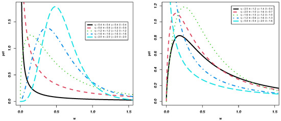
Figure 1. The pdf for the TIIEHL-PLo model.

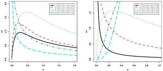
Figure 2. The hrf for the TIIEHL-PLo model.

3. Basic Statistical Properties

The structural characteristics of the TIIEHL-PLo model are described in this part, including the QF, the nth raw moments, mean, variance, skewness, kurtosis, the moment-generating function, many graphical and numerical results of moments, and order statistics.

3.1. Quantile Function and MacGillivray’s Skewness

Suppose that the random variable W ∼ TIIEHL-PLo($\mathsf{\Theta })$, then its QF is provided in Equation (10) as

$$w={\left\{{\left[1-{\left(\frac{1-{\left(1-p\right)}^{\frac{1}{\delta }}}{1+{\left(1-p\right)}^{\frac{1}{\delta }}}\right)}^{\frac{1}{\gamma }}\right]}^{\frac{-1}{\eta }}-1\right\}}^{\frac{1}{\theta }},$$

(10)

where $p\sim uniform(0,1)$. By putting $p=0.5$ in Equation (10), we obtain the median (M) of the TIIEHL-PLo model as below

$$M={\left\{{\left[1-{\left(\frac{1-{\left(0.5\right)}^{\frac{1}{\delta }}}{1+{\left(0.5\right)}^{\frac{1}{\delta }}}\right)}^{\frac{1}{\gamma }}\right]}^{\frac{-1}{\eta }}-1\right\}}^{\frac{1}{\theta }}.$$

The MacGillivray’s skewness ($MGS$) [29] is derived from the following expression.

$$MGS=\frac{w_p+w_{1-p}-2w_{0.5}}{w_p-w_{1-p}},0<p<1.$$

3.2. Moments

Suppose that W ∼ TIIEHL-PLo($\mathsf{\Theta }$) for $w\in \left(0,\infty \right)$ and $\mathsf{\Theta }>0$, then the nth raw moments can be computed from the formula below

$$\begin{array}{c}{\mu }_n^{\prime }={\int }_0^{\infty }{w}^{n}f\left(w;\mathsf{\Theta }\right)dw\hfill \\ =2\delta \gamma \theta \eta {\int }_0^{\infty }\frac{w^{n+\theta -1}{\left(1+w^{\theta }\right)}^{-\eta -1}{\left[1-{\left(1+w^{\theta }\right)}^{-\eta }\right]}^{\gamma -1}{\left(1-{\left[1-{\left(1+w^{\theta }\right)}^{-\eta }\right]}^{\gamma }\right)}^{\delta -1}}{{\left(1+{\left[1-{\left(1+w^{\theta }\right)}^{-\eta }\right]}^{\gamma }\right)}^{\delta +1}}dw.\hfill \end{array}$$

(11)

By using the next two binomial expansions

$${\left(1+w\right)}^{-\delta -1}=\sum _{i=0}^{\infty }{\left(-1\right)}^i\left(\begin{array}{c}\delta +i\\ i\end{array}\right)w^i,$$

(12)

and

$${\left(1-w\right)}^{\delta -1}=\sum _{j=0}^{\delta -1}{\left(-1\right)}^j\left(\begin{array}{c}\delta -1\\ j\end{array}\right)w^j.$$

(13)

By inserting (12) and (13) in (11), we then obtain

$${\mu }_n^{\prime }=2\delta \gamma \theta \eta \sum _{i=0}^{\infty }\sum _{j=0}^{\delta -1}{\left(-1\right)}^{i+j}\left(\begin{array}{c}\delta +i\\ i\end{array}\right)\left(\begin{array}{c}\delta -1\\ j\end{array}\right){\int }_0^{\infty }{w}^{n+\theta -1}{\left(1+w^{\theta }\right)}^{-\eta -1}{\left[1-{\left(1+w^{\theta }\right)}^{-\eta }\right]}^{\gamma \left(i+j+1\right)-1}dw.$$

Again, using expansion (13) in the last formula, then

$${\mu }_n^{\prime }=\theta \sum _{i=0}^{\infty }\sum _{j=0}^{\delta -1}\sum _{k=0}^{\gamma \left(i+j+1\right)-1}{\mathsf{\Xi }}_{i,j,k}{\int }_0^{\infty }{w}^{n+\theta -1}{\left(1+w^{\theta }\right)}^{-\eta \left(k+1\right)-1}dw,$$

where ${\mathsf{\Xi }}_{i,j,k}=2\delta \gamma \eta {\left(-1\right)}^{i+j+k}\left(\begin{array}{c}\delta +i\\ i\end{array}\right)\left(\begin{array}{c}\delta -1\\ j\end{array}\right)\left(\begin{array}{c}\gamma \left(i+j+1\right)-1\\ k\end{array}\right).$

Let $y=w^{\theta }$, then

$${\mu }_n^{\prime }=\sum _{i=0}^{\infty }\sum _{j=0}^{\delta -1}\sum _{k=0}^{\gamma \left(i+j+1\right)-1}{\mathsf{\Xi }}_{i,j,k}{\int }_0^{\infty }{y}^{\frac{n}{\theta }}{\left(1+y\right)}^{-\eta \left(k+1\right)-1}dy.$$

By using the beta prime function $B\left(\alpha ,\beta \right)={\int }_0^{\infty }{y}^{\alpha -1}{\left(1+y\right)}^{-\alpha -\beta }dy.$ Then, the nth raw moments of the TIIEHL-PLo model is provided via

$${\mu }_n^{\prime }=\sum _{i=0}^{\infty }\sum _{j=0}^{\delta -1}\sum _{k=0}^{\gamma \left(i+j+1\right)-1}{\mathsf{\Xi }}_{i,j,k}B\left[\frac{n}{\theta }+1,\eta \left(k+1\right)-\frac{n}{\theta }\right],\frac{n}{\theta }<\eta \left(k+1\right).$$

(14)

To obtain the first four raw moments, we put n = 1, 2, 3, and 4 in (14), respectively, as

$${\mu }_1^{\prime }=\sum _{i=0}^{\infty }\sum _{j=0}^{\delta -1}\sum _{k=0}^{\gamma \left(i+j+1\right)-1}{\mathsf{\Xi }}_{i,j,k}B\left[\frac{1}{\theta }+1,\eta \left(k+1\right)-\frac{1}{\theta }\right],\frac{1}{\theta }<\eta \left(k+1\right),$$

$${\mu }_2^{\prime }=\sum _{i=0}^{\infty }\sum _{j=0}^{\delta -1}\sum _{k=0}^{\gamma \left(i+j+1\right)-1}{\mathsf{\Xi }}_{i,j,k}B\left[\frac{2}{\theta }+1,\eta \left(k+1\right)-\frac{2}{\theta }\right],\frac{2}{\theta }<\eta \left(k+1\right),$$

$${\mu }_3^{\prime }=\sum _{i=0}^{\infty }\sum _{j=0}^{\delta -1}\sum _{k=0}^{\gamma \left(i+j+1\right)-1}{\mathsf{\Xi }}_{i,j,k}B\left[\frac{3}{\theta }+1,\eta \left(k+1\right)-\frac{3}{\theta }\right],\frac{3}{\theta }<\eta \left(k+1\right),$$

and

$${\mu }_4^{\prime }=\sum _{i=0}^{\infty }\sum _{j=0}^{\delta -1}\sum _{k=0}^{\gamma \left(i+j+1\right)-1}{\mathsf{\Xi }}_{i,j,k}B\left[\frac{4}{\theta }+1,\eta \left(k+1\right)-\frac{4}{\theta }\right],\frac{4}{\theta }<\eta \left(k+1\right).$$

The $E\left(W\right)$, var, S and K are computed, respectively, from the following formulas $E\left(W\right)={\mu }_1^{\prime },$ $var={\mu }_2^{\prime }-{\left({\mu }_1^{\prime }\right)}^2,$ $S=\frac{{\left({\mu }_3^{\prime }-3{\mu }_1^{\prime }{\mu }_2^{\prime }+2{\left({\mu }_1^{\prime }\right)}^3\right)}^2}{{\left({\mu }_2^{\prime }-{\left({\mu }_1^{\prime }\right)}^2\right)}^3}$ and $K=\frac{{\mu }_4^{\prime }-4{\mu }_3^{\prime }{\mu }_1^{\prime }+6{\mu }_2^{\prime }{\left({\mu }_1^{\prime }\right)}^2-3{\left({\mu }_1^{\prime }\right)}^4}{{\left({\mu }_2^{\prime }-{\left({\mu }_1^{\prime }\right)}^2\right)}^2}$.

The moment-generating function for the TIIEHL-PLo model is

$$\begin{array}{c}{M}_w\left(t\right)=E\left(e^{tW}\right)=\underset{0}{\overset{\infty }{\int }}{e}^{tw}f\left(w;\mathsf{\Theta }\right)dw={\displaystyle \sum _{n=0}^{\infty }}\frac{t^n}{n!}{\mu }_n^{\prime }\hfill \\ ={\displaystyle \sum _{n=0}^{\infty }}{\displaystyle \sum _{i=0}^{\infty }}{\displaystyle \sum _{j=0}^{\delta -1}}{\displaystyle \sum _{k=0}^{\gamma \left(i+j+1\right)-1}}\frac{t^n{\mathsf{\Xi }}_{i,j,k}}{n!}B\left[\frac{n}{\theta }+1,\eta \left(k+1\right)-\frac{n}{\theta }\right].\hfill \end{array}$$

Table 1 shows some numerical values of ${\mu }_1^{\prime }$, ${\mu }_2^{\prime }$, ${\mu }_3^{\prime }$, ${\mu }_4^{\prime }$, var, S, K, and CV for the TIIEHL-PLo model using different values of $\mathsf{\Theta }$.

Table 1. Some numerical values of ${\mu }_1^{\prime }$, ${\mu }_2^{\prime }$, ${\mu }_3^{\prime }$, ${\mu }_4^{\prime }$, var, S, K, and CV.

$\mathit{\delta }$	$\mathit{\gamma }$	$\mathit{\eta }$	$\mathit{\theta }$	${\mathit{\mu }}_1^{\prime }$	${\mathit{\mu }}_2^{\prime }$	${\mathit{\mu }}_3^{\prime }$	${\mathit{\mu }}_4^{\prime }$	var	S	K	CV
2	2	2	2	0.6	0.435	0.383	0.415	0.076	1.479	8.287	0.459
			2.5	0.654	0.484	0.404	0.382	0.056	1.062	5.82	0.362
			3	0.696	0.528	0.435	0.391	0.044	0.812	4.806	0.3
		2.5	2	0.524	0.327	0.241	0.211	0.053	1.245	6.503	0.438
			2.5	0.587	0.387	0.284	0.232	0.042	0.891	4.92	0.348
			3	0.637	0.439	0.327	0.262	0.034	0.671	4.234	0.289
		3	2	0.471	0.262	0.17	0.128	0.04	1.109	5.673	0.425
			2.5	0.54	0.325	0.216	0.158	0.033	0.788	4.469	0.338
			3	0.594	0.38	0.262	0.193	0.028	0.584	3.937	0.282
	3	2	2	0.755	0.657	0.664	0.799	0.087	1.479	8.493	0.39
			2.5	0.79	0.682	0.647	0.679	0.059	1.101	6.127	0.307
			3	0.816	0.709	0.657	0.65	0.043	0.877	5.123	0.254
		2.5	2	0.654	0.486	0.41	0.397	0.058	1.223	6.569	0.367
			2.5	0.705	0.539	0.447	0.403	0.042	0.91	5.111	0.29
			3	0.743	0.584	0.486	0.428	0.032	0.716	4.454	0.241
		3	2	0.585	0.385	0.285	0.237	0.043	1.074	5.682	0.353
			2.5	0.645	0.449	0.337	0.272	0.033	0.794	4.605	0.28
			3	0.691	0.503	0.385	0.311	0.026	0.617	4.11	0.232
4	2	2	2	0.454	0.235	0.137	0.089	0.029	0.742	4.234	0.378
			2.5	0.525	0.301	0.187	0.125	0.025	0.482	3.638	0.303
			3	0.581	0.359	0.235	0.162	0.022	0.311	3.392	0.254
		2.5	2	0.4	0.182	0.093	0.052	0.022	0.661	3.948	0.369
			2.5	0.476	0.246	0.137	0.082	0.02	0.416	3.47	0.297
			3	0.535	0.304	0.182	0.115	0.018	0.252	3.282	0.249
		3	2	0.362	0.149	0.068	0.034	0.017	0.61	3.784	0.363
			2.5	0.439	0.209	0.107	0.059	0.017	0.373	3.374	0.293
			3	0.501	0.266	0.149	0.087	0.015	0.213	3.219	0.245
	3	2	2	0.599	0.393	0.28	0.217	0.034	0.679	4.184	0.308
			2.5	0.659	0.46	0.34	0.265	0.026	0.46	3.696	0.246
			3	0.703	0.515	0.393	0.311	0.021	0.316	3.485	0.206
		2.5	2	0.525	0.3	0.186	0.124	0.024	0.584	3.883	0.297
			2.5	0.593	0.372	0.246	0.17	0.02	0.379	3.513	0.238
			3	0.645	0.432	0.3	0.216	0.017	0.243	3.361	0.199
		3	2	0.474	0.243	0.134	0.08	0.019	0.523	3.713	0.291
			2.5	0.546	0.315	0.19	0.12	0.016	0.326	3.411	0.233
			3	0.602	0.376	0.243	0.163	0.014	0.195	3.293	0.195

3.3. Order Statistics

Suppose that $W_1,W_2,\dots ,W_n$ is a random sample from the TIIEHL-PLo model with order statistics $W_{\left(1\right)},W_{\left(2\right)},\dots ,W_{\left(n\right)}$. The pdf of $W_{\left(s\right)}$ of order statistics can be computed from the next formula

$$f_{W_{\left(s\right)}}(w;\mathsf{\Theta })=\frac{n!}{(s-1)!(n-s)!}{F}^{(s-1)}(w;\mathsf{\Theta })f(w;\mathsf{\Theta }){(1-F(w;\mathsf{\Theta }))}^{(n-s)}.$$

(15)

By inserting (8) and (9) in (15), we obtain the pdf of $W_{\left(s\right)}$ of order statistics for the TIIEHL-PLo model as

$$f_{W_{\left(s\right)}}(w;\mathsf{\Theta })=\frac{2\delta \gamma \theta \eta w^{\theta -1}n!}{(s-1)!(n-s)!}{\left(1-{\left[\frac{1-{\left[\mathsf{\Psi }\right]}^{\gamma }}{1+{\left[\mathsf{\Psi }\right]}^{\gamma }}\right]}^{\delta }\right)}^{s-1}\frac{{\left(1+w^{\theta }\right)}^{-\eta -1}{\left[\mathsf{\Psi }\right]}^{\gamma -1}{\left(1-{\left[\mathsf{\Psi }\right]}^{\gamma }\right)}^{\delta (n-s+1)-1}}{{\left(1+{\left[\mathsf{\Psi }\right]}^{\gamma }\right)}^{\delta (n-s+1)+1}}.$$

(16)

where $1-{\left(1+w^{\theta }\right)}^{-\eta }=\mathsf{\Psi }$. By putting s = 1 and n, we obtain the first and largest order statistics as below

$$f_{W_{\left(1\right)}}\left(w\right)=2n\delta \gamma \theta \eta w^{\theta -1}\frac{{\left(1+w^{\theta }\right)}^{-\eta -1}{\left[\mathsf{\Psi }\right]}^{\gamma -1}{\left(1-{\left[\mathsf{\Psi }\right]}^{\gamma }\right)}^{n\delta -1}}{{\left(1+{\left[\mathsf{\Psi }\right]}^{\gamma }\right)}^{n\delta +1}},$$

and

$$f_{W_{\left(n\right)}}\left(w\right)=2n\delta \gamma \theta \eta w^{\theta -1}{\left(1-{\left[\frac{1-{\left[\mathsf{\Psi }\right]}^{\gamma }}{1+{\left[\mathsf{\Psi }\right]}^{\gamma }}\right]}^{\delta }\right)}^{n-1}\frac{{\left(1+w^{\theta }\right)}^{-\eta -1}{\left[\mathsf{\Psi }\right]}^{\gamma -1}{\left(1-{\left[\mathsf{\Psi }\right]}^{\gamma }\right)}^{\delta -1}}{{\left(1+{\left[\mathsf{\Psi }\right]}^{\gamma }\right)}^{\delta +1}}.$$

4. Six Different Approaches of Estimation

The parameters of the TIIEHL-PLo distribution are estimated in this section using the ML, MPS, AD, CVM, LS, and WLS approaches of estimation.

4.1. Maximum Likelihood Approach of Estimation

Let $(w_1,w_2,\dots ,w_n)$ be a random sample from the TIIEHL-PLo model, then the ML estimation (MLE) function $L\left(\mathsf{\Theta }\right)$ can be supplied as below:

$$\begin{array}{cc}\hfill L\left(\mathsf{\Theta }\right)& =\prod _{i=1}^{n}f(w_i;\mathsf{\Theta })\hfill \\ \hfill & ={\left(2\delta \gamma \theta \eta \right)}^n\prod _{i=1}^n\frac{w_i^{\theta -1}{\left(1+w_i^{\theta }\right)}^{-\eta -1}{\left[1-{\left(1+w_i^{\theta }\right)}^{-\eta }\right]}^{\gamma -1}{\left(1-{\left[1-{\left(1+w_i^{\theta }\right)}^{-\eta }\right]}^{\gamma }\right)}^{\delta -1}}{{\left(1+{\left[1-{\left(1+w_i^{\theta }\right)}^{-\eta }\right]}^{\gamma }\right)}^{\delta +1}},\hfill \end{array}$$

(17)

and the natural log-likelihood function of the TIIEHL-PLo model is provided via

$$\begin{array}{cc}\hfill ln\left(L\right(\mathsf{\Theta }\left)\right)=& n\left[ln\left(2\right)+ln\left(\delta \right)+ln\left(\gamma \right)+ln\left(\theta \right)+ln\left(\eta \right)\right]-(\eta +1)\sum _{i=1}^{n}ln\left(1+w_i^{\theta }\right)+\hfill \\ & (\gamma -1)\sum _{i=1}^{n}ln\left[1-{\left(1+w_i^{\theta }\right)}^{-\eta }\right]+(\delta -1)\sum _{i=1}^{n}ln\left(1-{\left[1-{\left(1+w_i^{\theta }\right)}^{-\eta }\right]}^{\gamma }\right)-\hfill \\ & (\delta +1)\sum _{i=1}^{n}ln\left(1+{\left[1-{\left(1+w_i^{\theta }\right)}^{-\eta }\right]}^{\gamma }\right)+(\theta -1)\sum _{i=1}^{n}ln\left(w_i\right).\hfill \end{array}$$

(18)

With regard to $\mathsf{\Theta }$, the natural log-likelihood function’s first derivatives are provided below

$$\begin{array}{cc}\hfill \frac{\partial ln\left(L\right(\mathsf{\Theta }\left)\right)}{\partial \theta }=& \frac{n}{\theta }-(\eta +1)\sum _{i=1}^n\frac{w_i^{\theta }ln\left(w_i\right)}{1+w_i^{\theta }}+(\gamma -1)\eta \sum _{i=1}^n\frac{w_i^{\theta }ln\left(w_i\right){\left(1+w_i^{\theta }\right)}^{-\eta -1}}{1-{\left(1+w_i^{\theta }\right)}^{-\eta }}-\hfill \\ & (\delta -1)\eta \gamma \sum _{i=1}^n\frac{w_i^{\theta }ln\left(w_i\right){\left(1+w_i^{\theta }\right)}^{-\eta -1}{\left[1-{\left(1+w_i^{\theta }\right)}^{-\eta }\right]}^{\gamma -1}}{1-{\left[1-{\left(1+w_i^{\theta }\right)}^{-\eta }\right]}^{\gamma }}-\hfill \\ & (\delta +1)\eta \gamma \sum _{i=1}^n\frac{w_i^{\theta }ln\left(w_i\right){\left(1+w_i^{\theta }\right)}^{-\eta -1}{\left[1-{\left(1+w_i^{\theta }\right)}^{-\eta }\right]}^{\gamma -1}}{1+{\left[1-{\left(1+w_i^{\theta }\right)}^{-\eta }\right]}^{\gamma }}+\sum _{i=1}^{n}ln\left(w_i\right),\hfill \end{array}$$

(19)

$$\begin{array}{cc}\hfill \frac{\partial ln\left(L\right(\mathsf{\Theta }\left)\right)}{\partial \gamma }=& \frac{n}{\gamma }+\sum _{i=1}^{n}ln\left[1-{\left(1+w_i^{\theta }\right)}^{-\eta }\right]-\hfill \\ & (\delta -1)\sum _{i=1}^n\frac{ln\left[1-{\left(1+w_i^{\theta }\right)}^{-\eta }\right]{\left[1-{\left(1+w_i^{\theta }\right)}^{-\eta }\right]}^{\gamma }}{1-{\left[1-{\left(1+w_i^{\theta }\right)}^{-\eta }\right]}^{\gamma }}-\hfill \\ & (\delta +1)\sum _{i=1}^n\frac{ln\left[1-{\left(1+w_i^{\theta }\right)}^{-\eta }\right]{\left[1-{\left(1+w_i^{\theta }\right)}^{-\eta }\right]}^{\gamma }}{1+{\left[1-{\left(1+w_i^{\theta }\right)}^{-\eta }\right]}^{\gamma }},\hfill \end{array}$$

(20)

$$\begin{array}{cc}\hfill \frac{\partial ln\left(L\right(\mathsf{\Theta }\left)\right)}{\partial \eta }=& \frac{n}{\eta }-\sum _{i=1}^{n}ln\left(1+w_i^{\theta }\right)+(\gamma -1)\sum _{i=1}^n\frac{ln\left(1+w_i^{\theta }\right){\left(1+w_i^{\theta }\right)}^{-\eta }}{1-{\left(1+w_i^{\theta }\right)}^{-\eta }}-\hfill \\ & (\delta -1)\gamma \sum _{i=1}^n\frac{ln\left(1+w_i^{\theta }\right){\left(1+w_i^{\theta }\right)}^{-\eta }{\left[1-{\left(1+w_i^{\theta }\right)}^{-\eta }\right]}^{\gamma -1}}{1-{\left[1-{\left(1+w_i^{\theta }\right)}^{-\eta }\right]}^{\gamma }}-\hfill \\ & (\delta +1)\gamma \sum _{i=1}^n\frac{ln\left(1+w_i^{\theta }\right){\left(1+w_i^{\theta }\right)}^{-\eta }{\left[1-{\left(1+w_i^{\theta }\right)}^{-\eta }\right]}^{\gamma -1}}{1+{\left[1-{\left(1+w_i^{\theta }\right)}^{-\eta }\right]}^{\gamma }},\hfill \end{array}$$

(21)

$$\begin{array}{c}\\ \hfill \frac{\partial ln\left(L\right(\mathsf{\Theta }\left)\right)}{\partial \delta }=& \frac{n}{\delta }+\sum _{i=1}^{n}ln\left(1-{\left[1-{\left(1+w_i^{\theta }\right)}^{-\eta }\right]}^{\gamma }\right)-\hfill \\ & \sum _{i=1}^{n}ln\left(1+{\left[1-{\left(1+w_i^{\theta }\right)}^{-\eta }\right]}^{\gamma }\right),\hfill \end{array}$$

(22)

Numerical approaches are utilized to provide solutions to the Equations (19)–(22), which have no analytic closed form when equating to zero. Since the aforementioned equations are nonlinear, the Newton–Raphson approach in R is employed to estimate the model parameters.

4.2. Maximum Product Spacing Approach of Estimation

A good substitute for the greatest likelihood approach is the maximum product spacing method, which approximates the Kullback–Leibler information measure. Let us now suppose that the data are ordered in an increasing manner. Then, the maximum product spacing for the TIIEHL-PLo distribution is given as follows

$$Gs\left(\mathsf{\Theta }\right|data)={\left(\prod _{i=1}^{n+1}{D}_l(w_i,\mathsf{\Theta })\right)}^{\frac{1}{n+1}},$$

(23)

where $D_l(w_i,\mathsf{\Theta })=F(w_i;\mathsf{\Theta })-F(w_{i-1};\mathsf{\Theta })$, $i=1,2,3,\dots ,n+1$.

Similarly, one can also choose to maximize the function

$$H\left(\mathsf{\Theta }\right)=\frac{1}{n+1}\sum _{i=1}^{n+1}ln{D}_i\left(\mathsf{\Theta }\right).$$

(24)

By taking the first derivative of the function $H\left(\mathsf{\Theta }\right)$ with respect to $\gamma$, $\delta$, $\eta$, and $\theta$, and solving the resulting nonlinear equations, at $\frac{\partial H\left(\mathsf{\Theta }\right)}{\partial \gamma }$ = 0, $\frac{\partial H\left(\mathsf{\Theta }\right)}{\partial \delta }$ = 0, $\frac{\partial H\left(\mathsf{\Theta }\right)}{\partial \eta }$ = 0, and $\frac{\partial H\left(\mathsf{\Theta }\right)}{\partial \theta }$ = 0, where $\mathsf{\Theta }=(\gamma ,\delta ,\eta ,\theta )$, we obtain the value of the parameter estimates.

4.3. Anderson and Darling Approach of Estimation

The function regarding to the model parameters $\mathsf{\Theta }$ is minimized to obtain the AD estimates, which are written as

$$\begin{array}{c}\hfill AD\left(\mathsf{\Theta }\right)=-n-\frac{1}{n}\sum _{k=1}^n(2k-1)(lnF(w_k,\mathsf{\Theta })+ln\overline{F}(w_{n+1-k},\mathsf{\Theta })),\end{array}$$

where $\overline{F}(x,\mathsf{\Theta })=1-F(x,\mathsf{\Theta })$.

4.4. Cramer-von-Mises Approach of Estimation

Another significant estimating approach commented upon in Ref. [30] is the CVM. By minimizing the function $C(w,\mathsf{\Theta })$ with respect to the unknown parameters $\mathsf{\Theta }$, the parameters in the CVM estimation technique can be estimated.

$$\begin{array}{c}\hfill C(w,\mathsf{\Theta })=\frac{1}{12}+\sum _{k=1}^n{\left[F(w_k,\mathsf{\Theta })-\frac{2k-1}{2n}\right]}^2\end{array}$$

$$\begin{array}{c}\hfill =\frac{1}{12}+\sum _{k=1}^n{\left[1-{\left[\frac{1-{\left[1-{\left(1+w_k^{\theta }\right)}^{-\eta }\right]}^{\gamma }}{1+{\left[1-{\left(1+w_k\theta \right)}^{-\eta }\right]}^{\gamma }}\right]}^{\delta }-\frac{2k-1}{2n}\right]}^2.\end{array}$$

4.5. Least Square and Weighted Least Square Approaches of Estimation

To estimate the parameters of the beta model, Ref. [31] offers LS and WLS techniques of estimation. The LS function $LS\left(\mathsf{\Theta }\right)$ regarding the unknown parameters can be minimized in the LS estimation (LSE) approach to provide the estimates of the parameters $\mathsf{\Theta }$ of the proposed model, where

$$\begin{array}{c}\hfill LS\left(\mathsf{\Theta }\right)=\sum _{k=1}^n{\left[F(w_k,\mathsf{\Theta })-\frac{k}{n+1}\right]}^2\end{array}$$

$$\begin{array}{c}\hfill =\sum _{k=1}^n{\left[1-{\left[\frac{1-{\left[1-{\left(1+w_k^{\theta }\right)}^{-\eta }\right]}^{\gamma }}{1+{\left[1-{\left(1+w_k\theta \right)}^{-\eta }\right]}^{\gamma }}\right]}^{\delta }-\frac{k}{n+1}\right]}^2.\end{array}$$

Similarly to this, the WLS function $WLS\left(\mathsf{\Theta }\right)$ was minimized to compute the WLS estimation (WLSE) of the unknown parameters:

$$\begin{array}{c}\hfill WLS\left(\mathsf{\Theta }\right)=\sum _{k=1}^n\frac{{(n+1)}^2(n+2)}{k(n-k+1)}{\left[F(w_k,\mathsf{\Theta })-\frac{k}{n+1}\right]}^2\end{array}$$

$$\begin{array}{c}\hfill =\sum _{k=1}^n\frac{{(n+1)}^2(n+2)}{k(n-k+1)}{\left[1-{\left[\frac{1-{\left[1-{\left(1+w_k^{\theta }\right)}^{-\eta }\right]}^{\gamma }}{1+{\left[1-{\left(1+w_k\theta \right)}^{-\eta }\right]}^{\gamma }}\right]}^{\delta }-\frac{k}{n+1}\right]}^2.\end{array}$$

5. Simulation

The ML, AD, CVM, MPS, LS, and WLS techniques are combined with a Monte Carlo simulation to estimate the parameters in this section. Using the R package and the following:

• Simulation techniques for various parameters $\left(\mathsf{\Theta }\right)$ with varied actual values of the parameters, datum w is distributed as a TIIEHL-PLo distribution: Using the R package and the following:
  In Table 2, $\eta =0.85,\theta =0.6,\delta =1.2$ and $\gamma =$ 0.7, and 1.8;
  Table 2. Different estimations for $\eta =0.85,\theta =0.6,\delta =1.2$.

  			MLE		LS		WLS		MPS		CVM		AD
  $\mathbf{\gamma }$	N		Bias	MSE	Bias	MSE	Bias	MSE	Bias	MSE	Bias	MSE	Bias	MSE
  0.7	50	$\eta$	0.4280	0.7539	0.0622	0.0202	0.1751	0.0561	0.4285	0.2607	0.0923	0.0249	0.1623	0.0448
  		$\theta$	0.0990	0.1072	0.1190	0.0422	0.1108	0.0627	0.0985	0.1286	0.1365	0.0438	0.1295	0.0614
  		$\gamma$	0.3489	0.4889	0.0078	0.0376	0.1258	0.0992	0.3501	0.2757	0.0241	0.0406	0.0962	0.0781
  		$\delta$	−0.0008	0.1380	0.0068	0.0385	0.0246	0.0724	−0.0075	0.1089	0.0230	0.0416	0.0230	0.0625
  	100	$\eta$	0.5073	0.5146	0.0617	0.0176	0.1678	0.0399	0.4051	0.2427	0.0811	0.0191	0.1515	0.0350
  		$\theta$	−0.0574	0.0439	0.0625	0.0173	0.0368	0.0242	−0.0573	0.0469	0.0721	0.0177	0.0498	0.0236
  		$\gamma$	0.3451	0.3547	0.0064	0.0280	0.1205	0.0629	0.3451	0.2424	0.0235	0.0281	0.1201	0.0545
  		$\delta$	0.0228	0.0901	0.0052	0.0239	0.0204	0.0399	0.0062	0.0721	0.0220	0.0256	0.0401	0.0373
  	150	$\eta$	0.4173	0.5023	0.0605	0.0114	0.1577	0.0343	0.3954	0.2351	0.0777	0.0134	0.1223	0.0183
  		$\theta$	−0.0498	0.0325	0.0608	0.0168	0.0011	0.0130	−0.0398	0.0324	0.0698	0.0169	0.0514	0.0140
  		$\gamma$	0.4009	0.3238	0.0050	0.0218	0.1205	0.0436	0.3291	0.2334	0.0219	0.0244	0.0788	0.0245
  		$\delta$	0.0213	0.0790	0.0042	0.0194	0.0206	0.0273	0.0053	0.0566	0.0210	0.0208	0.0352	0.0213
  1.8	50	$\eta$	−0.1993	0.5622	0.0126	0.0210	0.0347	0.0571	−0.1985	0.2099	0.0235	0.0244	−0.0050	0.0386
  		$\theta$	0.3262	0.1620	0.0296	0.0155	0.0646	0.0257	0.3264	0.1883	0.0506	0.0156	0.0613	0.0262
  		$\gamma$	−0.1639	0.6559	−0.0198	0.0335	−0.0286	0.0993	−0.1640	0.4649	−0.0041	0.0312	−0.0192	0.0906
  		$\delta$	0.2018	0.8703	0.0010	0.0714	0.0330	0.2234	0.2009	0.5129	0.0110	0.0812	0.0636	0.1914
  	100	$\eta$	−0.1804	0.2264	0.0126	0.0155	0.0318	0.0302	−0.1807	0.1348	0.0229	0.0171	0.0154	0.0313
  		$\theta$	0.2439	0.0739	0.0200	0.0072	0.0404	0.0120	0.2441	0.0952	0.0309	0.0076	0.0608	0.0164
  		$\gamma$	−0.1591	0.3190	−0.0154	0.0245	−0.0218	0.0580	−0.1592	0.3447	−0.0038	0.0246	−0.0336	0.0794
  		$\delta$	0.1175	0.3940	−0.0010	0.0654	0.0029	0.1266	0.1173	0.3085	−0.0042	0.0734	0.0106	0.1456
  	150	$\eta$	−0.1507	0.2133	0.0123	0.0146	0.0261	0.0256	−0.1509	0.1000	0.0219	0.0152	0.0242	0.0279
  		$\theta$	0.1755	0.0456	0.0166	0.0055	0.0401	0.0113	0.1755	0.0571	0.0258	0.0059	0.0530	0.0125
  		$\gamma$	−0.1279	0.3049	−0.0092	0.0211	−0.0209	0.0497	−0.1280	0.2543	−0.0035	0.0208	−0.0285	0.0603
  		$\delta$	0.1087	0.3840	0.0002	0.0649	−0.0019	0.0909	0.1089	0.2515	−0.0027	0.0673	−0.0059	0.1109

  In Table 3, $\theta =2,\gamma =1.8,\delta =1.2$ and $\eta =$ 0.85 and 2;
  Table 3. Different estimations for $\theta =2,\gamma =1.8,\delta =1.2$.

  			MLE		LS		WLS		MPS		CVM		AD
  $\mathbf{\eta }$	n		Bias	MSE	Bias	MSE	Bias	MSE	Bias	MSE	Bias	MSE	Bias	MSE
  0.85	50	$\eta$	−0.1158	0.7176	0.0087	0.0276	0.0595	0.0638	−0.1147	0.2391	0.0283	0.0333	0.0232	0.0591
  		$\theta$	0.1581	0.5360	0.0052	0.0682	0.0220	0.0945	0.1583	0.5926	0.0129	0.0709	0.0414	0.1421
  		$\gamma$	−0.1195	0.6751	−0.0015	0.0285	−0.0037	0.0488	−0.1194	0.3125	0.0259	0.0297	−0.0106	0.0722
  		$\delta$	0.2172	0.9925	0.0480	0.1066	0.0381	0.2152	0.2162	0.5175	0.0650	0.1208	0.0718	0.2267
  	100	$\eta$	−0.1076	0.4903	0.0067	0.0188	0.0335	0.0318	−0.1078	0.1567	0.0236	0.0190	0.0346	0.0310
  		$\theta$	0.1354	0.3672	0.0052	0.0331	0.0116	0.0447	0.1356	0.3558	0.0125	0.0342	0.0226	0.0595
  		$\gamma$	−0.1194	0.4995	−0.0015	0.0144	−0.0035	0.0230	−0.1196	0.2306	0.0041	0.0133	−0.0089	0.0306
  		$\delta$	0.1257	0.5805	−0.0157	0.0606	0.0165	0.1039	0.1255	0.3126	0.0053	0.0596	0.0135	0.1189
  	150	$\eta$	−0.0927	0.3670	0.0061	0.0133	0.0327	0.0306	−0.0930	0.1169	0.0238	0.0159	0.0331	0.0314
  		$\theta$	0.1061	0.2978	−0.0005	0.0224	0.0102	0.0398	0.1061	0.2503	0.0065	0.0248	0.0199	0.0518
  		$\gamma$	−0.0981	0.4457	0.0012	0.0097	−0.0034	0.0201	−0.0982	0.1726	0.0041	0.0101	−0.0050	0.0271
  		$\delta$	0.1078	0.4370	0.0148	0.0479	−0.0135	0.0773	0.1081	0.2468	0.0042	0.0554	0.0125	0.1080
  2	50	$\eta$	−0.0369	2.5221	−0.0068	0.1066	0.0114	0.3297	−0.0363	0.5137	0.0058	0.1083	0.0085	0.3407
  		$\theta$	0.1304	0.9183	0.0100	0.0510	0.0363	0.1301	0.1302	0.5371	0.0265	0.0533	0.0477	0.1415
  		$\gamma$	−0.0608	1.8920	−0.0055	0.0692	0.0154	0.2606	−0.0601	0.4946	0.0088	0.0687	0.0133	0.2614
  		$\delta$	−0.0278	0.2960	0.0077	0.0264	0.0064	0.0438	−0.0283	0.0700	0.0282	0.0302	0.0149	0.0426
  	100	$\eta$	−0.0301	1.8807	0.0061	0.1023	−0.0037	0.1128	−0.0300	0.2962	0.0042	0.1025	0.0073	0.2314
  		$\theta$	0.0616	0.5196	0.0100	0.0461	0.0152	0.0494	0.0615	0.2241	0.0197	0.0516	0.0146	0.0704
  		$\gamma$	−0.0330	1.4274	0.0055	0.0611	−0.0047	0.0900	−0.0328	0.2915	0.0069	0.0609	0.0132	0.1928
  		$\delta$	−0.0131	0.1896	0.0035	0.0257	0.0032	0.0163	−0.0131	0.0344	0.0101	0.0289	−0.0011	0.0239
  	150	$\eta$	−0.0362	1.1643	−0.0001	0.0304	0.0037	0.1040	−0.0301	0.2080	0.0038	0.0271	−0.0034	0.0815
  		$\theta$	0.0562	0.3912	0.0020	0.0153	0.0120	0.0455	0.0563	0.1433	0.0074	0.0147	0.0137	0.0360
  		$\gamma$	−0.0445	0.8100	−0.0001	0.0200	0.0038	0.0886	−0.0304	0.2089	0.0040	0.0174	−0.0033	0.0652
  		$\delta$	−0.0085	0.1514	0.0021	0.0080	0.0014	0.0158	−0.0082	0.0228	0.0084	0.0082	0.0058	0.0103

  In Table 4, $\eta =3,\gamma =3,\delta =2$ and $\theta =$ 1.2 and 3;
  Table 4. Different estimations for $\eta =3,\gamma =3,\delta =2$.

  			MLE		LS		WLS		MPS		CVM		AD
  $\mathbf{\theta }$	n		Bias	MSE	Bias	MSE	Bias	MSE	Bias	MSE	Bias	MSE	Bias	MSE
  1.2	50	$\eta$	−0.0334	1.0185	0.0070	0.1627	−0.0056	0.1478	−0.0330	0.5284	0.0233	0.1741	0.0018	0.4672
  		$\theta$	0.0557	0.2945	0.0045	0.0196	0.0137	0.0176	0.0556	0.0920	0.0290	0.0216	0.0515	0.0429
  		$\gamma$	−0.0531	0.9668	−0.0073	0.0806	−0.0128	0.0780	−0.0527	0.5641	0.0037	0.0868	−0.0244	0.3677
  		$\delta$	−0.0123	0.2988	0.0049	0.0793	0.0187	0.0701	−0.0127	0.1462	0.0190	0.0845	0.0293	0.1717
  	100	$\eta$	−0.0118	0.8033	−0.0051	0.0462	0.0043	0.0824	−0.0117	0.2774	0.0021	0.0472	0.0016	0.1072
  		$\theta$	0.0146	0.0913	−0.0014	0.0082	0.0036	0.0076	0.0146	0.0274	0.0107	0.0086	0.0080	0.0090
  		$\gamma$	−0.0212	0.6897	−0.0047	0.0151	−0.0066	0.0455	−0.0210	0.2920	−0.0048	0.0153	−0.0032	0.0658
  		$\delta$	−0.0170	0.2239	0.0051	0.0262	0.0022	0.0393	−0.0117	0.0878	0.0149	0.0276	0.0062	0.0455
  	150	$\eta$	−0.0145	0.4159	0.0048	0.0465	−0.0022	0.0811	−0.0105	0.1938	0.0022	0.0406	0.0016	0.1058
  		$\theta$	0.0134	0.0465	−0.0002	0.0059	0.0022	0.0061	0.0134	0.0145	0.0073	0.0059	0.0078	0.0067
  		$\gamma$	−0.0240	0.4163	0.0047	0.0129	−0.0062	0.0419	−0.0204	0.2024	0.0044	0.0125	0.0030	0.0510
  		$\delta$	−0.0067	0.1389	−0.0040	0.0209	0.0025	0.0315	−0.0066	0.0601	0.0031	0.0252	−0.0042	0.0405
  3	50	$\eta$	−0.0243	4.2460	−0.0017	0.1962	0.0130	0.2873	−0.0240	0.5391	0.0148	0.2211	0.0231	0.5641
  		$\theta$	0.0165	0.7345	0.0035	0.0741	0.0072	0.0672	0.0164	0.1528	0.0228	0.0832	0.0255	0.1047
  		$\gamma$	−0.0359	2.4839	−0.0074	0.0770	0.0038	0.1393	−0.0355	0.4100	0.0020	0.0865	0.0038	0.3113
  		$\delta$	0.0015	1.1197	0.0138	0.1073	0.0089	0.1062	0.0011	0.2145	0.0379	0.1235	0.0272	0.2183
  	100	$\eta$	−0.0069	2.0304	−0.0010	0.0488	0.0128	0.2052	−0.0068	0.2905	0.0062	0.0532	0.0107	0.1062
  		$\theta$	0.0012	0.3298	−0.0027	0.0315	0.0061	0.0529	0.0011	0.0668	0.0070	0.0327	0.0032	0.0301
  		$\gamma$	−0.0138	1.2379	−0.0027	0.0159	0.0021	0.1264	−0.0136	0.2238	0.0012	0.0177	0.0037	0.0511
  		$\delta$	−0.0118	0.6388	0.0007	0.0334	0.0064	0.1018	−0.0012	0.1189	0.0129	0.0366	0.0010	0.0521
  	150	$\eta$	−0.0126	1.1938	0.0012	0.0326	0.0068	0.0678	−0.0061	0.2011	0.0052	0.0429	0.0107	0.0933
  		$\theta$	0.0048	0.1946	0.0027	0.0306	0.0027	0.0196	0.0010	0.0402	0.0061	0.0317	0.0031	0.0298
  		$\gamma$	−0.0187	0.7477	0.0007	0.0118	0.0021	0.0305	−0.0129	0.1549	0.0011	0.0127	0.0031	0.0417
  		$\delta$	−0.0016	0.4042	0.0007	0.0211	0.0026	0.0329	−0.0010	0.0799	0.0111	0.0212	0.0010	0.0412

  In Table 5, $\eta =2.5,\theta =1.5,\gamma =3$ and $\delta =$ 0.5 and 1.2.
  Table 5. Different estimations for $\eta =2.5,\theta =1.5,\gamma =3$.

  			MLE		LS		WLS		MPS		CVM		AD
  $\mathbf{\delta }$	n		Bias	MSE	Bias	MSE	Bias	MSE	Bias	MSE	Bias	MSE	Bias	MSE
  0.5	50	$\eta$	−0.1133	0.9396	−0.0092	0.0564	−0.0283	0.1679	−0.1130	0.6324	−0.0084	0.0669	−0.0374	0.1600
  		$\theta$	−0.0529	0.0728	−0.0084	0.0337	−0.0097	0.0308	−0.0526	0.0538	0.0209	0.0366	−0.0066	0.0295
  		$\gamma$	−0.0320	0.3072	0.0068	0.0153	0.0043	0.0312	−0.0319	0.1344	0.0108	0.0156	0.0048	0.0187
  		$\delta$	0.4889	0.5335	0.0404	0.0130	0.1409	0.1209	0.4879	0.3110	0.0472	0.0178	0.1406	0.0573
  	100	$\eta$	−0.0755	0.7256	−0.0004	0.0226	−0.0056	0.0609	−0.0754	0.3877	−0.0023	0.0238	−0.0134	0.0806
  		$\theta$	−0.0343	0.0511	−0.0052	0.0160	−0.0036	0.0141	−0.0342	0.0257	0.0090	0.0163	−0.0043	0.0149
  		$\gamma$	−0.0263	0.2340	0.0023	0.0074	0.0037	0.0122	−0.0264	0.0688	0.0030	0.0053	0.0030	0.0106
  		$\delta$	0.2619	0.2949	0.0121	0.0039	0.0319	0.0081	0.2615	0.1219	0.0164	0.0046	0.0530	0.0143
  	150	$\eta$	−0.0736	0.5195	−0.0003	0.0211	−0.0041	0.0589	−0.0736	0.2968	0.0001	0.0226	−0.0124	0.0599
  		$\theta$	−0.0258	0.0391	−0.0027	0.0105	−0.0027	0.0100	−0.0257	0.0175	0.0074	0.0109	−0.0019	0.0099
  		$\gamma$	−0.0261	0.1483	0.0023	0.0072	0.0013	0.0174	−0.0262	0.0485	0.0030	0.0049	0.0005	0.0072
  		$\delta$	0.2072	0.1649	0.0119	0.0036	0.0347	0.0081	0.2071	0.0747	0.0116	0.0036	0.0470	0.0139
  1.2	50	$\eta$	−0.0437	2.4249	−0.0144	0.1420	−0.0140	0.4104	−0.0431	0.6558	−0.0120	0.1736	0.0030	0.4071
  		$\theta$	−0.0055	0.1348	−0.0074	0.0240	0.0009	0.0255	−0.0054	0.0370	0.0162	0.0261	0.0073	0.0222
  		$\gamma$	−0.0305	1.3166	−0.0022	0.0151	−0.0042	0.0851	−0.0302	0.2958	−0.0006	0.0214	0.0050	0.1032
  		$\delta$	0.1500	1.2372	0.0541	0.0713	0.1227	0.2290	0.1493	0.3372	0.0824	0.0962	0.0997	0.1959
  	100	$\eta$	−0.0215	1.8760	0.0102	0.1348	−0.0125	0.2657	−0.0214	0.3749	0.0123	0.1255	0.0030	0.3408
  		$\theta$	−0.0101	0.0870	−0.0041	0.0120	−0.0008	0.0113	−0.0041	0.0151	0.0078	0.0120	−0.0003	0.0113
  		$\gamma$	−0.0157	0.9802	0.0019	0.0138	−0.0010	0.0489	−0.0156	0.1503	0.0006	0.0195	0.0050	0.0703
  		$\delta$	0.0770	0.7863	−0.0062	0.0392	0.0849	0.1312	0.0768	0.1642	0.0079	0.0402	0.0649	0.1360
  	150	$\eta$	−0.0283	1.3563	−0.0066	0.0431	0.0024	0.1775	−0.0208	0.2725	−0.0020	0.0465	0.0019	0.0922
  		$\theta$	−0.0048	0.0442	−0.0027	0.0079	−0.0004	0.0072	−0.0040	0.0086	0.0055	0.0082	0.0002	0.0064
  		$\gamma$	−0.0209	0.6381	−0.0012	0.0036	0.0010	0.0260	−0.0121	0.0986	0.0004	0.0040	0.0015	0.0127
  		$\delta$	0.0702	0.5834	0.0052	0.0196	0.0448	0.0767	0.0703	0.1169	0.0062	0.0208	0.0236	0.0370

• Set different samples sizes $n=50,100,$ and 150.
• Use the numerical analysis to obtain the estimator based on different estimation methods.
• Monte Carlo trials were run using a random sample of $\mathrm{10,000}$.
• Generate a sample of the TIIEHL-PLo distribution using QF which is provided in Equation (10).
• Calculate the mean squared error (MSE) and bias of the estimator.

Table 2, Table 3, Table 4 and Table 5: discuss the bias and MSE for six estimation methods as MLE, LS, WLS, MPS, CVM, and AD, with a different sample size. Figure 3, Figure 4, Figure 5 and Figure 6 discuss the MSE of the parameters for each estimation method, which shows the general downward trend with sample size increases and used to compare the estimation method. Figure 7, Figure 8, Figure 9 and Figure 10 obtained the heat-map of MSE for parameters based on each estimation method, where the X-label contains an MSE such as: Table 2, Table 3, Table 4 and Table 5 discuss the bias and MSE for six estimation methods including MLE, LS, WLS, MPS, CVM, and AD, with different sample sizes. Figure 3, Figure 4, Figure 5 and Figure 6 discuss the MSE of parameters for each estimation method, which shows a general downward trend with an increasing sample size and is used to compare the estimation method. Figure 7, Figure 8, Figure 9 and Figure 10 obtained the heat-map of MSE for the parameters based on each estimation method, where the X-label contains the MSE as: Table 2, Table 3, Table 4 and Table 5 discuss the bias and MSE for six estimation methods, namely MLE, LS, WLS, MPS, CVM, and AD, with different sample size. Figure 3, Figure 4, Figure 5 and Figure 6 discuss the MSE of parameters for each estimation method, which showed a general downward trend with an increasing sample size and used to compare the estimation method. Figure 7, Figure 8, Figure 9 and Figure 10 obtained the heat-map of MSE for parameters based on each estimation method, where the X-label contains an MSE such as: MLE1: MSE($\eta$) based on MLE, MLE2: MSE($\theta$) based on MLE, MLE3: MSE($\gamma$) based on MLE, MLE4: MSE($\delta$) based on MLE, LS1: MSE($\eta$) based on LS, LS2: MSE($\theta$) based on LS, LS3: MSE($\gamma$) based on LS, LS4: MSE($\delta$) based on LS, WLS1: MSE($\eta$) based on WLS, WLS2: MSE($\theta$) based on WLS, WLS3: MSE($\gamma$) based on WLS, WLS4: MSE($\delta$) based on WLS, MPS1: MSE($\eta$) based on MPS, MPS2: MSE($\theta$) based on MPS, MPS3: MSE($\gamma$) based on MPS, MPS4: MSE($\delta$) based on MPS, AD1: MSE($\eta$) based on AD, AD2: MSE($\theta$) based on AD, AD3: MSE($\gamma$) based on AD, AD4: MSE($\delta$) based on AD, CVM1: MSE($\eta$) based on CVM, CVM2: MSE($\theta$) based on CVM, CVM3: MSE($\gamma$) based on CVM, and CVM4: MSE($\delta$) based on CVM. However, the Y-label contains a sample case and size as C1n50 is MSE when n = 50 in the first sub-Table result (for example, in Table 2, $\gamma$ = 0.7), C2n50 is MSE when n = 50 in the second sub-Table result (for example, in Table 2, $\gamma$ = 1.8), C2n100 is MSE when n = 100 in the second sub-Table result, C2n150 is MSE when n = 150 in the second sub-Table result, C1n100 is MSE when n = 100 in first sub-Table result, C1n150 is MSE when n = 150 in first sub-Table result. We look for rectangles that have the darkest colors to determine which sets of categories have the highest values of MSE and which sets have the lowest MSE which have the right colors.

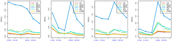
Figure 3. MSE of parameters in Table 2.

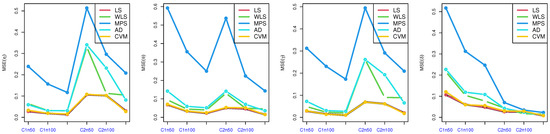
Figure 4. MSE of parameters in Table 3.

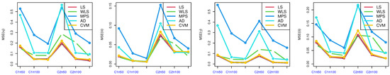
Figure 5. MSE of parameters in Table 4.

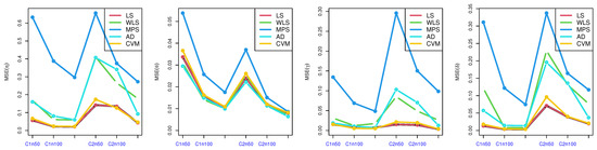
Figure 6. MSE of parameters in Table 5.

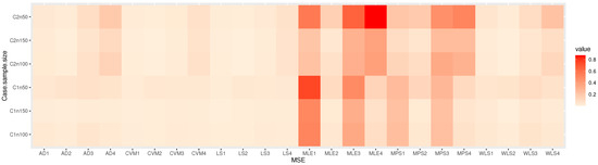
Figure 7. Heat-map of MSE for the parameters in Table 2.

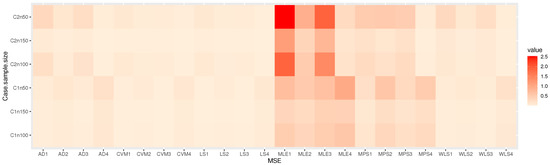
Figure 8. Heat-map of MSE for the parameters in Table 3.

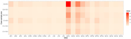
Figure 9. Heat-map of MSE for the parameters in Table 4.

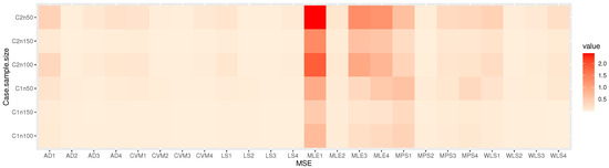
Figure 10. Heat-map of MSE for the parameters in Table 5.

The following conclusions can be drawn from Table 2, Table 3, Table 4 and Table 5:

• The results in the tables show that the TIIEHL-PLo distribution is stable since the range of bias and MSE for the four parameters of the TIIEHL-PLo distribution is fairly modest.
• As the sample size increases, we occasionally observe a decrease in the bias and MSE for all estimations.
• This indicates that, for high sample sizes, several estimating methodologies yield a correct bias and MSE findings.
• The LS and CVM estimation approach are the most accurate means of estimating the TIIEHL-PLo distribution parameter.
• Better metrics than the MLE approaches are provided by the LS, WLS, CVM, MPS, and AD estimation methods.

Through the previous tables and conclusions, we noticed that the two methods LS and CVM are very close, and we want to suggest the best method, so that the averages of the MSE values were calculated in Table 6. From Table 6, we noticed that the best way to estimate the parameters of the TIIEHL-PLo distribution is LS.

Table 6. Average MSE for the parameters of each estimation method.

		MLE	LS	WLS	MPS	CVM	AD
$\gamma$	n	$\eta =0.85,\theta =0.6,\delta =1.2$
0.7	50	0.3720	0.0346	0.0726	0.1935	0.0377	0.0617
	100	0.2508	0.0217	0.0417	0.1510	0.0226	0.0376
	150	0.2344	0.0173	0.0296	0.1394	0.0189	0.0195
1.8	50	0.5626	0.0353	0.1014	0.3440	0.0381	0.0867
	100	0.2533	0.0281	0.0567	0.2208	0.0307	0.0682
	150	0.2370	0.0265	0.0444	0.1657	0.0273	0.0529
$\eta$	n	$\theta =2,\gamma =1.8,\delta =1.2$
0.85	50	0.7303	0.0577	0.1056	0.4154	0.0637	0.1250
	100	0.4844	0.0317	0.0508	0.2639	0.0315	0.0600
	150	0.3869	0.0233	0.0419	0.1967	0.0265	0.0546
2	50	1.4071	0.0633	0.1910	0.4039	0.0651	0.1965
	100	1.0043	0.0588	0.0671	0.2116	0.0610	0.1296
	150	0.6292	0.0184	0.0635	0.1457	0.0168	0.0482
$\theta$	n	$\eta =3,\gamma =3,\delta =2$
1.2	50	0.6446	0.0855	0.0784	0.3327	0.0917	0.2624
	100	0.4521	0.0239	0.0437	0.1711	0.0247	0.0569
	150	0.2544	0.0216	0.0401	0.1177	0.0211	0.0510
3	50	2.1460	0.1137	0.1500	0.3291	0.1286	0.2996
	100	1.0592	0.0324	0.1216	0.1750	0.0351	0.0599
	150	0.6351	0.0240	0.0377	0.1190	0.0271	0.0515
$\delta$	n	$\eta =2.5,\theta =1.5,\gamma =3$
0.5	50	0.4633	0.0296	0.0877	0.2829	0.0342	0.0664
	100	0.3264	0.0125	0.0238	0.1510	0.0125	0.0301
	150	0.2179	0.0106	0.0236	0.1094	0.0105	0.0227
1.2	50	1.2784	0.0631	0.1875	0.3315	0.0793	0.1821
	100	0.9324	0.0500	0.1143	0.1762	0.0493	0.1396
	150	0.6555	0.0185	0.0718	0.1242	0.0199	0.0370

6. Modeling of Environmental and Medical Data

The TIIEHL-PLo distribution is used in this section to model several real data examples from many scientific domains. Different distributions, including the extended odd Weibull inverse Nadarajah–Haghighi (EOWINH) [26], Kumaraswamy Weibull (KW) [27], MOAPLo, Marshall–Olkin alpha power extended Weibull (MOAPEW) [28], ELo, IWLoPS, WLo, and GLo models, are offered for comparison with the TIIEHL-PLo model.

For all datasets, we compute the terms “Akaike information criterion (${\nabla }_1$), correct Akaike information criterion (${\nabla }_2$), Bayesian information criterion (${\nabla }_3$), and Hannan–Quinn information criterion (${\nabla }_4$)” were used to analyze the MLE with the standard error (SE) and various measures (${\nabla }_1$, ${\nabla }_2$, ${\nabla }_3$, and ${\nabla }_4$). The Kolmogorov–Smirnov goodness-of-fit test is used for real data, and the results show that the TIIEHL-PLo, EOWINH, GLo, MOAPLo, MOAPEW, ELo, KW, IWLoPS, and WL distributions fit each of the datasets according to the Kolmogorov–Smirnov distance (KS) and Kolmogorov–Smirnov p-value (PVKS).

6.1. Environmental Data

Data-I. Acid rain is a frequent environmental occurrence caused by the high concentrations of nitric and sulfuric acids in the atmosphere that are carried to Earth and have an impact on a variety of ecological factors, including the diversity of species, the abundance of worms, the size of crabs, the quality of water, the physiological state of individual animals, etc. The oxidation of sulfur and nitrogen in coal and other fossil fuels leads to the creation of acidic pollutants in the atmosphere. Acid rain has seriously destroyed forests in several industrialized nations. Utilizing coal and low-sulfur fuel will help prevent acid rain. In this section, environmental calamities are discussed. On a pH scale, which ranges from one (very acidic) to seven, acidity is measured (neutral). A pH of less than 5.7 is thought to be the threshold for acid rain. The first set of data examines the acidity of Minnesota’s rains during a forty-day period. The values of this dataset, which was published by [32], are as follows: “3.71, 4.23, 4.16, 2.98, 3.23, 4.67, 3.99, 5.04, 4.55, 3.24, 2.80, 3.44, 3.27, 2.66, 2.95, 4.70, 5.12, 3.77, 3.12, 2.38, 4.57, 3.88, 2.97, 3.70, 2.53, 2.67, 4.12, 4.80, 3.55, 3.86, 2.51, 3.33, 3.85, 2.35, 3.12, 4.39, 5.09, 3.38, 2.73, and 3.07”. Figure 11 describes Environmental data-I using box plot, strip plot, and Violine plot of data to check that the data do not have outlier problems and whether the data have symmetric ships. Environmental data-I was reported to be asymmetrical, and uncertain outlier observations were confirmed.

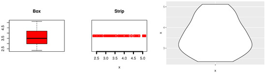
Figure 11. Box, strip and Violin plots of Environmental data-I.

Table 7 obtained the MLE with SE values of parameters of each comparative model as TIIEHL-PLo, EOWINH, KW, MOAPLo, MOAPEW, ELo, IWLoPS, WLo, and GLo distribution. Furthermore, different measures of the goodness of fit were obtained to compare these models. Figure 12 discusses the estimation of the TIIEHL-PLo distribution for Environmental data-I, where I is the empirical cdf of Environmental data-I, II is the estimated pdf with the histogram of Environmental data-I, III is the QQ plot of data and generates a sample of the TIIEHL-PLo distribution for Environmental data-I, and IV is the plotted PP plot of the TIIEHL-PLo distribution for Environmental data-I. From the results in Table 7 and Figure 12, the TIIEHL-PLo distribution fit of Environmental data-I is confirmed. Figure 13 discusses the profile likelihood of TIIEHL-PLo of Environmental data-I and confirmed the estimators have maximum points. Table 8 discusses the estimation of parameters based on a different estimation method. From the results in Table 8, the LS and WLS method are the best estimation method, whereas the KS distance is small and PVKSs are larger than another methods.

Table 7. MLE estimators with goodness-of-fit measures: Environmental data-I.

Models		Estimates	SE	${\mathit{\nabla }}_1$	${\mathit{\nabla }}_3$	${\mathit{\nabla }}_2$	${\mathit{\nabla }}_4$	CVM	AD	KS	PVKS
TIIEHL-PLo	$\eta$	0.0547	0.0025	101.4707	108.2262	102.6136	103.9133	0.0423	0.3147	0.0764	0.9738
	$\theta$	11.9313	6.5648
	$\gamma$	10.2097	5.2268
	$\delta$	120.4763	26.4693
EOWINH	$\alpha$	7.7423	2.4349	102.4427	103.5855	109.1982	104.8853	0.0427	0.3298	0.0809	0.9560
	$\beta$	0.4600	0.5247
	$\lambda$	0.9827	0.9747
	$\theta$	5.7681	4.7740
KW	$\alpha$	0.1322	0.0142	99.2020	100.3448	105.9575	101.6446	0.0255	0.2087	0.0656	0.9954
	$\beta$	3.3827	0.0097
	$\lambda$	13.7096	0.5152
	$\theta$	0.1023	0.0214
MOAPLo	$\alpha$	294.3313	21.2626	105.5206	106.6635	112.2761	107.9632	0.0698	0.4915	0.0828	0.9469
	$\beta$	27.7774	23.9966
	$\lambda$	1180.6838	39.5466
	$\theta$	9.5382	9.3425
MOAPEW	$\alpha$	54.5650	140.1735	107.1567	108.9214	115.6011	110.2099	0.0791	0.5424	0.0808	0.9567
	$\beta$	2.9115	2.1861
	$\lambda$	0.8447	2.3056
	$\theta$	24.1657	112.4007
	$\delta$	17.6442	118.2467
ELo	$\alpha$	137.985746	112.6857	101.3571	108.80238	105.42374	104.18904	0.043415	0.336339	0.085706	0.930577
	$\beta$	75.35675	219.6866
	$\lambda$	47.6452043	149.0872
IWLoPS	$\alpha$	0.0540	0.0301	101.9895	103.1323	108.7450	104.4321	0.0479	0.3487	0.0773	0.9706
	$\beta$	345.6694	190.0276
	$\lambda$	99.8438	52.5460
	$\theta$	1.2466	0.9456
WLo	$\alpha$	1.6850	3.6630	103.5711	104.7139	110.3266	106.0137	0.0771	0.5231	0.0947	0.8655
	$\beta$	10.3668	9.1686
	$\lambda$	0.2485	0.2101
	$\theta$	0.2855	0.9960
GLo	$\alpha$	103.5638	357.9515	102.2910	103.4338	109.0465	104.7335	0.0431	0.3341	0.0852	0.9334
	$\beta$	73.8117	277.9995
	$\lambda$	0.9181	1.7041
	$\theta$	122.1513	132.8174

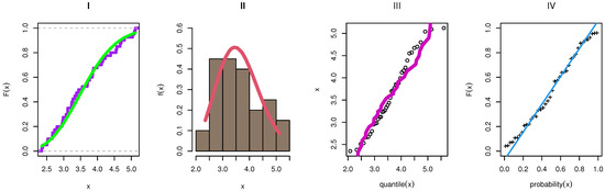
Figure 12. The estimation of the TIIEHL-PLo distribution: Environmental data-I.

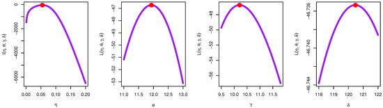
Figure 13. Profile likelihood of TIIEHL-PLo: Environmental data-I.

Table 8. Estimation methods and KS test: Environmental data-I.

	MLE	LS	WLS	MPS	CVM	AD
$\eta$	0.0547	0.0357	0.0665	0.0500	0.0414	0.0436
$\theta$	11.9313	17.1084	9.0774	11.7787	12.8477	13.4472
$\gamma$	10.2097	8.9407	8.9112	9.1147	8.2366	8.9022
$\delta$	120.4763	88.0345	92.3735	120.8870	123.9244	109.8484
KS	0.0764	0.0563	0.0558	0.0611	0.0603	0.0582
PVKS	0.9738	0.9996	0.9996	0.9983	0.9986	0.9993

6.2. Medical Data

Data-I: Barco et al. [33] used this dataset as “1.1, 1.4, 1.3, 1.7, 1.9, 1.8, 1.6, 2.2, 1.7, 2.7, 4.1, 1.8, 1.5, 1.2, 1.4, 3.0, 1.7, 2.3, 1.6, 2.0”, which the information displays how quickly 20 people felt better after taking an analgesic. Figure 14 discusses the description of Medical data-I using the box plot, strip plot, and Violine plot of the data to check that Medical data-I does not have outlier problems and whether the data have symmetric ships. Medical data-I was reported to be asymmetrical, and certain outlier observations were confirmed.

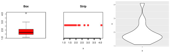
Figure 14. Box, strip and Violin plot of Medical data-I.

Table 9 obtained an MLE with the SE values of the parameters of each comparative model as TIIEHL-PLo, EOWINH, KW, MOAPLo, MOAPEW, ELo, IWLoPS, WLo, and GLo distribution. Furthermore, different goodness-of-fit measures were obtained to compare these models. Figure 15 discusses the estimation of the TIIEHL-PLo distribution for Medical data-I, where I is the empirical cdf of Medical data-I, II is the estimated pdf with the histogram of Medical data-I, III is the QQ plot of the data and generates a sample of the TIIEHL-PLo distribution for Medical data-I, and IV is the PP plot of the TIIEHL-PLo distribution for Medical data-I. From the results in Table 9 and Figure 15, the TIIEHL-PLo distribution fit of Medical data-I is confirmed. Figure 16 discusses the profile likelihood of the TIIEHL-PLo of Medical data-I and confirms that the estimators have maximum points. Table 10 discusses the estimation of parameters based on different estimation methods. The results in Table 10 evidence that the CVM method is the best estimation method when the KS distance is small and the PVKS is larger than another methods.

Table 9. MLE estimators with goodness-of-fit measures: Medical data-I.

Models		Estimates	SE	${\mathit{\nabla }}_1$	${\mathit{\nabla }}_3$	${\mathit{\nabla }}_2$	${\mathit{\nabla }}_4$	CVM	AD	KS	PVKS
TIIEHL-PLo	$\eta$	9.5189	2.5157	38.7871	42.7700	41.4538	39.5646	0.0266	0.1515	0.0952	0.9935
	$\theta$	0.6046	0.5165
	$\gamma$	4544.7074	25.5165
	$\delta$	1.0583	0.8994
EOWINH	$\alpha$	146.9404	1.3401	43.2241	45.8908	47.2070	44.0016	0.0971	0.5746	0.1686	0.6202
	$\beta$	5.0325	0.1032
	$\lambda$	10.7858	1.0159
	$\theta$	0.8082	1.3055
KW	$\alpha$	2.1289	0.7607	41.1433	43.8099	45.1262	41.9208	0.0627	0.3691	0.1488	0.7679
	$\beta$	0.8551	0.3273
	$\lambda$	28.9148	24.2893
	$\theta$	1.2803	1.1606
MOAPLo	$\alpha$	546,390.9153	225.1516	44.8576	47.5243	48.8405	45.6351	0.1168	0.6871	0.1290	0.8931
	$\beta$	1,287,898.0703	2356.5153
	$\lambda$	8.6949	3.1731
	$\theta$	475,204.4105	130.0856
MOAPEW	$\alpha$	38.8928	41.7939	48.5882	52.8739	53.5669	49.5601	0.1341	0.7925	0.1517	0.7467
	$\beta$	2.5248	0.6696
	$\lambda$	0.1090	0.1214
	$\theta$	32.1868	12.1517
	$\delta$	25.2059	34.5792
ELo	$\alpha$	77.2175	116.8405	39.1512	43.0124	41.9955	39.9549	0.0391	0.2260	0.1211	0.9308
	$\beta$	12.0930	17.6372
	$\lambda$	3.6927	7.7470
IWLoPS	$\alpha$	1.3286	5.8583	38.8502	42.8152	42.8331	39.6277	0.0253	0.1457	0.0945	0.9941
	$\beta$	3.0159	8.0370
	$\lambda$	11.6474	59.2088
	$\theta$	1.0065	1.5240
WLo	$\alpha$	8.3496	34.5554	47.3153	49.9820	51.2982	48.0928	0.1575	0.9298	0.1790	0.5430
	$\beta$	5.6433	4.1698
	$\lambda$	0.2286	0.2052
	$\theta$	0.2380	0.6492
GLo	$\alpha$	1.6185	4.0536	38.7894	42.8456	42.7723	39.5669	0.0285	0.1610	0.0961	0.9926
	$\beta$	1.1993	0.5152
	$\lambda$	0.3103	0.3337
	$\theta$	30.0251	8.2652

Figure 15. The estimation of the TIIEHL-PLo distribution: Medical data-I.

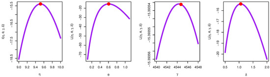
Figure 16. Profile likelihood of TIIEHL-PLo: Medical data-I.

Table 10. Estimation methods and KS test: Medical data-I.

	MLE	LS	WLS	MPS	CVM	AD
$\eta$	9.5189	9.9205	9.7301	11.1211	9.4695	9.5634
$\theta$	0.6046	0.5250	0.5259	0.7125	0.5733	0.5682
$\gamma$	4544.7074	5552.7217	4547.8144	4602.8831	4548.3921	4544.2005
$\delta$	1.0583	1.1914	1.1224	0.1279	1.2596	1.1490
KS	0.0952	0.0945	0.1011	0.4691	0.0890	0.0941
PVKS	0.9935	0.9943	0.9868	0.0003	0.9974	0.9944

Data-II: The most recent data, cited by [34], which shows the number of daily confirmed death cases linked to COVID-19. The dataset is given as follows: “1.00, 1.00, 2.00, 4.00, 5.00, 1.00, 1.00, 3.00, 6.00, 6.00, 4.00, 1.00, 5.00, 6.00, 6.00, 8.00, 5.00, 7.00, 7.00, 9.00, 9.00, 15.00, 17.00, 11.00, 13.00, 5.00, 14.00, 5.00, 13.00, 9.00, 19.00, 15.00, 11.00, 14.00, 12.00, 11.00, 7.00, 13.00, 10.00, 20.00, 22.00, 21.00, 12.00, 14.00, 9.00, 14.00, 7.00, 16.00, 17.00, 13.00, 21.00, 11.00, 11.00, 8.00, 11.00, 12.00, 15.00, 21.00, 20.00, 18.00, 15.00, 14.00, 21.00, 16.00, 11.00, 28.00, 29.00, 19.00, 14.00, 19.00, 29.00, 34.00, 34.00, 46.00, 46.00, 47.00, 36.00, 38.00, 40.00, 32.00, 39.00, 34.00, 35.00, 36.00, 35.00, 45, 62” The data consists of 89 observed values. Figure 17 describes Medical data-II using box plot, strip plot, and Violine plot of the data to verify whether Medical data-II has any outlier problems and whether the data have symmetric ships. Medical data-II was reported to be asymmetrical, and certain outlier observations were confirmed.

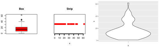
Figure 17. Box, strip and Violin plot of Medical data-II.

Table 11 shows the MLE with the SE values of the parameters of each comparative model as TIIEHL-PLo, EOWINH, KW, MOAPLo, MOAPEW, ELo, IWLoPS, WLo, and GLo distribution. Furthermore, different goodness-of-fit measures are obtained to compare these models. Figure 18 discusses the estimation of the TIIEHL-PLo distribution for Medical data-II, where I is the empirical cdf of Medical data-II, II is the estimated pdf with the histogram of Medical data-II, III is the QQ plot of data and generates a sample of the TIIEHL-PLo distribution for Medical data-II, and IV is the PP plot of the TIIEHL-PLo distribution for Medical data-II. The results in Table 11 and Figure 18 confirm the TIIEHL-PLo distribution fit of Medical data-II. Table 12 discusses the estimation of parameters based on different estimation methods. The results in Table 12 evidence that the LS method is the best estimation method when the KS distance is small and the PVKS is larger than other methods.

Table 11. MLE estimators with goodness-of-fit measures: COVID-19 data.

Models		Estimates	SE	${\mathit{\nabla }}_1$	${\mathit{\nabla }}_3$	${\mathit{\nabla }}_2$	${\mathit{\nabla }}_4$	CVM	AD	KS	PVKS
TIIEHL-PLo	$\eta$	1.8085	1.2965	664.2789	674.1425	664.7667	668.2506	0.0817	0.6012	0.0710	0.7725
	$\theta$	0.1161	0.0952
	$\gamma$	41.3607	21.2156
	$\delta$	6812.653	178.7555
EOWINH	$\alpha$	143.3842	51.2157	669.3280	679.8158	679.1916	673.2997	0.1287	1.0204	0.1241	0.1370
	$\beta$	133.7293	303.9769
	$\lambda$	33.8102	20.1257
	$\theta$	0.4976	0.3460
KW	$\alpha$	0.0808	0.2125	664.8686	674.3564	673.7322	669.8404	0.0911	0.6100	0.0739	0.7284
	$\beta$	1.2726	0.2508
	$\lambda$	1.1680	0.5009
	$\theta$	0.3210	0.9742
MOAPLo	$\alpha$	0.0269	0.0419	664.3716	674.5594	673.9352	668.4334	0.0823	0.6184	0.0731	0.7413
	$\beta$	90.5058	30.9432
	$\lambda$	15.1273	11.1261
	$\theta$	1104.807	861.105
MOAPEW	$\alpha$	5.4995	6.7764	673.4946	674.9235	685.8242	678.4593	0.2217	1.2727	0.0914	0.4609
	$\beta$	0.2972	0.1458
	$\lambda$	5.1496	11.4986
	$\theta$	1.5716	4.0306
	$\delta$	0.2669	0.5105
ELo	$\alpha$	1.812536	0.316325	665.7241	674.2132	671.1218	669.7029	0.086053	0.618995	0.084499	0.563524
	$\beta$	11.24635	8.116818
	$\lambda$	123.1732	102.2685
IWLoPS	$\alpha$	2.8782	0.5064	665.1901	675.6779	675.0538	669.1619	0.0808	0.6352	0.0851	0.5537
	$\beta$	0.1144	0.0168
	$\lambda$	75.6522	28.3858
	$\theta$	318.7325	95.4457
WLo	$\alpha$	0.1965	4.4704	664.9076	674.3954	673.7712	668.8794	0.0929	0.6170	0.0750	0.7125
	$\beta$	1.4744	0.8668
	$\lambda$	0.8391	0.5010
	$\theta$	4.3238	70.5703
GLo	$\alpha$	44.9638	69.7191	664.3935	674.4225	673.7984	668.9065	0.0848	0.6160	0.0749	0.7138
	$\beta$	127.8803	85.2441
	$\lambda$	3.1249	1.1160
	$\theta$	3.0512	0.7620

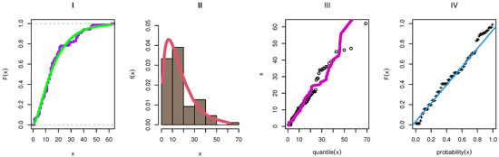
Figure 18. The estimated of TIIEHL-PLo distribution: Medical data-II.

Table 12. Estimation methods and KS test: Medical data-II.

	MLE	LS	WLS	CVM	AD
$\eta$	1.8085	2.5624	1.8118	1.9405	1.8150
$\theta$	0.1161	0.1006	0.1154	0.1137	0.1143
$\gamma$	41.3607	70.4544	41.4426	46.6119	41.4314
$\delta$	6812.6527	2457.0208	6813.0472	6834.7056	6812.6556
KS	0.0710	0.0696	0.0685	0.0705	0.0697
PVKS	0.7725	0.7933	0.8085	0.7807	0.7913

7. Conclusions and Summary

In this article, we introduced and studied the type II exponentiated half-logistic-PLo (TIIEHL-PLo) model as a new extension of the PLo model. The new TIIEHL-PLo model is more flexible and applicable than the PLo model and some well-known statistical models, especially in environmental and medical sciences. The pdf for the TIIEHL-PLo model can be uni-modal, decreasing, right skewed, and heavy-tailed. However, the hrf can be decreasing, upside-down, and J-shaped. Some fundamental statistical characteristics of the TIIEHL-PLo model such as the QF, the nth raw moments, mean, variance, skewness, kurtosis, moment-generating function, many graphical and numerical results of moments, and order statistics were calculated. Six different estimation approaches—namely the ML, LS, WLS, MPS, CVM, and AD estimation approaches—were utilized to estimate the parameters of the TIIEHL-PLo model. The simulation experiment examined the accuracy of the model parameters by employing six various estimation techniques. In this study, we analyzed three real datasets from the environmental and medical sciences to show the relevance and adaptability of the TIIEHL-PLo model. The new TIIEHL-PLo model achieves the best fit and performance when we compared it with several well-known statistical models.

References

- Lomax, K.S. Business failures: Another example of the analysis of failure data. J. Am. Stat. Assoc. 1954, 49, 847–852. [Google Scholar] [CrossRef]
- Hassan, A.; Al-Ghamdi, A. Optimum step stress accelerated life testing for Lomax distribution. J. Appl. Sci. Res. 2009, 5, 2153–2164. [Google Scholar]
- Atkinson, A.; Harrison, A. Distribution of Personal Wealth in Britain; Cambridge University Press: Cambridge, UK, 1978. [Google Scholar]
- Harris, C. The Pareto distribution as a queue service discipline. Oper. Res. 1968, 16, 307–313. [Google Scholar] [CrossRef]
- Chen, J.; Addie, R.G.; Zukerman, M.; Neame, T.D. Performance evaluation of a queue fed by a Poisson Lomax Burst Process. IEEE Commun. Lett. 2015, 19, 367–370. [Google Scholar] [CrossRef]
- Ghitany, M.E.; Al-Awadhi, F.A.; Alkhalfan, L.A. Marshall Olkin extended Lomax distribution and its application to censored data. Commun. Stat. Theory Methods 2007, 36, 1855–1866. [Google Scholar] [CrossRef]
- Abdul-Moniem, I.B.; Abdel-Hameed, H.F. On exponentiated Lomax distribution. Int. J. Math. Arch. 2012, 3, 2144–2150. [Google Scholar]
- Ashour, S.K.; Eltehiwy, M.A. Transmuted Lomax distribution. Am. J. Appl. Math. Stat. 2013, 1, 121–127. [Google Scholar] [CrossRef]
- Lemonte, A.J.; Cordeiro, G.M. An extended Lomax distribution. Statistics 2013, 47, 800–816. [Google Scholar] [CrossRef]
- Al-Zahrani, B.; Sagor, H. The Poisson-Lomax distribution. Rev. Colomb. Estad. 2014, 37, 225–245. [Google Scholar] [CrossRef]
- El-Bassiouny, A.H.; Abdo, N.F.; Shahen, H.S. Exponential Lomax distribution. Int. J. Comput. Appl. 2015, 121, 24–29. [Google Scholar]
- Cordeiro, G.M.; Ortega, E.M.; Popovíc, B.V. The gamma Lomax distribution. J. Stat. Comput. Simul. 2015, 85, 305–319. [Google Scholar] [CrossRef]
- Tahir, M.H.; Cordeiro, G.M.; Mansoor, M.; Zubair, M. The Weibull-Lomax distribution: Properties and applications. Hacet. J. Math. Stat. 2015, 44, 461–480. [Google Scholar] [CrossRef]
- Kilany, N.M. Weighted Lomax distribution. SpringerPlus 2016, 5, 1862. [Google Scholar] [CrossRef]
- Oguntunde, P.E.; Khaleel, M.A.; Ahmed, M.T.; Adejumo, A.O.; Odetunmibi, O.A. A New Generalization of the Lomax Distribution with Increasing, Decreasing and Constant Failure Rate. Model. Simul. Eng. 2017, 2017, 6043169. [Google Scholar] [CrossRef]
- Hassan, A.S.; Elgarhy, M.; Mohamed, R.E. Statistical Properties and Estimation of Type II Half Logistic Lomax Distribution. Thail. Stat. 2020, 18, 290–305. [Google Scholar]
- Tahir, M.H.; Hussain, M.A.; Cordeiro, G.M.; Hamedani, G.G.; Mansoor, M.; Zubair, M. The Gumbel-Lomax distribution: Properties and applications. J. Stat. Theory Appl. 2016, 15, 61–79. [Google Scholar] [CrossRef]
- Rady, E.A.; Hassanein, W.A.; Elhaddad, T.A. The power Lomax distribution with an application to bladder cancer data. SpringerPlus 2016, 5, 1838. [Google Scholar] [CrossRef]
- Moltok, T.T.; Dikko, H.G.; Asiribo, O.E. A transmuted Power Lomax distribution. Afr. J. Nat. Sci. 2017, 20, 67–78. [Google Scholar]
- Al-Marzouki, S. A new generalization of power Lomax distribution. Int. J. Math. Math. Sci. 2018, 7, 59–68. [Google Scholar]
- Assar, S.M. On odds generalized exponential-power Lomax distribution. J. Math. Stat. 2018, 14, 167–174. [Google Scholar] [CrossRef]
- Hassan, A.S.; Abd-Allah, M. On the inverse power Lomax distribution. Ann. Data Sci. 2019, 6, 259–278. [Google Scholar] [CrossRef]
- Al-Marzouki, S.; Jamal, F.; Chesneau, C.; Elgarhy, M. Type II Topp Leone Power Lomax Distribution with Applications. Mathematics 2020, 8, 4. [Google Scholar] [CrossRef]
- Algarni, A. Sine Power Lomax Model with Application to Bladder Cancer Data. Nanosci. Nanotechnol. Lett. 2020, 12, 677–684. [Google Scholar]
- Al-Mofleh, H.; Elgarhy, M.; Afify, A.Z.; Zannon, M.S. Type II exponentiated half logistic generated family of distributions with applications. Electron. J. Appl. Stat. Anal. 2020, 13, 36–561. [Google Scholar]
- Almetwally, E.M. Extended odd weibull inverse Nadarajah-Haghighi distribution with application on COVID-19 in Saudi Arabia. Math. Sci. Lett. Int. J. 2021, 10, 85–99. [Google Scholar]
- Cordeiro, G.M.; Ortega, E.M.; Nadarajah, S. The Kumaraswamy Weibull distribution with application to failure data. J. Frankl. Inst. 2010, 347, 1399–1429. [Google Scholar] [CrossRef]
- Almetwally, E.M. Marshall olkin alpha power extended Weibull distribution: Different methods of estimation based on type i and type II censoring. Gazi Univ. J. Sci. 2022, 35, 293–312. [Google Scholar]
- MacGillivray, H.L. Skewness and asymmetry: Measures and orderings. Ann. Stat. 1986, 14, 994–1011. [Google Scholar] [CrossRef]
- Macdonald, P.D.M. Comments and queries comment on “an estimation procedure for mixtures of distributions” by choi and bulgren. J. R. Stat. Soc. Ser. B (Methodol.) 1971, 33, 326–329. [Google Scholar] [CrossRef]
- Swain, J.J.; Venkatraman, S.; Wilson, J.R. Least-squares estimation of distribution functions in Johnson’s translation system. J. Stat. Comput. Simul. 1988, 29, 271–297. [Google Scholar] [CrossRef]
- Ross, M.S. Introductory Statistics, 3rd ed.; Elsevier: Oxford, UK, 2010; p. 365. [Google Scholar]
- Barco, K.V.P.; Mazucheli, J.; Janeiro, V. The inverse power Lindley distribution. Commun. Stat.-Simul. Comput. 2017, 46, 6308–6323. [Google Scholar] [CrossRef]
- Alyami, S.A.; Elbatal, I.; Alotaibi, N.; Almetwally, E.M.; Okasha, H.M.; Elgarhy, M. Topp-Leone Modified Weibull Model: Theory and Applications to Medical and Engineering Data. Appl. Sci. 2022, 12, 10431. [Google Scholar] [CrossRef]
Disclaimer/Publisher’s Note: The statements, opinions and data contained in all publications are solely those of the individual author(s) and contributor(s) and not of MDPI and/or the editor(s). MDPI and/or the editor(s) disclaim responsibility for any injury to people or property resulting from any ideas, methods, instructions or products referred to in the content. |
© 2023 by the authors. Licensee MDPI, Basel, Switzerland. This article is an open access article distributed under the terms and conditions of the Creative Commons Attribution (CC BY) license (https://creativecommons.org/licenses/by/4.0/).