Abstract
This paper deals with the statistical inference of the unknown parameter and some life parameters of inverse Lindley distribution under the assumption that the data are adaptive Type-II progressively censored. The maximum likelihood method is considered to acquire the point and interval estimates of the distribution parameter, reliability, and hazard rate functions. The approximate confidence intervals are also addressed. The delta method is taken into consideration to approximate the variances of the estimators of the reliability and hazard rate functions to get the required intervals. Based on the assumption of gamma prior, we further consider Bayesian estimation of the different parameters. The Bayes estimates are obtained by considering squared error and general entropy loss functions. The Bayes estimates and highest posterior density credible intervals are obtained by employing the Markov chain Monte Carlo procedure. An exhaustive numerical study is conducted to compare the offered estimates with regard to their root means squared error, relative absolute biases, confidence lengths, and coverage probabilities. To explain the suggested methods, two applications are investigated. The numerical findings show that the Bayes estimates perform better than those obtained based on the maximum likelihood method. The Bayesian estimations using the asymmetric loss function give more efficient estimates than the symmetric loss. Finally, the inverse Lindley distribution is recommended to be used as a suitable model to fit airborne communication transceiver and wooden toys data sets when compared with some competitive models including inverse Weibull, inverse gamma and alpha power inverted exponential.
Keywords:
inverse Lindley model; reliability analysis; Bayes inference; MCMC techniques; maximum likelihood; adaptive progressive hybrid censoring MSC:
62F10; 62F15; 62N01; 62N02; 62N05
1. Introduction
As a combination of exponential and gamma distributions, Lindley [1] established the so-called Lindley distribution (LD). Because LD is only useful for modelling data with a monotonically increasing failure rate, its relevance may be limited to data with non-monotone shapes, such as upside-down bathtub shapes. Sharma et al. [2] offered the inverse Lindley (IL) distribution, which has an upside-down bathtub-shaped hazard rate function (HRF), as an inverted counterpart of the LD distribution. Assume that Y is a random variable with the IL distribution, represented by the symbol , where is a scale parameter. According to Sharma et al. [2], for , the associated probability density function (PDF), reliability function (RF), and HRF, are given, respectively, by
and
Basu et al. [3] considered the estimations of IL distribution using Type-I censored data. Basu et al. [4] studied some estimation problems of IL distribution using progressive hybrid Type-I censoring scheme with binomial removals. Basu et al. [5] investigated the maximum likelihood, product of spacing and Bayesian estimations for IL based on hybrid censored data. Hassan et al. [6] studied the inference about reliability parameter for IL distribution based on ranked set sampling.
The life-testing experiments frequently end before all of the objects fail. it occurs because of time restrictions or a lack of funding. The observations that arise from these scenarios are referred to as the censored sample. Numerous censoring techniques have been presented in the literature. Of these, the progressive censoring plan is highly helpful since it enables the removal of a predetermined number of surviving items at various periods. Adaptive Type-II progressive hybrid censoring (T2-APHC), proposed by Ng et al. [7], has received a lot of attention from several authors because it allows for the production of highly efficient statistical analysis. In this plan, the total test items n units are placed on a test at time zero, the number of failures is predetermined, and the testing time is permitted to run over the prefixed time T. Also, the progressive censoring is prefixed, but some of its values may be adjusted consequently during the test. When the first failure occurs, units are randomly removed from the test. Similarly, when the second failure occurs, units are randomly removed and so on. If the failure occurs before time T , the test stops at the failure and we have . On the other hand, if the failure occurs before time T (i.e., ), where and , we change the removal pattern bt setting for , then we have . This mechanism ensures that the test will stop when the experimenter achieves the desired number of failures m, and that the overall test duration will be close to the optimal time T. However, suppose is a T2-APHC sample obtained from a continuous population, then according to Ng et al. [7] the likelihood function of the observed data can be defined as
where C is a constant and is used instead of for simplicity. In the past decade, using T2-APHC plan, several authors have derived different point and/or interval estimators of various parameters of life, for example; see Al Sobhi et al. [8], Hemmati and Khorram [9], Nassar et al. [10], Panahi and Moradi [11], Elshahhat and Nassar [12], Panahi and Asadi [13], Du and Gui [14], Alotaibi et al. [15], Alotaibi et al. [16], Ateya et al. [17], Elshahhat and Nassar [18], and references cited therein.
We are motivated to perform this work because (1) The IL distribution exhibits two very admirable characteristics. In addition to possessing a hazard function with an upside-down bathtub shape, which is a common occurrence in many domains, it is a single parameter distribution, which greatly smoothes out the mathematical difficulties. (2) The effectiveness of the T2-APHC plan in reducing the overall test duration while preserving the desired characteristics of progressive censoring in practical reliability studies. From the aforementioned development, it is evident that the problem of estimating the unknown parameter, RF, and HRF of the IL distribution based on the T2-APHC sample has not been explored. Therefore, we can say that our main objective in this study is to investigate some estimation issues for the IL distribution when the data are T2-APHC. We first obtain the maximum likelihood estimates (MLEs) of the various parameters as classical estimates as well as the approximate confidence intervals (ACIs). We further use the Bayesian estimation method to obtain the Bayes estimates and the highest posterior density (HPD) credible intervals based on gamma prior. The Bayes estimates are obtained through the Markov chain Monte Carlo (MCMC) technique. Two loss functions are taken into consideration for this purpose. The first is the squared error (SE) loss function as a symmetric one. The second is the general entropy (GE) loss function which is an asymmetric loss function. The effectiveness of the various strategies is examined through extensive simulations, and two actual data sets have been examined for illustration.
The remainder of the paper is structured as follows. In Section 3, the maximum likelihood method is applied to acquire the MLEs of the various parameters , RF, and HRF and the associated ACIs. Using gamma prior, two loss functions and the MCMC procedure, we provide the Bayesian estimation, including point and HPD credible intervals, of the unknown parameters in Section 3. A simulation study is performed and its outcomes are presented in Section 4. Two real data sets are analyzed and displayed in Section 5. Finally, Section 6 concludes the paper.
2. Classical Inference
In this section, the maximum likelihood method is taken into consideration to acquire the model parameter estimates as well as its RF and HRF. Additionally, the ACIs of the various parameters are created based on the asymptotic nature of the MLEs. It is crucial to note that the RF and HRF estimators’ variances are calculated using the delta approach since these functions’ variances cannot be obtained explicitly. Suppose that be a T2-APHC sample of size m with from the IL distribution. The likelihood function in this instance can be determined from (1), (2) and (4), after omitting the constant term, as follows
where for the sake of simplicity. By using the natural logarithm of (5), we can determine the log-likelihood function for the case under consideration as follows
In this context, the MLE of the model parameter , symbolized by , can be owned by maximizing (6) with respect to , or otherwise, by solving the resulting equation
There is no closed-form for the MLE , as can be seen from (7). Therefore, a numerical method may be used to solve (7) in order to obtain the MLE of .
One of the main issues in maximum likelihood estimation is how to prove the existence and uniqueness of the acquired MLE . Due to the complex form of (7), by simulating a T2-APHC sample with , and , both the existence and uniqueness of are graphically proved in Figure 1, which presents the log-likelihood function in (6) and the normal equation in (7). As a result, the MLE of is 2.099918. It is clear, from Figure 1, that the offered maximum likelihood value of exists and is unique.
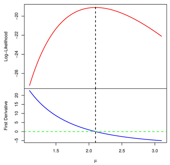
Figure 1.
The log-likelihood function of from simulated T2-APHC data.
Utilizing the MLE’s invariance property to estimate RF and HRF is all that is necessary once has been determined. We can get the MLEs of RF and HRF at mission time t from (2) and (3), respectively, by substituting the parameter with the corresponding MLE , as shown below
and
The common asymptotic normality of the MLE can be applied to create the ACI for the parameter with estimated variance, denoted by , obtained from the inverse of the observed Fisher information matrix, which obtained based on the inverse of the matrix of second derivative of (6) and locally at the MLE of . From the log-likelihood function in (6), we obtain the second derivative of with respect to as follows
where , and . As a result, the ACI of the parameter can be constructed with level of confidence as follows
where is the upper percentile point of the standard normal distribution and is obtained as follows
We also need to determine the variances for the MLEs of RF and HRF, on the other hand, in order to build the ACIs for these functions. We apply the delta approach to obtain approximations of the variances of and . The delta method is a general strategy for calculating confidence intervals for any functions of MLEs. It takes a function that is too complex to calculate the variance analytically, approximates it linearly, and then calculates the variance of the linear function that is simpler and may be utilized for large sample inference, see for more detail Greene [19]. To get the required approximate estimated variances, we first need to obtain the following
and
Let and , then we can approximate the required variances of and , respectively, as
Thus, with level of confidence, the ACIs of RF and HRF can be computed, respectively, as follow
3. Bayesian Inference
This section deals with developing the Bayes estimators along with their HPD credible intervals of , and . Following the main features of the gamma density, reported by Sharma et al. [2], the IL parameter is assumed to have a gamma () density prior, where a and b are assumed to be known. However, combining the likelihood and gamma density functions of into the continuous Bayes’ theorem, the joint posterior PDF of can be written as
where .
Loss functions in the Bayesian paradigm perform a critical role because they can be used to identify overestimation and underestimation of a study of interest. We thus take into account one symmetric loss, namely the SE loss function, and one asymmetric loss, namely the GE loss function. Regarding the SE loss, it is well known that the Bayes estimator (say ) of is the posterior mean as
On the other hand, the GE loss offers a significance importance in both overestimation and underestimation. The GE loss, introduced by Calabria and Pulcini [20], is
where is the parameter loss that determines the degree of asymmetry. Under GE loss, the Bayes estimator (say ) of is given by
provided that exists and is finite.
It is clear, from (11), that the posterior PDF of cannot be expressed explicitly or reduced to any familiar distribution. Therefore, to compute the Bayes estimates of , and or to create their HPD intervals, we suggest generating MCMC samples from (11) using the Metropolis-Hastings (M-H) sampler, for detail see Gelman et al. [21] and Lynch [22]. It is of interest to mention here that some approximations like Lindley’s approximation and Tierney and Kadane’s approximation can be used to obtain the Bayes estimates in such situations. The main disadvantages of these method are (1) they give only point estimates for the unknown parameters and they cannot tell us anything regarding the HPD credible intervals, (2) to acquire the needed estimates we should deal with very complicated expressions, especially the third order derivatives. To overcome these difficulties, the M-H technique can be performed using the following steps:
- Step-1:
- Set the starting point .
- Step-2:
- Set .
- Step-3:
- Create from .
- Step-4:
- Finding .
- Step-5:
- Generate a sample u from the uniform distribution.
- Step-6:
- If , set ; otherwise, set .
- Step-7:
- Set .
- Step-8:
- Redo Steps 3–7 times to get for .
- Step-9:
- Ignore the first simulated samples (say ), to discard the impact of an initial guess, where .
- Step-10:
- Compute the reliability and hazard rate parameters (for ) via replacing by its MCMC variates .
- Step-11:
- Compute the Bayes estimates of (for example) under SE and GE loss functions asandrespectively.
- Step-12:
- Compute the HPD interval of by ordering the simulated samples of for as . Then, according to the method introduced by Chen and Shao [23], the two-sided HPD interval of can be given aswhere is selected such that
- Step-13:
- Redo Steps 11–12 for the time parameters and at distinct time .
4. Monte Carlo Simulation
In this section, via different Monte Carlo simulations, the performance of the proposed point and interval estimators of the IL parameter , reliability function , and hazard function is compared when an adaptive Type-II progressive hybrid strategy is implemented. Without sacrificing generality, we simulate 1000 T2-APHC samples from and based on various choices of T, n, m and . It is also best emphasized here that no restriction has been imposed on the maximum number of iterations, and convergence is assumed when the absolute difference between successive estimates is less than 10. By fix , the corresponding true values of at and 1.5 are (0.6842, 2.6373) and (0.9916, 0.1800), respectively. Using , two different levels of n and m are used such as n(=40, 80), m(=12, 32) (for ) and m(=24, 64) (for ). Here, the proposed values of m are taken as failure percentages (FPs) of each n such as (=30, 80)%. Moreover, for each set of , three progressive patterns are also considered, where is referred by , as
Once the desired T2-APHC samples are generated, the maximum likelihood and 95% ACI estimates of , and are obtained via 4.1.2 software by installing ‘maxLik’ package (by Henningsen and Toomet [24]). Also, to develop the Bayes MCMC and HPD interval estimates of , and , 12,000 MCMC samples are simulated from the M-H algorithm via ‘coda’ package (by Plummer et al. [25]) in 4.1.2 software. Taking the first 2000 variates as burn-in, following prior mean and prior variance criteria, the Bayes inferences are developed based on two informative sets of the hyperparameters a and b namely: prior-1: and prior-2: (for ) as well as prior-1: and prior-2: (for ). Now, from 10,000 MCMC samples, the MCMC estimates of , and are calculated based on SE and GE (for ) loss functions, as well as the 95% HPD intervals, are computed also.
From likelihood (or Bayes) approach, the average estimates (AEs) of , and (say ) are given by
where is the number of generated sequence data, is the calculated estimate of at the ith simulated sample, , and .
Comparison between point estimates of is made based on their root mean squared-errors (RMSEs) and mean relative absolute biases (MRABs) as
and
respectively. Further, the comparison between interval estimates of is made using their average confidence lengths (ACLs) and coverage percentages (CPs) respectively as
and
where is the indicator function and and denote the lower and upper bounds, respectively, of ACI (or HPD credible) interval of . It is better to mention here that other comparison criteria, such as: speed of computation, size of memory needed, precision, etc., can be easily incorporated. Furthermore, sensitivity analysis is recommended here to gauge the validity of the proposed control tests.
Via data graphics, the simulation outputs results of , and are represented with heatmaps in Figure 2, Figure 3 and Figure 4, respectively, while the numerical tables of , and are available as Supplementary Material. Furthermore, for brevity, several notations of the estimation methods have been used in Figure 2, Figure 3 and Figure 4 such as (for prior-1 (say P1) as an example) the Bayes estimates based on SE loss mentioned as “SE-P1”, the Bayes estimates based on GE loss for and +2 mentioned as “GE1-P1” and “GE2-P1”, respectively, as well as the HPD interval mentioned as “HPD-P1”.
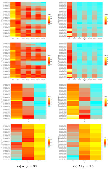
Figure 2.
Heatmap plots for the simulation (point/interval) results of .
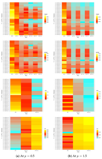
Figure 3.
Heatmap plots for the simulation (point/interval) results of .
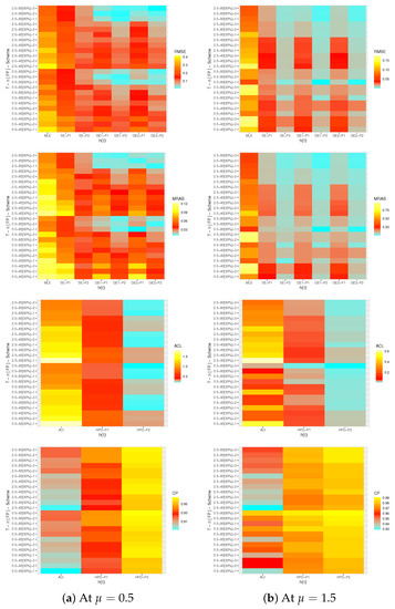
Figure 4.
Heatmap plots for the simulation (point/interval) results of .
- General comment is the proposed estimates of , or of the IL model in presence of T2-APHC sample behave well in terms of the lowest RMSE, MRAB and ACL values as well as the highest CP values.
- All Bayes point and interval estimates of , and , due to the gamma prior, perform well compared to the other estimates as expected. Similar result is also observed in the case of HPD intervals.
- Comparing the proposed priors 1 and 2, because the variance of prior-2 is lower than the variance of prior-1, it is noted that the Bayes calculations based on prior-2 have good perform for all unknown parameters than others.
- Asymmetric Bayes estimates of , or have overestimates (when ()) and have underestimates (when ()).
- As n(or m) increases, all estimates of , and perform satisfactory. A similar result is also observed when the sum of decreases.
- As increases, the RMSEs, MRABs and ACLs of increase while their CPs decrease as well as the RMSEs, MRABs and ACLs of and decrease while their CPs increase.
- As T increases, it can be seen that:
- (i)
- For
- -
- The simulated RMSE/MRAB values of the frequentist estimates of , and increase while that associated with the Bayes estimates of , and decrease.
- -
- The ACLs of ACI/HPD interval estimates of , and narrowed down while their CPs increase.
- (ii)
- For
- -
- The simulated RMSE/MRAB values of the both frequentist and Bayes estimates of , and decrease.
- -
- The ACLs of ACI/HPD interval estimates of decrease (with CPs increase) while of and increase (with CPs decrease).
- Comparing the proposed schemes 1, 2 and 3, it is noted that:
- (i)
- For
- -
- Under Scheme-3 (is also known right (or Type-II) censoring), all proposed point and interval estimates of behave better than others.
- -
- The same finding is also observed in the estimation results for and .
- (ii)
- For
- -
- The proposed point estimates of , and perform better for Scheme-1 (left-censoring) when and for Scheme-3 (right-censoring) when than others.
- -
- The proposed interval estimates of , and behave better under Scheme-3 (right-censoring) in most cases compared to others.
- As a recommendation, we propose to utilize the Bayes M-H algorithm procedure to estimate the IL parameters using T2-APHC.
5. Real-Life Applications
This section presents an analysis of two useful applications from the engineering and marketing fields to highlight the usefulness of the proposed estimation methods and the possibility of adapting study objectives to real practice.
5.1. Airborne Communication Transceiver
The airborne communication transceiver is a very high frequency and ultra-high frequency transceiver designed for communication between aircraft via the built-in intercom, in addition to communication with the ground means of air traffic control. In this application, we shall use a data set, reported by Jorgensen [26], consisting of forty observations of the active repair times (hours) for an airborne communication transceiver (ACT), see Table 1. In the past decade, this data set has received a lot of attention from several authors; for example, see Saroj et al. [27], Sharma et al. [28], Ferreira et al. [29], among others.

Table 1.
Times of active repair for ACT.
To explain the flexibility of the proposed model, based on the complete ACT data set, the IL distribution is compared to five other common inverted distributions (for and ) namely; inverse exponential (IE()) proposed by Keller et al. [30], inverse Weibull (IW()) proposed by Keller et al. [31], inverse gamma (IG()) discussed by Glen [32], inverted Nadarajah–Haghighi (INH()) proposed by Tahir et al. [33] and alpha power inverted exponential (APIE()) proposed by Ceren et al. [34] distributions. To determine which distribution has the best fit, different goodness-of-fit measures are considered called: negative log-likelihood (NL), Akaike (A), Bayesian (B), consistent Akaike (CA), Hannan-Quinn (HQ) and Kolmogorov–Smirnov (KS) statistic with its p-value. To calculate the proposed criteria, the MLE with its standard error (St.E) of or is calculated and presented in Table 2. It is evident, in terms of the smallest of NL, A, B, CA, HQ and KS values as well as the highest p-value, that the IL lifetime model provides a better fit than IE, IW, IG, INH and APIE distributions. For more investigation, the IL distribution is also compared to the Lindley (L) model. It is quite evident, from Table 2, that the IL distribution provides the best overall fit compared to L and other inverse models. Further, quantile-quantile plots of IL, IE, IW, IG, INH and APIE distributions are displayed in Figure 5. Furthermore, Figure 6 shows the histograms of ACT data and the lines of fitted densities as well as fitted/empirical reliability functions of IL, IE, IW, IG, INH and APIE distributions are displayed. It can be seen, from Figure 5 and Figure 6, that the IL distribution can be chosen as an appropriate distribution when compared to other distributions in presence of ACT data.
Table 2.
Fitting results of the IL and its competitive models from ACT data.
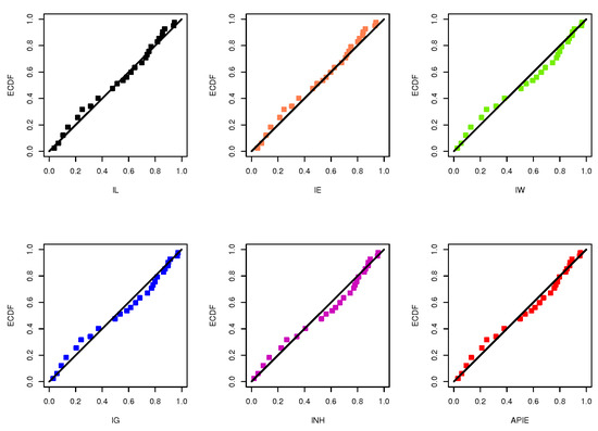
Figure 5.
The quantile-quantile plots of the IL and its competitive models from ACT data.
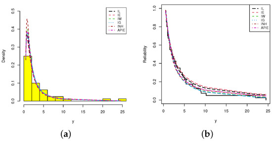
Figure 6.
(a) Histograms/Fitted PDFs; (b) Empirical/Fitted RFs from ACT data.
From the complete ACT data, when , three T2-APHC samples based on different schemes are generated and reported in Table 3. From Table 3, the MLEs with their St.Es of , and (at time ) are computed. By running the M-H algorithm 50,000 times with discarding the first 10,000 variates as burn-in, the Bayes estimates with their St.Es under SE and GE (for ) loss functions of , and are calculated using the improper gamma prior. Since there is no a priori information about from ACT data, we assume that the hyperparameters a and b are not available but are set to 0.001 to run computations. Also, the two bounds of the 95% ACI/HPD interval estimates with their lengths of the same parameters are also calculated. To apply the proposed MCMC sampler, the maximum likelihood estimate of is selected as an initial guess. The point and interval estimates of , and are provided in Table 4 and Table 5, respectively. It is clear, from Table 4 and Table 5, that the estimates of , and obtained by the MCMC procedure perform better than others. Similar performance is also observed in the case of HPD interval estimates.
Table 3.
Three generated samples from ACT data.
Table 4.
Point estimates (first-column) with their St.Es (second-column) of , and from ACT data.
Table 5.
Interval estimates of , and from ACT data.
Some common characteristics for the MCMC iterations of , and after burn-in, namely: mean, mode, quartiles (), standard deviation (St.D) and skewness are computed and provided in Table 6. To highlight the convergence of MCMC draws, from sample 1 (as an example), MCMC trace plots of , and are displayed in Figure 7. Additionally, using the fitted Gaussian kernel for sample 1, the histograms of MCMC variates of , and are also shown in Figure 7. For each trace plot, the sample mean is represented by a solid (—) line as well as the HPD interval bounds are represented by dashed (- - -) lines. For each histogram plot, the sample mean of each unknown parameter is represented with a vertical dotted (:) line. Figure 7 demonstrates that the MCMC sampler converges quite well and that the burn-in sample has a sufficient size to remove the effect of the starting values. It is also noted, from Figure 7, that the generated variates of , and are positive-skewed, negative-skewed and fairly symmetrical, respectively. Other trace and histogram plots of , and based on samples 2 and 3 are plotted and displayed in the Supplementary File.
Table 6.
Characteristics for MCMC outputs of , and from ACT data.
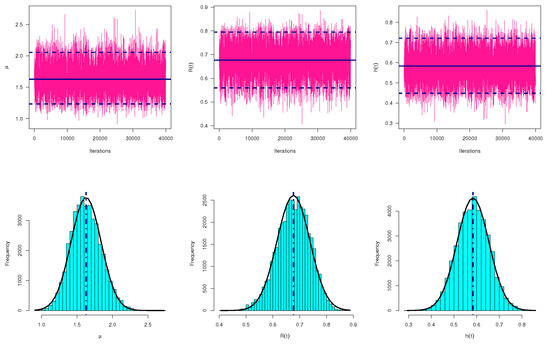
Figure 7.
Trace (top) and Histograms (bottom) plots of , and from ACT data.
5.2. Wooden Toys
In this application, from the marketing field, both proposed frequentist and Bayesian estimators of the IL parameters are computed based on the prices of the thirty different children’s wooden toys for sale at a Suffolk craft shop in April 1991, see Table 7. This data was originally published by The Open University and recently analyzed by Chesneau et al. [35]. In Table 8, the calculated values of NL, A, B, CA, HQ and KS(p-value) of IL and its competitive models are presented. It shows that the IL distribution fits the wooden toys data better compared to the Lindley model with respect to the KS(p-value) statistic alone. It is also evidence that the IL distribution is the best choice for the wooden toys data compared to other inverse models based on the criteria A, B, CA and HQ whereas the IW, IG, INH and APIE distributions are the next best-fit models based on the NL and KS(p-value) criteria.
Table 7.
Prices of wooden toys for sale at a Suffolk craft shop.
Table 8.
Fitting results of the IL and its competitive models from wooden toys data.
Also, using the complete wooden toys data, Figure 8 displays the quantile-quantile plots of IL, L, IE, IW, IG, INH and APIE distributions. It also supports the same findings reported in Table 8. Further, for each model based on the wooden toys data, the plot of histograms of wooden toys data with fitted densities as well as the plot of the fitted and empirical reliability functions are shown in Figure 9. It is evident that the IL distribution is the best model compared to its competitive models.
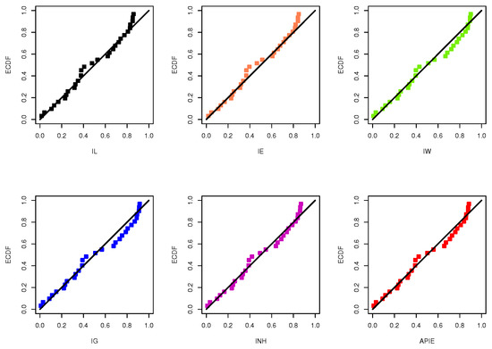
Figure 8.
The quantile-quantile plots of the IL and its competitive models from wooden toys data.
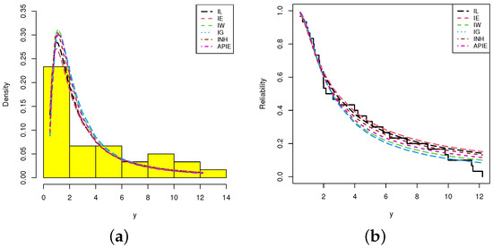
Figure 9.
(a) Histograms/Fitted PDFs; (b) Empirical/Fitted RFs from wooden toys data.
Now, we obtain the calculated values of the derived point and interval estimators of , and based on three different T2-APHC samples with size from the complete wooden toys data set which are listed in Table 9. From Table 9, the classical and Bayes MCMC estimates with their St.Es of , and (at time ) are computed and presented in Table 10. Moreover, two-sided 95% ACI/HPD interval estimates with their lengths of the same unknown quantities are also calculated, see Table 11. Utilizing the improper gamma prior under SE and GE (for ) loss functions, from 50,000 MCMC draws with 10,000 burn-in, the MCMC estimates with their St.Es of , and are developed. To run the desired computations, the hyperparameters a and b are selected to be 0.001. Moreover, the same properties mentioned in Table 6 are also reused based on the wooden toys data and reported in Table 12.
Table 9.
Three different samples from wooden toys data.
Table 10.
Point estimates (first-column) with their St.Es (second-column) of , and from wooden toys data.
Table 11.
Interval estimates of , and from wooden toys data.
Table 12.
Characteristics for MCMC outputs of , and from wooden toys data.
It is observed, from Table 10 and Table 11, that the fitted values of the point and interval estimators of , and derived from the Bayes paradigm performed better than those derived from the likelihood approach in terms of the lowest St.Es, as well as, the HPD interval estimates are also performed better than others in terms of the shortest intervals. Using the data set of sample 1 as an example, both trace and histogram plots of the MCMC variates of , and are provided in Figure 10. It shows that the MCMC mechanism converges well and demonstrates that the MCMC variates of and are fairly symmetrical while that associated with are positive-skewed. Other plots of , and based on samples 2 and 3 are presented in the Supplementary File. Finally, from both engineering and marketing examples, we can conclude that the proposed methodologies provide a satisfactory interpretation of the IL lifetime model in presence of a sample obtained from an adaptive Type-II progressive hybrid censoring mechanism.
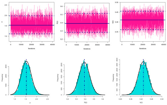
Figure 10.
Trace (top) and Histograms (bottom) plots of , and from wooden toys data.
6. Concluding Remarks
This study takes into account the statistical inference of the unknown parameter and some reliability measures of the inverse Lindley distribution using adaptive Type-II progressively censored samples. The various parameters are inferred using both conventional and Bayesian methods. We employ numerical techniques to acquire the necessary estimate of the unknown parameter because it has been shown that its estimator cannot be derived in closed form. The asymptotic properties of the maximum likelihood estimators are used to produce the approximate confidence intervals in addition to the point estimates of the unknown parameter, reliability, and hazard rate functions. We study the Bayesian estimation of various unknown parameters using symmetric and asymmetric loss functions, and it is noted that they cannot be obtained in closed expressions because of the complexity of the posterior distribution. In order to get the Bayes point estimates and the highest posterior density credible intervals, the Markov chain Monte Carlo method was applied. Various statistical criteria, including root mean squared error and interval length, were assessed using Monte Carlo simulations to determine the performance of the proposed methods. The suggested approaches are demonstrated through two examples involving real data sets. According to the numerical outcomes, the Bayes estimates are more precise than maximum likelihood estimates in terms of minimum root mean squared error, relative absolute bias, and interval length. As the number of observed failures increases the different estimation methods perform well for the different progressive censoring schemes. As the variance of the prior distribution decreases, the Bayes estimates perform well when compared with those with high variance. Furthermore, the Bayes estimates using the general entropy loss function as asymmetric loss function are more efficient than estimates obtained based on the symmetric squared error loss function. Finally, the analysis of two data sets shows that the inverse Lindley distribution can be used as a suitable model when compared with some other competitive models, including Lindley, inverse Weibull and inverted Nadarajah–Haghighi distributions. As a future work, it is of interest to investigate other estimation methods like maximum product of spacing and expectation-maximization algorithm of the inverse Lindley distribution using the same censoring scheme.
Supplementary Materials
The following supporting information can be downloaded at: https://www.mdpi.com/article/10.3390/axioms12050427/s1. Table S1: The AEs (1st column), RMSEs (2nd column) and MRABs (3rd column) of when ; Table S2: The AEs (1st column), RMSEs (2nd column) and MRABs (3rd column) of when ; Table S3: The AEs (1st column), RMSEs (2nd column) and MRABs (3rd column) of when ; Table S4: The AEs (1st column), RMSEs (2nd column) and MRABs (3rd column) of when ; Table S5: The AEs (1st column), RMSEs (2nd column) and MRABs (3rd column) of when ; Table S6: The AEs (1st column), RMSEs (2nd column) and MRABs (3rd column) of when ; Table S7: The ACLs (1st column) and CPs (2nd column) of ACI/HPD credible intervals of ; Table S8: The ACLs (1st column) and CPs (2nd column) of ACI/HPD credible intervals of ; Table S9: The ACLs (1st column) and CPs (2nd column) of ACI/HPD credible intervals of ; Figure S1: Trace (top) and Histograms (bottom) plots of , and under sample 2 from ACT data; Figure S2: Trace (top) and Histograms (bottom) plots of , and under sample 3 from ACT data; Figure S3: Trace (top) and Histograms (bottom) plots of , and under sample 2 from wooden toys data; Figure S4: Trace (top) and Histograms (bottom) plots of , and under sample 3 from wooden toys data.
Author Contributions
Methodology, A.E. & M.N.; validation R.A.; Funding acquisition, R.A.; Software, A.E.; resources R.A.; Supervision A.E.; Writing—original draft, R.A. & M.N.; formal analysis M.N.& R.A.; Writing—review & editing M.N. All authors have read and agreed to the published version of the manuscript.
Funding
This research was funded by Princess Nourah bint Abdulrahman University Researchers Supporting Project number (PNURSP2023R50), Princess Nourah bint Abdulrahman University, Riyadh, Saudi Arabia.
Data Availability Statement
The authors confirm that the data supporting the findings of this study are available within the article.
Acknowledgments
The authors would also like to express their gratitude to the Editor-in-Chief and anonymous referees for their constructive comments and suggestions, which significantly improved the paper. Princess Nourah bint Abdulrahman University Researchers Supporting Project number (PNURSP2023R50), Princess Nourah bint Abdulrahman University, Riyadh, Saudi Arabia.
Conflicts of Interest
The authors declare no conflict of interest.
References
- Lindley, D.V. Fiducial distributions and Bayes’ theorem. J. R. Stat. Soc. Ser. (Methodol.) 1958, 20, 102–107. [Google Scholar] [CrossRef]
- Sharma, V.K.; Singh, S.K.; Singh, U.; Agiwal, V. The inverse Lindley distribution: A stress-strength reliability model with application to head and neck cancer data. J. Ind. Prod. Eng. 2015, 32, 162–173. [Google Scholar] [CrossRef]
- Basu, S.; Singh, S.K.; Singh, U. Parameter estimation of inverse Lindley distribution for Type-I censored data. Comput. Stat. 2017, 32, 367–385. [Google Scholar] [CrossRef]
- Basu, S.; Singh, S.K.; Singh, U. Bayesian inference using product of spacings function for Progressive hybrid Type-I censoring scheme. Statistics 2018, 52, 345–363. [Google Scholar] [CrossRef]
- Basu, S.; Singh, S.K.; Singh, U. Estimation of inverse Lindley distribution using product of spacings function for hybrid censored data. Methodol. Comput. Appl. Probab. 2019, 21, 1377–1394. [Google Scholar] [CrossRef]
- Hassan, M.K.; Alohali, M.I.; Alojail, F.A. A new application of R= P [Y< X] for the inverse Lindley distribution using ranked set sampling. J. Stat. Manag. Syst. 2021, 24, 1713–1731. [Google Scholar]
- Ng, H.K.T.; Kundu, D.; Chan, P.S. Statistical analysis of exponential lifetimes under an adaptive Type-II progressive censoring scheme. Nav. Res. Logist. 2009, 56, 687–698. [Google Scholar] [CrossRef]
- Al Sobhi, M.M.A.; Soliman, A.A. Estimation for the exponentiated Weibull model with adaptive Type-II progressive censored schemes. Appl. Math. Model. 2016, 40, 1180–1192. [Google Scholar] [CrossRef]
- Hemmati, F.; Khorram, E. On adaptive progressively Type-II censored competing risks data. Commun. Stat. Simul. Comput. 2017, 46, 4671–4693. [Google Scholar] [CrossRef]
- Nassar, M.; Abo-Kasem, O.; Zhang, C.; Dey, S. Analysis of Weibull distribution under adaptive Type-II progressive hybrid censoring scheme. J. Indian Soc. Probab. Stat. 2018, 19, 25–65. [Google Scholar] [CrossRef]
- Panahi, H.; Moradi, N. Estimation of the inverted exponentiated Rayleigh distribution based on adaptive Type II progressive hybrid censored sample. J. Comput. Appl. Math. 2020, 364, 112345. [Google Scholar] [CrossRef]
- Elshahhat, A.; Nassar, M. Bayesian survival analysis for adaptive Type-II progressive hybrid censored Hjorth data. Comput. Stat. 2021, 36, 1965–1990. [Google Scholar] [CrossRef]
- Panahi, H.; Asadi, S. On adaptive progressive hybrid censored Burr type III distribution: Application to the nano droplet dispersion data. Qual. Technol. Quant. Manag. 2021, 18, 179–201. [Google Scholar] [CrossRef]
- Du, Y.; Gui, W. Statistical inference of adaptive type II progressive hybrid censored data with dependent competing risks under bivariate exponential distribution. J. Appl. Stat. 2022, 49, 3120–3140. [Google Scholar] [CrossRef] [PubMed]
- Alotaibi, R.; Nassar, M.; Elshahhat, A. Computational Analysis of XLindley Parameters Using Adaptive Type-II Progressive Hybrid Censoring with Applications in Chemical Engineering. Mathematics 2022, 10, 3355. [Google Scholar] [CrossRef]
- Alotaibi, R.; Elshahhat, A.; Rezk, H.; Nassar, M. Inferences for Alpha Power Exponential Distribution Using Adaptive Progressively Type-II Hybrid Censored Data with Applications. Symmetry 2022, 14, 651. [Google Scholar] [CrossRef]
- Ateya, S.F.; Amein, M.M.; Mohammed, H.S. Prediction under an adaptive progressive type-II censoring scheme for Burr Type-XII distribution. Commun. Stat. Theory Methods 2022, 51, 4029–4041. [Google Scholar] [CrossRef]
- Elshahhat, A.; Nassar, M. Analysis of adaptive Type-II progressively hybrid censoring with binomial removals. J. Stat. Comput. Simul. 2022. [Google Scholar] [CrossRef]
- Greene, W.H. Econometric Analysis, 4th ed.; Prentice-Hall: New York, NY, USA, 2000. [Google Scholar]
- Calabria, R.; Pulcini, G. An engineering approach to Bayes estimation for the Weibull distribution. Microelectron. Reliab. 1994, 34, 789–802. [Google Scholar] [CrossRef]
- Gelman, A.; Carlin, J.B.; Stern, H.S.; Rubin, D.B. Bayesian Data Analysis, 2nd ed.; Chapman and Hall/CRC: Boca Raton, FL, USA, 2004. [Google Scholar]
- Lynch, S.M. Introduction to Applied Bayesian Statistics and Estimation for Social Scientists; Springer: New York, NY, USA, 2007. [Google Scholar]
- Chen, M.H.; Shao, Q.M. Monte Carlo estimation of Bayesian credible and HPD intervals. J. Comput. Graph. Stat. 1999, 8, 69–92. [Google Scholar]
- Henningsen, A.; Toomet, O. maxLik: A package for maximum likelihood estimation in R. Comput. Stat. 2011, 26, 443–458. [Google Scholar] [CrossRef]
- Plummer, M.; Best, N.; Cowles, K.; Vines, K. CODA: Convergence diagnosis and output analysis for MCMC. R News 2006, 6, 7–11. [Google Scholar]
- Jorgensen, B. Statistical Properties of the Generalized Inverse Gaussian Distribution; Springer: New York, NY, USA, 1982. [Google Scholar]
- Saroj, A.; Sonker, P.K.; Kumar, M. Statistical properties and application of a transformed lifetime distribution: Inverse muth distribution. Reliab. Theory Appl. 2022, 17, 178–193. [Google Scholar]
- Sharma, V.K.; Shekhawat, K.; Chesneau, C. On Generating Families of Power Quantile Distributions for Modeling Waiting and Repair Times Data. J. Indian Soc. Probab. Stat. 2021, 22, 155–179. [Google Scholar] [CrossRef]
- Ferreira, P.H.; Ramos, E.; Ramos, P.L.; Gonzales, J.F.; Tomazella, V.L.; Ehlers, R.S.; Silva, E.B.; Louzada, F. Objective Bayesian analysis for the Lomax distribution. Stat. Probab. Lett. 2020, 159, 108677. [Google Scholar] [CrossRef]
- Keller, A.Z.; Kamath, A.R.R.; Perera, U.D. Reliability analysis of CNC machine tools. Reliab. Eng. 1982, 3, 449–473. [Google Scholar] [CrossRef]
- Keller, A.Z.; Goblin, M.T.; Farnworth, N.R. Reliability analysis of commercial vehicle engines. Reliab. Eng. 1985, 10, 15–25. [Google Scholar] [CrossRef]
- Glen, A. On the inverse gamma as a survival distribution. J. Qual. Technol. 2011, 43, 158–166. [Google Scholar] [CrossRef]
- Tahir, M.H.; Cordeiro, G.M.; Ali, S.; Dey, S.; Manzoor, A. The inverted Nadarajah–Haghighi distribution: Estimation methods and applications. J. Stat. Comput. Simul. 2018, 88, 2775–2798. [Google Scholar] [CrossRef]
- Ceren, Ü.; Cakmakyapan, S.; Gamze, Ö. Alpha power inverted exponential distribution: Properties and application. Gazi Univ. J. Sci. 2018, 31, 954–965. [Google Scholar]
- Chesneau, C.; Tomy, L.; Gillariose, J.; Jamal, F. The inverted modified Lindley distribution. J. Stat. Theory Pract. 2020, 14, 1–17. [Google Scholar] [CrossRef]


Disclaimer/Publisher’s Note: The statements, opinions and data contained in all publications are solely those of the individual author(s) and contributor(s) and not of MDPI and/or the editor(s). MDPI and/or the editor(s) disclaim responsibility for any injury to people or property resulting from any ideas, methods, instructions or products referred to in the content. |
© 2023 by the authors. Licensee MDPI, Basel, Switzerland. This article is an open access article distributed under the terms and conditions of the Creative Commons Attribution (CC BY) license (https://creativecommons.org/licenses/by/4.0/).