Abstract
This paper reports a study to interpret the surface temperature based on time series and fuzzy measures. We demonstrated a method to identify the uncertainty around the surface temperature data concerning the summer monsoon in India. The random variables were standardized, and the Dempster-Shafer Theory was used to generate common goals. Two criteria, represented as fuzzy numbers, were used for this purpose. We constructed three polynomials to illustrate a functional connection between time series and the measure of joint belief. The analysis of the obtained results showed that the certainty increased over time. It confirmed that the degree of the evidence is a more predictable parameter at a more extended period.
Keywords:
Dempster-Shafer Theory; fuzzy set; joint belief measure; northeast India; surface temperature MSC:
62M10; 94A15
1. Introduction
Back in the 1980s, Zadeh published a pioneering article that showed how the Dempster-Shafer Theory (DST) of evidence had enormous potential for the A.I. field in dealing with uncertainty in expert systems [1]. The relational method facilitates the Dempster-Shafer theory’s applicability in AI-related applications and resolves some of its issues. According to Zadeh, the DST can be viewed as applying traditional retrieval techniques to second-order relations in first normal form in relational databases. To optimize the resulting flood susceptibility maps based on some flood conditioning elements, [2] worked on the flood susceptibility maps for the Austrian region of Salzburg using several models supplemented by DST. An extension of the Bayesian theory of subjective probability is the idea of belief functions, also known as the DST [3,4,5,6,7]. Belief functions enable us to construct degrees of belief for one question based on probabilities for another instead of the Bayesian theory’s [8,9,10,11,12,13,14] requirement for probabilities for each relevant question. Depending on how closely the two issues are linked, these degrees of belief may or may not possess the mathematical properties of probability. In a different study, reference [15] showed how incorporating DST into investigating landslide susceptibility across Austria could enhance the findings. Reference [16] demonstrated a fuzzy-based flood analysis of urban drainage systems. They [16] reported a probabilistic structure of rainfall characteristics and discussed fuzzy model parameters through a probabilistic representation of random variables and a fuzzy representation of model parameters for flood analysis. The uncertainty associated with severity probabilities of flood quantities was examined in a unified DST model that combined a probabilistic representation of rainfall uncertainty with a fuzzy representation of model parameters. To identify aquifer sensitivity zones for nitrate contamination in the Galal Badra basin, east of Iraq, the reference [17] used the DST of evidence in a GIS system.
Although Dempster and Shafer carried out the studies that gave rise to the Dempster-Shafer theory, its primary logic goes back to the seventeenth century [18,19]. When artificial intelligence (A.I.) researchers sought a way to apply probability theory to expert systems in the early 1980s [20,21], they stumbled across this theory. Further study has shown that handling uncertainty requires more structure than is available in simple rule-based systems. However, the DST still has value because of its relative flexibility [22]. The DST [23] is based on using a related topic’s subjective probability to generate degrees of belief for a separate issue and applying Dempster’s rule to combine those degrees of belief when independent pieces of evidence support them. Generally, probabilities for one topic are used to calculate degrees of belief for another. Beginning with the idea that the questions for which we have probabilities are independent concerning our subjective probability judgments, Dempster’s rule says that this independence is only an a priori property that disappears once the conflict between the different pieces of evidence is found. One must resolve two related problems before applying the DST to a particular problem. To start, we must group the uncertainties in the issue into a priori independent pieces of evidence. Second, we need to use computation to implement Dempster’s rule. The solutions to these two problems are linked together. A structure incorporating evidence pertinent to various but related questions is produced by breaking down the uncertainties into their parts and can be used to make computations possible. The work of Dempster on probabilities with upper and lower limits serves as the foundation for the D.S. approaches. Since then, they have become widely accepted in the expert systems and A.I. literature, emphasizing incorporating data from various sources. This work presents the basic concepts of the DST of evidence and a short discussion of its historical background and similarities to the more traditional Bayesian theory [24,25]. After that, they discussed current developments in this theory and pertinent analytical and application subjects. North East India (NEI), which consists of eight states, is highly susceptible to environmental shifts. In this study, the actual observations made at the meteorological stations of the India Meteorological Department (IMD) in the area and on the gridded data are used to analyze the current climatic conditions that are present in NEI. In order to investigate the trends and potential impacts of global warming, a new comprehensive surface temperature data set for India is used to chart temperature changes for seven decades. The data set is divided into three categories for investigating the temperature patterns during each of these times: pre-monsoon, summer monsoon, and post-monsoon. Global warming has become a source of worry for meteorologists over the past few decades. [26] discovered the Kothawale and Weakened Seasonal Asymmetry of Trends in Temperature, which has been interpreted as the result of a rise in temperature during the monsoon. [27] A very recent study examined the multi-decadal patterns of surface temperature change over India. They found that northwest and southern India warmed while northeastern and southwest India cooled. It is well-known how crucial it is to examine atmospheric temperature at various stages [28,29,30]. Reference [28] demonstrated a decrease in the minimum temperature during the summer monsoon over India and reported an increase during post-monsoon months. They [28] have shown how a significant difference in seasonal temperature anomalies might bring about seasonal asymmetry and changes in atmospheric circulation. Reference [29] reported that although there are day-to-day fluctuations of pre-monsoon daily maximum and minimum temperatures over some meteorological regions of India, there is no significant change in the day-to-day magnitude of fluctuations of pre-monsoon maximum and minimum temperatures. Reference [30] performed a spatial and temporal trend analysis of both minimum and maximum temperature time series in different scales. After a trend detection analysis through various non-parametric methods taking serial correlation into account, they [30] exercised a sequential Mann-Kendal test to reveal the trend pattern at annual or seasonal levels. Reference [31] presented a modeling system to predict both internal variability and externally forced changes in surface temperature on regional and global scales. They [31] emphasized the necessity of attempting to predict internally generated natural temperature variability apart from natural and anthropogenic sources. In sharp contrast to model simulations, reference [32] reported that global-mean surface temperature has shown no discernible warming despite a steady increase in atmospheric greenhouse gases since about 2000. Reference [33] reported the effect of inter annual variations in vegetation within land covers on surface temperature in North America and Eurasia using statistical techniques on satellite data. Reference [34] reported a two-state Markov chain approach and an autoregressive approach to study the surface temperature time series over northeast India. It [34] concluded that the autoregressive model of order two best represents the average monthly time series of surface temperatures over northeast India. In reference [35], the timing of climate change reaction is revealed by the relative phasing of temperature versus forcing mechanisms. References [35,36,37] demonstrated the importance of surface temperature in urban climate modeling.
Before going into further details of the study, let us emphasize the newness of the approach and outcomes. We have focused on interpreting the surface temperature based on time series and fuzzy measures. In the subsequent sections, we will present a method to identify the uncertainty around the surface temperature data concerning the summer monsoon in India. The random variables will be standardized, and we will use the DST to generate common goals. For this purpose, we will use two criteria, represented as fuzzy numbers. We will present three polynomials to illustrate a functional connection between time series and the measure of joint belief. The aroma of the newness of the present study lies in the fact that instead of presenting the conventional statistical methodology, we will explore the uncertainty associated with the data through DST, wherein we will consider two separate queries on the same universe of discourse and will find the join belief measure to find the combined belief measure through Dempster’s rule of combination.
Organization of the remaining part of the paper is as follows: In Section 2, we have described the study area and data to be used, belief measure and Dempster-Shafer theory. In Section 3 we have demonstrated the outcomes of the study in the form of results and discussions and we have concluded in Section 4.
2. Study Area, Data Used, and Methodology
The study was conducted in North East India (NEI), located in the Eastern Himalayan region. Its perimeter is defined by latitudes 21°08′ to 30°12′ N and longitudes 87°50′ to 96°30′ W. The Brahmaputra Basin is part of this area, which experiences heavy rains. Due to distinct attributes, including orography, alternating pressure cells over NEI and the Bay of Bengal, and the local mountain and valley winds, the climate of NEI differs from that of the rest of India. The big water bodies and forested areas further enhance its unique climate. NEI is covered by meteorological subdivisions (a) Arunachal Pradesh, (b) Assam and Meghalaya, (c) Nagaland, Manipur, Mizoram, and Tripura defined by India Meteorological Department (IMD). Please see the map in Figure 1.
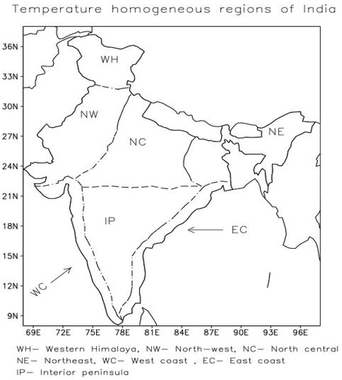
Figure 1.
A Map of the Temperature homogeneous regions of India were taken from https://www.tropmet.res.in/data/data-archival/txtn/TEMP-REG.jpg (accessed on 25 April 2023).
The observational data on surface temperature over Northeast India from 1901–2007 are collected from the website of the Indian Institute of Tropical Meteorology (IITM). The link to the data is https://tropmet.res.in/static_pages.php?page_id=54 (accessed on 25 April 2023).
Fuzzy measure theory, as comprehensively defined in [38], provides us with a broad framework to introduce and investigate possibility theory. This topic is closely related to fuzzy set theory [39] and is crucial in several applications. Certain conditions must be met by the function h for fuzzy measures to be categorized. In the past, these vital components were believed to be found in the fundamental principles of probability theory, but this assumption needed to be corrected. Since weaker assumptions define them, probability measures are a particular form of fuzzy measure. The following are the principles of fuzzy measures:
- For every if then
- For every sequence of subsets of , if either or (i.e., the sequence is monotonic), then
A belief measure is defined by a function , Which satisfies the axioms of fuzzy measures and another additional axiom defined as follows:
For every and every collection of subsets of .
Every belief measure and its dual plausibility measure can be expressed as a function.
Such that and
where m(A) indicates the degree of the evidence for the claim that a particular member of X belongs to the set A but not to any subset of A, or how strongly we think the evidence supports this claim.
Dempster-Shafer theory (DST) is a generalized method for describing uncertainty [40]. This theory is defined as an extension of probability theory. The Dempster-Shafer theory is named after works by A. P. Dempster and Glenn Shafer, but the thinking it employs dates back to the seventeenth century. Instead of single propositions, it comprises collections of prepositions, and each set is given an interval within which the degree of belief must fall. To allow a degree of belief, the DST has been established, and it is known as a theory of evidence because it works with the weight of the evidence. We consider , a set of n exhaustive and mutually exclusive propositions, where 0 is referred to as a context of judgement. Thus, the Boolean operator OR can be used to create propositions; is the collection of all subsets of 0. Dempster-Shafer introduced the idea of mass probability, denoted as , to assign evidence to a proposition where Y is the Universe of discourse
Mass probability can also be termed a basic probability assignment (bpa). The support is the total degree of belief that is to be true for a hypothesis. So, a belief function can be defined as
where denotes the degree of support for the hypotheses of , then the multiple hypotheses become
A belief function’s characteristics are as follows:
Non-beliefs are defined as any belief unrelated to a particular subset and associated with the symbol . In general, a belief function is written as bpa. Conventionally, means that the mass probability of the empty set is zero.
Using the Dempster formula of combination, data association is carried out using the Dempster-Shafer theory. It can be explained as follows:
The orthogonal sum of and is used to describe the sum of the mass product intersections and total belief of is defined as:
The above-mentioned methodology would be applied in Section 3.
The procedural flow of the work to be presented in the subsequent section is summarized in the following steps:
- As the first step, the data are scaled to [0, 1];
- Considering two measures of central tendency, two fuzzy sets are created;
- Considering the two measures of central tendencies as two judging criteria, different focal elements are generated based on α-cuts;
- Measures of combined belief are computed for different focal elements according to DST;
- Three polynomials are created as a functional relationship between the time scale and the measure of joint belief;
- Varying the leading coefficients over a range of values, we have generated 3-dimensional surfaces to interpret the association between belief measure and time scale.
3. Results and Discussions
This section analyses the surface temperature data during the summer monsoon (JJAS) in North East India from 1901 to 2007. All the values have been standardized. In the following stage, we considered a universe of discourse for the summer monsoon (JJAS) and computed the mean and median to produce a fuzzy set that is “close to the mean and median respectively”. The following transformation is used to scale the data so that its values fall between 0 and 1 if x represents the realization of the time series at a certain time point:
where the suffix i denotes realization at the i-th time point. A fuzzy set has been created whose elements are drawn from the time series as members of a crisp set and whose membership function is given by
In order to calculate the joint belief, c will be taken into consideration as the mean and median for the two judging criteria.
The methodology mentioned in the previous section is now being applied in this final stage. In the first scenario, we considered two basic assignments, , and , for the summer monsoon (JJAS) for 107 years, where and stand for basic assignments for mean and median, respectively. Then, three focal elements R, D, and C were taken into consideration, each of which represented a fuzzy set “very close” to the mean or median, “close” to the mean or median, and “moderately close” to the mean or median, respectively. Furthermore, we calculated R, D, C, as well as the unions of all the focus elements, i.e., R D, R C, D C, and R D C, which are assigned with the membership grades derived from the various α- cuts. For each focal element, we have determined the joint belief, or “” by applying Dempster’s rule to and .
Again, we created two data sets for the summer monsoon (JJAS) spanning 50 years each. We determined the focal elements R, D, and C and the unions of all the focal elements. Then we gave membership grades to each element based on the various α- cuts. Using Dempster’s method to the basic assignments and for each focal element, we determined the joint belief, or .
By using four sets of time periods, each including data for 25 years, we determined the joint belief and basic assignments for all the focal elements of summer monsoon (JJAS).
We have demonstrated joint belief for JJAS in Table 1, with the basic probability assignments based on the fuzzy sets of surface temperature amounts close to mean and median, respectively. The joint beliefs of the window sizes of 50 and 25 are presented in Table 2 and Table 3 respectively. Assuming there are two judges to evaluate the system, one will think that the surface temperature value is relative to the mean, while the other will consider that it is close to the median. Since all the elements in the first column have basic probability assignments that are non-zero, they can all be considered focal elements. The joint belief is presented as the combined evidence in the fourth column of each table. We may conclude that for JJAS, most of the monthly surface temperature values are near the mean and median because it is observed that the joint belief for R D and R C has the highest joint belief measure. However, none of the joint beliefs are larger than or equal to 0.5 according to the combined bodies of evidence. Therefore, we comprehend that although perfect symmetry is unavailable for JJAS, the data are close to symmetry. This suggests that the 107-year time series of JJAS surface temperature data over northeast India deviates from symmetry and contains some degrees of uncertainty.

Table 1.
The values of joint belief for the four focal elements derived from surface temperature data corresponding to JJAS corresponding to 1901–2000.
Table 2.
The values of joint belief for the four focal elements derived from surface temperature data corresponding to JJAS data broken into windows of 50 years (1901–1950 and 1951–2000).
Table 3.
The measures of joint belief for the four focal elements derived from surface temperature data corresponding to JJAS data broken into windows of 25 years (1901–1925, 1926–1950, 1951–1975 and 1976–2000).
In the next part, we have divided the time series previously mentioned into 50-year segments for our study. We have considered the first and second 50 years for JJAS in Table 2a,b. The joint belief measures for the first two focal components are above 0.50, according to Table 2a for JJAS. Joint belief measures for the first two focal elements show strong evidence favoring to be around mean and median, which suggests a substantial body of evidence. This implies that the mean and median are very close and that the combined body of evidence firmly supports the data indicating that the mean and median are close. The joint body of data has a belief measure of less than 0.50 for the first two elements for the subsequent 50 years. Please note that while computing the mean and median, we consider the data set of 1901–2007. However, as we constructed the focal elements in different time scales, the data from 2001 to 2007 were not used because the time scales were multiples of 5. Because of this, although the data are almost symmetric, absolute symmetry is not accessible.
In the following research stage, we divided the time series into 25-year segments and computed the joint belief measure for each duration window. We found that the joint belief was declining.
In the final part of the work, we created three polynomials as a functional relationship between the time scale and the measure of joint belief where the belief measure is considered to be an independent variable, and it can be written in the form:
In this case, y is a timescale, and z is a joint belief measure. Subsequently, all real coefficients have generated polynomials of degrees 3, 4 and 5. None of the polynomials appeared to be monic. Hence, we have the leading coefficient not equal to 1. Varying the leading coefficients over a range of values we have generated a 3-dimensional surface in each case (please see Figure 2a–c). In Figure 2a we observed that the surface has an upward pattern with a time scale.
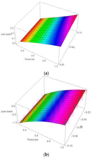
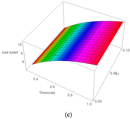
Figure 2.
Diagrams (first-panel (a), second-panel (b), third-panel (c)) illustrating the evolution of the joint belief measure over time for the surface temperature of JJAS.
Furthermore, the inclination is steeper in the case of higher values of the leading coefficient. A similar pattern is observed in a polynomial of degree 4 (see Figure 2b). However, in the case of a polynomial of degree 5, the surface gets curved (see Figure 2c), and we observed that the curvature is not affected by the change in the leading coefficient.
Contrary to the pattern available for rainfall [41] the surface is not getting a full convex pattern around any time scale. This indicates that we change in the time scale; the joint belief measure has a regular tendency to increase. The degree of evidence is getting stronger with the time scale. Hence the predictability of this climate parameter is less for lower time scales and more for higher time scales. This indicates the necessity of nonlinear methodologies for predicting climate parameters in a shorter time frame.
4. Conclusions
In the present paper, we have reported an application of the Dempster-Shafer theory to interpret the surface temperature time series over a meteorological subdivision of India. In this theory, evidence obtained in the same context but from two independent sources in a similar field of inquiry is combined and expressed through two basic assignments in the form of a joint basic assignment. In this context, for every subset in the power set of some universe of discourse, the belief measure is interpreted as the degree of belief based on available evidence. The essence of the theory is that one can view the subsets of the body of evidence as answers to a particular query. We assume that some of the answers are correct, but we need to identify the correct ones fully. Equation (1) about belief measures implies the monotonicity axiom of fuzzy measures.
We have created a methodology in the study described in the previous section to comprehend the uncertainty related to the summer monsoon’s (JJAS) surface temperature over Northeast India for the years 1901–2007. After standardizing all the values, we moved on to the next step, where we considered the Universe of discourse for the summer monsoon (JJAS) and calculated the mean and median to create a fuzzy set that represented the crisp set’s elements as being “close to the mean and median respectively.” Then, to compute the joint belief measure using the Dempster-Shafer Theory, we have considered two basic assignments, , and , for the summer monsoon (JJAS) for 107 years. and are the basic assignments corresponding to the consideration of mean and median, respectively. Then, three focal elements, R, D, and C, which, respectively, stand for fuzzy sets “very close” to mean/median, “close” to mean/median, and “moderately close” to mean/median, have been taken into consideration.
Furthermore, we have determined R, D, C, and the unions of all focus components, i.e., R D, R C, D C, and R D C, assigned with the membership grades derived from the various α-cuts. We have determined the joint belief, or “” for each focal element by applying Dempster’s method to and . Following a thorough investigation using the Dempster-Shafer method, we have found that uncertainty rises as we examine the time series of smaller windows rather than the entire time series. Finally, using a second-degree polynomial to represent the functional relationship between the time scale and the joint belief measure, we described the association using three-dimensional plots, revealing how the joint belief measure changed as the window size and leading coefficient of the polynomial that represented the relationship between them changed. The figures (Figure 2) show that the surfaces represent the joint belief measure. In each instance, a 3-dimensional structure was produced by varying the leading coefficients over a range of values. We can see that the surface in Figure 2a has an upward design with a time scale.
Additionally, the inclination is sharper when the leading coefficient has larger values. A comparable pattern is seen in the case of degree 4 polynomials. However, when a polynomial of degree 5 is involved, the surface curves, and we found that the curvature is unaffected by a shift in the leading coefficient. This shows that the joint belief measure consistently grows as time goes on. The strength of the evidence increases over time. Because of this, the predictability of this climate indicator is better at longer time scales than at shorter time scales. Finally, we understand that nonlinear methodologies are essential for forecasting the climate parameter in a shorter period. In future research, we want to expand this strategy to a multivariate framework that considers additional climatological factors that affect surface temperature over the study zone.
Long back, McBratney and Moore (1985) [42] implemented the fuzzy sets approach as a realistic and flexible one to information transfer than classifying climate into discrete sets. In due course, McBratney and Odeh (1997) [43] described fuzzy systems, including fuzzy set theory and fuzzy logic, as a potential tool to significantly improve or extend conventional logic and demonstrate phenomena associated with soil through it. Another important work in meteorology is Luydmila et al. (2017) [44], where the authors proposed a fuzzy-logic-based model for agro-meteorological modeling. The current approach differs from the earlier ones. Instead of fuzzy logic, we have reported a fuzzy-set theoretic approach to represent a functional connection between time series and the measure of joint belief through DST. The purpose is not precisely prediction but to give insight into the time series and analysis of the obtained results proving that the certainty increased over time. The study also confirmed that the degree of the evidence is a more predictable parameter over a more extended period. While conclusion, let us comment on the relative advantages of the methodology over the existing and conventional ones. In the references mentioned throughout the text, the focus has mainly been on predicting or studying the trend of the time series. However, in the current work, the primary focus has been exploring the time series’ intrinsic fuzziness through joint belief measures. This measure is through DST; before that, we generated fuzzy sets, and through alpha-cuts, we built focal elements required for constructing the joint belief function. In this context, let us compare the current procedure with another work where one of the present authors has quantified the uncertainty through Shannon entropy (Saha and Chattopadhyay, 2020) [45]. This work shows how entropy is affected by the fluctuation of mean rainfall on seasonal and yearly scales.
Contrary to the study of [45], the current work has explored the possibility of DST to probe the intrinsic uncertainty associated with a climatological parameter. Although the basic procedure of the present study differs from the work [45], the flexibility of both approaches is noteworthy. Prediction of climatological time series through artificial neural networks, an essential component of soft computing techniques, was reported in [46]. This procedure’s advantage lies in the flexibility of the approach attributed to the fuzzy set theory, a generalization of crisp set theory. Also, let us comment on the future direction of the current work. In this work, we have confined ourselves to a univariate scenario. We propose extending the approach to a multivariate framework by considering other climatological parameters. We offer to assess the correlation between relevant climatological parameters through a fuzzy-set theoretic approach in variable time scales. Through this, we expect to move towards extending this kind of DST-based approach to a broader perspective of the multivariate climatological forecast.
Author Contributions
R.R.D. and S.C. jointly framed the problem. R.R.D. has done the computational part with mentoring from S.C. R.R.D. has made the development of the text. The two authors have jointly interpreted. Both authors have contributed equally to the preparation of the final draft. All authors have read and agreed to the published version of the manuscript.
Funding
This research received no external funding.
Data Availability Statement
The data utilized in work are taken from the Indian Institute of Tropical Meteorology website (IITM). https://tropmet.res.in/static_pages.php?page_id=54 (accessed on 25 April 2023) is the link to the data. Furthermore, in the Figure 1 map of the Temperature homogeneous regions of India was taken from https://www.tropmet.res.in/data/data-archival/txtn/TEMP-REG.jpg (accessed on 25 April 2023).
Acknowledgments
The authors acknowledge the insightful comments from the reviewers with gratitude. The data utilized in work are taken from the Indian Institute of Tropical Meteorology website (IITM). https://tropmet.res.in/static_pages.php?page_id=54 (accessed on 7 May 2023) is the link to the data. In Figure 1, map of the Temperature homogeneous regions of India was taken from https://www.tropmet.res.in/data/data-archival/txtn/TEMP-REG.jpg (accessed on 7 May 2023).
Conflicts of Interest
The authors declare no conflict of interest.
References
- Zadeh, L.A. A simple view of the Dempster-Shafer theory of evidence and its implication for the rule of combination. AI Mag. 1986, 7, 85. [Google Scholar]
- Nachappa, T.G.; Piralilou, S.T.; Gholamnia, K.; Ghorbanzadeh, O.; Rahmati, O.; Blaschke, T. Flood susceptibility mapping with machine learning, multi-criteria decision analysis and ensemble using Dempster Shafer Theory. J. Hydrol. 2020, 590, 125275. [Google Scholar] [CrossRef]
- Xiao, F. Generalization of Dempster–Shafer theory: A complex mass function. Appl. Intell. 2020, 50, 3266–3275. [Google Scholar] [CrossRef]
- Sentz, K.; Ferson, S. Combination of Evidence in Dempster-Shafer Theory; US Department of Energy: Washington, DC, USA, 2002.
- Denoeux, T. A neural network classifier based on Dempster-Shafer theory. IEEE Trans. Syst. Man Cybern.-Part A Syst. Hum. 2000, 30, 131–150. [Google Scholar] [CrossRef]
- Kohlas, J.; Monney, P.A. A Mathematical Theory of Hints: An Approach to the Dempster-Shafer Theory of Evidence; Springer Science & Business Media: Berlin/Heidelberg, Germany, 2013; Volume 425. [Google Scholar]
- Dezert, J.; Wang, P.; Tchamova, A. On the validity of Dempster-Shafer theory. In Proceedings of the 2012 15th International Conference on Information Fusion, Singapore, 9–12 July 2012; IEEE: Washington, DC, USA; pp. 655–660. [Google Scholar]
- Watanabe, S. Mathematical Theory of Bayesian Statistics; CRC Press: Boca Raton, FL, USA, 2018. [Google Scholar]
- Bernardo, J.M.; Smith, A.F. Bayesian Theory; John Wiley & Sons: Hoboken, NJ, USA, 2009; Volume 405. [Google Scholar]
- Ghosh, J.K.; Delampady, M.; Samanta, T. An Introduction to Bayesian Analysis: Theory and Methods; Springer: New York, NY, USA, 2006; Volume 725. [Google Scholar]
- Weise, K.; Woger, W. A Bayesian theory of measurement uncertainty. Meas. Sci. Technol. 1993, 4, 1. [Google Scholar] [CrossRef]
- Damien, P.; Dellaportas, P.; Polson, N.G.; Stephens, D.A. (Eds.) Bayesian Theory and Applications; OUP Oxford: Oxford, UK, 2013. [Google Scholar]
- Karni, E. Foundations of Bayesian theory. J. Econ. Theory 2007, 132, 167–188. [Google Scholar] [CrossRef]
- Rouder, J.N.; Lu, J. An introduction to Bayesian hierarchical models with an application in the theory of signal detection. Psychon. Bull. Rev. 2005, 12, 573–604. [Google Scholar] [CrossRef]
- Gudiyangada Nachappa, T.; TavakkoliPiralilou, S.; Ghorbanzadeh, O.; Shahabi, H.; Blaschke, T. Landslide susceptibility mapping for Austria using geons and optimization with the Dempster-Shafer theory. Appl. Sci. 2019, 9, 5393. [Google Scholar] [CrossRef]
- Fu, G.; Kapelan, Z. Flood analysis of urban drainage systems: Probabilistic dependence structure of rainfall characteristics and fuzzy model parameters. J. Hydroinformatics 2013, 15, 687–699. [Google Scholar] [CrossRef]
- Al-Abadi, A.M. The application of Dempster–Shafer theory of evidence for assessing groundwater vulnerability at Galal Badra basin, Wasit governorate, east of Iraq. Appl. Water Sci. 2017, 7, 1725–1740. [Google Scholar] [CrossRef]
- Dempster, A.P. A generalization of Bayesian inference. J. R. Stat. Soc. Ser. B 1968, 30, 205–247. [Google Scholar] [CrossRef]
- Shafer, G. A Mathematical Theory of Evidence; Princeton University Press: Princeton, NJ, USA, 1976. [Google Scholar]
- Neapolitan, R.E. Probabilistic Reasoning in Expert Systems: Theory and Algorithms; John Wiley & Sons, Inc.: Hoboken, NJ, USA, 1990. [Google Scholar]
- Zadeh, L.A. The role of fuzzy logic in the management of uncertainty in expert systems. Fuzzy Sets Syst. 1983, 11, 199–227. [Google Scholar] [CrossRef]
- Peñafiel, S.; Baloian, N.; Sanson, H.; Pino, J.A. Applying Dempster–Shafer theory for developing a flexible, accurate and interpretable classifier. Expert Syst. Appl. 2020, 148, 113262. [Google Scholar] [CrossRef]
- Shafer, G. Dempster-shafer theory. Encyclo. Artif. Intel. 1992, 1, 330–331. [Google Scholar]
- Challa, S.; Koks, D. Bayesian and dempster-shafer fusion. Sadhana 2004, 29, 145–174. [Google Scholar] [CrossRef]
- Simon, C.; Weber, P.; Evsukoff, A. Bayesian networks inference algorithm to implement Dempster Shafer theory in reliability analysis. Reliab. Eng. Syst. Safet. 2008, 93, 950–963. [Google Scholar] [CrossRef]
- Kothawale, D.R.; Rupa Kumar, K. On the recent changes in surface temperature trends over India. Geophys. Res. Lett. 2005, 32, L18714. [Google Scholar] [CrossRef]
- Ross, R.S.; Krishnamurti, T.N.; Pattnaik, S.; Pai, D.S. Decadal surface temperature trends in India based on a new high-resolution data set. Sci. Rep. 2018, 8, 7452. [Google Scholar] [CrossRef]
- Dash, S.K.; Jenamani, R.K.; Kalsi, S.R.; Panda, S.K. Some evidence of climate change in twentieth-century India. Clim. Chang. 2007, 85, 299–321. [Google Scholar] [CrossRef]
- Kothawale, D.R.; Revadekar, J.V.; Kumar, K.R. Recent trends in pre-monsoon daily temperature extremes over India. J. Earth Syst. Sci. 2010, 119, 51–65. [Google Scholar] [CrossRef]
- Sonali, P.; Kumar, D.N. Review of trend detection methods and their application to detect temperature changes in India. J. Hydrol. 2013, 476, 212–227. [Google Scholar] [CrossRef]
- Smith, D.M.; Cusack, S.; Colman, A.W.; Folland, C.K.; Harris, G.R.; Murphy, J.M. Improved surface temperature prediction for the coming decade from a global climate model. Science 2007, 317, 796–799. [Google Scholar] [CrossRef] [PubMed]
- Dai, A.; Fyfe, J.C.; Xie, S.P.; Dai, X. Decadal modulation of global surface temperature by internal climate variability. Nat. Clim. Chang. 2015, 5, 555–559. [Google Scholar] [CrossRef]
- Kaufmann, R.K.; Zhou, L.; Myneni, R.B.; Tucker, C.J.; Slayback, D.; Shabanov, N.V.; Pinzon, J. The effect of vegetation on surface temperature: A statistical analysis of NDVI and climate data. Geophys. Res. Lett. 2003, 30, 2147. [Google Scholar] [CrossRef]
- Nag Ray, S.; Bose, S.; Chattopadhyay, S. A Markov chain approach to the predictability of surface temperature over the northeastern part of India. Theor. Appl. Climatol. 2021, 143, 861–868. [Google Scholar]
- Barrows, T.T.; Juggins, S.; De Deckker, P.; Calvo, E.; Pelejero, C. Long-term Sea surface temperature and climate change in the Australian–New Zealand region. Paleoceanography 2007, 22, PA2215. [Google Scholar] [CrossRef]
- Maimaitiyiming, M.; Ghulam, A.; Tiyip, T.; Pla, F.; Latorre-Carmona, P.; Halik, Ü.; Sawut, M.; Caetano, M. Effects of green space spatial pattern on land surface temperature: Implications for sustainable urban planning and climate change adaptation. ISPRS J. Photogramm. Remote Sens. 2014, 89, 59–66. [Google Scholar] [CrossRef]
- Christy, J.R.; Norris, W.B.; Redmond, K.; Gallo, K.P. Methodology and results of calculating central California surface temperature trends: Evidence of human-induced climate change? J. Clim. 2006, 19, 548–563. [Google Scholar] [CrossRef]
- Wang, Z.; Klir, G.J. Fuzzy Measure Theory; Springer Science & Business Media: Berlin/Heidelberg, Germany, 1992. [Google Scholar]
- Wu, H.C. New Arithmetic Operations of Non-Normal Fuzzy Sets Using Compatibility. Axioms 2023, 12, 277. [Google Scholar] [CrossRef]
- Klir, G.J.; Folger, T.A. Fuzzy Sets, Uncertainty, and Information; Pearson India Education Services Pvt. Ltd.: Chennai, India, 2015. [Google Scholar]
- Devi, R.R.; Chattopadhyay, S. An information-theoretic study of rainfall time series through the Dempster–Shafer approach over a meteorological subdivision of India. J. Hydroinformatics. 2022, 24, 1269–1280. [Google Scholar] [CrossRef]
- McBratney, A.B.; Moore, A.W. Application of fuzzy sets to climatic classification. Agric. For. Meteorol. 1985, 35, 165–185. [Google Scholar] [CrossRef]
- McBratney, A.B.; Odeh, I.O. Application of fuzzy sets in soil science: Fuzzy logic, fuzzy measurements and fuzzy decisions. Geoderma 1997, 77, 85–113. [Google Scholar] [CrossRef]
- Luydmila, S.; Mikhail, S.; Imran, A.; Tamara, A.; Anatoliy, C. Application of fuzzy set theory in agro-meteorological models for yield estimation based on statistics. Procedia Comput. Sci. 2017, 120, 820–829. [Google Scholar] [CrossRef]
- Saha, S.; Chattopadhyay, S. Exploring of the summer monsoon rainfall around the Himalayas in time domain through maximization of Shannon entropy. Theor. Appl. Climatol. 2020, 141, 133–141. [Google Scholar] [CrossRef]
- Chattopadhyay, S.; Chattopadhyay, G. Conjugate gradient descent learned ANN for Indian summer monsoon rainfall and efficiency assessment through Shannon-Fano coding. J. Atmos. Sol.-Terr. Phys. 2018, 179, 202–205. [Google Scholar] [CrossRef]


Disclaimer/Publisher’s Note: The statements, opinions and data contained in all publications are solely those of the individual author(s) and contributor(s) and not of MDPI and/or the editor(s). MDPI and/or the editor(s) disclaim responsibility for any injury to people or property resulting from any ideas, methods, instructions or products referred to in the content. |
© 2023 by the authors. Licensee MDPI, Basel, Switzerland. This article is an open access article distributed under the terms and conditions of the Creative Commons Attribution (CC BY) license (https://creativecommons.org/licenses/by/4.0/).