Abstract
Path planning is an important area of mobile robot research, and the ant colony optimization algorithm is essential for analyzing path planning. However, the current ant colony optimization algorithm applied to the path planning of mobile robots still has some limitations, including early blind search, slow convergence speed, and more turns. To overcome these problems, an improved ant colony optimization algorithm is proposed in this paper. In the improved algorithm, we introduce the idea of triangle inequality and a pseudo-random state transfer strategy to enhance the guidance of target points and improve the search efficiency and quality of the algorithm. In addition, we propose a pheromone update strategy based on the partition method with upper and lower limits on the pheromone concentration. This can not only improve the global search capability and convergence speed of the algorithm but also avoid the premature and stagnation phenomenon of the algorithm during the search. To prevent the ants from getting into a deadlock state, we introduce a backtracking mechanism to enable the ants to explore the solution space better. Finally, to verify the effectiveness of the proposed algorithm, the algorithm is compared with 11 existing methods for solving the robot path planning problem, including several ACO variants and two commonly used algorithms (A* algorithm and Dijkstra algorithm), and the experimental results show that the improved ACO algorithm can plan paths with faster convergence, shorter path lengths, and higher smoothness. Specifically, the algorithm produces the shortest path length with a standard deviation of zero while ensuring the most rapid convergence and the highest smoothness in the case of the shortest path in four different grid environments. These experimental results demonstrate the effectiveness of the proposed algorithm in path planning.
Keywords:
ant colony optimization; triangle inequality; backtracking method; partitioning method; path planning MSC:
68T20; 90C27
1. Introduction
With rapid advancements in the level of technology, the way people live has undergone tremendous change. Mobile robots are becoming increasingly ubiquitous in our daily lives, appearing in various sectors such as military, industrial, e-commerce, medical, and intelligent transportation. Regarding mobile robots, efficient movement is a crucial area of research and development, with path planning being a key component. The core of path planning is its corresponding algorithm, which plans an optimal or better path from the start point to the endpoint with no collision in the corresponding environment [1,2,3].
Currently, many scholars have conducted research in the field of mobile robot path planning, proposing two main categories of path planning algorithms: traditional algorithms (such as Dijkstra’s algorithm [4,5], A* algorithm [6,7], D* algorithm [8,9], and artificial potential field method [10,11]) and intelligent optimization algorithms (such as genetic algorithm (GA) [12,13], ant colony optimization algorithm (ACO) [14,15], particle swarm optimization algorithm (PSO) [16,17], and grey wolf optimization algorithm (GWO) [18,19]). Traditional algorithms have disadvantages such as easily getting trapped in local optima, non-smooth paths, and long search times. Moreover, as the complexity of the mobile environment and task difficulty increase, achieving the desired results using traditional algorithms becomes challenging. On the contrary, intelligent optimization algorithms are more suitable for solving path planning problems in large-scale complex environments, enabling quick discovery of global optimal or suboptimal solutions [20].
ACO is an intelligent optimization algorithm with strong robustness, the ability to be parallelly processed, easily combined with various heuristic algorithms, and other advantages. It can be widely used in path planning and is the subject of intensive research among scientific researchers [21]. Liu et al. [22] proposed a strategy combining APF and local geometric optimization which can generate excellent solutions effectively and quickly and decrease the risk of dropping into a local optimal. Akka and Khaber [23] helped ants to select the next grid position by using incentive probabilities and improved the heuristic information, pheromone update rule, and pheromone volatility factor. It increased the visible precision of the algorithm. Subsequently, Li et al. [24] introduced three elements into the algorithm, namely distance, curvature, and gentleness, which can help ants to obtain an optimal path. Zheng et al. [25] used the shortest actual distance passed by ants to update the heuristic function. They optimized the local pheromone by introducing the reward and punishment rule to update the strategy. This allows the path to be further optimized. Gao and Wang [26] used a pheromone inhomogeneous distribution strategy to increase the attractiveness of the optimal path to ants while making the volatile factor obey a Gaussian distribution so that it can be dynamic. Miao et al. [27] refined a new optimization algorithm that enables the robot to obtain a more comprehensive and optimized path when performing path planning by using three performance metrics: path length, safety index, and energy consumption index. Zhang et al. [28] avoided premature maturation of the algorithm by introducing a pheromone diffusion model. Then they used the population information entropy to adjust the parameters to balance the exploration and utilization of the algorithm while dynamically adjusting the pheromone increment caused by iterating the optimal ants so that the algorithm obtains an optimal solution. In 2022, Pu and Song [29] used the group teaching algorithm to improve the fitness function and enhance the solving capability of the algorithm while introducing the fallback strategy to address the U-shaped deadlock problem, which ensures the feasibility of the algorithm solution. To address the issue of the blindness of ants in algorithmic search, Tang and Xin [30] proposed the idea of setting up a target point-guided zone to make the initial pheromone differentially distributed while improving the optimal path pheromone enhancement factor and introducing random state transfer control parameters and neighbor node transfer rules to optimize the pathfinding distance. Although the literature above has improved the ant colony optimization algorithm and achieved good optimization results, there is still room for improvement in smoothness, path length, and convergence.
Three new strategies are proposed in this study to improve the quality of path planning. The main contributions of this paper are as follows:
- (1).
- The triangle inequality idea is used to improve the heuristic function and enhance the target point orientation. Meanwhile, the pseudo-random state transfer strategy and dynamic adjustment factor are introduced to improve the search efficiency and quality of the algorithm.
- (2).
- A proposed pheromone updating strategy based on a partition method, accelerating the algorithm’s convergence speed. At the same time, the upper and lower limits of pheromone concentration are set, which can improve the global search capability and convergence speed of the algorithm and avoid the premature and stagnation phenomenon during the search.
- (3).
- An unlocking mechanism based on the backtracking method is proposed to prevent the ants from getting into a deadlock during the search and to improve the ants’ ability to explore the solution space.
Combining the above three strategies, this study proposes an improved ant colony optimization algorithm (IACO) in combination with the basic ant colony optimization algorithm.
2. Description of the Ant Colony Optimization Algorithm
ACO is an evolutionary algorithm that simulates the path finding of ants in biology [31]. When ants search for food, they use pheromones secreted by previous ants for path selection and secrete pheromones. Therefore, the ants can always find the most suitable path. The implementation of this algorithm consists of two main parts: state transfer rule and pheromone update [32].
At moment , when ants move, assume that there are M ants at the starting point. The process of moving ant located at node to the next node is as follows: first, the transfer probabilities of the ants’ optional path nodes are calculated separately from Equation (1), and then the next node chosen by the ants is determined by the roulette rule.
where is the heuristic function from node to node , calculated by Equation (2); denotes the set of the next path point that can be chosen by path point .
where denotes the Euclidean distance of the path <,>.
When all ants have completed one iteration, the pheromone of each segment of the path needs to be updated [33], and the descendant ants will tend to select the path with a higher pheromone concentration by the following update equation.
where is the volatility factor, which needs to be set below 1; denotes the pheromone intensity; and is the total length of the path of the k-th ant after traversal is completed in this iteration.
3. Improved Ant Colony Optimization Algorithm
Since the basic ant colony optimization algorithm has disadvantages such as blind search and low convergence speed in the early stage, this paper improves the algorithm. The improved algorithm has a faster convergence speed and more robust global search capability while ensuring the solution quality.
3.1. Improved State Transfer Rule
The state transfer rule is the core of the ant colony optimization algorithm, which determines how ants choose the next available grid in the path-planning process. To improve the algorithm’s quality, we improve the heuristic function and introduce a dynamic adjustment factor and a pseudo-random state transfer strategy.
3.1.1. Improved Heuristic Function
The traditional ACO only considers the distance between the current path point and the path point to be selected in the heuristic function, overlooking the guidance the target point provides. This results in poor convergence performance of the algorithm. To enhance the algorithm’s performance, this paper incorporates the concept of triangle inequality, where the sum of two sides is greater than the third side, to improve the heuristic function. The heuristic function is calculated based on the difference between the sum of two sides of the triangle and the third side. When the difference is smaller, the path is closer to the ideal route, which can strengthen the target point’s guidance function and accelerate the algorithm’s convergence. A dynamic adjustment factor is introduced to balance the algorithm’s global search performance and convergence speed to prevent the algorithm from relying too much on the heuristic function during later searches. Equation (6) shows the improved heuristic function.
where E denotes the endpoint; denotes the Euclidean distance of path <,>; denotes the Euclidean distance of path <,>; denotes the Euclidean distance of path <,>; is a constant; and is a dynamic adjustment factor, calculated by Equation (7), whose value changes with the number of iterations.
where is the number of current iterations and is the total number of iterations.
The value of varies with the number of iterations. When is much less than one, the role of the heuristic function gradually decreases. When is close to one, the role of the heuristic function gradually increases.
3.1.2. Pseudo-Random State Transfer Strategy
To increase the search efficiency and quality of the ACO, this paper introduces a pseudo-random state transfer strategy. Suppose ant is located at node at moment and at node at moment , and the position of is determined by Equation (8).
where is a random number, , and is the selection factor.
The operation is as follows: before ant selects the next path point , a random number is generated. When , the next path point is decided by the maximum of the multiplication of the pheromone concentration and the heuristic function, and when , the path point is selected using the state transfer rule and the roulette rule.
As seen from Equation (8), the value of determines the selection mode of path points. If the value of is large, the ant prefers to adopt the deterministic selection mode, which selects the path point with the maximum product of pheromone concentration and heuristic function, and the adoption of this mode can enhance the convergence speed of the algorithm. If the value of is small, ants prefer to use the random selection mode, which first calculates the transfer probability of each path point to be selected and then chooses the path point by the roulette rule. The adoption of this mode can increase the randomness. However, no matter how small the value of is, the randomness decreases compared to the original roulette method. Therefore, we need to find a suitable value to balance the randomness and convergence speed better so that the algorithm has a faster convergence speed while ensuring certain randomness.
3.2. Improved Pheromone Update Rule
In the traditional pheromone update rule, the pheromone update strategy is the same on each path without corresponding differentiation, leading to a decrease in the convergence speed. Based on the MAX-MIN ant model and the elite ant model, the pheromone update strategy is improved, and a pheromone update strategy based on the partitioning method is proposed. After each iteration, the overall mean of this iteration is calculated, and then the path length of this iteration is divided into two parts: less than the overall mean and greater than the overall mean. The mean of the two sub-parts is calculated, respectively, so that the path of this iteration is divided into four sub-parts. Finally, different pheromone update strategies are adopted for each sub-part, and the specific update strategies are as follows.
where is the pheromone intensity; and denote the optimal and worst path lengths of this iteration, respectively; is the overall mean of the paths of this iteration; is the sub-means of the parts less than the overall mean; and is the sub-means of the parts greater than the overall mean.
The pheromone volatility factor in the traditional ACO is a constant. It does not change with the number of iterations, which leads to unreasonable pheromone allocation when the ants search for a path. To avoid this defect, this paper proposes an adaptive pheromone volatility factor , and the update strategy is shown below.
where and are constants. The specific changes in values are shown in Figure 1. In the early stage of the algorithm, to obtain more effective paths, the pheromone content value should be made smaller, so the value of cannot be too small. The pheromone has a smaller degree of influence on the ants when searching, enabling them to obtain more paths. In the later stage, the pheromone content on the moving path gradually increases, and the pheromone concentration has an enhanced guiding effect on the ants. Ants will choose the path with more pheromones. Hence, IACO can allow ants to obtain more efficient paths in a shorter period of time.
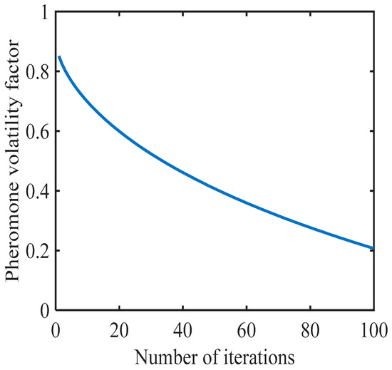
Figure 1.
Change curve of pheromone volatility factor.
Meanwhile, to prevent the algorithm from premature and stagnant searches, the pheromone concentration will be set within a certain range, defining the pheromone concentration in the range of . The equation is shown as (11).
where denotes the lower limit of pheromone concentration and denotes the upper limit.
3.3. Solving Deadlock Problems
When the environment is sophisticated, ants may be trapped in a deadlock state, and the algorithm will stall. Therefore, to avoid this situation, this paper uses backtracking to solve the deadlock phenomenon. Ren et al. [34] proposed that when ants fall into a deadlock, ants do not need to backtrack and directly abandon the current path for the next search. Qu et al. [35] allowed ants to backtrack one step and penalize the pheromone concentration at the side of deadlocks to prevent other ants from getting into the deadlock. Although the above strategies can guarantee the number of ants or decrease the computation and avoid the interference of inferior paths to other ants’ search, there will still be some path points that require more than one backoff to escape the deadlock phenomenon. As shown in Figure 2, the L1 path is caught in a U-shaped deadlock and requires multiple backtracking to unlock it, while the L2 path is caught in a deadlock only once and can find an optional path point after backtracking once. To deal with this difficulty, a new fallback strategy is adopted. When ants fall into a deadlock, the current path point is backed off until a valid path appears, and the path point that falls into the deadlock is set as an obstacle state to avoid subsequent ants falling into the deadlock repeatedly.
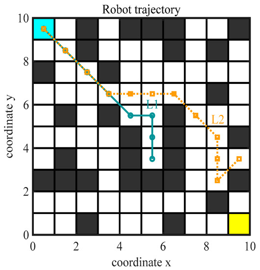
Figure 2.
Deadlock state diagram.
3.4. Improved Ant Colony Optimization Algorithm Flow
The pseudocode of the IACO in this paper is shown in Figure 3, and the specific steps are as follows.
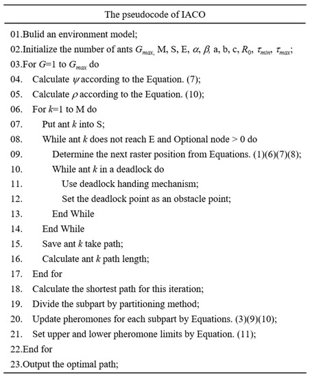
Figure 3.
The pseudocode of the improved ant colony optimization algorithm.
Step 1: Construct the environment model and initialize the parameters.
Step 2: Place the ants at the starting point and start searching.
Step 3: Path selection. Calculate the next selectable path point based on Equations (1) and (6)–(8) and judge whether the path point is in deadlock; if it is in deadlock, use the backoff mechanism to deal with it until the selectable path point appears, otherwise continue the search and update the taboo table (the taboo table is used to record the path points that have been tabooed to avoid the ants from repeatedly visiting the same paths or performing the same moves during the search).
Step 4: Judge whether ant completes a path search; if it does, save the path taken by ant , make , and go to Step 2 until all M ants complete a search. If not, go to Step 3 until ant completes a path search.
Step 5: Update the pheromone. When M ants complete one search, use the partition method to update the pheromone according to Equations (3), (4), (9), and (10), and the pheromone concentration is qualified by Equation (11).
Step 6: Check whether the termination condition is satisfied, and if so, output the optimal path length; otherwise, remove the taboo table, and then go to Step 2 and continue executing the loop until the termination condition is satisfied or reaches the maximum number of iterations.
4. Analysis of Simulation and Experimental Results
To demonstrate the effectiveness of the IACO in robot path planning, this paper will analyze the related performance of the algorithm through simulation experiments. The experimental environment is as follows: computer operating system is Win11 (64 bit), the processor is R7-5800H, memory is 16 GB, and the simulation platform is MATLAB R2021b.
4.1. Environment Modeling
The first step in solving the problem is to model the environment [36,37], and typical modeling methods include the grid method [38], the visual graph method [39], and the topological graph method [40]. The visual graph method is to connect all the obstacle vertices, and the connecting line cannot pass through the obstacle. That is to say, the straight line is visible, and at the same time, assign the corresponding weight to the edges in the graph to form graph G(A, E). Due to the simple structure of the grid method, which can effectively decrease the sophistication of the environment, this paper adopts the grid method for modeling [41,42].
The robot grid environment is shown in Figure 4a, where the black grid is the obstacle area and the white grid is the free area, and the whole environment corresponds to the matrix shown in Figure 4b [43,44]. Each grid within the robot grid environment is assigned a unique ordinal number based on its position from top to bottom and left to right, ranging from 1 to 100, with S and G indicating the starting and ending points, respectively [45,46]. However, in reality, many obstacles are irregular shapes, and we need to normalize them. When the area of an obstacle does not occupy the whole grid, we treat it as the entire grid, which will benefit the environment modeling [47]. The grid coordinates are represented by the (x, y) coordinates of the center point, and the conversion between the serial number and the corresponding coordinate is shown in Equation (12).
where is the edge length of the grid, usually recorded as one; and represent the total number of grids in the row and column directions, respectively; mod and ceil represent the modulo and floor functions, respectively.
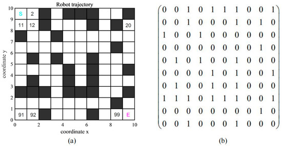
Figure 4.
Grid and the corresponding matrix diagram. (a) Grid environment map. (b) The matrix corresponding to the grid.
4.2. Parameter Optimization Selection
The solving ability of the ACO is influenced by several parameters, and the optimal set of combined parameters cannot be decided by the best theoretical method yet [48,49]. Therefore, to get the optimal solution, this paper uses a single control parameter value method for simulation experiments, and the combination of parameters is selected optimally by analyzing the test results for different parameter values [50].
4.2.1. Pheromone Heuristic Factor and Expectation Heuristic Factor
reflects the importance of the pheromone function to the ants when they move. If the value is too large, the probability of ants choosing the last path is large, and the search randomness will be weakened; if the value is too small, it will be similar to the greedy algorithm, making the search end with falling into local optimum [51]. reflects the importance of the heuristic function to the ants when they move. When is too large, it is difficult for the algorithm to obtain a better value, and when is too small, the ants will tend to choose a path based on the pheromone concentration [52].
The selection of parameters and is strongly interrelated, and the optimal performance of ACO requires both strong randomness and fast convergence. Therefore, the influence of the selection of the two on the performance of the ACO algorithm is complementary and closely related, and the algorithm has to find a suitable optimal value between them in order to obtain the optimal solution [53]. First, a range of values is set for and : and , and then a default value of and is selected as a starting point. In each experiment, only one parameter is changed, and the optimal path length, number of iterations, and number of ants lost are analyzed.
Figure 4a is used as the test environment for the combined experiment with the experimental parameters: , = 100, , , , and is taken as 0.1, 0.2, 0.3, ..., 2.0, respectively. From Figure 5, it can be seen that when is small, the ACO has blindness in the preliminary search; the number of ants lost is high, and many ants cannot reach the target point, while the IACO adopts the backtracking mechanism can validly solve the problem of ants caught in deadlock. When , IACO has faster convergence speed, and the number of iterations is only two. With the increase in , the global search capability of IACO and ACO gradually decreases and falls into local optimal solutions more easily. Overall, IACO outperforms ACO in terms of comprehensive performance.
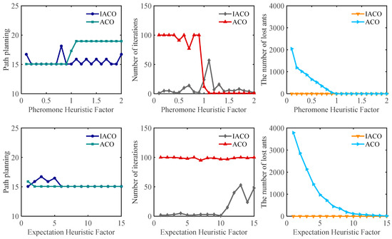
Figure 5.
The effect of and values on three different performance metrics.
Under the same environment, the following parameters are set: , = 100, , , . is taken as 1, 2, 3,..., 15, respectively. From Figure 5, it can be seen that when is small, IACO can easily be trapped in local optimization. When , IACO has a strong global search for optimal solutions and faster convergence speed, with an average shortest path length of 15.07 and an average number of iterations of 2.4. As increases, the convergence speed of IACO weakens, but still outperforms ACO. No matter how changes, there are zero ants lost in IACO.
4.2.2. Selection Factor
as a selection factor is usually set as a fixed constant, and different has a substantial influence on the randomness and convergence speed. When , the deterministic selection mode is used, and when , the random selection mode is used. In order to explore what value of the algorithm can obtain the best path length with, 10 simulations were conducted for each value of , and the path trajectory and path length of ant crawling were recorded for each simulation. Figure 6 shows the path trajectory of ant crawling when is taken as different values, Figure 7 shows the mean value of path length when 10 simulations were conducted for different values, and Figure 8 shows the box plot of the mean value of path length when 10 simulations were conducted for different values. The other parameters are taken as follows: , = 100, , , .
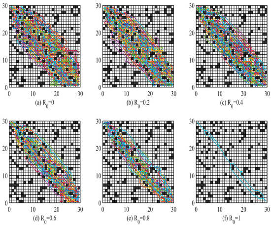
Figure 6.
Trajectories of ant crawling paths corresponding to different values.
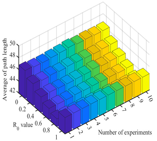
Figure 7.
Average value of path length for 10 simulations with different values.
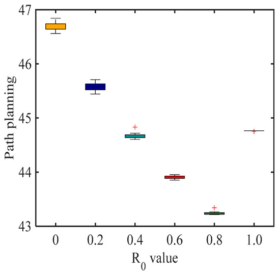
Figure 8.
Box plot of the mean value of path length for 10 simulations with different values.
Figure 6 shows that as the value of increases, the search range of ants decreases. As the value of increases, ants will tend to adopt the deterministic selection mode, which leads to the weakening of the randomness of ants in search, affects the search range of ants, and verifies the effectiveness of the value. Therefore, the range of IACO in the search can be regulated by the value of .
4.3. Analysis of Algorithm Practicality and Effectiveness
4.3.1. Improved Validity Verification of State Transfer Rules
To demonstrate the effectiveness of the state transfer rule on the improved algorithm, the improved state transfer rule will be incorporated on the basic ACO, and the path planning simulation experiments will be conducted with the basic ACO and IACO in a 30 × 30 grid environment (the simulation environment is illustrated in Figure 6). The experiment will be assessed using three performance indicators: the optimal path length, the number of convergences, and the number of inflection points. As ACO is a probabilistic optimization algorithm, to mitigate the impact of chance on the results, each experiment will be independently conducted 10 times. Figure 9 shows a comparison of the experimental results of the improved state transfer rules, where “IACOTest” means that only the improved transition rules are added to the ACO. The experimental parameters in the simulation are taken as: , = 100, , , , .
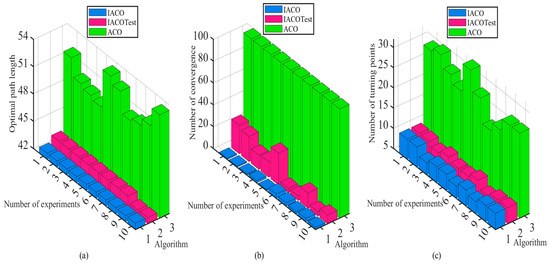
Figure 9.
Comparison of experimental results of improved state transfer rule. (a) Comparison of optimal path length. (b) Comparison of the number of convergences. (c) Comparison of the number of turning points.
From Figure 9a, it is shown that the average path lengths of IACOTest and IACO are 43.2148 and 42.674, respectively, and the average optimal path length of the traditional ACO is 51.1746. Compared to ACO, IACOTest improved by 15.55% and IACO improved by 16.61%, so it is obvious that the improved IACO in this paper has more advantages. From Figure 9b, it is shown that the average convergence times of IACOTest and IACO are 13.9 and 2, respectively, while the convergence times of the basic ACO are both 100 (which means that the algorithm has not converged). Compared with ACO, IACOTest improves by 86.1% and IACO improves by 98%, which shows that the introduction of the triangle inequality idea can make IACO greatly shorten the convergence time of the algorithm while ensuring the acquisition of the optimal solution. From Figure 9c, it is shown that the average number of inflection points of the IACOTest and IACO are 9.3 and 8.9, respectively, and the average number of inflection points of the traditional ACO is 26.6. Compared with ACO, the IACOTest improves 65.05% and IACO improves 66.54%. It is clear that IACO greatly improves the smoothness of the path and reduces the energy consumption when the robot moves while ensuring the optimal solution is obtained. In summary, improving the state transition rule by introducing the triangle inequality principle and pseudo-random state transition can not only reduce the path length and the convergence time when the robot moves, but also enhance the smoothness of the robot when moving.
4.3.2. Improved Validity Verification of Pheromone Update Rule
To demonstrate the effectiveness of the pheromone update rule for the improved algorithm, the improved pheromone update rule will be incorporated into the basic ACO, and path planning simulation experiments will be performed with the basic ACO and IACO in a 30 × 30 grid environment (the simulation environment is shown in Figure 6). The performance indicators analyzed in this experiment include the optimal path length, convergence times, and inflection points. The backtracking method will be used to solve deadlock problems for each algorithm. Since ACO is a probabilistic optimization algorithm, in order to avoid bias caused by algorithmic randomness, all experiments will be conducted independently 10 times. Figure 10 shows a comparison of the experimental results of the improved pheromone update rule, where “IACOTest” means that the improved pheromone update rule is added to the ACO. The experimental parameters in the simulation are taken as: , = 100, , , , .
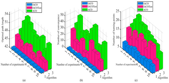
Figure 10.
Comparison of experimental results of improved pheromone update rule. (a) Comparison of optimal path length. (b) Comparison of the number of convergences. (c) Comparison of the number of turning points.
From Figure 10a, it is shown that the average path lengths of the IACOTest and IACO are 45.3844 and 42.674, respectively, while the average optimal path length for the traditional ACO is 50.9334. Compared to ACO, the IACOTest improved by 10.89% and IACO improved by 16.22%, so it is obvious that the improved IACO in this paper has more advantages. From Figure 10b, it is shown that the average convergence times of IACOTest and IACO are 20.1 and 2.4, respectively, while the convergence times of the basic ACO are 38.7. Compared with ACO, the IACOTest improves by 48.06% and IACO improves by 93.8%, which shows that taking different pheromone increments for the path segments can make IACO significantly shorten the convergence time of the algorithm while ensuring the optimal solution is obtained. From Figure 10c, it is shown that the average number of inflection points of IACOTest and IACO are 15.3 and 9, respectively, and the average number of inflection points of the traditional ACO is 19.5. Compared with ACO, the IACOTest improves 21.54% and IACO improves 53.85%. It is clear that IACO greatly improves the smoothness of the path and reduces the energy consumption when the robot moves while ensuring the optimal solution is obtained. In summary, the pheromone incremental update strategy based on the partitioning method for different path segments can distinguish the path segments, which is beneficial for the ants to search along the direction of the optimal path next time. The use of adaptive pheromone volatility factor can control the pheromone content, which enables the ants to obtain more effective paths and enhances the algorithm’s capability to explore space.
4.4. Simulation Verification of Different Environments
4.4.1. Case 1
To demonstrate the validity of the IACO, we performed simulation experiments on the MATLAB R2021b platform with ACO, Luo et al. [21], Liu et al. [22], Zheng et al. [25], and Gao and Wang [26] in the grid map of literature [21] and compared the simulation results of the six algorithms. Figure 11 shows the path planning results of each algorithm, and Figure 12 shows the convergence curve of each algorithm. To avoid the bias caused by algorithm chance, all experiments were conducted 10 times independently, and Table 1 shows the average results of 10 simulation experiments performed for each algorithm. The experimental parameters in the simulation are taken as: , = 100, , , , .
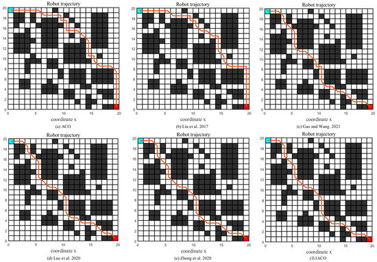
Figure 11.
Path planning diagram of six algorithms (ACO, improved ACO variant algorithms [21,22,25,26], IACO) in environment one.
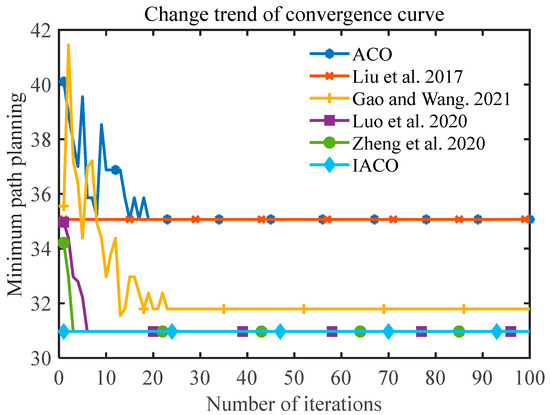
Figure 12.
The number of convergences of the six algorithms (ACO, improved ACO variant algorithms [21,22,25,26], IACO) in environment one.

Table 1.
Simulation data for the six algorithms in environment one.
From Figure 11 and Figure 12 and Table 1, we can see that ACO, Liu et al. [22] and Gao and Wang [26] find it more difficult to obtain the optimal value, and the ant survival rate and smoothness are low, which reduces the efficiency of the robot. The path length of Liu et al. [22] is 35.071, and it takes only 2.2 iterations on average to converge stably. It has a fast convergence speed, but it does not find the global optimum. The path length planned by Luo et al. [21] and Zheng et al. [25] is 30.968, which is 11.7% better compared to ACO. Although both converge to the global optimal solution and substantially improve the survival rate of ants, the IACO in this paper outperforms both of the above comparison algorithms in terms of performance, requiring only 1.8 iterations on average to converge to the optimal solution, and the survival rate of ants is 100%. This is because this paper adopts the idea of the backtracking method for unlocking, by backtracking the ants caught in the deadlock barrier until a valid path appears, which can guarantee the ant survival rate.
4.4.2. Case 2
To test the stability of the improved IACO, we carried out simulation experiments on the MATLAB R2021b platform with ACO, Li et al. [24], Gao and Wang [26], Miao et al. [27], and Wu et al. [42] in two grid maps of Miao et al. [27] and compared the simulation results of the six algorithms. Among them, the path planning results in the simple environment are shown in Figure 13, and the convergence curves are shown in Figure 14; the path planning results in the complex environment are shown in Figure 15, and the convergence curves are shown in Figure 16. To avoid bias caused by algorithm chance, all experiments were conducted 10 times independently, and Table 2 and Table 3 show the average results of 10 simulation experiments conducted for each algorithm in both environments.
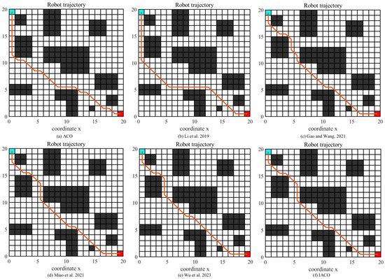
Figure 13.
Path planning diagram of six algorithms (ACO, improved ACO variant algorithms [24,26,27,42], IACO) in environment two.
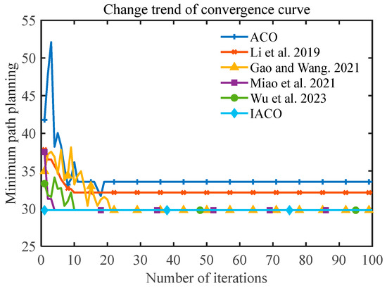
Figure 14.
The number of convergences of the six algorithms (ACO, improved ACO variant algorithms [24,26,27,42], IACO) in environment two.
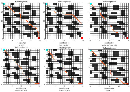
Figure 15.
Path planning diagram of six algorithms (ACO, improved ACO variant algorithms [24,26,27,42], IACO) in environment three.
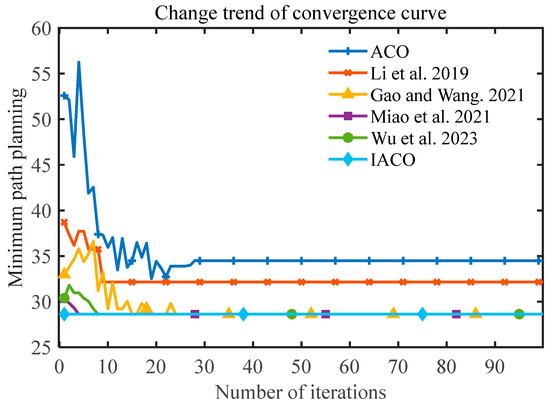
Figure 16.
The number of convergences of the six algorithms (ACO, improved ACO variant algorithms [24,26,27,42], IACO) in environment three.
Table 2.
Simulation data for the six algorithms in environment two.
Table 3.
Simulation data for the six algorithms in environment three.
From Figure 13 and Figure 14 and Table 2, it can be seen that the path length of ACO is 33.56 and the standard deviation reaches 3.4189, which indicates that the stability of ACO is not enough to obtain a quality solution. The Li et al. [24] study has the highest smoothness among the six algorithms, with only four turning points between the starting point and end point, which can obtain a smooth path and greatly reduce the energy consumption of the robot but cannot obtain a global optimal solution. Gao and Wang [26], Miao et al. [27], and Wu et al. [42] can obtain the global optimum after certain iterations, which is 11.22% better than ACO, but IACO is better than the above comparison algorithms in terms of performance indexes, and IACO only needs 1.8 iterations on average to converge to the global optimum solution with a standard deviation of 0.6. Thus, it can be clearly seen that IACO still has a high smoothness while ensuring faster convergence, which can obtain better optimal solutions and achieve an overall optimal path planning performance.
From Figure 15 and Figure 16 and Table 3, it is shown that when the proportion of obstacles in the environment increases, the IACO can still converge to the optimal path quickly with a length of 28.624, which is an 11% improvement in path length compared with the Li et al. [24]. In terms of smoothness of path planning, the IACO in this paper only needs seven corner turns to reach the end point, which is a 59% improvement in smoothness compared to ACO and greatly reduces the energy consumption of the robot. In terms of the number of convergences, IACO only needs 1 iteration to converge to the optimal solution at the earliest and only 1.7 iterations on average, which is an 87.5% improvement compared with the Wu et al. [42]. Therefore, IACO is able to achieve global optimal performance in an environment with a large proportion of obstacles while ensuring a certain diversity of algorithms, especially in terms of the smoothness and convergence times.
4.4.3. Case 3
To verify the effectiveness of the IACO in a high-dimensional environment, simulation experiments are conducted in this section in a 30-dimensional grid environment by Zhang et al. [28], and the simulation results are compared with those of ACO, Zhang et al. [28], Wu et al. [42], A* algorithm, and Dijkstra algorithm. The path planning results are shown in Figure 17. To avoid errors caused by algorithmic chance, all experiments were performed 10 times, and the results were averaged as shown in Table 4. represents the optimal path length, represents the maximum path length, represents the average path length, represents the standard deviation of the path length, indicates the number of iterations to obtain the global optimum for the first time, indicating the convergence speed of the algorithm, and represents the success rate of obtaining the global optimum 10 times, showing the stability of the algorithm. Turns times indicates the number of turning points.
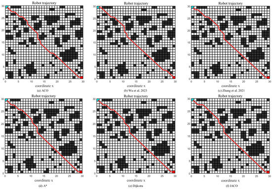
Figure 17.
The number of convergences of the six algorithms (ACO, improved ACO variant algorithms [28,41], A*, Dijkstra, IACO) in environment four.
Table 4.
Simulation data for the six algorithms in environment four.
Based on the data in Figure 17 and Table 4, it can be concluded that the IACO still converges to the optimal solution quickly when the environment is expanded to 30 dimensions, and the optimal solution of 42.7696 can be reached in only one iteration on average. Compared with the traditional ACO, the improved algorithm improves by 1.4% in terms of path length. In terms of smoothness, the IACO only needs seven corner turns to reach the endpoint, which enhances the smoothness by 47.2% compared with the ACO. Taken together, the IACO proposed in this paper can enable the robot to obtain a better comprehensive performance path.
To summarize, under four map environments with different obstacle ratios, the proposed algorithm has substantially improved compared with the basic ACO and other improved algorithms, effectively reducing the path length and the number of redundant corners and also improving the operation efficiency of the algorithm, which verifies the effectiveness and stability of the proposed algorithm.
5. Conclusions
In this paper, an improved ant colony optimization algorithm based on the triangle inequality idea, a pseudo-random state transfer strategy, the partitioned pheromone update model, and the backtracking mechanism are proposed to enhance the efficiency when the robot is running. The triangle inequality idea can make the ants more inclined to choose the path that is biased toward the goal point and accelerate the convergence of the algorithm. The introduction of a pseudo-random state transfer strategy can improve the efficiency and quality of the search for optimal solutions. The pheromone increment strategy based on the partition method is applied to update each path segment separately, which shortens the convergence time of the algorithm while setting the pheromone in a certain interval range to avoid premature and stagnation phenomena of the algorithm during the search. The idea of backtracking is used to unlock the ants caught in a deadlock, which enhances the search capability of the ants for solution spacing. The proposed algorithm is applied to mobile robot path planning and compared with several improved algorithms. Simulation results demonstrate that the improved ant colony optimization algorithm outperforms its comparison algorithm in terms of performance index and adaptability to different environments.
Author Contributions
S.W.: formal analysis, investigation, and writing. Q.L. and W.W.: methodology, supervision, and writing. All authors have read and agreed to the published version of the manuscript.
Funding
The Key Project of Science and Technology Innovation 2030 supported by the Ministry of Science and Technology of China (No. 2018AAA0101301), the Key Projects of Artificial Intelligence of High School in Guangdong Province (No. 2019KZDZX1011), Dongguan Social Development Science and Technology Project (No. 20211800904722) and Dongguan Science and Technology Special Commissioner Project (No. 20221800500052).
Data Availability Statement
The all data presented in the article does not require copyright. They are freely available from the authors.
Acknowledgments
The authors thank the reviewers for their valuable comments on the article, which helped to embellish the article.
Conflicts of Interest
The authors state that there is no conflict of interest between them.
References
- Sudhakara, P.; Ganapathy, V.; Priyadharshini, B.; Sundaran, K. Obstacle avoidance and navigation planning of a wheeled mobile robot using amended artificial potential field method. Procedia Comput. Sci. 2018, 133, 998–1004. [Google Scholar] [CrossRef]
- Han, J.; Seo, Y. Mobile robot path planning with surrounding point set and path improvement. Appl. Soft Comput. 2017, 57, 35–47. [Google Scholar] [CrossRef]
- Wang, L.; Wang, H.; Yang, X.; Gao, Y.; Cui, X.; Wang, B. Research on smooth path planning method based on improved ant colony algorithm optimized by Floyd algorithm. Front. Neurorobot. 2022, 16, 955179. [Google Scholar] [CrossRef] [PubMed]
- Dijkstra, E. A note on two problems in connexion with graphs. Numer. Math. 1959, 1, 269–271. [Google Scholar] [CrossRef]
- Alshammrei, S.; Boubaker, S.; Kolsi, S. Improved Dijkstra Algorithm for Mobile Robot Path Planning and Obstacle Avoidance. Comput. Mater. Contin. 2022, 72, 5939–5954. [Google Scholar] [CrossRef]
- Zhong, X.Y.; Tian, J.; Hu, H.S.; Peng, X.F. Hybrid Path Planning Based on Safe A* Algorithm and Adaptive Window Approach for Mobile Robot in Large-Scale Dynamic Environment. J. Intell. Robot. Syst. 2020, 99, 65–77. [Google Scholar] [CrossRef]
- Liu, A.; Jiang, J. Solving path planning problem based on logistic beetle algorithm search-pigeon-inspired optimisation algorithm. Electron. Lett. 2022, 56, 1105–1107. [Google Scholar] [CrossRef]
- Zhang, F.; Bai, W.; Qiao, Y.; Zhou, P. UAV indoor path planning based on improved D* algorithm. CAAI Trans. Intell. Syst. 2019, 14, 662–669. [Google Scholar]
- Xie, K.; Qiang, J.; Yang, H. Research and Optimization of D-Start Lite Algorithm in Track Planning. IEEE Access 2020, 8, 161920–161928. [Google Scholar] [CrossRef]
- Jiang, X.; Deng, Y. UAV Track Planning of Electric Tower Pole Inspection Based on Improved Artificial Potential Field Method. J. Appl. Sci. Eng. 2021, 24, 123–132. [Google Scholar]
- Xu, T.; Zhou, H.; Tan, S.; Li, Z.; Ju, X.; Peng, Y. Mechanical arm obstacle avoidance path planning based on improved artificial potential field method. Ind. Robot 2022, 49, 271–279. [Google Scholar] [CrossRef]
- Song, B.; Wang, Z.; Sheng, L. A new genetic algorithm approach to smooth path planning for mobile robots. Assem. Autom. 2016, 36, 138–145. [Google Scholar] [CrossRef]
- Chen, X.; Gao, P. Path planning and control of soccer robot based on genetic algorithm. J. Ambient Intell. Humaniz. Comput. 2020, 11, 6177–6186. [Google Scholar] [CrossRef]
- Tan, Y.; Jie, O.; Zhang, Z.; Lao, Y.; Wen, P. Path planning for spot welding robots based on improved ant colony algorithm. Robotica 2023, 41, 926–938. [Google Scholar] [CrossRef]
- Li, X.; Wang, L. Application of improved ant colony optimization in mobile robot trajectory planning. Math. Biosci. Eng. 2020, 17, 6756–6774. [Google Scholar] [CrossRef]
- Qiang, N.; Gao, J.; Kang, F. Multi-Robots Global Path Planning Based on PSO Algorithm and Cubic Spline. J. Syst. Simul. 2017, 29, 1397–1404. [Google Scholar]
- Xu, L.; Cao, M.; Song, B. A new approach to smooth path planning of mobile robot based on quartic Bezier transition curve and improved PSO algorithm. Neurocomputing 2022, 473, 98–106. [Google Scholar] [CrossRef]
- Zhang, W.; Zhang, S.; Wu, F.; Wang, Y. Path Planning of UAV Based on Improved Adaptive Grey Wolf Optimization Algorithm. IEEE Access 2021, 9, 89400–89411. [Google Scholar] [CrossRef]
- Liu, J.; Wei, X.; Huang, H. An Improved Grey Wolf Optimization Algorithm and its Application in Path Planning. IEEE Access 2021, 9, 121944–121956. [Google Scholar] [CrossRef]
- Hao, K.; Zhang, H.; Li, Z.; Liu, Y. Path Planning of Mobile Robot Based on Improved Obstacle Avoidance Strategy and Double Optimization Ant Colony Algorithm. Trans. Chin. Soc. Agric. Mach. 2022, 53, 303–312, 422. [Google Scholar]
- Luo, Q.; Wang, H.; Zheng, Y.; He, J. Research on path planning of mobile robot based on improved ant colony algorithm. Neural Comput. Appl. 2020, 32, 1555–1566. [Google Scholar] [CrossRef]
- Liu, J.; Yang, J.; Liu, H.; Tian, X.; Gao, M. An improved ant colony algorithm for robot path planning. Soft Comput. 2017, 21, 5829–5839. [Google Scholar] [CrossRef]
- Akka, K.; Khaber, F. Mobile robot path planning using an improved ant colony optimization. Int. J. Adv. Robot. Syst. 2018, 15. [Google Scholar] [CrossRef]
- Li, L.; Li, H.; Shan, N. Path Planning Based on Improved Ant Colony Algorithm with Multiple Inspired Factor. Comput. Eng. Appl. 2019, 55, 219–225, 250. [Google Scholar]
- Zheng, Y.; Luo, Q.; Wang, H.; Wang, C.; Chen, X. Path planning of mobile robot based on adaptive ant colony algorithm. J. Intell. Fuzzy Syst. 2020, 39, 5329–5338. [Google Scholar] [CrossRef]
- Gao, M.; Wang, H. Path planning for mobile robots based on improved ant colony algorithm. Transducer Microsyst. Technol. 2022, 40, 142–144, 148. [Google Scholar]
- Miao, C.; Chen, G.; Yan, C.; Wu, Y. Path planning optimization of indoor mobile robot based on adaptive ant colony algorithm. Comput. Ind. Eng. 2021, 156, 107230. [Google Scholar] [CrossRef]
- Zhang, S.; Pu, J.; Si, Y. An Adaptive Improved Ant Colony System Based on Population Information Entropy for Path Planning of Mobile Robot. IEEE Access 2021, 9, 24933–24945. [Google Scholar] [CrossRef]
- Pu, X.; Song, X. Improvement of ant colony algorithm in group teaching and its application in robot path planning. CAAI Trans. Intell. Syst. 2022, 17, 764–771. [Google Scholar]
- Tang, X.; Xin, S. Improved Ant Colony Algorithm for Mobile Robot Path Planning. Comput. Eng. Appl. 2022, 58, 287–295. [Google Scholar]
- Wang, L. Path planning for unmanned wheeled robot based on improved ant colony optimization. Meas. Control 2020, 53, 1014–1021. [Google Scholar] [CrossRef]
- Li, X.; Yu, D. Study on an Optimal Path Planning for a Robot Based on an Improved ANT Colony Algorithm. Autom. Control Comput. Sci. 2019, 53, 236–243. [Google Scholar]
- Tian, H. Research on robot optimal path planning method based on improved ant colony algorithm. Int. J. Comput. Sci. Math. 2021, 13, 80–92. [Google Scholar] [CrossRef]
- Ren, H.; Hu, H.; Shi, T. Mobile robot dynamic path planning based on improved ant colony algorithm. Mod. Electron. Tech. 2021, 44, 182–186. [Google Scholar]
- Qu, H.; Huang, L.; Ke, X. Research of Improved Ant Colony Based Robot Path Planning Under Dynamic Environment. J. Univ. Electron. Sci. Technol. China 2015, 44, 260–265. [Google Scholar]
- Mac, T.; Copot, C.; Tran, D.; Keyser, R. Heuristic approaches in robot path planning: A survey. Robot. Auton. Syst. 2016, 86, 13–28. [Google Scholar]
- Ajeil, F.; Ibraheem, I.; Azar, A.; Humaidi, A. Grid-Based Mobile Robot Path Planning Using Aging-Based Ant Colony Optimization Algorithm in Static and Dynamic Environments. Sensors 2020, 20, 1880. [Google Scholar]
- Yang, L.; Fu, L.; Li, P.; Mao, J.; Guo, N.; Du, L. LF-ACO: An effective formation path planning for multi-mobile robot. Math. Biosci. Eng. 2022, 19, 225–252. [Google Scholar] [CrossRef]
- Chen, C.; Tang, J.; Jin, Z.; Yang, Y.; Qian, L. A Path Planning Algorithm for Seeing Eye Robots Based on V-Graph. Mech. Sci. Technol. Aerosp. Eng. 2014, 33, 490–495. [Google Scholar]
- Das, P.; Jena, P. Multi-robot path planning using improved particle swarm optimization algorithm through novel evolutionary operators. Appl. Soft Comput. 2020, 92, 106312. [Google Scholar] [CrossRef]
- Zhang, T.; Wu, B.; Zhou, F. Research on Improved Ant Colony Algorithm for Robot Global Path Planning. Comput. Eng. Appl. 2022, 58, 282–291. [Google Scholar]
- Wu, S.; Wei, W.; Zhang, Y.; Ye, Z. Path Planning of Mobile Robot Based on Improved Ant Colony Algorithm. J. Dongguan Univ. Technol. 2023, 30, 24–34. [Google Scholar]
- Dai, X.; Long, S.; Zhang, Z.; Gong, D. Mobile Robot Path Planning Based on Ant Colony Algorithm With A* Heuristic Method. Front. Neurorobot. 2019, 13, 15. [Google Scholar] [CrossRef] [PubMed]
- Zhu, S.; Zhu, W.; Zhang, X.; Cao, T. Path planning of lunar robot based on dynamic adaptive ant colony algorithm and obstacle avoidance. Int. J. Adv. Robot. Syst. 2020, 17, 4149–4171. [Google Scholar] [CrossRef]
- Liu, N.; Wang, H. Path planning of mobile robot based on the improved grey wolf optimization algorithm. Electr. Meas. Instrum. 2020, 57, 76–83, 98. [Google Scholar]
- Ma, F.; Qu, Z. Research on path planning of mobile robot based on heterogeneous dual population and global vision ant colony algorithm. Appl. Res. Comput. 2022, 39, 1705–1709. [Google Scholar]
- Zhang, H.; He, L.; Yuan, L.; Ran, T. Mobile robot path planning using improved double-layer ant colony algorithm. Control Decis. 2022, 37, 303–313. [Google Scholar]
- Zhang, H.; Lin, W.; Chen, A. Path Planning for the Mobile Robot: A Review. Symmetry 2018, 10, 450. [Google Scholar] [CrossRef]
- Erin, B.; Abiyev, R.; Ibrahim, D. Teaching robot navigation in the presence of obstacles using a computer simulation program. Procedia Soc. Behav. Sci. 2010, 2, 565–571. [Google Scholar] [CrossRef]
- Zhang, C.; Hu, C.; Feng, J.; Liu, Z.; Zhou, Y.; Zhang, Z. A Self-Heuristic Ant-based Method for Path Planning of Unmanned Aerial Vehicle in Complex 3-D Space with Dense U-type Obstacles. IEEE Access 2019, 7, 150775–150791. [Google Scholar] [CrossRef]
- He, Y.; Fan, X. Application of Improved Ant Colony Optimization in Robot Path Planning. Comput. Eng. Appl. 2021, 57, 276–282. [Google Scholar]
- Yuan, F.; Zhu, J. Optimal path planning of mobile robot based on improved ant colony algorithm. Mod. Manuf. Eng. 2021, 7, 38–47, 65. [Google Scholar]
- Wang, L.; Kan, J.; Guo, J.; Wang, C. 3D Path Planning for the Ground Robot with Improved Ant Colony Optimization. Sensors 2019, 19, 815. [Google Scholar] [CrossRef] [PubMed]
Disclaimer/Publisher’s Note: The statements, opinions and data contained in all publications are solely those of the individual author(s) and contributor(s) and not of MDPI and/or the editor(s). MDPI and/or the editor(s) disclaim responsibility for any injury to people or property resulting from any ideas, methods, instructions or products referred to in the content. |
© 2023 by the authors. Licensee MDPI, Basel, Switzerland. This article is an open access article distributed under the terms and conditions of the Creative Commons Attribution (CC BY) license (https://creativecommons.org/licenses/by/4.0/).