Article

Design of Finite Difference Method and Neural Network Approach for Casson Nanofluid Flow: A Computational Study

by
Muhammad Shoaib Arif
1,2,*,
Kamaleldin Abodayeh
1,* and
Yasir Nawaz
2
1
Department of Mathematics and Sciences, College of Humanities and Sciences, Prince Sultan University, Riyadh 11586, Saudi Arabia
2
Department of Mathematics, Air University, PAF Complex E-9, Islamabad 44000, Pakistan
*
Authors to whom correspondence should be addressed.
Axioms 2023, 12(6), 527; https://doi.org/10.3390/axioms12060527
Submission received: 15 April 2023 / Revised: 10 May 2023 / Accepted: 16 May 2023 / Published: 27 May 2023

Abstract

:
To boost productivity, commercial strategies, and social advancement, neural network techniques are gaining popularity among engineering and technical research groups. This work proposes a numerical scheme to solve linear and non-linear ordinary differential equations (ODEs). The scheme’s primary benefit included its third-order accuracy in two stages, whereas most examples in the literature do not provide third-order accuracy in two stages. The scheme was explicit and correct to the third order. The stability region and consistency analysis of the scheme for linear ODE are provided in this paper. Moreover, a mathematical model of heat and mass transfer for the non-Newtonian Casson nanofluid flow is given under the effects of the induced magnetic field, which was explored quantitatively using the method of Levenberg–Marquardt back propagation artificial neural networks. The governing equations were reduced to ODEs using suitable similarity transformations and later solved by the proposed scheme with a third-order accuracy. Additionally, a neural network approach for input and output/predicted values is given. In addition, inputs for velocity, temperature, and concentration profiles were mapped to the outputs using a neural network. The results are displayed in different types of graphs. Absolute error, regression studies, mean square error, and error histogram analyses are presented to validate the suggested neural networks’ performance. The neural network technique is currently used on three of these four targets. Two hundred points were utilized, with 140 samples used for training, 30 samples used for validation, and 30 samples used for testing. These findings demonstrate the efficacy of artificial neural networks in forecasting and optimizing complex systems.

1. Introduction

The study of heat exchange is well known for its extensive applications in furnaces, nuclear reactors, thermal energy storage systems, and temperature exchangers. To experience a better heat exchange rate, a heat transfer coefficient is named the Nusselt number, which motivates research in this field. In the Casson fluid flow in the direction of a stretched sheet, the heat transfer feature of the Casson fluid model [1] is developed in [2]. The focus of [2] was to calculate heat exchange characteristics with viscous dissipation in addition to the equation describing heat movement. The results revealed that velocity ratio parameters and Prandtl and Eckert numbers controlled Casson fluid flow. To generate analytical solutions, however, it was necessary to consider the full geographical domain, which is why the Homotopy analysis method (HAM) was developed. Sawati [3] studied the effect of non-linear extension on heat transfer in the Casson fluid flow.
Suitable transformation procedures were used to convert momentum and energy equations into reduced ones. Additionally, the numeric of the solutions were deduced using the shooting approach following the high temperature and reduced field velocity for the Casson parameter. Using mixed convection, Sawati et al. [4] analyzed the heat transfer in Casson fluid over a symmetric wedge. This study was also characterized by the use of a shooting methodology for graphic outcomes and examined how an increase in the Falkner–Skan exponent caused an increase in the velocity component with a fall in temperature. It also revealed that an increase in the Prandtl number resulted in a temperature fall. In the presence of suction or blowing [5], the boundary layer flow of a Casson fluid coupled with heat transfer along an infinitely extending surface was studied. Temperature field equations contained a thermal radiation factor, and transformation principles were used to convert momentum and energy transmission. The results revealed the opposite nature of velocity and temperature towards Casson fluid; therefore, efficient thermal diffusivity was obtained due to the rise in temperature due to thermal radiations.
Mahdy [6] investigated how to suction or blow and how the Soret and Dufour effects affected the flow and heat transfer of a non-Newtonian fluid outside of a stretching permeable cylinder using numerical solutions. Non-Newtonian fluid behavior was modeled using the Casson fluid equations.
Heat and mass transfer were used to investigate the instability of the flow of a Casson fluid approaching its stagnation point across a stretching/shrinking sheet subjected to thermal radiation [7]. The linear Rosseland approximation for heat radiation was also taken into account, as was the impact of a binary chemical reaction with Arrhenius activation energy. Numerical solutions to non-linear PDEs were found using a novel technique known as bivariate spectral collocation quasi-linearization. The resulting PDEs were static over all time and space, but the visual discussion of physical characteristics such as velocity, temperature, and concentration was presented. Using gyrotactic microorganisms, researchers studied the impact of thermophoresis and Brownian motion on a radiative Casson fluid in a two-dimensional magnetohydrodynamics (MHD) model [8]. Prioritized by [8] was the employment of Runge–Kutta and Newton’s methods, which were implemented numerically to produce graphical outputs. The distributions of velocities, temperatures, concentrations, and densities of movable organisms were analyzed in two cases of suction flow to determine the impact of the relevant parameters.
Comparing this study’s results to the literature revealed that the temperature and concentration field was directly proportional to the thermophoresis parameter values. This study also found that gyrotactic bacteria could boost mass and heat transmission. Reddy et al. [9] investigated how the development of conjugate heat transfer (CHT) altered the standard definition of heat function. Casson fluid was filled in a thin vertical cylinder whose inner walls were at a constant temperature. Linked, non-linear governing equations were solved using an implicit methodology and displayed graphically, whereas Casson fluid parameters were prolonged. The superiority of Casson fluid over Newtonian fluid could be illustrated by the fact that increasing the values of all controlling parameters typically resulted in less heat being lost from the hot outer wall [10]. This allowed us to study the effect of nanoparticles in suspension on an inclined plate when subjected to a Casson fluid flow regime.
The effects of frictional heating, heat generation, and thermal radiation were computed using a diffusion equation, and T i O 2 water and C u O water were used as nanofluids. A new analytical method was developed to address the difficulty of solving partial differential equations (PDEs). Mass, momentum, heat transit rates, and their dependence on significant flow factors were also investigated. Limited chemical reactions and heat radiation were found to be responsible for the increased thermal and mass transfer rate. The pulsating flow of a non-Newtonian micropolar-Casson fluid under the effect of the Lorentz force, according to Darcy’s law, was studied by Ali et al. [11]. A drop in wall shear stress was observed with increasing porosity, indicating an inverse relationship between the two. At the same time, the Hartman number had a major impact on the flow separation zone. All axial positions exhibited parabolic velocity, with a notable rise in the speed close to the constriction’s throat.
Casson fluid flow is considered in [12] across an extending, slanted cylinder surface. There is a mathematical description of the flow field. We resorted to a firing system to obtain precise numerical information about the cylinder’s surface’s heat transfer coefficient. Alizadeh et al. [13] took into account the after-effects of Soret and Dufour’s work. Sherwood, Nusselt, and Bejan numbers were derived from backing up the numerical solution of the flow equation. The Nusselt number was shown to drop more than Sherwood’s number in the results. Non-Newtonian features of the fluid were shown to have a significant bearing on flow temperature and mass transfer irreversibility.
The Casson time-independent nanofluid based on heat movements and entropy calculations was examined by Jamshed et al. [14]. Casson nanofluid flow convection was subjected to a slipper surface to calculate the slip state, flow characteristics, and thermal transport. PDEs were drawn and then converted into ODEs, and their self-solutions were driven using the numerical Keller box technique. An increase in the Reynold number resulted in the surged entropy of the system, whereas in the Casson phenomenon, thermal conductivity increased. In [15], the simultaneous heat and mass transfer fluid flow toward inclined flat and cylindrical surfaces was studied. It was generally agreed that Casson fluid is a model of a non-Newtonian fluid. The stagnation zone heat and mass transport analysis of a hybrid nanomaterial Casson fluid flowing over a vertical Riga sheet was conducted. This formulation incorporated Lorentz forces into the system when simulating flows through a medium containing a Riga sheet [16]. The present study [17] examined the time-independent behavior of nanofluid flow with non-Newtonian characteristics in a two-dimensional setting around a circular stretching cylinder. The utilization of magnetic effects in the direction perpendicular to the flow has been studied in relation to the Casson–Sutterby nanofluid. The authors in reference [18] proposed a numerical scheme to solve a mathematical model that accounted for the boundary layer flow over a sheet with electrical and magnetic effects. The methodology comprised two distinct stages: the predictor stage and the corrector stage. The predictor stage employed the dependent variable’s first- and second-order derivative in the differential equation provided.
Today, artificial intelligence profoundly relies on artificial neural networks (ANNs). ANNs own the property of refabricating and are involved in forming models based on non-linear phenomena; therefore, they possess a wide range of fields that engage young researchers. System identification, sequence recognition, process control, sensor data analysis, natural resource management, quantum chemistry, data mining, pattern recognition, medical diagnosis, finance, visualization, machine translation, e-mail spam filtering, and social network filtering are just some examples of the many fields that make extensive use of ANNs. ANNs are multidimensional and based on the input that flows via the network during learning; ANNs are well-known for their efficient and feasible backpropagation of stochastic numerical techniques. Backpropagation can be defined as a controlled learning method that is characterized by a gradient descent approach to decrease the gradient of the error curve, hence lessening the chance of an error being produced.
The backpropagation technique was originally developed by Paul Werbos in 1974 and was rediscovered by Rumelhart and Parker. For example, many feed-forward multilayer neural networks employ the backpropagation algorithm for learning. The Levenberg–Marquardt (LM) backpropagation is a novel technique in the field of ANNs that provides numerical solutions to numerous problems involving fluid flow. Some writers have used a Levenberg–Marquardt back-propagating artificial neural network (ANN) in conjunction with Newtonian and non-Newtonian fluid systems to achieve well-defined convergent stability (LBM-BN). Ly et al. [19] performed a metaheuristic analysis of the specifications and structure of LBM-BN, which could rapidly and reliably predict the shear capacity of foamed concrete. Using the LBM-BN technique, Zhao et al. [20] assessed the defect of reinforced concrete beams. Nguyen et al. [21] investigated ANN-based LM to boost robot placement accuracy. Ali et al. [22] used an ANN and an LM-based training technique to predict the volume of water that would flow over a weir with a steep crest. Ye and Kim [23] used the LBM-BN method to assess a building’s energy consumption in China. Bharati et al. [24] developed a novel systematic mechanism using a neuro-fuzzy system framework and self-organizing maps to analyze superconductor prediction.
ANNs are gaining a profound interest in literary society to solve real-life problems. These have a wide range of applications and possess versatile domains to encounter fluid dynamic issues and solve them numerically and analytically. ANNs, compared to old techniques, are more efficient at forming deterministic computing models and can produce more reliable and accurate results for stochastic numerical computational analysis. Today, the major focus of young researchers relies on ANNs due to their validation and precision; therefore, there is a plethora of research in the literature on the subject, including but not limited to entropy-generated systems [25], porous fins [26], COVID-19 [27], hydromagnetic Williamson fluid flow [28], carbon nanotubes [29], the Emden–Fowler equation [30], second-order singular functional differential models [31], Darcy–Forchheimer models [32], dissipative fluid flow systems [33], mosquito dispersal models [34] and many others [35,36,37,38]. A deep learning technique for estimating the boiling heat transfer coefficient of nanoporous coated surfaces was developed by the authors of [39]. Over the years, nanoporous-coated surfaces have been widely employed to boost boiling efficiency.
Numerical schemes can be considered tools for solving problems in applied sciences and engineering. There exist various numerical methods in the literature that can be used to solve a variety of problems. There may exist more than one numerical scheme to solve particular differential equations. However, different schemes have different characteristics that may depend on the order of accuracy, stability, and consumption time. This attempt was based on the numerical scheme that provided third-order accuracy in two stages. It is an explicit scheme that requires no linearization when solving non-linear differential equations. The method can be applied to solve second and third-order boundary value problems. For handling these boundary value problems, some initial conditions are assumed, and these assumed missing initial conditions could be found by applying the shooting method.
The proposed technique took too long to find extra derivatives of dependent variables. However, it provides third-order accuracy in two stages and is also an explicit scheme. Most explicit schemes do not have this kind of feature in the literature. They provide this accuracy in two stages. To ensure that the fluid flowing over the sheet is an incompressible, two-dimensional, stable, laminar Casson fluid under the effects of the induced magnetic field. The second aim of this paper was to use the power of artificial back-propagated neural networks with a Levenberg–Marquardt backpropagation algorithm to augment the computing power and level of accuracy in the solver.
Artificial neural network techniques are becoming increasingly popular among engineering and technical research organizations to increase productivity, business tactics, and social progress. Instead of implementing a wide variety of linear and non-linear mathematical frameworks, artificial intelligence-based stochastic solution techniques are being used. The mathematical representations of such fluid flow issues can be described by a system of very non-linear ordinary differential equations (ODEs). These methods for solving them were created using a modern computer paradigm. So far, this method has not been applied to the suggested issue. Employing a cutting-edge stochastic solution strategy founded on the artificial intelligence algorithm, this unique method can address the issue of supervised learning by employing intelligent computing techniques for the dynamics of fluid flow models.
The most important points of the situation are discussed below:
  • To resolve first-order linear and non-linear ordinary differential equations (ODEs), the third-order numerical technique has been put forward as a potential solution in two stages.
  • The construction of a computational numerical scheme is considered to solve the proposed mathematical model of the heat and mass transfer of non-Newtonian Casson nanofluid flow.
  • The proposed numerical scheme is highly accurate and attains the predicted order of convergence shown through various examples.
  • To verify the scheme’s efficacy, a couple of non-linear examples and a few real-life problems can be solved.
  • The mathematical model of heat and mass transfer of non-Newtonian Casson nanofluid flow is given under the induced magnetic field’s effects. Its numerical performance is provided through stochastic processes based on Levenberg–Marquardt backpropagation artificial neural networks.
  • Accuracy evaluations, histograms, and regression analysis for the fluid flow model are provided in sufficient graphical and numerical detail to validate and verify the Levenberg–Marquardt backpropagation technique.

2. Numerical Scheme

The proposed numerical scheme is constructed on two grid points that consist of two stages. Both stages of the scheme are explicit. However, the second-order derivative of the dependent variables is necessary for the first step. Therefore, one extra derivative in the scheme solves the first-order differential equation. However, this gives an advantage over the order of accuracy of the scheme. In this way, the scheme becomes third-order accurate in two stages; as mentioned earlier, it is an explicit scheme. To propose a scheme, the first-order differential equation can be considered as:
y = λ y
which is subject to the initial conditions:
y 0 = α 1
The first stage of the scheme for discretizing Equation (1) can be expressed as:
y i + 1 = y i + h y i + c h 2 y i
A first stage is an extended form of the Taylor scheme with the involvement of some constants. The second stage of the scheme can be given as:
y i + 1 = 1 4 3 y i + y i + 1 + h a y i + 1 + b y i
The second stage of the scheme finds the solution at the i t h grid point using the information on the “ i 1 t h ” grid point. At the same time, the first stage finds the solution on assumed grid points. The first-stage solution can be utilized in the second-stage solution. The first stage of the scheme is called the predictor stage, and the second stage can be called the corrector stage of the scheme. The second stage involves two unknown values that can be found by applying the Taylor series in Equation (4). However, before applying the Taylor series first stage is utilized in Equation (4) as:
y i + 1 = 1 4 4 y i + h y i + c h 2 y i + h a y i + a h y i + a c h 2 y i + b y i
before applying Taylor series expansion for y i + 1 as:
y i + 1 = y i + h y i + h 3 2 y i + h 3 6 y i + O h 4
Substituting Equation (5) into Equation (6) yields:
y i + h y i + h 3 2 y i + h 3 6 y i = 1 4 4 y i + h y i + c h 2 y i + h a y i + a h y i + a c h 2 y i + b y i
Comparing the coefficients of h y i , h 2 y i and h 3 y i on both sides of Equation (7) yields:
3 4 = a + b
1 2 = c 4 + a + b
1 6 = a 2 + b c
Solving Equations (8)–(10) yields:
a = 11 18 , b = 5 36   and   c = 1
Therefore, the first and second stages of the scheme can be expressed as follows:
y i + 1 = y i + h y i h 2 y i
y i + 1 = 1 4 3 y i + y i + 1 + h 11 18 y i + 1 + 5 36 y i

3. Stability Analysis

To find the stability conditions for Equation (1), the first stage of the scheme gives:
y i + 1 = y i + λ h y i λ 2 h 2 y i + 1
where y i = λ y i and y i = λ 2 y i .
Equation (14) can be expressed as:
y i + 1 = y i 1 + λ h λ 2 h 2 = 1 + z z 2 y i
where z = h λ .
The second stage of the suggested strategy to Equation (1) can be applied as follows:
y i + 1 = 1 4 3 y i + y i + 1 + h 11 18 λ y i + 5 36 λ y i
By utilizing Equation (15) in Equation (16), it provides:
y i + 1 = 1 4 3 y i + y i + 1 + h 11 18 λ 1 + z z 2 y i + 5 36 λ y i = 1 4 3 y i + 1 + z z 2 y i + 11 18 z 1 + z z 2 + 5 36 z y i = 3 4 + 1 + z z 2 4 + 11 18 z 1 + z z 2 + 5 36 z y i = 1 + z + 13 36 z 2 11 18 z 3 y i
Therefore, this scheme is consistent if:
1 + z + 13 36 z 2 11 18 z 3 1

4. Consistency of the Scheme

To check the consistency of the scheme, Equation (17) can be considered:
y i + 1 = 1 + λ h + 13 36 h 2 λ 2 11 18 h 3 λ 3 y i
Substituting Taylor series expansion (6) into Equation (19) provides:
y i + h y i + h 2 2 y i + h 3 6 y i + O h 4 = 1 + λ h + 13 36 h 2 λ 2 11 18 h 3 λ 3 y i
Equation (20) can be rewritten as:
y i + h y i + O h 2 = 1 + h λ y i + O ( h 2 )
Equation (21) can be simplified as:
y i = λ y i + O h
Applying l i m i t   h 0 in Equation (22), the original Equation (1) can be obtained and evaluated at the i t h grid point.

5. Problem Formulation

It can be assumed that the fluid flowing over the sheet is an incompressible, two-dimensional, stable, laminar Casson fluid. The movement of the sheet generates the flow. The plate moves with the velocity u w . In a coordinate system in which the x -axis is horizontally aligned with the flow direction, and the y -axis is perpendicular to the x -axis, this plate progresses in the direction of the positive x -axis. If the magnetic field is applied, which is at constant H perpendicular to the sheet, the induced magnetic field can be considered under the assumption of a large Reynolds number. If the horizontal component of the induced magnetic field is H x , the normal component is denoted by H y where H y = 0 on the sheet. The effects of viscous dissipation, chemical reaction, uniform electric field 0,0 , E = E and transverse magnetic field B = ( 0 , B , 0 ) can also be considered.
According to the assumption of boundary layer theory, the governing equation of the flow can be expressed as:
u x + v y = 0
H x x + H y y = 0
u u x + v u y = ν 1 + 1 β 2 u y 2 + μ 4 π ρ H x H x x + H y H x y μ e H e 4 π ρ H x x + σ ρ E B B 2 u
u H x x + v H x y H x u x + H y u y = α 1 2 2 u y 2
u T x + v T y = α 2 T y 2 + ν c p u y 2 + τ D B C y T y + D T T T y 2 + σ ρ c p u B E 2
u C x + v C y = D B 2 C y 2 + D T 2 T y 2 k 1 C C
which is subject to the boundary conditions:
u = U w , v = 0 , H x = H x l , H y = 0 , k T y = h T w T , C = C w   w h e n   y = 0 u 0 , H x 0 , T T , C C   w h e n   y
under the transformations:
u = a x f , v = a ν f , η = a ν y , H x = H x l g η H y = ν a H 1 l g η , θ = T T T w T , ϕ = C C C w C
Equations (23)–(29) can be reduced to:
f 2 f f = 1 + 1 β f + β 1 g 2 + g g + M E 1 f
g = 1 δ f g + f g
1 P r θ + f θ + E c f 2 + M E c f E 1 2 + N b θ ϕ + N t θ 2
1 S c ϕ + f ϕ + N t N b θ γ ϕ = 0
which is subject to the boundary conditions:
f = 0 , f = 0 , g = 0 , g = 1 , θ 0 = B i 1 θ , ϕ = 1   a t   η = 0 f 0 , g 0 , θ 0 , ϕ 0   w h e n   η
where dimensionless parameters can be defined as:
M = σ B 2 a ρ , β 1 = μ H 2 4 π ρ a 2 l 2 , E c = u w 2 c p T w T , δ = α 1 ν , N t = τ D T ( T w T ) ν T , N b = τ D B ( C w C ) ν , E 1 = E B u w , P r = ν α , S c = ν D B , γ = k 1 a , B i = h k ν a
We obtained the following expressions for the skin friction coefficient, the local Nusselt number, and the local Sherwood number:
C f = τ w ρ u w 2 , N u x = x q w k T w T , S h x = x τ w D B C w C
where τ w = μ u y y = 0 , q w = k T y y = 0 , J w = D B C y y = 0 .
By utilizing transformation (30), the dimensionless skin friction coefficient, dimensionless local Nusstel, and Sherwood number could be expressed as:
R e x 1 2 C f = 1 + 1 β f 0
R e x 1 2 N u x = θ ( 0 )
R e x 1 2 S h x = ϕ ( 0 )

6. Results and Discussions

The proposed scheme was employed to solve the set of ODEs with boundary conditions. The scheme was explicit, so it did not require another iterative procedure because the explicit finite difference method contained only one unknown, and the remaining quantities were known. Therefore, this was one of the advantages of using an explicit scheme. However, on the other hand, mostly explicit schemes had the disadvantage of a small stability region. Another advantage of using an explicit scheme was finding a solution without linearization. Therefore, differential equations could be solved exactly without considering only linearized ones. Since this scheme could only solve first-order differential equations or be used to solve second or high-order initial value problems, for boundary value problems, it could not be employed alone to obtain the solution. Therefore, to overcome this deficiency, another approach in the form of a shooting approach was considered in this contribution. The shooting method consists of an extra technique for solving equations. The solution procedure starts with some guessing. The guess is used for those initial conditions which are assumed. Therefore, in this manner, boundary value problems can be solved.
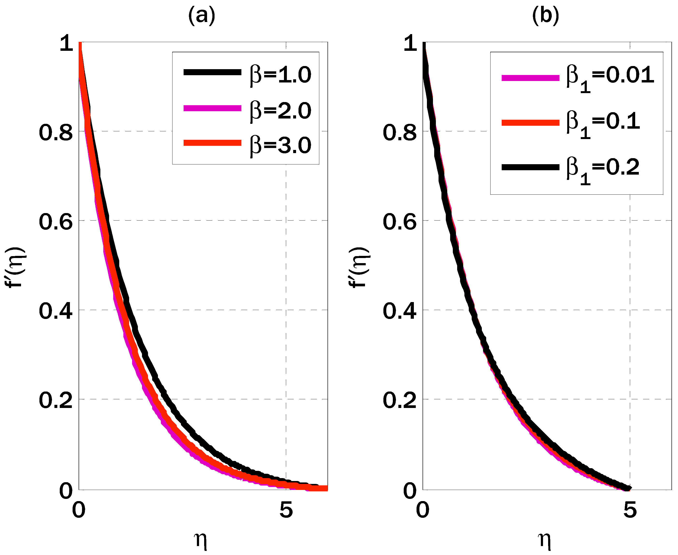
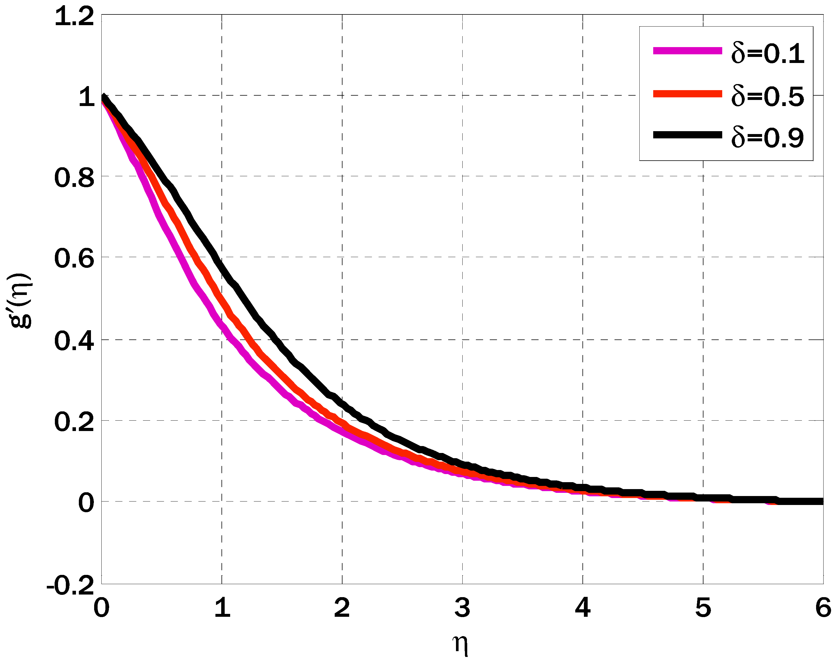
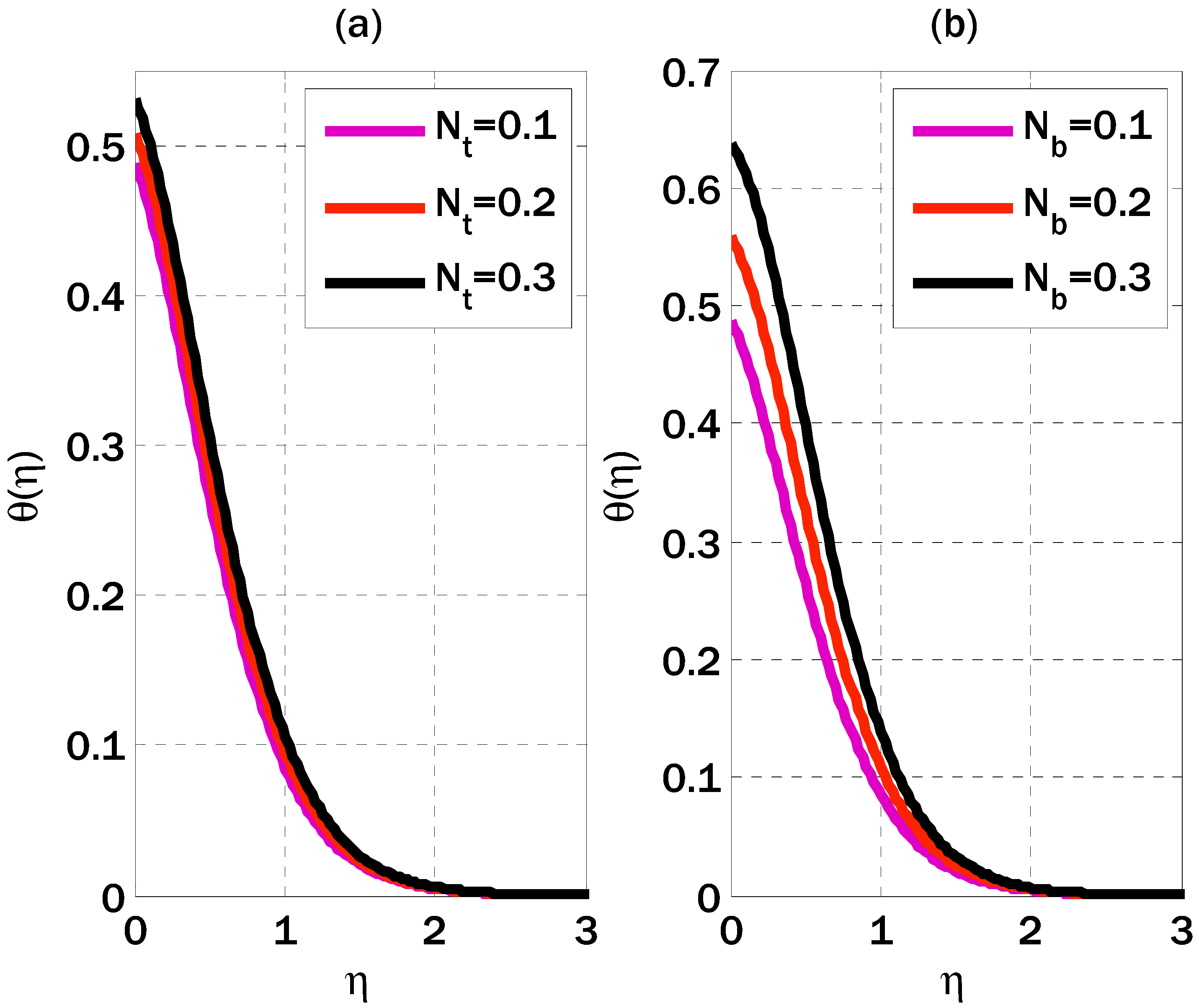
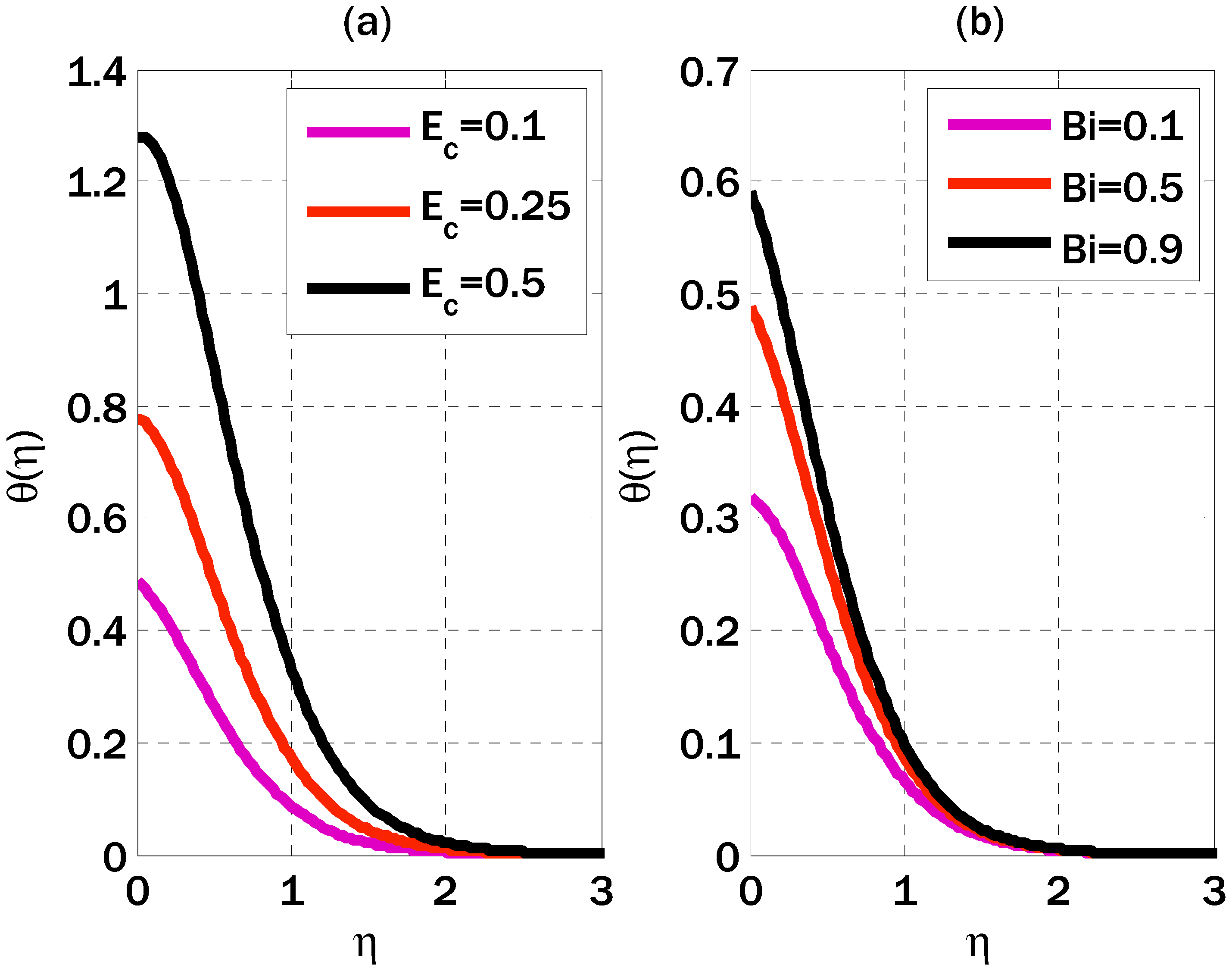
The impact of the electric field parameter and magnetic parameter M on the velocity profile is displayed in Figure 1. Figure 1 shows that the velocity increased by enhancing the electric field parameter d . It decayed by increasing the magnetic parameter M . The reason behind the enhancement of velocity was the consequence of increasing the Lorentz force that resisted the velocity of the flow. The rise in the Lorentz force occurred due to a growth in the magnetic parameter M . Figure 2 portrays the effect of the Casson parameter and magnetic parameter β 1 . The velocity profile decayed by increasing the Casson parameter, which had a dual behavior due to the growing values of the magnetic parameter β . Since the coefficient of the diffusion term decreased by incrementing the Casson parameter, this led to a decay in the velocity profile. The effect of the reciprocal of the magnetic Prandtl number on the horizontal component of the induced magnetic field is displayed in Figure 3. The horizontal component of the induced magnetic field escalated by increasing the reciprocal of the magnetic Prandtl number. Figure 4 displays the temperature curve as a function of the thermophoresis and Brownian motion parameters. The temperature profile escalated by incrementing thermophoresis and Brownian motion parameters. The increase in the temperature profile due to the escalation of the thermophoresis parameter was due to the incrementing thermophoresis force as hot particles of the fluid shifted in the vicinity while cold particles moved closer to the plate. Additionally, the escalation of the Brownian motion parameter increased the process of randomly shifting particles; therefore, the temperature spread in the nearby regions, resulting in the growth of the temperature profile. Figure 5 shows the effect of the Eckert number and Biot number on the temperature profile. The temperature profile escalates by growing Eckert and Biot numbers. Since internal friction between the particles increased due to the rising Eckert number; therefore, the temperature profile was boosted. Figure 6 shows the concentration curve as a function of the Schmidt number and the reaction rate parameter. Growing values of the Schmidt number and the dimensionless reaction rate parameter decayed the concentration profile. Since mass diffusivity and Schmidt number were inversely proportional to each other, the mass diffusivity decayed due to the rising Schmidt number values, leading to a decay in the concentration profile. The numerical values of the parameters in this research were chosen randomly, or these numerical values of the parameters depended on the behavior of the profiles. However, in real-world applications, these values depended on the physical behavior of different boundary layers over the flat plates.
In Table 1, we can see how the results of the proposed system compare to those of previous studies. The obtained results have some resemblance with those given in past research. It can be observed from Table 1 that the results obtained by the proposed scheme were accurate up to the second digits after the decimal points. Table 2 shows the numerical values for the skin friction coefficient by varying local electric parameters, the magnetic parameter M , Casson parameters, and the magnetic parameter β 1 . The skin friction coefficient declined due to the growing values of magnetic parameters and rose by escalating the local electric parameter and Casson parameter. The local Nusselt number, as a function of the Eckert number, thermophoresis, the Brownian motion parameter, the Biot number, and the Prandtl number, are listed in Table 3. The Eckert number, the Brownian motion parameter, and the Biot number decreased as the Prandtl number, the thermophoresis parameter, and the local Nusselt number increased. The local Sherwood number was affected by the thermophoresis parameter, Brownian motion parameter, Schmidt number, and response rate parameter, as shown in Table 4. As the thermophoresis parameter was raised, the local Sherwood number fell, and during the Brownian motion parameter, the Schmidt number and reaction rate parameter all increased.
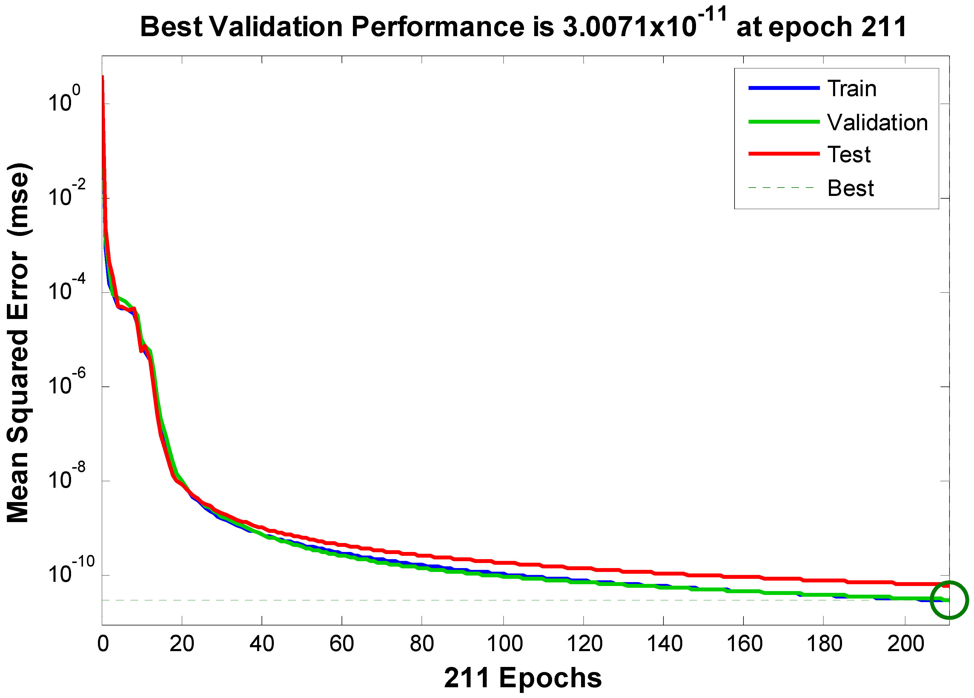
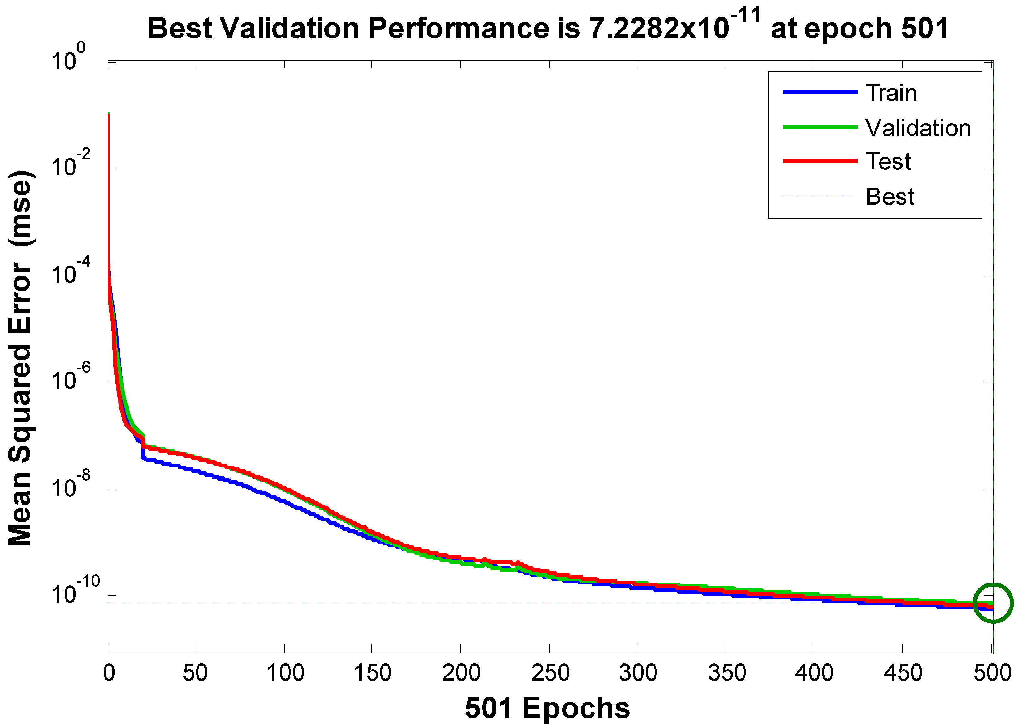
This contribution also consisted of the neural network approach that mapped between a data set and a set of numerical targets. The neural network fitting tool helped to create and train a network and select data, which helped evaluate its performance using regression analysis and means square error. The Levenberg–Marquardt backpropagation algorithm was utilized by training a network and scaled conjugate gradient backpropagation, which could be utilized if there was insufficient memory. The Levenberg–Marquardt algorithm could be employed to solve non-linear least square problems. It interpolated between the gradient descent method and the Gauss–Newton algorithm. In some particular cases, it is slower than the Gauss–Newton algorithm. If there existed more than one minimum, then it could only find a local minimum, and this local minimum was not necessarily the global minimum. Additionally, if the initial was close to the final solution, it converged to the global minimum for the problem with multiple minima. The mathematical model for this contribution had one input and four outputs. The four targets were the velocity profile, x -component of the induced magnetic field, temperature profile, and concentration profile. The neural network approach was applied to three targets from these four targets. Two hundred points were used, among which 140 samples were used for training, 30 for validation, and 30 for testing. Figure 7, Figure 8 and Figure 9 show the mean square error over epochs. The mean square error can be computed from the following formula:
M S E = 1 N j = 1 N X p r e d j X t a r g j 2
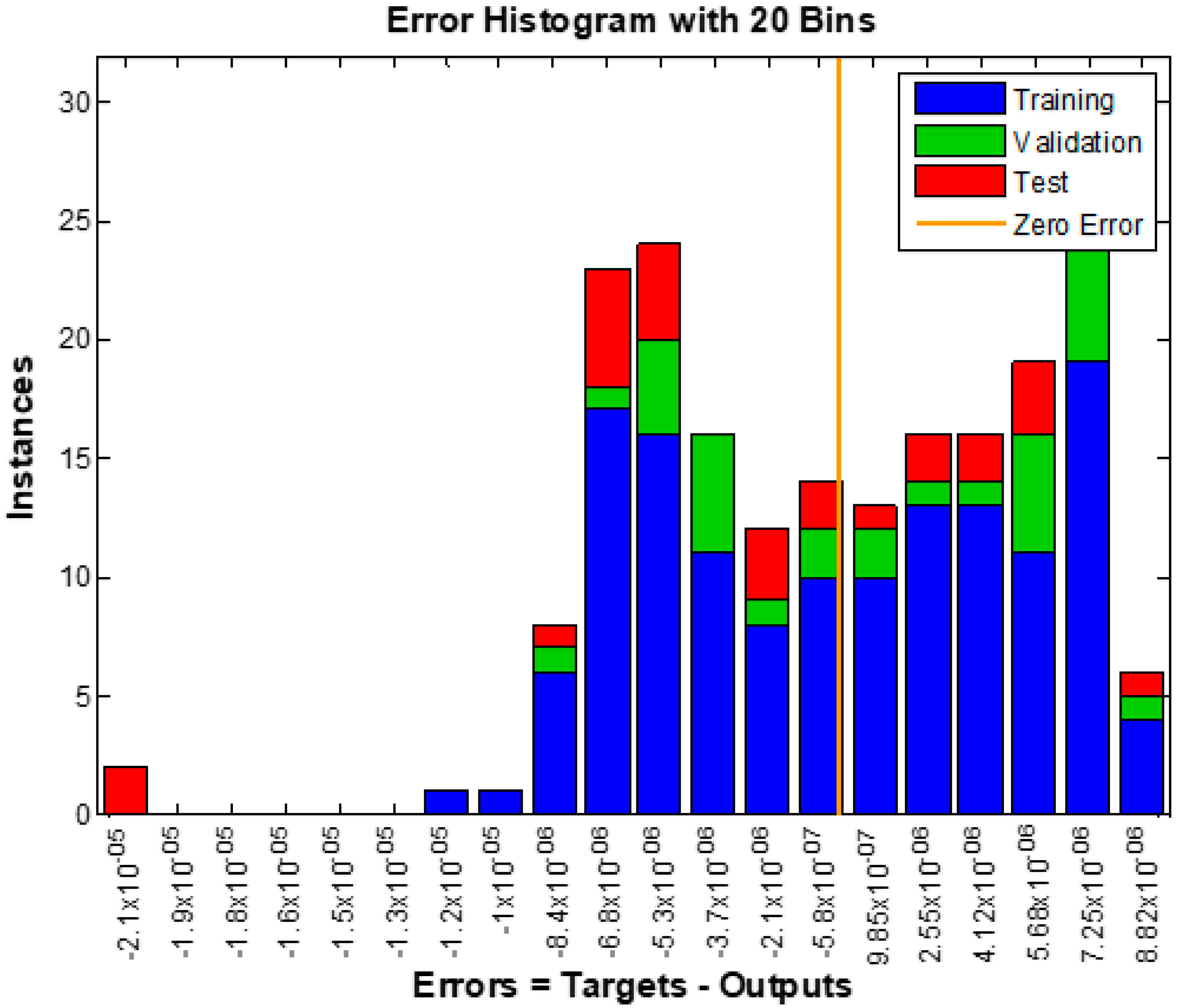
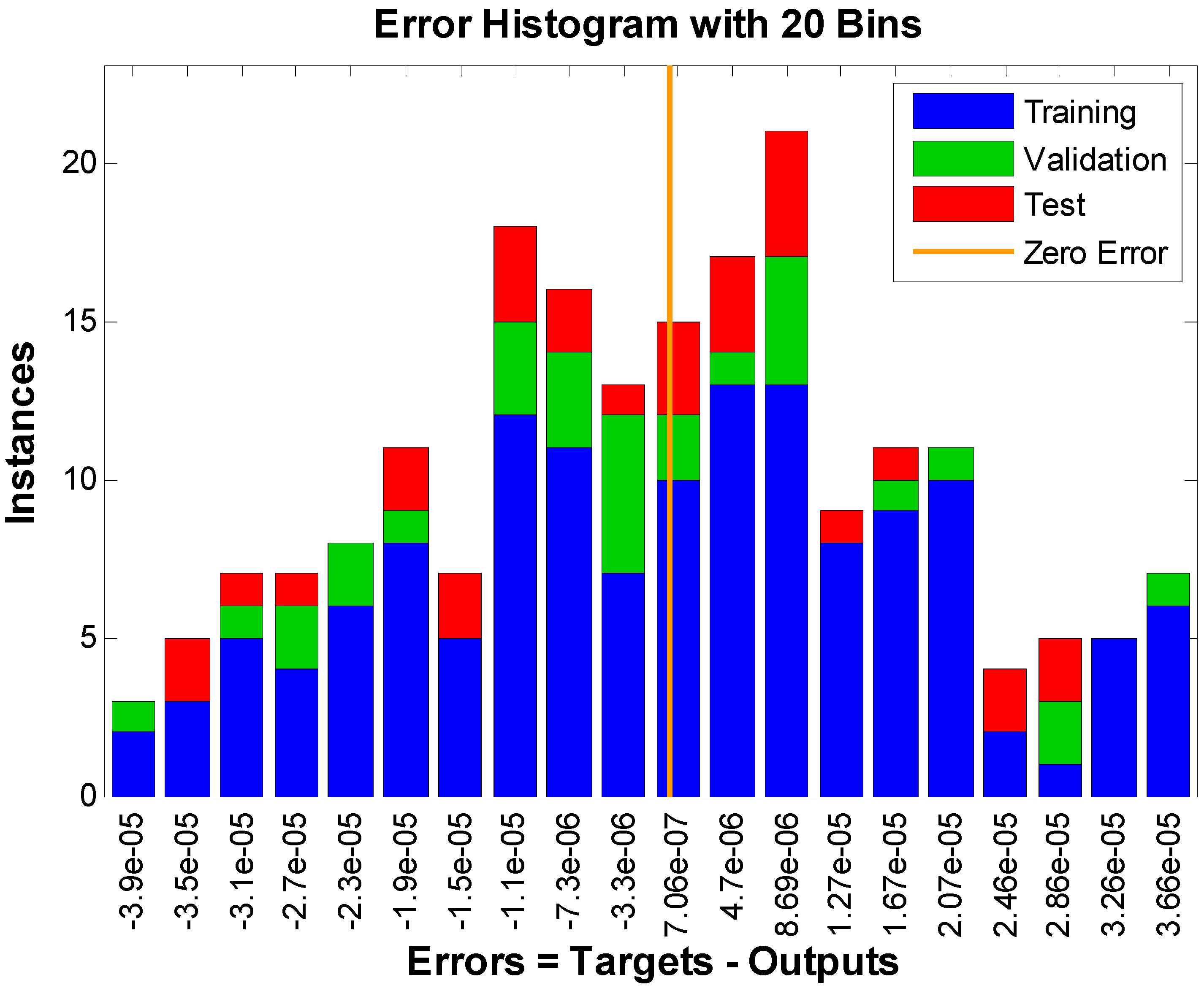
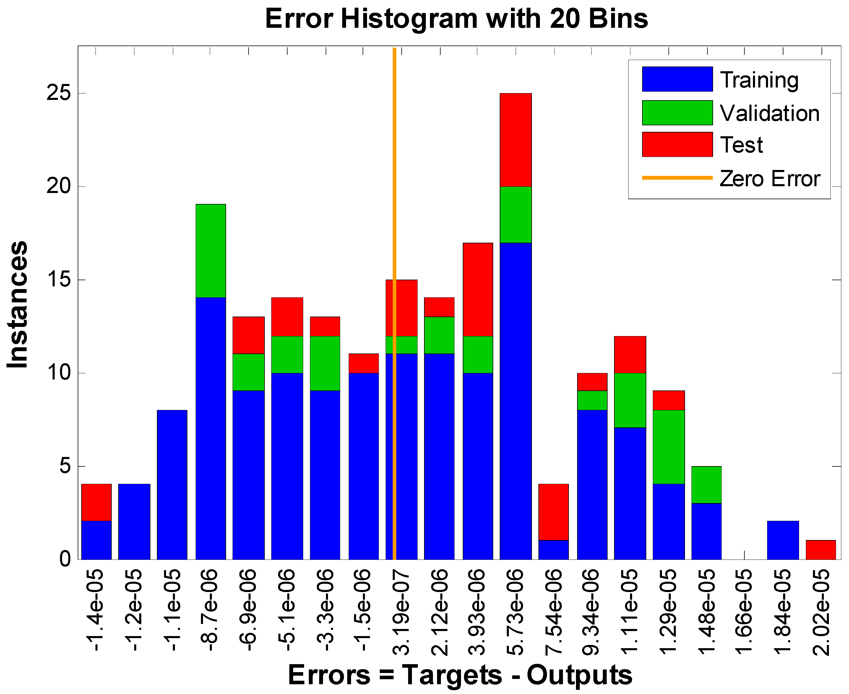
The best performance was achieved at the last epoch for all the velocity, temperature, and concentration profile targets. Figure 10, Figure 11 and Figure 12 show the error histogram for the velocity, temperature, and concentration profiles as targets. These error histograms show how many samples give a certain amount of error. The zero error was the minimum error that was achieved. The error was found as:
E r r o r = X t a r g X p r e d
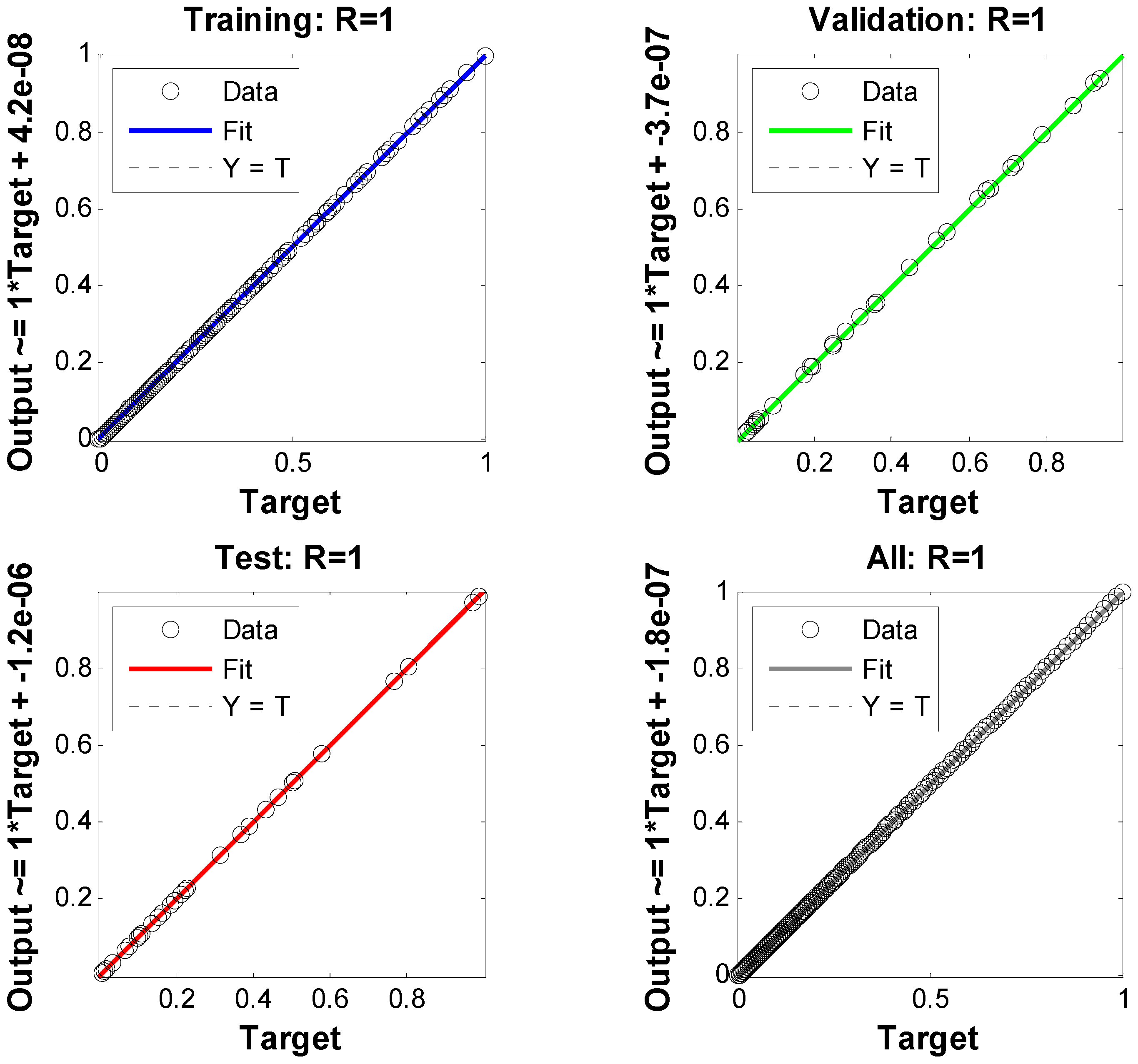
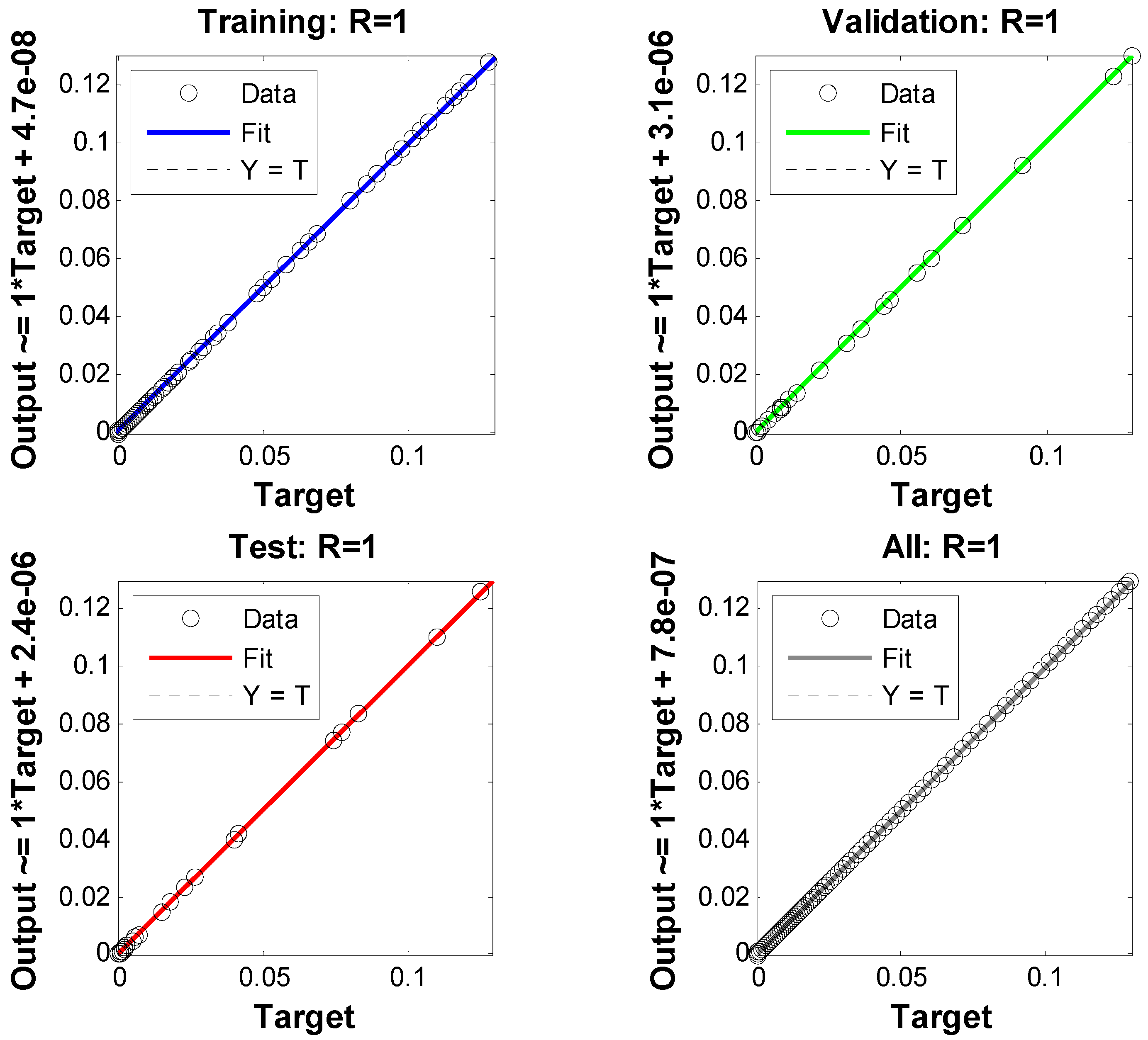
where X p r e d is the output. So, the error histogram found the error, which is the difference between the targeted and output values for velocity, temperature, and concentration profiles. Figure 13, Figure 14 and Figure 15 show the regression analysis of output or predicted and targeted values. The following regression line was fitted to draw Figure 13, Figure 14 and Figure 15,
Y p r e d = X t a r g + ε
Figure 16 shows the correlation between the input and error. The error was the difference between the output and target of the velocity profile.

7. Conclusions

This study used artificial neural networks backpropagated with the Levenberg–Marquardt method to examine the effects of factors of interest on velocity and temperature profiles in the suggested fluid flow system. This made it possible to evaluate the impact of an induced magnetic field on heat and mass transfer in a non-Newtonian Casson nanofluid flow. Neural network modeling provided a different way to study the relationship between the input and targets. The targets in the form of velocity, temperature and concentration profiles could be obtained by applying the proposed scheme to the given model of the fluid flow problem. The regression plots showed how accurately the output was obtained using the adopted approach. The neural network technique is currently used on three of these four targets. Two hundred points were utilized, with 140 samples used for training, 30 samples used for validation, and 30 samples used for testing. These findings demonstrate the efficacy of artificial neural networks when forecasting and optimizing complex systems. This work also provided an explicit numerical scheme that was third-order accurate. This scheme consisted of two stages. The order of accuracy of the scheme could be proved from its construction analysis. Since the scheme was capable only of initial value problems, a shooting method was applied to solve the boundary value problems. The shooting method was based on the Matlab solver fsolve for solving equations, and the proposed scheme was employed to solve differential equations. The concluding points can be summarized as:
  • The proposed scheme was third-order accurate in two stages.
  • As the Casson parameter increased, the velocity profile slowed down, and as the magnetic parameter β increased, it displayed a dual behavior.
  • Growing values of the reciprocal of the magnetic Prandtl number raised the horizontal component of the induced magnetic field.
  • Three models representing velocity, temperature, and concentration profiles were implemented using a neural network approach.
The proposed numerical scheme could solve various partial differential equations commonly encountered in science and engineering. Upon the conclusion of this study, it is feasible to suggest alternative applications for the present methods in conjunction with their existing uses [42,43,44,45]. Furthermore, the suggested approach is user-friendly and has the potential to be utilized when resolving a wider range of partial differential equations in the fields of science and engineering.

Author Contributions

Conceptualization, methodology, and analysis, Y.N.; funding acquisition, K.A.; investigation, Y.N.; methodology, M.S.A.; project administration, K.A.; resources, K.A.; supervision, M.S.A.; visualization, K.A.; writing—review and editing, M.S.A.; proofreading and editing, M.S.A. All authors have read and agreed to the published version of the manuscript.

Funding

This research received no external funding.

Data Availability Statement

The manuscript included all required data and implementing information.

Acknowledgments

The authors wish to express their gratitude to Prince Sultan University for facilitating the publication of this article through the Theoretical and Applied Sciences Lab.

Conflicts of Interest

The authors declare no conflict of interest.

Nomenclature

u Horizontal components of velocity ( m · S 1 ) σ Electrical conductivity of the fluid S · m 1
y Cartesian co-ordinate m T Temperature of fluid K
ν Kinematic viscosity m 2 · s 1 T w Temperature of fluid at the wall K
ρ Density of fluid k g · m 3 T Ambient temperature of the fluid K
C Concentration of fluid m o l · m 3 C w Concentration on the wall m o l · m 3
D B Brownian diffusion coefficient m 2 · s 1 C Ambient concentration m o l · m 3
c p Specific heat capacity J · k g 1 · K 1 D T Thermophoresis coefficient m 2 · s 1
H x Horizontal component of induced magnetic field A · m 1 H y Vertical component of induced magnetic field A · m 1
γ Reaction rate α Thermal diffusivity m 2 · s 1
k 1 Reaction rate parameter s 1 μ Dynamic viscosity k g · m 1 · s 1
Γ Time constant (s) τ Effective heat capacity of fluid
α 1 Magnetic diffusivity m 2 · s 1 E c Eckert number
P r Prandtl number N t Thermophoresis variable
N b Brownian motion variable S c Schmidt number
β Magnetic parameter W e Weissenberg number
δ Reciprocal of magnetic Prandtl number M Magnetic parameter
E 1 local electric parameter B i Biot number

References

  1. Casson, N. A flow equation for pigment-oil suspensions of the printing ink type. In Rheology of Disperse Systems; Mill, C.C., Ed.; Pergamon Press: Oxford, UK, 1959; pp. 84–104. [Google Scholar]
  2. Mustafa, M.; Hayat, T.; Ioan, P.; Hendi, A. Stagnation-point flow and heat transfer of a Casson fluid towards a stretching sheet. Z. Für Nat. A 2012, 67, 70–76. [Google Scholar] [CrossRef]
  3. Mukhopadhyay, S. Casson fluid flow and heat transfer over a nonlinearly stretching surface. Chin. Phys. B 2013, 22, 074701. [Google Scholar] [CrossRef]
  4. Mukhopadhyay, S.; Mondal, I.C.; Chamkha, A.J. Casson fluid flow and heat transfer past a symmetric wedge. Heat Transf. Asian Res. 2013, 42, 665–675. [Google Scholar] [CrossRef]
  5. Pramanik, S. Casson fluid flow and heat transfer past an exponentially porous stretching surface in presence of thermal radiation. Ain Shams Eng. J. 2014, 5, 205–212. [Google Scholar] [CrossRef]
  6. Mahdy, A. Heat transfer and flow of a Casson fluid due to a stretching cylinder with the Soret and Dufour effects. J. Eng. Phys. Thermophys. 2015, 88, 928–936. [Google Scholar] [CrossRef]
  7. Abbas, Z.; Sheikh, M.; Motsa, S.S. Numerical solution of binary chemical reaction on stagnation point flow of Casson fluid over a stretching/shrinking sheet with thermal radiation. Energy 2016, 95, 12–20. [Google Scholar] [CrossRef]
  8. Raju, C.S.K.; Hoque, M.M.; Sivasankar, T. Radiative flow of Casson fluid over a moving wedge filled with gyrotactic microorganisms. Adv. Powder Technol. 2017, 28, 575–583. [Google Scholar] [CrossRef]
  9. Reddy, G.J.; Kethireddy, B.; Umavathi, J.C.; Sheremet, M.A. Heat flow visualization for unsteady Casson fluid past a vertical slender hollow cylinder. Ther. Sci. Eng. Prog. 2018, 5, 172–181. [Google Scholar] [CrossRef]
  10. Sulochana, C.; Ashwinkumar, G.P.; Sandeep, N. Effect of frictional heating on mixed convection flow of chemically reacting radiative Casson nanofluid over an inclined porous plate. Alex. Eng. J. 2018, 57, 2573–2584. [Google Scholar] [CrossRef]
  11. Ali, A.; Umar, M.; Bukhari, Z.; Abbas, Z. Pulsating flow of a micropolar-Casson fluid through a constricted channel influenced by a magnetic field and Darcian porous medium: A numerical study. Results Phys. 2020, 19, 103544. [Google Scholar] [CrossRef]
  12. Rehman, K.U.; Shatanawi, W.; Çolak, A.B. Artificial Neural Networking Magnification for Heat Transfer Coefficient in Convective Non-Newtonian Fluid with Thermal Radiations and Heat Generation Effects. Mathematics 2023, 11, 342. [Google Scholar] [CrossRef]
  13. Alizadeh, R.; Gomari, S.R.; Alizadeh, A.; Karimi, N.; Li, L.K. Combined heat and mass transfer and thermodynamic irreversibilities in the stagnation-point flow of Casson rheological fluid over a cylinder with catalytic reactions and inside a porous medium under local thermal nonequilibrium. Comput. Math. Appl. 2021, 81, 786–810. [Google Scholar] [CrossRef]
  14. Jamshed, W.; Goodarzi, M.; Prakash, M.; Nisar, K.S.; Zakarya, M.; Abdel-Aty, A.H. Evaluating the unsteady Casson nanofluid over a stretching sheet with solar thermal radiation: An optimal case study. Case Stud. Therm. Eng. 2021, 26, 101160. [Google Scholar] [CrossRef]
  15. Rehman, K.U.; Shatanawi, W.; Yaseen, S. A Comparative Numerical Study of Heat and Mass Transfer Individualities in Casson Stagnation Point Fluid Flow Past a Flat and Cylindrical Surfaces. Mathematics 2023, 11, 470. [Google Scholar] [CrossRef]
  16. Shatnawi, T.A.; Abbas, N.; Shatanawi, W. Mathematical analysis of unsteady stagnation point flow of radiative Casson hybrid nanofluid flow over a vertical Riga sheet. Mathematics 2022, 10, 3573. [Google Scholar] [CrossRef]
  17. Awan, A.U.; Ahammad, N.A.; Shatanawi, W.; Allahyani, S.A.; Tag-ElDin, E.M.; Abbas, N.; Ali, B. Significance of magnetic field and Darcy–Forchheimer law on dynamics of Casson-Sutterby nanofluid subject to a stretching circular cylinder. Int. Commun. Heat Mass Transf. 2022, 139, 106399. [Google Scholar] [CrossRef]
  18. Nawaz, Y.; Arif, M.S.; Abodayeh, K. Predictor–Corrector Scheme for Electrical Magnetohydrodynamic (MHD) Casson Nanofluid Flow: A Computational Study. Appl. Sci. 2023, 13, 1209. [Google Scholar] [CrossRef]
  19. Ly, H.B.; Nguyen, M.H.; Pham, B.T. Metaheuristic optimization of Levenberg-Marquardt-based artificial neural network using particle swarm optimization for prediction of foamed concrete compressive strength. Neural Comput. Appl. 2021, 33, 17331–17351. [Google Scholar] [CrossRef]
  20. Zhao, J.; Nguyen, H.; Nguyen-Thoi, T.; Asteris, P.G.; Zhou, J. Improved Levenberg-Marquardt backpropagation neural network by particle swarm and whale optimization algorithms to predict the deflection of RC beams. Eng. Comput. 2022, 38, 3847–3869. [Google Scholar] [CrossRef]
  21. Nguyen, H.X.; Cao, H.Q.; Nguyen, T.T.; Tran, T.N.C.; Tran, H.N.; Jeon, J.W. Improving robot precision positioning using a neural network based on Levenberg Marquardt–APSO algorithm. IEEE Access 2021, 9, 75415–75425. [Google Scholar] [CrossRef]
  22. Ali, M.S.; Ayaz, M.; Mansoor, T. Prediction of discharge through a sharp-crested triangular weir using ANN model trained with Levenberg-Marquardt algorithm, model. Earth Syst. Environ. 2022, 8, 1405–1417. [Google Scholar] [CrossRef]
  23. Ye, Z.; Kim, M.K. Predicting electricity consumption in a building using an optimized backpropagation and Levenberg-Marquardt backpropagation neural network: Case study of a shopping mall in China, Sustain. Cities Soc. 2018, 42, 176–183. [Google Scholar] [CrossRef]
  24. Bharati, S.; Rahman, M.A.; Podder, P.; Robel, M.R.A.; Gandhi, N. Comparative performance analysis of neural network base training algorithm and neuro-fuzzy system with SOM for the purpose of prediction of the features of superconductors. In International Conference on Intelligent Systems Design and Applications, Advances in Intelligent Systems and Computing; Springer: Cham, Switzerland, 2019; Volume 1181, pp. 69–79. [Google Scholar] [CrossRef]
  25. Shoaib, M.; Zubair, G.; Nisar, K.S.; Raja, M.A.Z.; Khan, M.I.; Gowda, R.P.; Prasannakumara, B. Ohmic heating effects and entropy generation for nanofluidic system of Ree-Eyring fluid: Intelligent computing paradigm. Int. Commun. Heat Mass Transf. 2021, 129, 105683. [Google Scholar] [CrossRef]
  26. Ahmad, I.; Ilyas, H.; Raja, M.A.Z.; Khan, Z.; Shoaib, M. Stochastic numerical computing with Levenberg-Marquardt backpropagation for performance analysis of heat Sink of functionally graded material of the porous fin. Surf. Interfaces 2021, 26, 101403. [Google Scholar] [CrossRef]
  27. Shoaib, M.; Raja, M.A.Z.; Sabir, M.T.; Bukhari, A.H.; Alrabaiah, H.; Shah, Z.; Kumam, P.; Islam, S. A stochastic numerical analysis based on hybrid NAR-RBFs networks non-linear SITR model for novel COVID-19 dynamics. Comput. Methods Programs Biomed. 2021, 202, 105973. [Google Scholar] [CrossRef]
  28. Shafiq, A.; Çolak, A.B.; Sindhu, T.N.; Al-Mdallal, Q.M.; Abdeljawad, T. Estimation of unsteady hydromagnetic Williamson fluid flow in a radiative surface through numerical and artificial neural network modeling. Sci. Rep. 2021, 11, 14509. [Google Scholar] [CrossRef] [PubMed]
  29. Shafiq, A.; Çolak, A.B.; Naz Sindhu, T. Designing artificial neural network of nanoparticle diameter and solid–fluid interfacial layer on single walled carbon nanotubes/ethylene glycol nanofluid flow on thin slendering needles. Int. J. Numer. Methods Fluids 2021, 93, 3384–3404. [Google Scholar] [CrossRef]
  30. Sabir, Z.; Raja, M.A.Z.; Guirao, J.L.; Shoaib, M. Integrated intelligent computing with neuroswarming solver for multi-singular fourth-order non-linear Emden–Fowler equation. Comput. Appl. Math. 2020, 39, 307. [Google Scholar] [CrossRef]
  31. Sabir, Z.; Raja, M.A.Z.; Umar, M.; Shoaib, M. Neuro-swarm intelligent computing to solve the second-order singular functional differential model. Eur. Phys. J. Plus 2020, 135, 474. [Google Scholar] [CrossRef]
  32. Shafiq, A.; Çolak, A.B.; Sindhu, T.N.; Muhammad, T. Optimization of Darcy-Forchheimer squeezing flow in non-linear stratified fluid under convective conditions with artificial neural network. Heat Transf. Res. 2022, 53, 67–89. [Google Scholar] [CrossRef]
  33. Shoaib, M.; Kausar, M.; Nisar, K.S.; Raja, M.A.Z.; Zeb, M.; Morsy, A. The design of intelligent networks for entropy generation in Ree-Eyring dissipative fluid flow system along quartic autocatalysis chemical reactions. Int. Commun. Heat Mass Transf. 2022, 133, 105971. [Google Scholar] [CrossRef]
  34. Umar, M.; Raja, M.A.Z.; Sabir, Z.; Alwabli, A.S.; Shoaib, M. A stochastic computational intelligent solver for numerical treatment of mosquito dispersal model in a heterogeneous environment. Eur. Phys. J. Plus 2020, 135, 565. [Google Scholar] [CrossRef]
  35. Abodayeh, K.; Raza, A.; Arif, M.S.; Rafiq, M.; Bibi, M.; Mohsin, M. Stochastic numerical analysis for impact of heavy alcohol consumption on transmission dynamics of gonorrhoea epidemic. CMC-Comput. Mater. Contin. 2020, 62, 1125–1142. [Google Scholar] [CrossRef]
  36. Shoaib Arif, M.; Raza, A.; Abodayeh, K.; Rafiq, M.; Bibi, M.; Nazeer, A. A numerical efficient technique for the solution of susceptible infected recovered epidemic model. Comput. Model. Eng. Sci. 2020, 124, 477–491. [Google Scholar] [CrossRef]
  37. Raza, A.; Rafiq, M.; Baleanu, D.; Shoaib Arif, M.; Naveed, M.; Ashraf, K. Competitive numerical analysis for stochastic HIV/AIDS epidemic model in a two-sex population. IET Syst. Biol. 2019, 13, 305–315. [Google Scholar] [CrossRef] [PubMed]
  38. Umar, M.; Amin, F.; Al-Mdallal, Q.; Ali, M.R. A stochastic computing procedure to solve the dynamics of prevention in HIV system. Biomed. Signal Process. Control 2022, 78, 103888. [Google Scholar] [CrossRef]
  39. Sajjad, U.; Hussain, I.; Imran, M.; Sultan, M.; Wang, C.-C.; Alsubaie, A.S.; Mahmoud, K.H. Boiling Heat Transfer Evaluation in Nanoporous Surface Coatings. Nanomaterials 2021, 11, 3383. [Google Scholar] [CrossRef]
  40. Yih, K.A. Free convection effect on MHD coupled heat and mass transfer of a moving permeable vertical surface. Int. Commun. Heat Mass Transf. 1999, 26, 95–104. [Google Scholar] [CrossRef]
  41. Hayat, T.; Mustafa, M.; Pop, I. Heat and mass transfer for Soret and Dufour’s effect on mixed convection boundary layer flow over a stretching vertical surface in a porous medium filled with a viscoelastic fluid. Commun. Non-Linear Sci. Numer. Simul. 2010, 15, 1183–1196. [Google Scholar] [CrossRef]
  42. Nawaz, Y.; Arif, M.S.; Abodayeh, K.; Bibi, M. Finite Element Method for Non-Newtonian Radiative Maxwell Nanofluid Flow under the Influence of Heat and Mass Transfer. Energies 2022, 15, 4713. [Google Scholar] [CrossRef]
  43. Arif, M.S.; Abodayeh, K.; Nawaz, Y. A Reliable Computational Scheme for Stochastic Reaction–Diffusion Non-linear Chemical Model. Axioms 2023, 12, 460. [Google Scholar] [CrossRef]
  44. Arif, M.S.; Shatanawi, W.; Nawaz, Y. A numerical scheme for Darcy-Forchheimer flow of non-Newtonian nanofluid under the effects of convective and zero mass flux boundary conditions. Ther. Sci. 2023. [Google Scholar] [CrossRef]
  45. Arif, M.S.; Abodayeh, K.; Nawaz, Y. A Computational Scheme for Stochastic Non-Newtonian Mixed Convection Nanofluid Flow over Oscillatory Sheet. Energies 2023, 16, 2298. [Google Scholar] [CrossRef]
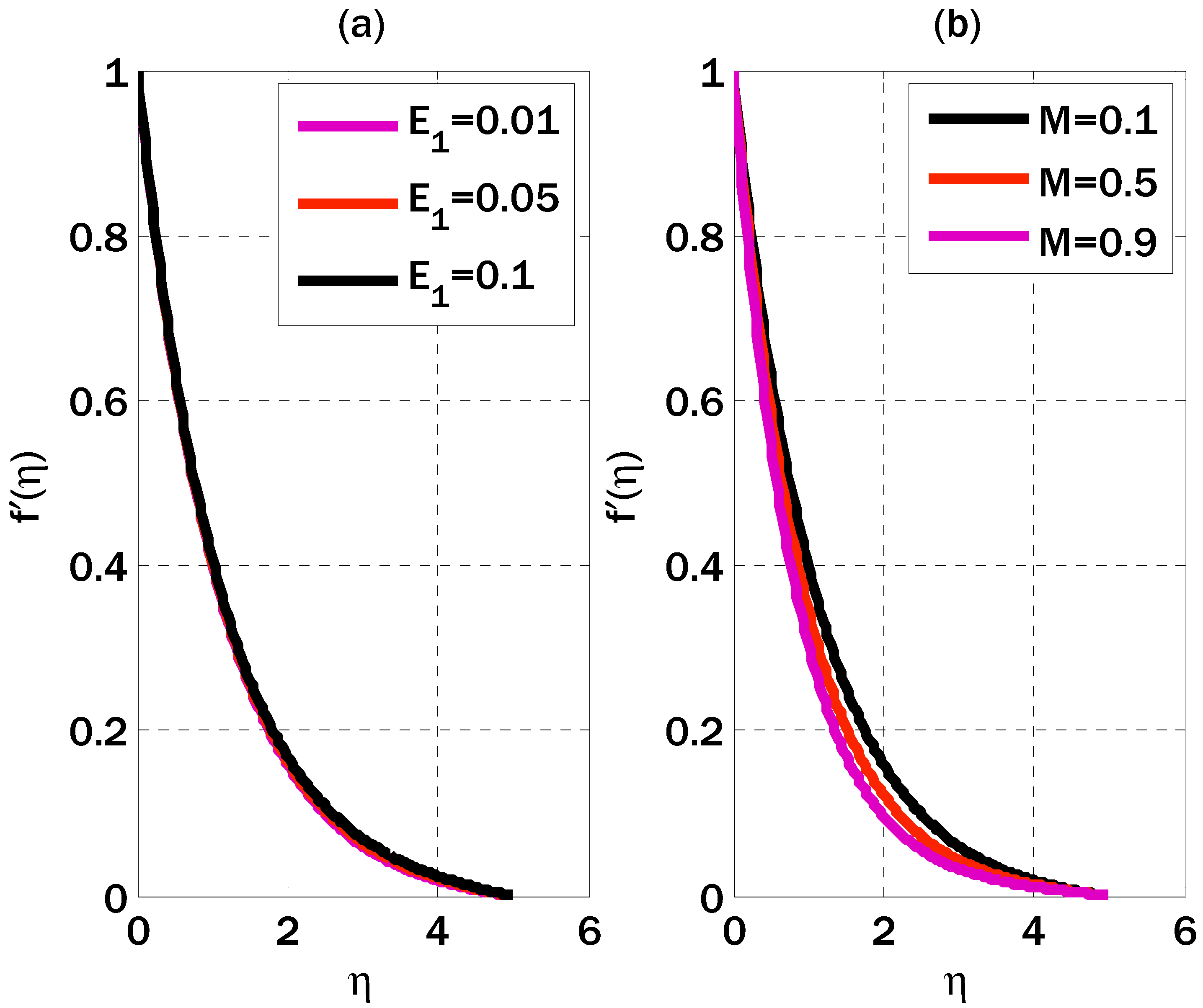
Figure 1. Variation in electric field parameter and magnetic parameter M on velocity profile using β 1 = 0.01 , β = 3 , δ = 1.5 (a) M = 0.1 (b) E 1 = 0.01 .
Axioms 12 00527 g001
Figure 2. Variation in the Casson parameter and magnetic parameter β 1 on the velocity profile using E 1 = 0.01 , M = 0.2 , δ = 1.5 (a) β 1 = 0.01 (b) β = 1 .
Axioms 12 00527 g002
Figure 3. Variation in the reciprocal of magnetic Prandtl number on the horizontal component of the induced magnetic field using E 1 = 0.01 , M = 0.1 , β 1 = 0.01 , β = 3 .
Axioms 12 00527 g003
Figure 4. Variation in thermophoresis and Brownian motion parameters on the temperature profile using, E 1 = 0.01 , M = 0.9 , β 1 = 0.01   β = 3 , E c = 0.1 , B i = 0.5 , δ = 1.5 , P r = 5 , S c = 1.5 , γ = 1 (a) N b = 0.1 (b) N t = 0.1 .
Axioms 12 00527 g004
Figure 5. Variation in the Eckert number and Biot number on temperature profile using, E 1 = 0.01 , M = 0.9 , β 1 = 0.01   β = 3 , N t = 0.1 , N b = 0.1 , δ = 1.5 , P r = 5 , S c = 1.5 , γ = 1 (a) B i = 0.5 (b) E c = 0.1 .
Axioms 12 00527 g005
Figure 6. Variation in the Schmidt number and reaction rate parameter on concentration profiles using, E 1 = 0.01 , M = 0.9 , β 1 = 0.01   β = 3 , N t = 0.1 , N b = 0.1 , δ = 1.5 , P r = 5 , E c = 0.1 , B i = 0.1 (a) γ = 1 (b) S c = 1.5 .
Axioms 12 00527 g006
Figure 7. Training performance for the target of using the velocity profile, E 1 = 0.01 , M = 0.1 , β 1 = 0.05 , β = 0.7 , N t = 0.01 , N b = 0.01 , δ = 1.5 , P r = 5 , E c = 0.1 , B i = 0.1 , γ = 0.9 , S c = 1.5 .
Axioms 12 00527 g007
Figure 8. Training performance for the target of using temperature profile E 1 = 0.01 , M = 0.1 , β 1 = 0.05 , β = 0.7 , N t = 0.01 , N b = 0.01 , δ = 1.5 , P r = 5 , E c = 0.1 , B i = 0.1 , γ = 0.9 , S c = 1.5 .
Axioms 12 00527 g008
Figure 9. Training performance for the target of using a concentration profile E 1 = 0.01 , M = 0.1 , β 1 = 0.05 , β = 0.7 , N t = 0.01 , N b = 0.01 , δ = 1.5 , P r = 5 , E c = 0.1 , B i = 0.1 , γ = 0.9 , S c = 1.5 .
Axioms 12 00527 g009
Figure 10. Error from using the target of velocity profile E 1 = 0.01 , M = 0.1 , β 1 = 0.05 , β = 0.7 , N t = 0.01 , N b = 0.01 , δ = 1.5 , P r = 5 , E c = 0.1 , B i = 0.1 , γ = 0.9 , S c = 1.5 .
Axioms 12 00527 g010
Figure 11. Error histogram from using the target of temperature profile E 1 = 0.01 , M = 0.1 , β 1 = 0.05 , β = 0.7 , N t = 0.01 , N b = 0.01 , δ = 1.5 , P r = 5 , E c = 0.1 , B i = 0.1 , γ = 0.9 , S c = 1.5 .
Axioms 12 00527 g011
Figure 12. Error histogram from using the target of concentration profile E 1 = 0.01 , M = 0.1 , β 1 = 0.05 , β = 0.7 , N t = 0.01 , N b = 0.01 , δ = 1.5 , P r = 5 , E c = 0.1 , B i = 0.1 , γ = 0.9 , S c = 1.5 .
Axioms 12 00527 g012
Figure 13. Regression analysis from using the target of the velocity profile E 1 = 0.01 , M = 0.1 , β 1 = 0.05 , β = 0.7 , N t = 0.01 , N b = 0.01 , δ = 1.5 , P r = 5 , E c = 0.1 , B i = 0.1 , γ = 0.9 , S c = 1.5 .
Axioms 12 00527 g013
Figure 14. Regression analysis from using the target of temperature profile E 1 = 0.01 , M = 0.1 , β 1 = 0.05 , β = 0.7 , N t = 0.01 , N b = 0.01 , δ = 1.5 , P r = 5 , E c = 0.1 , B i = 0.1 , γ = 0.9 , S c = 1.5 .
Axioms 12 00527 g014
Figure 15. Regression analysis from using the target of concentration profile E 1 = 0.01 , M = 0.1 , β 1 = 0.05 , β = 0.7 , N t = 0.01 , N b = 0.01 , δ = 1.5 , P r = 5 , E c = 0.1 , B i = 0.1 , γ = 0.9 , S c = 1.5 .
Axioms 12 00527 g015
Figure 16. Correlation between input error, output and target (velocity profile) using E 1 = 0.01 , M = 0.1 , β 1 = 0.05 , β = 0.7 , N t = 0.01 , N b = 0.01 , δ = 1.5 , P r = 5 , E c = 0.1 , B i = 0.1 , γ = 0.9 , S c = 1.5 .
Axioms 12 00527 g016
Table 1. Verification of some results obtained by the proposed scheme using E 1 = 0 , β , β 1 = 0.1 , δ .
M Yih [40]Hayat et al. [41]Proposed
0.0 1.0000 1.000000 1.0009
0.5 1.2247 1.224747 1.2231
1.0 1.4142 1.414217 1.4108
1.5 1.5811 1.581147 1.5815
2.0 1.7321 1.732057 1.7360
Table 2. List of numerical values for the skin friction coefficient using δ = 1.5 .
E 1 M β β 1 R e 1 / 2 C f
0.01 0.1 0.7 0.01 1.6578
0.05 1.6521
0.01 0.5 1.9152
0.1 1.0 1.4984
0.7 0.05 1.6744
Table 3. List of numerical values for the local Nusselt number using β = 0.7 , β 1 = 0.05 , E 1 = 0.01 , M = 0.1 , δ = 1.5 , S c = 1.5 , γ = 0.1 .
E c N t N b B i P r R e 1 / 2 N u x
0.1 0.01 0.01 0.1 5 0.0870
0.5 0.0589
0.1 0.05 0.0871
0.01 0.05 0.0865
0.01 0.5 0.3523
0.1 7 0.0873
Table 4. List of numerical values for local Sherwood number using β = 0.7 , β 1 = 0.05 , E 1 = 0.01 , M = 0.1 , δ = 1.5 , P r = 5 , E c = 0.1 , B i = 0.1 .
N t N b S c γ R e 1 / 2 S h x
0.01 0.01 1.5 0.1 0.8604
0.05 0.6672
0.01 0.05 0.9001
0.01 3 1.2769
1.5 0.9 1.4034
Disclaimer/Publisher’s Note: The statements, opinions and data contained in all publications are solely those of the individual author(s) and contributor(s) and not of MDPI and/or the editor(s). MDPI and/or the editor(s) disclaim responsibility for any injury to people or property resulting from any ideas, methods, instructions or products referred to in the content.