Bertrand Offsets of Ruled Surfaces with Blaschke Frame in Euclidean 3-Space

Abstract

Dual representations of the Bertrand offset-surfaces are specified and several new results are gained in terms of their integral invariants. A new description of Bertrand offsets of developable surfaces is given. Furthermore, several relationships through the striction curves of Bertrand offsets of ruled surfaces and their integral invariants are obtained.

1. Introduction

The approach of Bertrand offsets for ruled surfaces is an important and effective tool in model-based manufacturing of mechanical products, and geometric modelling. Offsets of these sort surfaces can be utilized to create geometric models of shell-type sorts and thick surfaces [1,2,3,4]. So, many engineers and geometers have inspected and attained numerous geometrical-kinematic properties of the ruled surfaces in Euclidean and non-Euclidean spaces; for instance Ravani and Ku adapted the theory of Bertrand curves for ruled surfaces based on line geometry [5]. They showed that a ruled surface can have an infinity of Bertrand offsets, in the same approach as a plane curve can have an infinity of Bertrand mates. Based on the E. Study map, Küçük and Gürsoy gave various adjectives of Bertrand offsets of trajectory ruled surfaces in terms of the interrelationships through the projection areas for the spherical images of Bertrand offsets and their integral invariants [6]. In [7], Kasap and Kuruoglu acquired the connections through integral invariants of the couple of the Bertrand ruled surfaces in Euclidean 3-space ${\mathbb{E}}^3$. In [8] Kasap and Kuruoglu initiated the address of Bertrand offsets of ruled surfaces in Minkowski 3-space. The involute-evolute offsets of ruled surface is offered by Kasap et al. in [9]. Orbay et al. [10] started the investigation of Mannheim offsets of the ruled surface. Onder and Ugurlu gained the relationships through the invariants of Mannheim offsets of timelike ruled surfaces, and they gave the conditions for these surface offsets to be developable [11]. Aldossary and Abdel-Baky explained the theory of Bertrand curves for ruled surfaces, based on the E. Study map [12]. Senturk and Yuce have considered the integral invariants of the offsets by the geodesic Frenet frame [13]. Important contributions to the Bertrand offsets of these ruled surfaces have been studied in [14,15,16].

In this, a generalization of the theory of Bertrand curves is offered for ruled and developable surfaces in Euclidean 3-space ${\mathbb{E}}^3$. Using the E. Study map, two ruled surfaces which are offset in the sense of Bertrand are defined. It is shown that, generally, any ruled surface can have a binary infinity of Bertrand offsets; however for a developable ruled surface to have a developable Bertrand offset, a linear equation should be specified among the curvature and torsion of its edge of regression. Furthermore, it is shown that the developable offsets of a developable surface are parallel offsets. The results, in addition to being of theoretical interest, have applications in geometric modelling and the manufacturing of products.

2. Basic Concepts

Dual numbers are the set of all pairs of real numbers written as

$$\mathbb{D}=\{\widehat{a}=a+\epsilon a^{*},a,a^{*}\in \mathbb{R}\},$$

where the dual unit $\epsilon$ satisfies the relationships $\epsilon \ne 0,\epsilon 1=1\epsilon ,{\epsilon }^2=0$. The application of line geometry and dual number representation of line trajectories can be found in the works [1,2,3,4,5,17], the dual number is used to recast the point displacement relationship into relationships of lines. As stated, the dual numbers were first introduced by W. Clifford after him E. Study used it as a tool for his research on the differential line geometry. Given dual numbers $\widehat{a}=a+\epsilon a^{*}$, and $\widehat{b}=b+\epsilon b^{*}$ the rules for combination can be defined as:

$$\left.\begin{array}{c}\hfill Equality:\widehat{a}=\widehat{b}⟺a=b,a^{*}=b^{*},\hfill \\ \hfill Addition:\widehat{a}+\widehat{b}=(a+b)+\epsilon (a^{*}+b^{*}),\hfill \\ \hfill Multiplication:\widehat{a}\widehat{b}=ab+\epsilon (a^{*}b+a{b}^{*}).\hfill \end{array}\right\}$$

The set of dual numbers, denoted as $\mathbb{D}$, forms a commutative group under addition. The associative laws hold for multiplication and dual numbers are distributive. As a result, the division of dual numbers is defined as:

$$\frac{\widehat{a}}{\widehat{b}}=\frac{a}{b}+\epsilon \left(\frac{a^{*}b-a{b}^{*}}{b^2}\right),b\ne 0.$$

A dual number is called a pure dual when $\widehat{a}=\epsilon a^{*}$. Division by a pure dual number is not defined. An example of dual number is the dual angle between two skew lines in space defined as: $\widehat{\theta }=\theta +\epsilon {\theta }^{*},$ where $\theta$ is projected angle between the lines and ${\theta }^{*}$ is the minimal distance between the lines along their common perpendicular line. A differentiable function $f\left(x\right)$ can be defined for a dual variable $f(x+\epsilon x^{*})$ by expanding the function using a Taylor series:

$$f(x+\epsilon x^{*})=f\left(x\right)+\epsilon x^{*}\frac{df\left(x\right)}{dx}.$$

So, we can give the followings:

$$\left.\begin{array}{c}\hfill {sin}^{-1}(\theta +\epsilon {\theta }^{*})={sin}^{-1}\theta +\epsilon \frac{{\theta }^{*}}{\sqrt{1-{\theta }^2}},\\ \hfill {cos}^{-1}(\theta +\epsilon {\theta }^{*})={cos}^{-1}\theta -\epsilon \frac{{\theta }^{*}}{\sqrt{1-{\theta }^2}},\\ \hfill {tan}^{-1}(\theta +\epsilon {\theta }^{*})={tan}^{-1}\theta +\epsilon \frac{{\theta }^{*}}{1+{\theta }^2}.\end{array}\right\}$$

Other functions may also be defined in this manner. It may also shown that, for an positive integer n,

$${\widehat{a}}^n=a^n+\epsilon n{a}^{*}{a}^{n-1}=a^n(1+\epsilon n\frac{a^{*}}{a}).$$

E. Study’s Map

An oriented line L in the Euclidean 3-space ${\mathbb{E}}^3$ can be determined by a point $\mathbf{p}\in L$ and a normalized direction vector $\mathbf{a}$ of L, i.e., $∥\mathbf{a}∥=1$. To obtain components for L, one forms the moment vector ${\mathbf{a}}^{*}=\mathbf{p}\times \mathbf{a},$ with respect to the origin point in ${\mathbb{E}}^3$. If $\mathbf{p}$ is substituted by any point $\mathbf{q}=\mathbf{p}+t\mathbf{a},t\in \mathbb{R},$ on $L,$ this suggest that ${\mathbf{a}}^{*}$ is independent of $\mathbf{p}$ on L. The two vectors $\mathbf{a},$ and ${\mathbf{a}}^{*}$ are not independent of one another; they fulfil the following two equations:

$$<\mathbf{a},\mathbf{a}>=1,<{\mathbf{a}}^{*},\mathbf{a}>=0.$$

The six components $a_i,a_i^{*}(i=1,2,3)$ of $\mathbf{a},$ and ${\mathbf{a}}^{*}$ are called the normalized Plucker coordinates of the line L. Hence, the two vectors $\mathbf{a},$ and ${\mathbf{a}}^{*}$ determine the oriented line L.

Conversely, any six-tuple $a_i,a_i^{*}(i=1,2,3)$ with

$$a_1^2+a_2^2+a_3^2=1,a_1{a}_1^{*}+a_2{a}_2^{*}+a_3{a}_3^{*}=0.$$

represent a line in ${\mathbb{E}}^3$. Thus, the set of all oriented lines in ${\mathbb{E}}^3$ is in one-to-one correspondence with pairs of vectors in ${\mathbb{E}}^3$.

For vectors $({\mathbf{a}}^{*},\mathbf{a})\in {\mathbb{E}}^3\times {\mathbb{E}}^3$ we define the set

$${\mathbb{D}}^3=\mathbb{D}\times \mathbb{D}\times \mathbb{D}=\{\widehat{\mathbf{a}}=\mathbf{a}+\epsilon {\mathbf{a}}^{*};\epsilon \ne 0,\epsilon 1=1\epsilon ,{\epsilon }^2=0.\}.$$

Then for any two vectors $\widehat{\mathbf{a}}$,$\widehat{\mathbf{b}}\in {\mathbb{D}}^3$, the scalar product is defined by:

$$<\widehat{\mathbf{a}},\widehat{\mathbf{b}}>=<\mathbf{a},\mathbf{b}>+\epsilon (<{\mathbf{a}}^{*},\mathbf{b}>+<\mathbf{a},{\mathbf{b}}^{*}>),$$

and the norm of $\widehat{\mathbf{a}}$ is defined by:

$$∥\widehat{\mathbf{a}}∥=∥\mathbf{a}∥+\epsilon \frac{<{\mathbf{a}}^{*},\mathbf{a}>}{∥\mathbf{a}∥},∥\mathbf{a}∥\ne 0.$$

Hence, we may write the dual vector $\widehat{\mathbf{a}}$ as a dual multiplier of a dual vector in the form

$$\widehat{\mathbf{a}}=∥\widehat{\mathbf{a}}∥\widehat{\mathbf{e}},$$

where $\widehat{\mathbf{e}}$ is referred to as the axis. The ratio

$$h=\frac{<{\mathbf{a}}^{*},\mathbf{a}>}{{∥\mathbf{a}∥}^2},$$

is called the pitch along the axis $\widehat{\mathbf{e}}$; If $h=0$ and $∥\mathbf{a}∥=1,$$\widehat{\mathbf{a}}$ is an oriented line, and when h is finite, $\widehat{\mathbf{a}}$ is a proper screw; and when h is infinite, $\widehat{\mathbf{a}}$ is called a couple. A dual vector with norm equal to unit is called a dual unit vector. Hence, each oriented line $L=(\mathbf{a},{\mathbf{a}}^{*})\in {\mathbb{E}}^3$ is represented by dual unit vector

$$\widehat{\mathbf{a}}=\mathbf{a}+\epsilon {\mathbf{a}}^{*}(<\mathbf{a},\mathbf{a}>=1,<{\mathbf{a}}^{*},\mathbf{a}>=0).$$

The dual unit sphere in ${\mathbb{D}}^3$ is specified as

$$\mathbb{K}=\{\widehat{\mathbf{a}}\in {\mathbb{D}}^3\mid {∥\widehat{\mathbf{a}}∥}^2={\widehat{a}}_1^2+{\widehat{a}}_2^2+{\widehat{a}}_3^2=1\}.$$

Via this we have the E. Study’s map: The set of all oriented lines in the Euclidean 3-space ${\mathbb{E}}^3$ is in one-to-one correspondence with the set of points on dual unit sphere in the dual 3-space ${\mathbb{D}}^3$.

This dualized form of line representation along with the E. Study’s map leads to a new interpretation of the scalar and vectorial products of two lines. For two directed lines $\widehat{\mathbf{a}}$, and $\widehat{\mathbf{b}}$ the dual angle $\widehat{\theta }=\theta +\epsilon {\theta }^{*}$ combines the angle $\theta$ and the minimal distance ${\theta }^{*}$. This gives rise to geometric interpretations of the following products of the dual unit vectors [1,2,3,4]:

$$<\widehat{\mathbf{a}},\widehat{\mathbf{b}}>=cos\widehat{\theta }=cos\theta -\epsilon {\theta }^{*}sin\theta .$$

The following special cases can be given:

• If $<\widehat{\mathbf{a}},\widehat{\mathbf{b}}> = 0$, then $\theta =\frac{\pi }{2}$ and ${\theta }^{*}=0;$ this means that the two lines $\widehat{\mathbf{a}}$, and $\widehat{\mathbf{b}}$ meet at right angle,
• If $<\widehat{\mathbf{a}},\widehat{\mathbf{b}}> =$ pure dual, then $\theta =\frac{\pi }{2}$ and ${\theta }^{*}\ne 0;$ the lines $\widehat{\mathbf{a}}$, and $\widehat{\mathbf{b}}$ are orthogonal skew lines,
• If $<\widehat{\mathbf{a}},\widehat{\mathbf{b}}> =$ pure real, then $\theta \ne \frac{\pi }{2}$ and ${\theta }^{*}=0;$ the lines $\widehat{\mathbf{a}}$, and $\widehat{\mathbf{b}}$ are intersect,
• If $<\widehat{\mathbf{a}},\widehat{\mathbf{b}}> = 1,$ then $\theta =0$ and ${\theta }^{*}=0;$ the lines $\widehat{\mathbf{a}}$, and $\widehat{\mathbf{b}}$ are coincident (their directions are the same or opposite).

3. The Blaschke Approach

In this section, we consider the Blaschke approach for ruled surfaces by bearing in mind the E. Study map. Therefore, based on the notations in Section 2, a regular dual curve

$$t\in \mathbb{R}\mapsto \widehat{\mathbf{x}}\left(t\right)\in \mathbb{K},$$

is a ruled surface ($\widehat{x}$) in Euclidean 3-space ${\mathbb{E}}^3$. The lines $\widehat{\mathbf{x}}\left(t\right)$ are the generators of ($\widehat{x}$). Hence, ruled surfaces and dual curves are synonymous in this paper. The dual unit vector

$$\widehat{\mathbf{t}}\left(t\right)=\mathbf{t}+\epsilon {\mathbf{t}}^{*}=\frac{d\widehat{\mathbf{x}}\left(t\right)}{dt}{∥\frac{d\widehat{\mathbf{x}}\left(t\right)}{dt}∥}^{-1}$$

is central normal of ($\widehat{x}$). The dual unit vector $\widehat{\mathbf{g}}\left(t\right)=\mathbf{g}\left(t\right)+\epsilon {\mathbf{g}}^{*}\left(t\right)=\widehat{\mathbf{x}}\times \widehat{\mathbf{t}}$ is central tangent of ($\widehat{x}$). So, we have the moving Blaschke frame {$\widehat{\mathbf{x}}\left(t\right),$ $\widehat{\mathbf{t}}\left(t\right),$ $\widehat{\mathbf{g}}\left(t\right)\}$ on $\widehat{\mathbf{x}}\left(t\right)$. Then, the Blaschke formulae read:

$$\frac{d}{dt}\left(\begin{array}{c}\widehat{\mathbf{x}}\hfill \\ \widehat{\mathbf{t}}\hfill \\ \widehat{\mathbf{g}}\hfill \end{array}\right)=\left(\begin{array}{ccc}0\hfill & \widehat{p}\hfill & 0\hfill \\ -\widehat{p}\hfill & 0\hfill & \widehat{q}\hfill \\ 0\hfill & -\widehat{q}\hfill & 0\hfill \end{array}\right)\left(\begin{array}{c}\widehat{\mathbf{x}}\hfill \\ \widehat{\mathbf{t}}\hfill \\ \widehat{\mathbf{g}}\hfill \end{array}\right),$$

(1)

where

$$\widehat{p}\left(t\right)=p\left(t\right)+\epsilon p^{*}\left(t\right)=∥\frac{d\widehat{\mathbf{x}}\left(t\right)}{dt}∥,\widehat{q}=q+\epsilon q^{*}=det(\widehat{\mathbf{x}},\frac{d\widehat{\mathbf{x}}\left(t\right)}{dt},\frac{d^2\widehat{\mathbf{x}}\left(t\right)}{d{t}^2}),$$

are the Blaschke invariants of the dual curve $\widehat{\mathbf{x}}\left(t\right)\in \mathbb{K}$. The dual unit vectors $\widehat{\mathbf{x}}$, $\widehat{\mathbf{t}}$, and $\widehat{\mathbf{g}}$ corresponding to three concurrent mutually orthogonal oriented lines in ${\mathbb{E}}^3$ and they intersected at a point $\mathbf{c}$ on $\widehat{\mathbf{x}}$ named central point. The locus of the central points is the striction curve $\mathbf{c}\left(t\right)$ on $\left(\widehat{x}\right)$. The dual arc-length $\widehat{s}$ of $\widehat{\mathbf{x}}\left(t\right)$ is specified by

$$d\widehat{s}=ds+\epsilon d{s}^{*}=∥\frac{d\widehat{\mathbf{x}}\left(t\right)}{dt}∥dt=\widehat{p}\left(t\right)dt.$$

(2)

Then, we may have

$$\left(\begin{array}{c}{\widehat{\mathbf{x}}}^{{}^{\prime }}\hfill \\ {\widehat{\mathbf{t}}}^{{}^{\prime }}\hfill \\ {\widehat{\mathbf{g}}}^{{}^{\prime }}\hfill \end{array}\right)=\left(\begin{array}{ccc}0\hfill & 1\hfill & 0\hfill \\ -1\hfill & 0\hfill & \widehat{\gamma }\left(\widehat{s}\right)\hfill \\ 0\hfill & -\widehat{\gamma }\left(\widehat{s}\right)\hfill & 0\hfill \end{array}\right)\left(\begin{array}{c}\widehat{\mathbf{x}}\hfill \\ \widehat{\mathbf{t}}\hfill \\ \widehat{\mathbf{g}}\hfill \end{array}\right)=\widehat{\mathit{\omega }}\left(\widehat{s}\right)\times \left(\begin{array}{c}\widehat{\mathbf{x}}\hfill \\ \widehat{\mathbf{t}}\hfill \\ \widehat{\mathbf{g}}\hfill \end{array}\right);{(}^{\prime }=\frac{d}{d\widehat{s}}),$$

(3)

where $\widehat{\mathit{\omega }}=\mathit{\omega }+\epsilon {\mathit{\omega }}^{*}=\widehat{\mathbf{fl}}\widehat{\mathbf{x}}+\widehat{\mathbf{g}}$ is the Darboux vector, and $\widehat{\gamma }\left(\widehat{s}\right):=\gamma +\epsilon {\gamma }^{*}$ is the dual geodesic curvature of $\widehat{\mathbf{x}}\left(\widehat{s}\right)\in \mathbb{K}$. The tangent of $\mathbf{c}\left(s\right)$ is specified by [16]:

$$\frac{d\mathbf{c}}{ds}=\mathit{𝘍}\left(s\right)\mathbf{x}+\mu \left(s\right)\mathbf{g}.$$

(4)

The functions $\gamma \left(s\right)$, $\mathit{𝘍}\left(s\right)$ and $\mu \left(s\right)$ are the curvature (construction) parameters of $\left(\widehat{x}\right)$. These functions described as follows:$\gamma$ is the geodesic curvature of the spherical image curve $\mathbf{x}=\mathbf{x}\left(s\right)$; $\mathit{𝘍}\left(s\right)$ explains the angle among the ruling of $\left(\widehat{x}\right)$ and the tangent to the striction curve; and $\mu \left(s\right)$ is the distribution parameter at the ruling. These parameters prepare an approach for constructing ruled surface by

$$\left(\widehat{x}\right):\mathbf{y}(s,v)=\stackrel{s}{\underset{0}{\int }}\left(\mathit{𝘍}\left(s\right)\mathbf{x}\left(s\right)+\mu \left(s\right)\mathbf{g}\left(s\right)\right)ds+v\mathbf{x}\left(s\right),v\in \mathbb{R}.$$

(5)

The unit normal vector field at any point is

$$\mathsf{\xi }(s,v)=\frac{\frac{\partial \mathbf{y}(s,v)}{\partial s}\times \frac{\partial \mathbf{y}(s,v)}{\partial v}}{∥\frac{\partial \mathbf{y}(s,v)}{\partial s}\times \frac{\partial \mathbf{y}(s,v)}{\partial v}∥}=\pm \frac{\mu \mathbf{t}-v\mathbf{g}}{\sqrt{{\mu }^2+v^2}},$$

(6)

which is the central normal at the striction point ($v=0$). Let $\phi$ be the angle among the unit normal vector $\mathbf{n}$ and the central normal $\mathbf{t}$, then

$$\mathbf{n}(s,v)=cos\phi \mathbf{t}-sin\phi \mathbf{g}.$$

It is evident that:

$$tan\phi =\frac{v}{\mu }.$$

Hence, we have the following [4,17]:

Corollary 1. 

The tangent plane of the non-developable ruled surface turns clearly among π along a ruling.

Furthermore, the dual unit vector with the same sense as $\widehat{\mathit{\omega }}$ is also specified by

$$\widehat{\mathbf{b}}\left(\widehat{s}\right):=\mathbf{b}+\epsilon {\mathbf{b}}^{*}=\frac{\widehat{\mathit{\omega }}}{∥\widehat{\mathit{\omega }}∥}=\frac{\widehat{\gamma }}{\sqrt{{\widehat{\gamma }}^2+1}}\widehat{\mathbf{x}}+\frac{1}{\sqrt{{\widehat{\gamma }}^2+1}}\widehat{\mathbf{g}}.$$

It is obvious that $\widehat{\mathbf{b}}\left(\widehat{s}\right)$ is the Disteli-axis of $\left(\widehat{x}\right)$. Let $\widehat{\psi }=\psi +\epsilon {\psi }^{*}$ be the dual radius of curvature among $\widehat{\mathbf{b}}$ and $\widehat{\mathbf{x}}$. Then,

$$\widehat{\mathbf{b}}\left(\widehat{s}\right)=cos\widehat{\psi }\widehat{\mathbf{x}}+sin\widehat{\psi }\widehat{\mathbf{g}},\mathrm{with}cot\widehat{\psi }=\frac{\widehat{q}}{\widehat{p}}.$$

(7)

In fact, it is necessary to have the dual curvature $\widehat{\kappa }\left(\widehat{s}\right)$, and the dual torsion $\widehat{\tau }\left(\widehat{s}\right)$. Therefore, the Serret-Frenet frame of $\widehat{\mathbf{x}}\left(\widehat{s}\right)\in \mathbb{K}$ is made up of the set $\{\widehat{\mathbf{t}}\left(\widehat{s}\right),\widehat{\mathbf{n}}\left(\widehat{s}\right),\widehat{\mathbf{b}}\left(\widehat{s}\right)\}$. Then, the relative orientation is given by

$$\left(\begin{array}{c}\widehat{\mathbf{t}}\hfill \\ \widehat{\mathbf{n}}\hfill \\ \widehat{\mathbf{b}}\hfill \end{array}\right)=\left(\begin{array}{ccc}0\hfill & 1\hfill & 0\hfill \\ -sin\widehat{\psi }\hfill & 0\hfill & cos\widehat{\psi }\hfill \\ cos\widehat{\psi }\hfill & 0\hfill & sin\widehat{\psi }\hfill \end{array}\right)\left(\begin{array}{c}\widehat{\mathbf{x}}\hfill \\ \widehat{\mathbf{t}}\hfill \\ \widehat{\mathbf{g}}\hfill \end{array}\right).$$

Similarly, we can describe the dual Serret-Frenet formulae

$$\left(\begin{array}{c}{\widehat{\mathbf{t}}}^{\prime }\hfill \\ {\widehat{\mathbf{n}}}^{\prime }\hfill \\ {\widehat{\mathbf{b}}}^{\prime }\hfill \end{array}\right)=\left(\begin{array}{ccc}0\hfill & \widehat{\kappa }\hfill & 0\hfill \\ -\widehat{\kappa }\hfill & 0\hfill & \widehat{\tau }\hfill \\ 0\hfill & -\widehat{\widehat{\tau }}\hfill & 0\hfill \end{array}\right)\left(\begin{array}{c}\widehat{\mathbf{t}}\hfill \\ \widehat{\mathbf{n}}\hfill \\ \widehat{\mathbf{b}}\hfill \end{array}\right),$$

where

$$\left.\begin{array}{c}\widehat{\gamma }\left(\widehat{s}\right)=\gamma +\epsilon \left(\mathit{𝘍}-\gamma \mu \right)=cot\psi -\epsilon {\psi }^{*}(1+{cot}^2\psi ),\hfill \\ \widehat{\kappa }\left(\widehat{s}\right):=\kappa +\epsilon {\kappa }^{*}=\sqrt{1+{\widehat{\gamma }}^2}=\frac{1}{sin\widehat{\psi }}=\frac{1}{\widehat{\rho }\left(\widehat{s}\right)},\hfill \\ \widehat{\tau }\left(\widehat{s}\right):=\tau +\epsilon {\tau }^{*}=\pm {\widehat{\psi }}^{\prime }=\pm \frac{{\widehat{\gamma }}^{\prime }}{1+{\widehat{\gamma }}^2}.\hfill \end{array}\right\}$$

(8)

Height Dual Functions

In correspondence with [18], a dual point ${\widehat{\mathbf{b}}}_0\in \mathbb{K}$ will be named a ${\widehat{\mathbf{b}}}_k$ evolute of the dual curve$\widehat{\mathbf{x}}\left(\widehat{s}\right)\in \mathbb{K}$; for all $\widehat{s}$ such that $<{\widehat{\mathbf{b}}}_0,\widehat{\mathbf{x}}\left(\widehat{s}\right)>=0$, but $<{\widehat{\mathbf{b}}}_0,{\widehat{\mathbf{x}}}_1^{k+1}\left(\widehat{s}\right)>\ne 0$. Here ${\widehat{\mathbf{x}}}^{k+1}$ signalizes the k-th derivatives of $\widehat{\mathbf{x}}\left(\widehat{s}\right)$ with respect to $\widehat{s}$. For the 1st evolute $\widehat{\mathbf{b}}$ of$\widehat{\mathbf{x}}\left(\widehat{s}\right)$, we have $<\widehat{\mathbf{b}},{\widehat{\mathbf{x}}}^{\prime }>=\pm <\widehat{\mathbf{b}},\widehat{\mathbf{t}}>=0$, and $<\widehat{\mathbf{b}},{\widehat{\mathbf{x}}}^{″}>=\pm <\widehat{\mathbf{b}},-\widehat{\mathbf{x}}+\widehat{\mathbf{fl}}\widehat{\mathbf{g}}>\ne 0$. So, $\widehat{\mathbf{b}}$ is at least a ${\widehat{\mathbf{b}}}_2$ evolute of $\widehat{\mathbf{x}}\left(\widehat{s}\right)\in \mathbb{K}$.

We now address a dual function $\widehat{a}:I\times \mathbb{K}\to \mathbb{D}$, by $\widehat{a}(\widehat{s},{\widehat{\mathbf{b}}}_0)=<{\widehat{\mathbf{b}}}_0,\widehat{\mathbf{x}}>$. We call $\widehat{a}$ a height dual function on $\widehat{\mathbf{x}}\left(\widehat{s}\right)\in \mathbb{K}$. We use the notation $\widehat{a}\left(\widehat{s}\right)=\widehat{a}(\widehat{s},{\widehat{\mathbf{b}}}_0)$ for any stationary point ${\widehat{\mathbf{b}}}_0\in \mathbb{K}$. Hence, we state the following:

Proposition 1. 

Under the above hypotheses, the following holds:

i 

$\widehat{a}$ will be stationary in the 1st approximation iff ${\widehat{\mathbf{b}}}_0\in Sp\{\widehat{\mathbf{x}}$,$\widehat{\mathbf{g}}\}$, that is,

$${\widehat{a}}^{\prime }=0\iff <\widehat{\mathbf{x}},{\widehat{\mathbf{b}}}_0>=0\iff <\widehat{\mathbf{t}},{\widehat{\mathbf{b}}}_0>=0\iff {\widehat{\mathbf{b}}}_0={\widehat{a}}_1\widehat{\mathbf{x}}+{\widehat{a}}_3\widehat{\mathbf{g}};$$

for some dual numbers ${\widehat{a}}_1,{\widehat{a}}_3\in \mathbb{D},$ and ${\widehat{a}}_1^2+{\widehat{a}}_3^2=1$.

ii 

$\widehat{a}$ will be stationary in the 2nd approximation iff ${\widehat{\mathbf{b}}}_0$ is ${\widehat{\mathbf{b}}}_2$ evolute of ${\widehat{\mathbf{b}}}_0\in \mathbb{K}$, that is,

$${\widehat{a}}^{\prime }={\widehat{a}}^{″}=0\iff {\widehat{\mathbf{b}}}_0=\pm \widehat{\mathbf{b}}.$$

iii 

$\widehat{a}$ will be stationary in the 3rd approximation iff ${\widehat{\mathbf{b}}}_0$ is ${\widehat{\mathbf{b}}}_3$ evolute of ${\widehat{\mathbf{b}}}_0\in \mathbb{K}$, that is,

$${\widehat{a}}^{\prime }={\widehat{a}}^{″}={\widehat{a}}^{‴}=0\iff {\widehat{\mathbf{b}}}_0=\pm \widehat{\mathbf{b}},\mathit{and}{\widehat{\gamma }}^{\prime }\ne 0.$$

iv 

$\widehat{a}$ will be stationary in the 4th approximation iff ${\widehat{\mathbf{b}}}_0$ is ${\widehat{\mathbf{b}}}_4$ evolute of ${\widehat{\mathbf{b}}}_0\in \mathbb{K}$, that is,

$${\widehat{a}}^{\prime }={\widehat{a}}^{″}={\widehat{a}}^{‴}={\widehat{a}}^{iv}=0\iff {\widehat{\mathbf{b}}}_0=\pm \widehat{\mathbf{b}},{\widehat{\gamma }}^{\prime }=0,\mathit{and}{\widehat{\gamma }}^{″}\ne 0.$$

Proof. 

For the 1st differentiation of $\widehat{a}$ we gain

$${\widehat{a}}^{{}^{\prime }}=<{\widehat{\mathbf{x}}}^{{}^{\prime }},{\widehat{\mathbf{b}}}_0>.$$

(9)

So, we gain

$${\widehat{a}}^{\prime }=0\iff <\widehat{\mathbf{t}},{\widehat{\mathbf{b}}}_0>=0\iff {\widehat{\mathbf{b}}}_0={\widehat{a}}_1\widehat{\mathbf{x}}+{\widehat{a}}_3\widehat{\mathbf{g}};$$

(10)

for some dual numbers ${\widehat{a}}_1,$${\widehat{a}}_3\in \mathbb{D},$ and ${\widehat{a}}_1^2+{\widehat{a}}_3^2=1$, the result is clear. 2- Differentiation of Equation (10) leads to:

$${\widehat{a}}^{″}=<{\widehat{\mathbf{x}}}^{″},{\widehat{\mathbf{b}}}_0>=<-\widehat{\mathbf{x}}+\widehat{\gamma }\widehat{\mathbf{g}},{\widehat{\mathbf{b}}}_0>.$$

(11)

By the Equations (10) and (11) we have:

$${\widehat{a}}^{\prime }={\widehat{a}}^{″}=0\iff <\widehat{\mathbf{x}},{\widehat{\mathbf{b}}}_0>=<\widehat{\mathbf{x}},{\widehat{\mathbf{b}}}_0>=0\iff {\widehat{\mathbf{b}}}_0=\pm \frac{\widehat{\mathbf{x}}\times \widehat{\mathbf{x}}}{∥\widehat{\mathbf{x}}\times \widehat{\mathbf{x}}∥}=\pm \widehat{\mathbf{b}}.$$

3- Differentiation of Equation (11) leads to:

$${\widehat{a}}^{‴}=<{\widehat{\mathbf{x}}}^{‴},{\widehat{\mathbf{b}}}_{\mathbf{0}}>=-\left(1+{\widehat{\gamma }}^2\right)<\widehat{\mathbf{t}},{\widehat{\mathbf{b}}}_0>+{\widehat{\gamma }}^{\prime }<\widehat{\mathbf{g}},{\widehat{\mathbf{b}}}_0>$$

Hence, we have:

$${\widehat{a}}^{\prime }={\widehat{a}}^{″}={\widehat{a}}^{‴}=0\iff {\widehat{\mathbf{b}}}_0=\pm \widehat{\mathbf{b}},\mathrm{and}{\widehat{\gamma }}^{\prime }\ne 0.$$

4- By the analogous arguments, we can also have:

$${\widehat{a}}^{\prime }={\widehat{a}}^{″}={\widehat{a}}^{‴}={\widehat{a}}^{⁗}=0\iff {\widehat{\mathbf{b}}}_0=\pm \widehat{\mathbf{b}},{\widehat{\gamma }}^{\prime }=0,\mathrm{and}{\widehat{\gamma }}^{″}\ne 0.$$

This completed the proof. □

In view of the Proposition 1, we have the following:

(a)

The osculating circle $\mathbb{S}(\widehat{\rho },{\widehat{\mathbf{b}}}_0)$ of $\widehat{\mathbf{x}}\left(\widehat{s}\right)\in \mathbb{K}$ is displayed by

$$<{\widehat{\mathbf{b}}}_0,\widehat{\mathbf{x}}>=\widehat{\rho }\left(\widehat{s}\right),<\widehat{\mathbf{x}},{\widehat{\mathbf{b}}}_0>=0,<\widehat{\mathbf{x}},{\widehat{\mathbf{b}}}_0>=0,$$

which are specified via the condition that the osculating circle must have osculate of at least 3rd order at $\widehat{\mathbf{x}}\left({\widehat{s}}_0\right)$ iff ${\widehat{\gamma }}^{\prime }\ne 0$.

(b)

The osculating circle $\mathbb{S}(\widehat{\rho },{\widehat{\mathbf{b}}}_0)$ and the curve $\widehat{\mathbf{x}}\left(\widehat{s}\right)\in \mathbb{K}$ have at least 4-th order at $\widehat{\mathbf{x}}\left(s_0\right)$ iff ${\widehat{\gamma }}^{\prime }=0$, and ${\widehat{\gamma }}^{″}\ne 0$.

In this manner, by catching into contemplation the evolutes of $\widehat{\mathbf{x}}\left(\widehat{s}\right)\in \mathbb{K}$, we can gain a sequence of evolutes ${\widehat{\mathbf{b}}}_2$, ${\widehat{\mathbf{b}}}_3$,..., ${\widehat{\mathbf{b}}}_n$. The proprietorships and the mutual connections through these evolutes and their involutes are very enjoyable problems. For instance, it is not difficult to address that when ${\widehat{\mathbf{b}}}_0=\pm \widehat{\mathbf{b}}$, and ${\widehat{\gamma }}^{\prime }=0$, $\widehat{\mathbf{x}}\left(\widehat{s}\right)$ is existing at $\widehat{\psi }$ is stationary relative to ${\widehat{\mathbf{b}}}_0$. In this case, the Disteli-axis is stationary up to 2nd order, and the line $\widehat{\mathbf{x}}$ moves over it with stationary pitch. Thus, the ruled surface ($\widehat{x}$) with stationary Disteli-axis is formed by line $\widehat{\mathbf{x}}$ situated at an stationary distance ${\psi }^{*}$ and stationary angle $\psi$ with respect to the Disteli-axis $\widehat{\mathbf{b}}$, that is,

$$\widehat{\gamma }\left(\widehat{s}\right):=\gamma +\epsilon \left(\mathit{𝘍}-\gamma \mu \right)=cot\widehat{\psi }=\widehat{c},$$

where $\widehat{c}=c+\epsilon c^{*}\in \mathbb{D}$. By separating the real and dual parts, the following theorem can be stated:

Theorem 1. 

A non-developable ruled surface $\left(\widehat{x}\right)$ is a stationary Disteli-axis iff $\gamma \left(s\right)$ = constant, and ($\mathit{𝘍}-\gamma \mu )$ = constant.

Furthermore, in the case of

$$\widehat{\gamma }\left(\widehat{s}\right):=\gamma +\epsilon \left(\mathit{𝘍}-\gamma \mu \right)=0=cot\psi -\epsilon {\psi }^{*}(1+{cot}^2\psi ),$$

then $\widehat{\mathbf{x}}\left(\widehat{s}\right)$ is a dual great circle on $\mathbb{K}$, that is,

$$\widehat{c}=\{\widehat{\mathbf{x}}\in \mathbb{K}\mid <\widehat{\mathbf{x}},\widehat{\mathbf{b}}>=0;\mathrm{with}{∥\widehat{\mathbf{b}}∥}^2=1\}.$$

In this case, all the rulings of ($\widehat{x}$) intersected orthogonally with the stationary Disteli-axis $\widehat{\mathbf{b}}$, that is, $\psi =\frac{\pi }{2}$, and ${\psi }^{*}=0$. Thus, we have $\widehat{\gamma }\left(\widehat{s}\right):=\gamma +\epsilon \left(\mathit{𝘍}-\gamma \mu \right)=0\iff$($\widehat{x}$) is a helicoidal ruled surface.

Corollary 2. 

A non-developable ruled surface $\left(\widehat{x}\right)$ is a helicoidal ruled surface iff $\gamma \left(s\right)=0$, and $\mathit{𝘍}\left(s\right)=0.$

For $\widehat{\gamma }\left(\widehat{s}\right)$ is a constant dual number, from the Equations (3) and (8), we have the ODE, ${\widehat{\mathbf{x}}}^{‴}+{\widehat{\kappa }}^2{\widehat{\mathbf{x}}}^{\prime }=\mathbf{0}$. After several algebraic manipulations, the general solution of this equation is:

$$\widehat{\mathbf{x}}\left(\widehat{\theta }\right)=\left(sin\widehat{\psi }sin\widehat{\theta },-sin\widehat{\psi }cos\widehat{\theta },cos\widehat{\psi }\right).$$

Here $\widehat{\kappa }\widehat{s}:=\widehat{\theta }=\theta +\epsilon {\theta }^{*}$; where $0\le \theta \le 2\pi$, and ${\theta }^{*}\in \mathbb{R}$. If we set $\widehat{\theta }=\theta (1+\epsilon h)$, h being the pitch of the screw movement, then we have

$$\left(\begin{array}{c}\widehat{\mathbf{x}}\hfill \\ \widehat{\mathbf{t}}\hfill \\ \widehat{\mathbf{g}}\hfill \end{array}\right)=\left(\begin{array}{ccc}sin\widehat{\psi }sin\widehat{\theta }\hfill & -sin\widehat{\psi }cos\widehat{\theta }\hfill & cos\widehat{\psi }\hfill \\ cos\widehat{\theta }\hfill & sin\widehat{\theta }\hfill & 0\hfill \\ -sin\widehat{\theta }cos\widehat{\psi }\hfill & cos\widehat{\theta }cos\widehat{\psi }\hfill & sin\widehat{\psi }\hfill \end{array}\right)\left(\begin{array}{c}\widehat{\mathbf{i}}\hfill \\ \widehat{\mathbf{j}}\hfill \\ \widehat{\mathbf{k}}\hfill \end{array}\right),$$

(12)

and

$$d\widehat{s}=∥\frac{d\widehat{\mathbf{x}}}{d\theta }∥d\theta =(1+\epsilon h)sin\widehat{\psi }d\theta ,$$

(13)

Then,

$$\mu ={\psi }^{*}cot\psi +h,\mathrm{and}\mathit{𝘍}=hcot\psi -{\psi }^{*}.$$

(14)

Further, the Disteli-axis $\widehat{\mathbf{b}}$ is:

$$\widehat{\mathbf{b}}=\frac{\widehat{\gamma }\widehat{\mathbf{r}}+\widehat{\mathbf{g}}}{\sqrt{{\widehat{\gamma }}^2+1}}=\widehat{\mathbf{k}}.$$

(15)

This means that the stationary axis of the helical movement is the Disteli-axis $\widehat{\mathbf{b}}$. From real and dual parts, respectively, we have:

$$\mathbf{x}\left(\theta \right)=\left(sin\psi sin\theta ,-sin\psi cos\theta ,cos\psi \right),$$

and

$${\mathbf{x}}^{*}\left(\theta \right)=\left(\begin{array}{c}{r}_1^{*}\\ r_2^{*}\\ r_3^{*}\end{array}\right)=\left(\begin{array}{c}{\theta }^{*}cos\theta sin\psi +{\psi }^{*}cos\psi sin\theta \hfill \\ {\theta }^{*}sin\theta sin\psi -{\psi }^{*}cos\psi cos\theta \hfill \\ -{\psi }^{*}sin\psi \hfill \end{array}\right).$$

Let m$(m_1,m_2,m_3)$ be a point on $\widehat{\mathbf{x}}$. Since m×x=x${}^{*}$ we have the system of linear equations in $m_1,$ $m_2,$ and $m_3$:

$$\left.\begin{array}{c}\hfill m_{2}cos\psi +m_{3}sin\psi cos\theta =x_1^{*},\hfill \\ \hfill -m_{1}cos\psi +m_{3}sin\psi sin\theta =x_2^{*},\hfill \\ \hfill -m_{1}sin\psi cos\theta -m_{2}sin\psi sin\theta =x_3^{*}.\hfill \end{array}\right\}$$

The matrix of coefficients of unknowns $m_1,$ $m_2,$ and $m_3$ is:

$$\left(\begin{array}{ccc}0\hfill & cos\psi \hfill & sin\psi cos\theta \hfill \\ -cos\psi \hfill & 0\hfill & sin\psi sin\theta \hfill \\ -sin\psi cos\theta \hfill & -sin\psi sin\theta \hfill & 0\hfill \end{array}\right),$$

and thus its rank is 2 with $\psi \ne p\pi$ (p is an integer), and $\psi \ne 0$. The rank of the augmented matrix:

$$\left(\begin{array}{cccc}0\hfill & cos\psi \hfill & sin\psi cos\theta \hfill & x_1^{*}\\ -cos\psi \hfill & 0\hfill & sin\psi sin\theta \hfill & x_2^{*}\\ -sin\psi cos\theta \hfill & -sin\psi sin\theta \hfill & 0\hfill & x_3^{*}\end{array}\right),$$

is 2. Then this set has infinitely numerous solutions given with

$$\begin{array}{c}\hfill m_1={\psi }^{*}cos\theta -\left({\theta }^{*}-m_3\right)tan\psi sin\theta ,\hfill \\ \hfill m_2={\psi }^{*}sin\theta +\left({\theta }^{*}-m_3\right)tan\psi sin\theta ,\hfill \\ \hfill m_{1}cos\theta +m_{2}sin\theta ={\psi }^{*}.\hfill \end{array}$$

(16)

Since $m_3$ is selected at random, then we may occupy ${\theta }^{*}-m_3=0$. In this case, Equation (16) reads

$$m_1={\psi }^{*}cos\theta ,m_2={\psi }^{*}sin\theta ,m_3={\theta }^{*}.$$

We now just find the base curve as;

$$\mathbf{m}\left(\theta \right)=\left({\psi }^{*}cos\theta ,{\psi }^{*}sin\theta ,h\theta \right).$$

It can be show that $<{\mathbf{m}}^{\prime },{\mathbf{x}}^{\prime }>=0$; (${}^{\prime }=\frac{d}{d\theta }$) so the base curve of ($\widehat{x}$) is its striction curve. The curvature ${\kappa }_c\left(\theta \right)$, and the torsion ${\tau }_c\left(\theta \right)$, respectively, are

$${\kappa }_c\left(\theta \right)=\frac{{\psi }^{*}}{{\psi }^{*2}+h^2},\mathrm{and}{\tau }_c\left(\theta \right)=\frac{h}{{\psi }^{*2}+h^2}.$$

Then $\mathbf{c}\left(\theta \right)$ is a cylindrical helix, and the ruled surface $\left(\widehat{x}\right)$ is:

$$\left(\widehat{x}\right):\mathbf{y}(\theta ,v)=\left(\begin{array}{c}{\psi }^{*}cos\theta +vsin\psi sin\theta \\ {\psi }^{*}sin\theta -vsin\psi cos\theta \\ h\theta +vcos\psi \end{array}\right),$$

(17)

where $\psi$, ${\psi }^{*}$, and h can control the shape of $\left(\widehat{x}\right)$. The stationary Disteli-axis ruled surface $\left(\widehat{x}\right)$ can be classified into four types according to the shapes of their striction curves:

(1)

Archimedes helicoid with the striction curve is a helix: for $h={\psi }^{*}=1$, $\psi =\frac{\pi }{4}$, $0\le \theta \le 2\pi$ and $-7\le v\le 7$ (Figure 1),

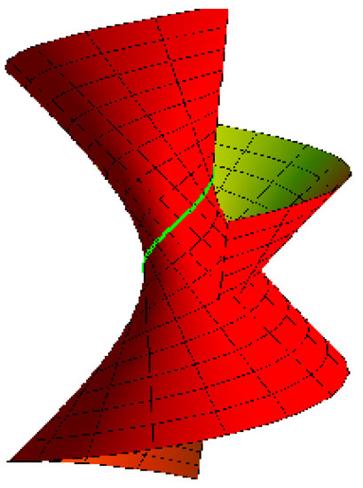Figure 1. Archimedecs helicoid.

(2)

Right helicoid with the striction curve is a helix: for $h={\psi }^{*}=1$, $\psi =\frac{\pi }{2}$, $0\le \theta \le 2\pi$ and $-3\le v\le 3$ (Figure 2),

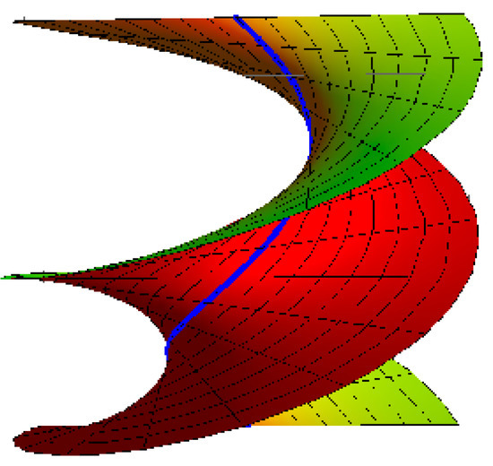Figure 2. Right helicoid.

(3)

Hyperboloid of one-sheet with the striction curve is a circle: for $h=0$, ${\psi }^{*}=1$, $\psi =\frac{\pi }{4}$, $0\le \theta \le 2\pi$ and $-7\le v\le 7$ (Figure 3),

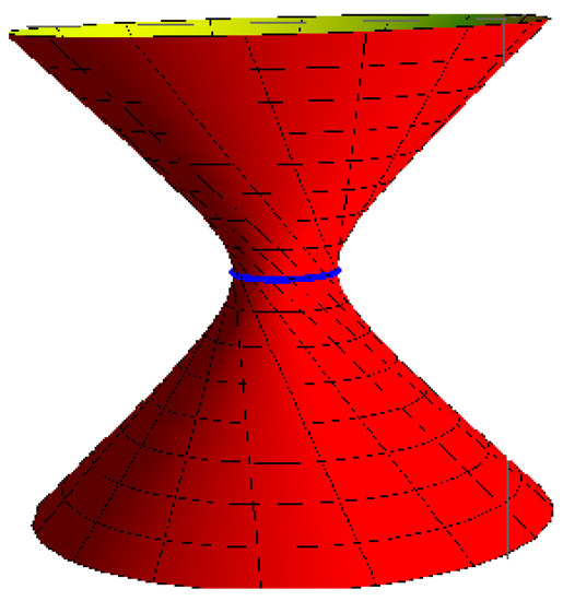Figure 3. Hyperboloid of one-sheet.

(4)

A cone with the striction curve is a point: for $h={\psi }^{*}=0$, $\psi =\frac{\pi }{4}$, $0\le \theta \le 2\pi$ and $-7\le v\le 7$ (Figure 4).

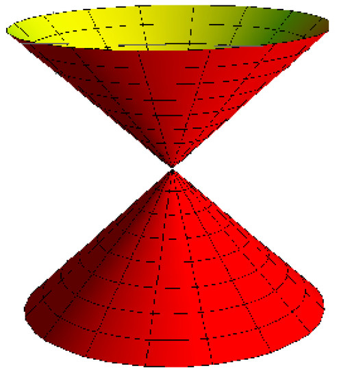Figure 4. A cone.

4. Bertrand Offsets of Ruled Surfaces

In this section, we consider the Bertrand offsets of ruled and developable surfaces, then a theory comparable to the theory of Bertrand curves can be raised for such surfaces.

Definition 1. 

Let $\left(\widehat{x}\right)$ and ($\widehat{\overline{x}}$) be two non-developable ruled surfaces in ${\mathbb{E}}^3$. The surface ($\widehat{\overline{x}}$) is said to be Bertrand offsets of $\left(\widehat{x}\right)$ if there exists a one-to-one correspondence among their rulings such that both surfaces have a mutual central normal at the corresponding striction points.

Let ($\widehat{\overline{x}}$) be a Bertrand offset of $\left(\widehat{x}\right)$ with the Blaschke frame $\{\widehat{\overline{\mathbf{x}}}\left(\widehat{\overline{s}}\right),\widehat{\overline{\mathbf{t}}}\left(\widehat{\overline{s}}\right),\widehat{\overline{\mathbf{g}}}\left(\widehat{\overline{s}}\right)\}$, it can be computed as mentioned in the above equations. Consider $\widehat{\varphi }=\varphi +\epsilon {\varphi }^{*}$ be the dual angle among the rulings of $\left(\widehat{x}\right)$ and ($\widehat{\overline{x}}$) at the corresponding points, that is,

$$<\widehat{\overline{\mathbf{x}}},\widehat{\mathbf{x}}>=cos\widehat{\varphi }.$$

(18)

By differentiating of Equation (18) with respect to $\widehat{s}$, we find

$$<\widehat{\overline{\mathbf{t}}},\widehat{\mathbf{x}}>{\widehat{\overline{s}}}^{{}^{\prime }}+<\widehat{\overline{\mathbf{x}}},\widehat{\mathbf{t}}>=-{\widehat{\varphi }}^{\prime }sin\widehat{\varphi }.$$

(19)

Since $\left(\widehat{x}\right)$ and ($\widehat{\overline{x}}$) are Bertrand offsets $(\widehat{\mathbf{t}}=\widehat{\overline{\mathbf{t}}})$, then we have ${\widehat{\varphi }}^{\prime }=0$, so that $\widehat{\varphi }=\varphi +\epsilon {\varphi }^{*}$ is an stationary dual number. Thus, the following Theorem can be given:

Theorem 2. 

The offset angle ϕ and the offset distance ${\varphi }^{*}$ among the rulings of a non-developable ruled surface and its Bertrand offset are constants.

It is evident from Theorem 2 that a ruled surface, generally, has a double infinity of Bertrand offsets. Each Bertrand offset can be formed by an stationary linear offset ${\varphi }^{*}\in \mathbb{R}$ and an stationary angular offset $\varphi \in [0,2\pi ].$ Any two surfaces of this pencil of ruled surfaces are reciprocal of one another; if ($\widehat{\overline{x}}$) is a Bertrand offset of $\left(\widehat{x}\right)$, then $\left(\widehat{x}\right)$ is likewise a Bertrand offset of ($\widehat{\overline{x}}$). So, we can write

$$\widehat{\mathbf{x}}\left(\widehat{\overline{s}}\right)=cos\widehat{\varphi }\widehat{\mathbf{x}}\left(\widehat{s}\right)+sin\widehat{\varphi }\widehat{\mathbf{g}}\left(\widehat{s}\right).$$

(20)

In the view of the fact that for a ruled surface and its Bertrand offset the central normals coincide, it follows from Theorem 1 that the central tangents of the two ruled surfaces also construct the same stationary dual angle at the matching striction points. Thus, the relationship among their Blaschke frames can be written as:

$$\left(\begin{array}{c}\widehat{\overline{\mathbf{x}}}\left(\widehat{s}\right)\hfill \\ \widehat{\overline{\mathbf{t}}}\left(\widehat{s}\right)\hfill \\ \widehat{\overline{\mathbf{g}}}\left(\widehat{s}\right)\hfill \end{array}\right)=\left(\begin{array}{ccc}cos\widehat{\varphi }\hfill & 0\hfill & sin\widehat{\varphi }\hfill \\ 0\hfill & 1\hfill & 0\hfill \\ -sin\widehat{\varphi }\hfill & 0\hfill & cos\widehat{\varphi }\hfill \end{array}\right)\left(\begin{array}{c}\widehat{\mathbf{x}}\left(\widehat{s}\right)\hfill \\ \widehat{\mathbf{t}}\left(\widehat{s}\right)\hfill \\ \widehat{\mathbf{g}}\left(\widehat{s}\right)\hfill \end{array}\right).$$

(21)

The major point to note here is the technique we have used (compared with [5,12]). The equation of the striction curve of the offset surface ($\widehat{\overline{x}}$), in terms of its base surface $\left(\widehat{x}\right)$, can therefore be written as

$$\overline{\mathbf{c}}\left(\overline{s}\right)=\mathbf{c}\left(s\right)+{\varphi }^{*}\mathbf{t}\left(s\right).$$

(22)

Hence, the equation of ($\widehat{\overline{x}}$) in terms of $\left(\widehat{x}\right)$ can be written as

$$\left(\widehat{\overline{x}}\right):\overline{\mathbf{y}}(s,v)=\mathbf{c}\left(s\right)+{\varphi }^{*}\mathbf{t}\left(s\right)+v\left(cos\varphi \mathbf{x}\left(s\right)+sin\varphi \mathbf{g}\left(s\right)\right),v\in \mathbb{R}.$$

(23)

Let $\overline{\mathsf{\xi }}(\overline{s},v)$ be the unit normal of an arbitrary point on $\left(\widehat{\overline{x}}\right)$. Then, as in Equation (6), we have:

$$\overline{\mathsf{\xi }}(\overline{s},v)=\frac{\overline{\mu }\overline{\mathbf{t}}-v\overline{\mathbf{g}}}{\sqrt{{\overline{\mu }}^2+v^2}},$$

(24)

where $\overline{\mu }$ is the distribution parameter of $\left(\widehat{\overline{x}}\right)$. It is evident from Equations (6) and (24) that the normal to a ruled surface and its Bertrand offsets are not the same. This signifies that the Bertrand offsets of a ruled surface are, generally, not parallel offsets. Therefore, the parallel conditions among ($\widehat{\overline{x}}$) in terms of $\left(\widehat{x}\right)$ can be specified by the following theorem:

Theorem 3. 

A non-developable ruled surface $\left(\widehat{x}\right)$ and its Bertrand offset ($\widehat{\overline{x}}$) are parallel offsets if and only if $\left(i\right)$ $\mu =\overline{\mu }$, $\left(ii\right)$ each edge of the Blaschke frame of $\left(\widehat{x}\right)$ is collinear with the conformable edge for ($\widehat{\overline{x}}$).

Proof. 

Suppose a non-developable ruled surface $\left(\widehat{x}\right)$ and its Bertrand offset ($\widehat{\overline{x}}$) are parallel offsets, or $\overline{\mathsf{\xi }}(\overline{s},v)\times \mathsf{\xi }(s,v)=\mathbf{0}$, we have the following expression by Equations (6) and (24)

$$v(\mu cos\varphi -\overline{\mu })\mathbf{x}+v^{2}sin\varphi \mathbf{t}+v\mu sin\varphi \mathbf{g}=\mathbf{0}.$$

The above equation should be hold true for any value $v\ne 0$, which leads to $\varphi =0$ and $\mu =\overline{\mu }$.

Suppose that the two conditions of Theorem 2 hold true, that is, $\varphi =0$, $\mu =\overline{\mu }$, and then substitute them into $\overline{\mathsf{\xi }}(\overline{s},v)\times \mathsf{\xi }(s,v)$, we have

$$\overline{\mathsf{\xi }}(\overline{s},v)\times \mathbf{n}(s,v)=\frac{\overline{\mu }\mathbf{t}-v\mathbf{g}}{\sqrt{{\overline{\mu }}^2+v^2}}\times \frac{\mu \mathbf{t}-v\mathbf{g}}{\sqrt{{\mu }^2+v^2}}$$

the result of the above equation is zero vector, which implies that $\left(\widehat{x}\right)$ and ($\widehat{\overline{x}}$) are parallel offsets. □

Deriving again in the same manner, but now for developable surface $\mu =0$, we have:

Corollary 3. 

A developable ruled surface $\left(\widehat{x}\right)$ and its developable Bertrand offset ($\widehat{\overline{x}}$) are parallel offsets if and only if each edge of the Blaschke frame of $\left(\widehat{x}\right)$ is collinear with the conformable edge for ($\widehat{\overline{x}}$).

Corollary 4. 

A developable ruled surface $\left(\widehat{x}\right)$ and its non-developable Bertrand offset ($\widehat{\overline{x}}$) can not be parallel offsets.

On the other hand, we also have

$$\frac{d}{d\widehat{\overline{s}}}\left(\begin{array}{c}\widehat{\overline{\mathbf{x}}}\left(\widehat{\overline{s}}\right)\hfill \\ \widehat{\overline{\mathbf{t}}}\left(\widehat{\overline{s}}\right)\hfill \\ \widehat{\overline{\mathbf{g}}}\left(\widehat{\overline{s}}\right)\hfill \end{array}\right)=\left(\begin{array}{ccc}0\hfill & 1\hfill & 0\hfill \\ -1\hfill & 0\hfill & \overline{\widehat{\gamma }}\hfill \\ 0\hfill & -\overline{\widehat{\gamma }}\hfill & 0\hfill \end{array}\right)\left(\begin{array}{c}\widehat{\overline{\mathbf{x}}}\left(\widehat{\overline{s}}\right)\hfill \\ \widehat{\overline{\mathbf{t}}}\left(\widehat{\overline{s}}\right)\hfill \\ \widehat{\overline{\mathbf{g}}}\left(\widehat{\overline{s}}\right)\hfill \end{array}\right),$$

(25)

where

$$d\widehat{\overline{s}}=(cos\widehat{\varphi }+\widehat{\gamma }sin\widehat{\varphi })d\widehat{s},\overline{\widehat{\gamma }}d\widehat{\overline{s}}=(\widehat{\gamma }cos\widehat{\varphi }-sin\widehat{\varphi })d\widehat{s}.$$

By eliminating $\frac{d\widehat{s}}{d\overline{\widehat{s}}}$, we attain

$$(\widehat{\overline{\gamma }}-\widehat{\gamma })cos\widehat{\varphi }+(1+\widehat{\overline{\gamma }}\widehat{\gamma })sin\widehat{\varphi }=0.$$

(26)

This is a dual version of Bertrand offsets of ruled surfaces in terms of their dual geodesic curvatures.

Theorem 4. 

The non-developable ruled surfaces $\left(\widehat{x}\right)$ and ($\widehat{\overline{x}}$) form a Bertrand offsets if and only if the Equation (23) is satisfied.

Corollary 5. 

The Bertrand offset ($\widehat{\overline{x}}$) of a helicoidal surface, generally, does not have to be a helicoidal.

Corollary 6. 

The Bertrand offset of an stationary Disteli-axis ruled surface is also an stationary Disteli-axis ruled surface.

Furthermore, the striction curve of ($\widehat{\overline{x}}$), in terms of $\mathbf{c}\left(\theta \right)$, can be written as:

$$\overline{\mathbf{c}}\left(\theta \right):=\mathbf{c}\left(\theta \right)+{\varphi }^{*}\mathbf{t}\left(\theta \right)=\left({\psi }^{*}cos\theta ,{\psi }^{*}sin\theta ,h\theta \right)+{\varphi }^{*}\left(cos\theta ,sin\theta ,0\right).$$

(27)

With the help of the Equations (17), (21) and (27), we obtain

$$\left(\widehat{\overline{x}}\right):\overline{\mathbf{y}}(\theta ,v)=\left(\begin{array}{c}({\psi }^{*}+{\varphi }^{*})cos\theta +vsin(\psi -\varphi )sin\theta \\ ({\psi }^{*}+{\varphi }^{*})sin\theta -vsin(\psi -\varphi )cos\theta \\ h\theta +vcos(\psi -\varphi )\end{array}\right).$$

(28)

Example 1. 

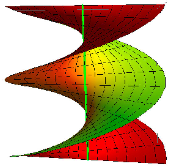
In this example, we verify the idea of Corollary 5. In view of Theorem 1, and Equation (26) we have that: $\widehat{\gamma }=cot\widehat{\psi }=0$ ($\psi =\frac{\pi }{2}$, ${\psi }^{*}=0$)$\iff \widehat{\overline{\gamma }}+cot\widehat{\varphi }=0$. Then, in view of Equations (17) and (28), the ruled surface

$$\left(\widehat{\overline{x}}\right):\overline{\mathbf{y}}(\theta ,v)=\left(\begin{array}{c}{\varphi }^{*}cos\theta +vcos\varphi sin\theta \\ {\varphi }^{*}sin\theta -vcos\varphi cos\theta \\ h\theta +vsin\varphi \end{array}\right),$$

is the Bertrand offset of the helicoidal surface (Figure 5)

$$\left(\widehat{x}\right):\mathbf{y}(\theta ,v)=(vsin\theta ,-vcos\theta ,h\theta ).$$

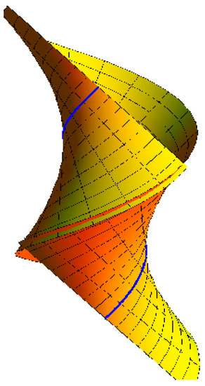
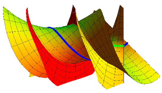
Take ${\varphi }^{*}=1$, $\varphi =\frac{\pi }{4}$ and$h=1$ for example the Bertrand offset is shown Figure 6; where $0\le \theta \le 2\pi ,$ $-3\le v\le 3$. The graph of the helicoidal surface $\left(\widehat{x}\right)$ with its Bertrand offset $\left(\widehat{\overline{x}}\right)$ is shown in Figure 7.

Figure 5. Helicoidal surface.

Figure 6. Bertrand offset of the helicoidal surface.

Figure 7. Helicoidal surface with its Bertrand offset.

The Striction Curves

In this subsection, we consider the striction curves of the Bertrand offsets. With the aid of Equation (19), the tangent of the striction curve $\overline{\mathbf{c}}\left(\overline{s}\right)$ of ($\widehat{\overline{x}}$) is

$$\frac{d\overline{\mathbf{c}}\left(\overline{s}\right)}{d\overline{s}}=\left[(\mathit{𝘍}-{\varphi }^{*})\mathbf{x}+(\mu +\gamma {\varphi }^{*})\mathbf{g}\right]\frac{ds}{d\overline{s}},$$

(29)

whereas, as in Equation (4), is:

$$\frac{d\overline{\mathbf{c}}\left(\overline{s}\right)}{d\overline{s}}=\overline{\mathit{𝘍}}\left(\overline{s}\right)\overline{\mathbf{x}}\left(\overline{s}\right)+\overline{\mu }\left(\overline{s}\right)\overline{\mathbf{g}}\left(\overline{s}\right).$$

(30)

From Equations (29) and (30) we attain

$$\frac{d\overline{s}}{ds}=\frac{\mathit{𝘍}-{\varphi }^{*}}{\overline{\mathit{𝘍}}cos\varphi +\overline{\mu }sin\varphi }=\frac{\mu +\gamma {\varphi }^{*}}{-\overline{\mathit{𝘍}}sin\varphi +\overline{\mu }cos\varphi }.$$

(31)

Hence, we have two main different cases:

(a) In the case of ($\widehat{x}$) is tangential surface, that is, $\mu =0$. In this case the Blaschke frame $\left\{\mathbf{x}\right(s),$ $\mathbf{t}\left(s\right)$, $\mathbf{g}\left(s\right)\}$ turn into the classical Serret-Frenet frame $\left\{\mathbf{t}\right(s),$ $\mathbf{n}\left(s\right)$, $\mathbf{b}\left(s\right)\}$ and the striction curve $\mathbf{c}\left(s\right)$ turns out to be the edge of regression of ($\widehat{x}$). Therefore, we find

$$\left(\begin{array}{c}\overline{\mathbf{t}}\hfill \\ \overline{\mathbf{n}}\hfill \\ \overline{\mathbf{b}}\hfill \end{array}\right)=\left(\begin{array}{ccc}cos\varphi \hfill & 0\hfill & -sin\varphi \hfill \\ 0\hfill & 1\hfill & 0\hfill \\ sin\varphi \hfill & 0\hfill & cos\varphi \hfill \end{array}\right)\left(\begin{array}{c}\mathbf{t}\hfill \\ \mathbf{n}\hfill \\ \mathbf{b}\hfill \end{array}\right),$$

(32)

and

$$\overline{\mathbf{c}}\left(\overline{s}\right)=\mathbf{c}\left(s\right)+{\varphi }^{*}\mathbf{n}\left(s\right).$$

(33)

Moreover, the curvature $\kappa \left(s\right)$ and the torsion $\tau \left(s\right)$ of $\mathbf{c}\left(s\right)$ can be specified by

$$\kappa \left(s\right)=\frac{1}{\mathit{𝘍}\left(s\right)},\tau \left(s\right)=\frac{\gamma \left(s\right)}{\mathit{𝘍}\left(s\right)}.$$

Therefore, from Equation (31) we have

$$\overline{\mu }=\overline{\mathit{𝘍}}\frac{\left(1-{\varphi }^{*}\kappa \right)sin\varphi +\tau {\varphi }^{*}cos\varphi }{\left(1-{\varphi }^{*}\kappa \right)cos\varphi -\tau {\varphi }^{*}sin\varphi }.$$

(34)

Thus the Bertrand offset of a developable surface is not developable, that is, $\overline{\mu }\left(s\right)\ne 0$. Furthermore, if the ruled surface ($\widehat{\overline{x}}$) is also a tangential developable, that is, $\overline{\mu }\left(s\right)=0$. Then, from Equation (34), we gain

$$\left(1-{\varphi }^{*}\kappa \right)sin\varphi +\tau {\varphi }^{*}cos\varphi =0.$$

(35)

Theorem 5. 

$\left(\widehat{x}\right)$ and ($\widehat{\overline{x}}$) are tangential Bertrand offsets if and only if their striction curves are Bertrand curves.

Corollary 7. 

(i)

If $\varphi =0$, then ${\varphi }^{*}=0$ or $\tau =0$,

(ii)

If ${\varphi }^{*}=0$, then $\varphi =0$, that is, the rulings are identical,

(iii)

If $\tau =0$, and ${\varphi }^{*}\ne 0$, then $\kappa \left(\upsilon \right)=1/{\varphi }^{*}$ is stationary or $\varphi =0$,

(iv)

$\varphi =\pi /2$, and ${\varphi }^{*}\ne 0,$ then $\kappa \left(\upsilon \right)=1/{\varphi }^{*}$ is stationary.

From Equation (28), we also have

$$cos\varphi d\overline{s}=(1-{\varphi }^{*}\kappa )ds,\mathrm{and}sin\varphi d\overline{s}+{\varphi }^{*}\tau ds=0.$$

(36)

If $\mathbf{c}\left(s\right)=\mathbf{c}(s+2\pi )$ ($\overline{\mathbf{c}}\left(\overline{s}\right)=\overline{\mathbf{c}}(\overline{s}+2\pi )$), then ($\widehat{x}$) (resp. (x)) is a closed tangential surface. Let $\mathcal{L}$ (resp. $\overline{\mathcal{L}}$) be the length of the edge of regression of ($\widehat{x}$) (resp. ($\widehat{\overline{x}}$)) $\mathbf{c}\left(\upsilon \right)$. Since both ${\varphi }^{*}$, and $\varphi$ are stationary, integration of the first expression in Equation (36) yields

$$\overline{\mathcal{L}}cos\varphi =\mathcal{L}-{\varphi }^{*}\underset{\mathbf{c}\left(s\right)}{\oint }\kappa ds.$$

If $\overline{\mathbf{n}}=-\mathbf{n}$, then $\mathbf{c}\left(s\right)=\overline{\mathbf{c}}\left(\overline{s}\right)+{\varphi }^{*}\overline{\mathbf{n}}\left(\overline{s}\right)$, so by the symmetry of the mating relationship,

$$\mathcal{L}cos\overline{\varphi }=\overline{\mathcal{L}}-{\varphi }^{*}\underset{\overline{\mathbf{c}}\left(\overline{s}\right)}{\oint }\overline{\kappa }d\overline{s}.$$

Hence $cos\varphi =cos\overline{\varphi }$, and adding the previous two equations

$$\left(\overline{\mathcal{L}}+\mathcal{L}\right)(1-cos\varphi )={\varphi }^{*}\left(\underset{\mathbf{c}\left(s\right)}{\oint }\kappa ds+\underset{\overline{\mathbf{c}}\left(\overline{s}\right)}{\oint }\overline{\kappa }d\overline{s}\right),$$

(37)

or

$$\left(\overline{\mathcal{L}}+\mathcal{L}\right){sin}^2\frac{\varphi }{2}=\frac{{\varphi }^{*}}{2}\left(\underset{\mathbf{c}\left(s\right)}{\oint }\kappa ds+\underset{\overline{\mathbf{c}}\left(\overline{s}\right)}{\oint }\overline{\kappa }d\overline{s}\right).$$

(38)

In view of the Fenchel’s inequality [17], we have

$$\overline{\mathcal{L}}+\mathcal{L}\ge 2\pi {\varphi }^{*}.$$

Corollary 8. 

The sum of the lengths of the striction curves of the tangential offsets is never inferior to $2\pi$ times the distance through their corresponding points.

If the striction curve $\mathbf{c}\left(s\right)$ is self-mated curve, that is, $\overline{\mathbf{c}}\left(s\right)=\mathbf{c}\left(s\right)$, the Formula (37) turn into

$$\mathcal{L}=\frac{{\varphi }^{*}}{1-cos\varphi }\underset{\mathbf{c}\left(s\right)}{\oint }\kappa \left(s\right)ds,\mathrm{with}1-cos\varphi \ne 0.$$

(39)

If $\varphi =(2p+1)\pi$ (p is an integer) then $cos\varphi =-1$, and therefore Equation (39) become

$$\mathcal{L}=\frac{{\varphi }^{*}}{2}\underset{\mathbf{c}\left(s\right)}{\oint }\kappa \left(s\right)ds.$$

(40)

Furthermore, if the striction curve $\mathbf{c}\left(s\right)$ is a planar curve, then

$$\underset{\mathbf{c}\left(s\right)}{\oint }\kappa \left(s\right)ds=2\pi .$$

(41)

From Equations (40) and (41) we get $\mathcal{L}=\pi {\varphi }^{*}$. Thus we have the following theorem:

Theorem 6. 

The length of a self-mated striction curve $\mathbf{c}\left(s\right)$ of ($\widehat{x}$) is π times its width (breadth).

(b) In the case of ($\widehat{x}$) is a binormal surface, that is, $\mathit{𝘍}=0$. In this case, from Equation (31), we have:

$$\overline{\mathit{𝘍}}=\overline{\mu }\frac{{\varphi }^{*}cos\varphi -\left(\gamma {\varphi }^{*}+\mu \right)sin\varphi }{{\varphi }^{*}sin\varphi +\left(\gamma {\varphi }^{*}+\mu \right)cos\varphi }.$$

(42)

Thus the Bertrand offset of a binormal is not binormal, that is, $\overline{\mathit{𝘍}}\left(s\right)\ne 0$. Further, if the Bertrand offset ($\widehat{\overline{x}}$) is also a binormal, then we can find:

$$(1+{\varphi }^{*}\kappa )sin\varphi -{\varphi }^{*}\tau cos\varphi =0.$$

Theorem 7. 

$\left(\widehat{x}\right)$ and ($\widehat{\overline{x}}$) are binormal Bertrand offsets if and only if their striction curves are Bertrand curves.

In a similar manner, all the results of the tangential surface may be given for the binormal ruled surface.

5. Conclusions

In this study, an extension of Bertrand offsets of curves for ruled, and developable surfaces has been improved. Noteworthy, there are numerous similarities through the Bertrand curves and the Bertrand offsets for ruled surfaces. For example, a ruled surface can have an infinity of Bertrand offsets in analogy with a plane curve can have an infinity of Bertrand mates. From this result the proofs of the theorems of Fenchel and Barbier are reproved by an elegant method. Meanwhile, the derivations of some useful geometric relations, examples and instructive figures of the ruled surfaces are included. For future study, we will catch with the novel ideas that Gaussian and mean curvatures of these Bertrand offsets can be gained, when the Weingarten map for the Bertrand offsets ruled surfaces is realized. We will also address integrating the work of singularity theory and submanifold theory and so forth, given in [19,20,21,22], with the results of this paper to explore new methods to find more theorems related to symmetric properties on this subject.

References

- Veldkamp, G.R. On the use of Dual numbers, Vectors, and Matrices in Instantaneous Spatial Kinematics. Mech. Mach. Theory 1976, 11, 141–156. [Google Scholar] [CrossRef]
- Bottema, O.; Roth, B. Theoretical Kinematics; North-Holland Press: New York, NY, USA, 1979. [Google Scholar]
- Karger, A.; Novak, J. Space Kinematics and Lie Groups; Gordon and Breach Science Publishers: New York, NY, USA, 1985. [Google Scholar]
- Pottman, H.; Wallner, J. Computational Line Geometry; Springer: Berlin/Heidelberg, Germany, 2001. [Google Scholar]
- Ravani, B.; Ku, T.S. Bertrand offsets of ruled and developable surfaces. Comput. Aided Des. 1991, 23, 145–152. [Google Scholar] [CrossRef]
- Küçük, A.; Gürsoy, O. On the invariants of Bertrand trajectory surface offsets. AMC 2003, 11–23. [Google Scholar] [CrossRef]
- Kasap, E.; Kuruoglu, N. Integral invariants of the pairs of the Bertrand ruled surface. Bull. Pure Appl. Sci. Sect. E Math. 2002, 21, 37–44. [Google Scholar]
- Kasap, E.; Kuruoglu, N. The Bertrand offsets of ruled surfaces in . Acta Math Vietnam 2006, 31, 39–48. [Google Scholar]
- Kasap, E.; Yuce, S.; Kuruoglu, N. The involute-evolute offsets of ruled surfaces. Iran. Sci Tech Trans. A 2009, 33, 195–201. [Google Scholar]
- Orbay, K.; Kasap, E.; Aydemir, I. Mannheim offsets of ruled surfaces. Math. Probl. Eng. 2009, 2009, 160917. [Google Scholar] [CrossRef]
- Onder, M.; Ugurlu, H.H. Frenet frames and invariants of timelike ruled surfaces. Ain. Shams Eng. J. 2013, 4, 507–513. [Google Scholar] [CrossRef]
- Aldossary, M.T.; Abdel-Baky, R.A. On the Bertrand offsets for ruled and developable surfaces. Boll. Unione Mat. Ital. 2015, 8, 53–64. [Google Scholar] [CrossRef]
- Sentrk, G.Y.; Yuce, S. Properties of integral invariants of the involute-evolute offsets of ruled surfaces. Int. J. Pure Appl. Math. 2015, 102, 75. [Google Scholar] [CrossRef]
- Sentrk, G.Y.; Yuce, S.; Kasap, E. Integral Invariants of Mannheim offsets of ruled surfaces. Appl. Math. E-Notes 2016, 16, 198–209. [Google Scholar]
- Sentrk, G.Y.; Yuce, S. Bertrand offsets of ruled surfaces with Darboux frame. Results Math. 2017, 72, 1151–1159. [Google Scholar] [CrossRef]
- Sentrk, G.Y.; Yuce, S. On the evolute offsets of ruled surfaces usin the Darboux frame. Commun. Fac. Sci. Univ. Ank. Ser. A1 Math. Stat. Vo. 2019, 68, 1256–1264. [Google Scholar] [CrossRef]
- Gugenheimer, H.W. Differential Geometry; Graw-Hill: New York, NY, USA, 1956. [Google Scholar]
- Bruce, J.W.; Giblin, P.J. Curves and Singularities, 2nd ed.; Cambridge University Press: Cambridge, UK, 1992. [Google Scholar]
- Li, Y.L.; Zhu, Y.S.; Sun, Q.Y. Singularities and dualities of pedal curves in pseudo-hyperbolic and de Sitter space. Int. J. Geom. Methods Mod. Phys. 2021, 18, 1–31. [Google Scholar] [CrossRef]
- Li, Y.L.; Nazra, S.; Abdel-Baky, R.A. Singularities Properties of timelike sweeping surface in Minkowski 3-Space. Symmetry 2022, 14, 1996. [Google Scholar] [CrossRef]
- Li, Y.L.; Chen, Z.; Nazra, S.; Abdel-Baky, R.A. Singularities for timelike developable surfaces in Minkowski 3-Space. Symmetry 2023, 15, 277. [Google Scholar] [CrossRef]
- Almoneef, A.A.; Abdel-Baky, R.A. Singularity properties of spacelike circular surfaces. Symmetry 2023, 15, 842. [Google Scholar] [CrossRef]
Disclaimer/Publisher’s Note: The statements, opinions and data contained in all publications are solely those of the individual author(s) and contributor(s) and not of MDPI and/or the editor(s). MDPI and/or the editor(s) disclaim responsibility for any injury to people or property resulting from any ideas, methods, instructions or products referred to in the content. |
© 2023 by the authors. Licensee MDPI, Basel, Switzerland. This article is an open access article distributed under the terms and conditions of the Creative Commons Attribution (CC BY) license (https://creativecommons.org/licenses/by/4.0/).