Some New Bullen-Type Inequalities Obtained via Fractional Integral Operators

Abstract

In this paper, we establish a new auxiliary identity of the Bullen type for twice-differentiable functions in terms of fractional integral operators. Based on this new identity, some generalized Bullen-type inequalities are obtained by employing convexity properties. Concrete examples are given to illustrate the results, and the correctness is confirmed by graphical analysis. An analysis is provided on the estimations of bounds. According to calculations, improved Hölder and power mean inequalities give better upper-bound results than classical inequalities. Lastly, some applications to quadrature rules, modified Bessel functions and digamma functions are provided as well.

1. Introduction

Convexity (concavity) has many applications in several fields, which include mathematics, economics, finance, engineering and computer science. Numerous noteworthy inequalities and properties can be found in various categories of mathematics employing convexity (concavity) theory (see [1,2,3,4]). The unique global minimum in convex optimization problems can be efficiently located by applying a variety of optimization methods, including gradient descent, Newton’s method and interior-point approaches. In applied problems, especially in optimization problems, the role of the concept of convexity is well-known. This concept, along with the functions derived from it, has a special place in the theory of integral inequalities; for example the inequalities of Jensen, Hermite, Simpson, Bullen, etc. (see [5,6,7]). Here, we first recall some necessary definitions and inequalities (see [8] and references therein).

Definition 1. 

The function $\psi :\left[\vartheta {}^{\ast },\varrho {}^{\ast }\right]\to \mathbb{R}$ is said to be convex if we have

$$\psi \left(\epsilon \rho +\left(1-\epsilon \right)y\right)\le \epsilon \psi \left(\rho \right)+\left(1-\epsilon \right)\psi \left(y\right),$$

for all $\rho ,y\in \left[\vartheta {}^{\ast },\varrho {}^{\ast }\right]$ and $\epsilon \in \left[0,1\right].$ If $-\psi$ is convex, then ψ is concave.

The double Hermite–Hadamard inequality (hereinafter the Hadamard inequality), widely known in the theory of inequalities, is closely related to convex functions. This inequality is formulated in the literature as follows:

Let $\psi$:$\left[\vartheta {}^{\ast },\varrho {}^{\ast }\right]\to \mathbb{R}$ be a convex function. Then, we have the following double inequality:

$$\psi \left(\frac{\vartheta {}^{\ast }+\varrho {}^{\ast }}{2}\right)\le \frac{1}{\varrho {}^{\ast }-\vartheta {}^{\ast }}{\int }_{\vartheta {}^{\ast }}^{\varrho {}^{\ast }}\psi \left(\epsilon \right)d\epsilon \le \frac{\psi \left(\vartheta {}^{\ast }\right)+\psi \left(\varrho {}^{\ast }\right)}{2}.$$

(1)

Many important inequalities have been established in the literature for various classes of convex functions and classes derived from them (for example, see [2,9,10,11]).

In [12], Bullen proved the following inequality, which is known as Bullen’s inequality, for the convex function $\psi$:

$$\frac{1}{\varrho {}^{\ast }-\vartheta {}^{\ast }}{\int }_{\vartheta {}^{\ast }}^{\varrho {}^{\ast }}\psi \left(\epsilon \right)d\epsilon \le \frac{1}{2}\left[\psi \left(\frac{\vartheta {}^{\ast }+\varrho {}^{\ast }}{2}\right)+\frac{\psi \left(\vartheta {}^{\ast }\right)+\psi \left(\varrho {}^{\ast }\right)}{2}\right].$$

(2)

The well-known Bullen’s inequality was first presented by Bullen in 1978 [12]. Due to their outstanding uses, Bullen-type inequalities have garnered a lot of interest. Bullen’s inequality is a topic that many scientists and mathematicians are very interested in and concerned about because of its importance in many different domains. Bullen’s inequality has drawn a lot of interest from scholars, who have worked hard over the years to enhance and generalize it. Numerous researchers have generalized the well-known Bullen’s inequality in its conventional form for various subcategories of convex functions. Recently, there have been many interesting and attention-grabbing studies in the literature devoted to improving and generalizing Bullen-type inequalities. For example, some of these works are listed below.

In [13], Cakmak established some inequalities of the Hadmard and Bullen types for Lipschitzian functions. In [14], Çakmak presented Bullen-type inequalities via fractional integral operators for differentiable convex and $h—$convex functions and gave good examples. In [15] (see also [16]), Erden and Sarikaya established generalized Bullen-type inequalities using local fractional integrals and some applications for special means were given. In [17], Işcan et al. obtained some generalized Hadamard- and Bullen-type inequalities for convex functions and described some applications and error estimates for the left and right Hadamard inequalities. In [18], Hussain and Mehboob, using the generalized fractional integral identity, derived new estimates for the Bullen-type functional for $(s,p)—$convex functions. In [19], Yaşar et al. presented the Bullen-, midpoint-, trapezoid- and Simpson-type inequalities for s-convex functions in the fourth sense. In [20], Boulares et al. presented fractional multiplicative Bullen-type inequalities, along with some applications, using multiplicative calculus. Recently, in [21], Bahtiyar et al. gave a uniform treatment of fractional Bullen-type inequalities to provide a concrete estimation analysis of bounds using Lipschitz functions, mean value theorem and convexity theory.

It was inevitable that fractional calculus would arise using arbitrary-order integrals and derivatives. Due to its applicability in numerous fields of science and engineering, this topic has gained considerable prominence. The fact that researchers have over time suggested more efficient solutions to physical phenomena attuned to new operators with dominant kernels is a significant difference in this subject. Fractional derivatives play an important role in a number of mathematical problems and the corresponding practical consequences [22,23]. The fractional calculus approach has recently been employed to define the intricate dynamics of problems in real-life scenarios in several branches of applied science domains. There are numerous uses in the literature [24,25]. Fractional calculus has been widely employed to achieve novel results in the theory of inequality, connecting fractional operators through the idea of convexity (see [26,27,28,29,30]). We need the following definition of classical integral operators:

Definition 2 

([23]). Let $\psi \in L\left[\vartheta {}^{\ast },\varrho {}^{\ast }\right].$ The Riemann–Liouville integrals $J_{\vartheta {{}^{\ast }}^{+}}^{\alpha }\psi$ and $J_{{{\varrho }^{\ast }}^{-}}^{\alpha }\psi$ of order $\alpha >0$ with $\vartheta {}^{\ast }\ge 0$ are defined by

$$J_{\vartheta {{}^{\ast }}^{+}}^{\alpha }\psi \left(\rho \right)=\frac{1}{\Gamma \left(\alpha \right)}{\int }_{\vartheta {}^{\ast }}^{\rho }{\left(\rho -\epsilon \right)}^{\alpha -1}\psi \left(\epsilon \right)d\epsilon ,\rho >\vartheta {}^{\ast }$$

and

$$J_{\varrho {}^{\ast }-}^{\alpha }\psi \left(\rho \right)=\frac{1}{\Gamma \left(\alpha \right)}{\int }_{\rho }^{\varrho {}^{\ast }}{\left(\epsilon -\rho \right)}^{\alpha -1}\psi \left(\epsilon \right)d\epsilon ,\rho <\varrho {}^{\ast },$$

respectively, where $\Gamma \left(\alpha \right)={\int }_0^{\infty }{e}^{-u}{u}^{\alpha -1}du.$ Here we have $J_{a^{+}}^0\psi \left(x\right)=J_{b^{-}}^0\psi \left(\rho \right)=\psi \left(\rho \right).$ In the case of $\alpha =1$, the fractional integral reduces to the classical integral.

Two classical inequalities—namely, the Hölder inequality and its other form—and the power mean inequalities have been used frequently in the development of the theory of integral inequalities.

Theorem 1 

(Hölder inequality). Let $p>1$, $\frac{1}{p}+\frac{1}{q}=1$ and $\psi \left(\epsilon \right)$,$g\left(\epsilon \right):[\vartheta {}^{\ast },\varrho {}^{\ast }]⟶\mathbb{R}$. If ${|\psi |}^p,{|g|}^q$$\in L[\vartheta {}^{\ast },\varrho {}^{\ast }]$, then

$${\int }_{\vartheta {}^{\ast }}^{\varrho {}^{\ast }}\left|\psi \left(\epsilon \right)g\left(\epsilon \right)\right|d\epsilon \le {\left({\int }_{\vartheta {}^{\ast }}^{\varrho {}^{\ast }}{\left|\psi \left(\epsilon \right)\right|}^{p}d\epsilon \right)}^{\frac{1}{p}}{\left({\int }_{\vartheta {}^{\ast }}^{\varrho {}^{\ast }}{\left|g\left(\epsilon \right)\right|}^{q}d\epsilon \right)}^{\frac{1}{q}},$$

(3)

for which equality holds if and only if ${A|\psi \left(\epsilon \right)|}^p$$={B|g\left(\epsilon \right)|}^q$ almost everywhere, where A and B are constants.

Theorem 2 

(Improved Hölder integral inequality [31]). Let $p>1,$$\frac{1}{p}+\frac{1}{q}=1$ and $\psi \left(\epsilon \right)$,$g\left(\epsilon \right)$:$[\vartheta {}^{\ast },\varrho {}^{\ast }]⟶\mathbb{R}$. If ${|\psi |}^p$, ${|g|}^q$$\in L[\vartheta {}^{\ast },\varrho {}^{\ast }],$ then

$$\begin{array}{cc}\hfill & {\int }_{\vartheta {}^{\ast }}^{\varrho {}^{\ast }}\left|\psi \left(\epsilon \right)g\left(\epsilon \right)\right|d\epsilon \hfill \\ \hfill & \le \frac{1}{\varrho {}^{\ast }-\vartheta {}^{\ast }}{\left({\int }_{\vartheta {}^{\ast }}^{\varrho {}^{\ast }}(\varrho {}^{\ast }-\epsilon ){|\psi \left(\epsilon \right)|}^{p}d\epsilon \right)}^{\frac{1}{p}}{\left({\int }_{\vartheta {}^{\ast }}^{\varrho {}^{\ast }}(\varrho {}^{\ast }-\epsilon ){|g\left(\epsilon \right)|}^{q}d\epsilon \right)}^{\frac{1}{q}}\hfill \\ \hfill & +\frac{1}{\varrho {}^{\ast }-\vartheta {}^{\ast }}{\left({\int }_{\vartheta {}^{\ast }}^{{\varrho }^{\ast }}(\epsilon -\vartheta {}^{\ast }){|\psi \left(\epsilon \right)|}^{p}d\epsilon \right)}^{\frac{1}{p}}{\left({\int }_{\vartheta {}^{\ast }}^{\varrho {}^{\ast }}(\epsilon -\vartheta {}^{\ast }){|g\left(\epsilon \right)|}^{q}d\epsilon \right)}^{\frac{1}{q}}.\hfill \end{array}$$

(4)

Theorem 3 

(Power mean inequality). Let $q\ge 1,$$\frac{1}{p}+\frac{1}{q}=1$ and $\psi \left(\epsilon \right)$,$g\left(\epsilon \right):[\vartheta {}^{\ast },\varrho {}^{\ast }]⟶\mathbb{R}$. If ${|\psi |}^p,{|g|}^q$$\in L[\vartheta {}^{\ast },\varrho {}^{\ast }]$, then

$${\int }_{\vartheta {}^{\ast }}^{\varrho {}^{\ast }}\left|\psi \left(\epsilon \right)g\left(\epsilon \right)\right|d\epsilon \le {\left({\int }_{\vartheta {}^{\ast }}^{\varrho {}^{\ast }}\left|\psi \left(\epsilon \right)\right|d\epsilon \right)}^{1-\frac{1}{q}}{\left({\int }_{\vartheta {}^{\ast }}^{\varrho {}^{\ast }}\left|\psi \left(\epsilon \right)\right|{\left|g\left(\epsilon \right)\right|}^{q}d\epsilon \right)}^{\frac{1}{q}}.$$

(5)

Theorem 4 

(Improved power mean integral inequality [32]). Let $q\ge 1$ and $\psi \left(\epsilon \right)$, $g\left(\epsilon \right)$:$[\vartheta {}^{\ast },\varrho {}^{\ast }]$$⟶\mathbb{R}$. If ${|\psi |,|g|}^q$$\in L[\vartheta {}^{\ast },\varrho {}^{\ast }]$ are the integrable functions on $[\vartheta {}^{\ast },\varrho {}^{\ast }]$, then

$$\begin{array}{cc}\hfill & {\int }_{\vartheta {}^{\ast }}^{\varrho {}^{\ast }}|\psi \left(\epsilon \right)g\left(\epsilon \right)|d\epsilon \hfill \\ \hfill & \le \frac{1}{\varrho {}^{\ast }-\vartheta {}^{\ast }}{\left({\int }_{\vartheta {}^{\ast }}^{\varrho {}^{\ast }}(\varrho {}^{\ast }-\epsilon )|\psi \left(\epsilon \right)|d\epsilon \right)}^{1-\frac{1}{q}}{\left({\int }_{\vartheta {}^{\ast }}^{\varrho {}^{\ast }}(\varrho {}^{\ast }-\epsilon )|\psi \left(\epsilon \right)||g\left(\epsilon \right){|}^{q}d\epsilon \right)}^{\frac{1}{q}}\hfill \\ \hfill & +\frac{1}{\varrho {}^{\ast }-\vartheta {}^{\ast }}{\left({\int }_{\vartheta {}^{\ast }}^{\varrho {}^{\ast }}(\epsilon -\vartheta {}^{\ast })|\psi \left(\epsilon \right)|d\epsilon \right)}^{1-\frac{1}{q}}{\left({\int }_{\vartheta {}^{\ast }}^{\varrho {}^{\ast }}(\epsilon -\vartheta {}^{\ast })|\psi \left(\epsilon \right)||g\left(\epsilon \right){|}^{q}d\epsilon \right)}^{\frac{1}{q}}.\hfill \end{array}$$

(6)

In [33], U. Kırmacı proved the following lemma.

Lemma 1. 

Let $\psi :\left[\vartheta {}^{\ast },\varrho {}^{\ast }\right]\to \mathbb{R}$ and $\psi \in$$C^2\left(\vartheta {}^{\ast },\varrho {}^{\ast }\right)$ with ${\psi }^{″}\in L[\vartheta {}^{\ast },\varrho {}^{\ast }].$ Then, we have

$$\frac{{(\varrho {}^{\ast }-\vartheta {}^{\ast })}^2}{2}(I_1+I_2)=\frac{1}{\varrho {}^{\ast }-\vartheta {}^{\ast }}{\int }_{\vartheta {}^{\ast }}^{\varrho {}^{\ast }}\psi \left(\epsilon \right)d\epsilon -\frac{1}{2}\left[\frac{\psi \left(\vartheta {}^{\ast }\right)+\psi \left(\varrho {}^{\ast }\right)}{2}+\psi \left(\frac{\vartheta {}^{\ast }+\varrho {}^{\ast }}{2}\right)\right],$$

(7)

where

$$\begin{array}{ccc}\hfill I_1& =& {\int }_0^{1/2}\epsilon \left(\epsilon -0.5\right){\psi }^{″}(\vartheta {}^{\ast }\epsilon +\varrho {}^{\ast }(1-\epsilon ))d\epsilon ,\hfill \\ \hfill I_2& =& {\int }_{1/2}^1\left(\epsilon -0.5\right)\left(\epsilon -1\right){\psi }^{″}(\vartheta {}^{\ast }\epsilon +\varrho {}^{\ast }(1-\epsilon ))d\epsilon .\hfill \end{array}$$

The main objective of this paper is to obtain some generalized Bullen-type inequalities for continuously differentiable functions. We first establish an identity of the Bullen type for twice-differentiable functions in terms of fractional integral operators. Based on this new identity, some generalized Bullen-type inequalities are obtained by employing convexity properties. Concrete examples are constructed to illustrate the results, and the correctness is verified by graphical analysis. An analysis is provided on the estimations of bounds. According to calculations, improved Hölder and power mean inequalities give better upper-bound results than classical inequalities. Lastly, some applications to quadrature rules, modified Bessel functions and digamma functions are provided as well.

2. Main Results

We start the results in this section by proving the following lemma.

Lemma 2. 

Let ψ:$\left[\vartheta {}^{\ast },\varrho {}^{\ast }\right]\to \mathbb{R}$ and $\psi \in$$C^2\left(\vartheta {}^{\ast },\varrho {}^{\ast }\right)$ with ${\psi }^{″}\in L[\vartheta {}^{\ast },\varrho {}^{\ast }]$. When $\forall \varkappa \in [0,1]$, the equality holds:

$$\begin{array}{cc}\hfill & \psi \left(c\right)-\mathbf{F}\left\{\frac{\alpha +1}{\varrho {}^{\ast }-\vartheta {}^{\ast }}\left[J_{c^{+}}^{\alpha }\psi \left(\varrho {}^{\ast }\right)+J_{c^{-}}^{\alpha }\psi \left(\vartheta {}^{\ast }\right)\right]-\left[\varkappa J_{c^{+}}^{\alpha -1}\psi \left(\varrho {}^{\ast }\right)+(1-\varkappa )J_{c^{-}}^{\alpha -1}\psi \left(\vartheta {}^{\ast }\right)\right]\right\}\hfill \\ \hfill & =\frac{{\left(\varrho {}^{\ast }-\vartheta {}^{\ast }\right)}^2}{{\varkappa }^{\alpha }+{(1-\varkappa )}^{\alpha }}\left(I_1+I_2\right),\hfill \end{array}$$

(8)

where $c=\varkappa \vartheta {}^{\ast }+(1-\varkappa )\varrho {}^{\ast },\alpha >1$, $\mathbf{F}=\frac{\Gamma (\alpha +1)}{\left[{\varkappa }^{\alpha }+{(1-\varkappa )}^{\alpha }\right]{\left(\varrho {}^{\ast }-\vartheta {}^{\ast }\right)}^{\alpha -1}},$

$$\begin{array}{cc}\hfill I_1& ={\int }_0^{\varkappa }{\epsilon }^{\alpha }\left(\varkappa -\epsilon \right){\psi }^{″}(\vartheta {}^{\ast }\epsilon +\varrho {}^{\ast }(1-\epsilon ))d\epsilon ,\hfill \\ \hfill I_2& ={\int }_{\varkappa }^1\left(\epsilon -\varkappa \right){\left(1-\epsilon \right)}^{\alpha }{\psi }^{″}(\vartheta {}^{\ast }\epsilon +\varrho {}^{\ast }(1-\epsilon ))d\epsilon .\hfill \end{array}$$

Proof. 

By integrating the first integral by parts twice, we get

$$\begin{array}{cc}\hfill I_1& =-\frac{1}{\vartheta {}^{\ast }-\varrho {}^{\ast }}{\int }_0^{\varkappa }\left[\varkappa \alpha {\epsilon }^{\alpha -1}-\left(\alpha +1\right){\epsilon }^{\alpha }\right]{\psi }^{\prime }(\vartheta {}^{\ast }\epsilon +\varrho {}^{\ast }(1-\epsilon ))d\epsilon \hfill \\ \hfill & =-\frac{1}{\vartheta {}^{\ast }-\varrho {}^{\ast }}\left[\frac{\varkappa \alpha {\epsilon }^{\alpha -1}-\left(\alpha +1\right){\epsilon }^{\alpha }}{\vartheta {}^{\ast }-\varrho {}^{\ast }}\psi (\epsilon \vartheta {}^{\ast }+(1-\epsilon ){\varrho }^{\ast }){|}_0^{\varkappa }\right.\hfill \\ \hfill & \left.-\frac{1}{\vartheta {}^{\ast }-\varrho {}^{\ast }}{\int }_0^{\varkappa }\left[\varkappa \alpha \left(\alpha -1\right){\epsilon }^{\alpha -2}-\left(\alpha +1\right)\alpha {\epsilon }^{\alpha -1}\right]\psi (\vartheta {}^{\ast }\epsilon +\varrho {}^{\ast }(1-\epsilon ))d\epsilon \right]\hfill \\ \hfill & =\frac{{\varkappa }^{\alpha }}{{\left(\vartheta {}^{\ast }-\varrho {}^{\ast }\right)}^2}\psi \left(c\right)+\frac{\varkappa \alpha \left(\alpha -1\right)}{{\left(\vartheta {}^{\ast }-\varrho {}^{\ast }\right)}^2}{\int }_0^{\varkappa }{\epsilon }^{\alpha -2}\psi (\epsilon \vartheta {}^{\ast }+(1-\epsilon ){\varrho }^{\ast })d\epsilon \hfill \\ \hfill & -\frac{\left(\alpha +1\right)\alpha }{{\left(\vartheta {}^{\ast }-\varrho {}^{\ast }\right)}^2}{\int }_0^{\varkappa }{\epsilon }^{\alpha -1}\psi (\vartheta {}^{\ast }\epsilon +\varrho {}^{\ast }(1-\epsilon ))d\epsilon .\hfill \end{array}$$

After changing the variable $\vartheta {}^{\ast }\epsilon +\varrho {}^{\ast }(1-\epsilon )=z$, we get

$$\begin{array}{cc}\hfill I_1& ={\int }_0^{\varkappa }{\epsilon }^{\alpha }\left(\epsilon -\varkappa \right){\psi }^{″}(\vartheta {}^{\ast }\epsilon +\varrho {}^{\ast }(1-\epsilon ))d\epsilon \hfill \\ \hfill & =\frac{{\varkappa }^{\alpha }}{{\left(\varrho {}^{\ast }-\vartheta {}^{\ast }\right)}^2}\psi \left(c\right)+\frac{\varkappa \alpha \left(\alpha -1\right)}{{\left(\varrho {}^{\ast }-\vartheta {}^{\ast }\right)}^2}{\int }_{\varrho {}^{\ast }}^c{\left(\frac{\varrho {}^{\ast }-z}{\varrho {}^{\ast }-\vartheta {}^{\ast }}\right)}^{\alpha -2}\psi \left(z\right)d\left(\frac{z-\varrho {}^{\ast }}{\vartheta {}^{\ast }-\varrho {}^{\ast }}\right)\hfill \\ \hfill & -\frac{\left(1+\alpha \right)\alpha }{{\left(\varrho {}^{\ast }-\vartheta {}^{\ast }\right)}^2}{\int }_{\varrho {}^{\ast }}^c{\left(\frac{\varrho {}^{\ast }-z}{\varrho {}^{\ast }-\vartheta {}^{\ast }}\right)}^{\alpha -1}\psi \left(z\right)d\left(\frac{z-\varrho {}^{\ast }}{\vartheta {}^{\ast }-\varrho {}^{\ast }}\right)\hfill \\ \hfill & =\frac{{\varkappa }^{\alpha }}{{\left(\varrho {}^{\ast }-\vartheta {}^{\ast }\right)}^2}\psi \left(c\right)+\frac{\varkappa \alpha \left(\alpha -1\right)}{{\left(\varrho {}^{\ast }-\vartheta {}^{\ast }\right)}^3}{\int }_c^{{\varrho }^{\ast }}{\left(\frac{\varrho {}^{\ast }-z}{\varrho {}^{\ast }-\vartheta {}^{\ast }}\right)}^{\alpha -2}\psi \left(z\right)dz\hfill \\ \hfill & -\frac{\left(1+\alpha \right)\alpha }{{\left(\varrho {}^{\ast }-\vartheta {}^{\ast }\right)}^3}{\int }_c^{\varrho {}^{\ast }}{\left(\frac{\varrho {}^{\ast }-z}{\varrho {}^{\ast }-\vartheta {}^{\ast }}\right)}^{\alpha -1}\psi \left(z\right)dz\hfill \\ \hfill & =\frac{{\varkappa }^{\alpha }}{{\left(\varrho {}^{\ast }-\vartheta {}^{\ast }\right)}^2}\psi \left(c\right)+\frac{\varkappa \Gamma (\alpha +1)}{{\left(\varrho {}^{\ast }-\vartheta {}^{\ast }\right)}^{\alpha +1}}{J}_{c^{+}}^{\alpha -1}\psi \left(\varrho {}^{\ast }\right)-\frac{\Gamma (\alpha +2)}{{\left(\varrho {}^{\ast }-\vartheta {}^{\ast }\right)}^{\alpha +2}}{J}_{c^{+}}^{\alpha }\psi \left(\varrho {}^{\ast }\right).\hfill \end{array}$$

For the $I_2$, we can write

$$\begin{array}{cc}\hfill I_2& ={\int }_{\varkappa }^1\left(\epsilon -\varkappa \right){\left(1-\epsilon \right)}^{\alpha }{\psi }^{″}(\vartheta {}^{\ast }\epsilon +\varrho {}^{\ast }(1-\epsilon ))d\epsilon \hfill \\ \hfill & =\left(1-\varkappa \right){\int }_{\varkappa }^1{\left(1-\epsilon \right)}^{\alpha }{\psi }^{″}(\vartheta {}^{\ast }\epsilon +\varrho {}^{\ast }(1-\epsilon ))d\epsilon \hfill \\ \hfill & -{\int }_{\varkappa }^1{\left(1-\varkappa \right)}^{\alpha +1}{\psi }^{″}(\vartheta {}^{\ast }\epsilon +\varrho {}^{\ast }(1-\epsilon ))d\epsilon ,\hfill \end{array}$$

and, similarly to the first integral, we obtain

$$I_2=\frac{{(1-\varkappa )}^{\alpha }}{{\left(\varrho {}^{\ast }-\vartheta {}^{\ast }\right)}^2}\psi \left(c\right)+\frac{\left(1-\varkappa \right)\Gamma (\alpha +1)}{{\left(\varrho {}^{\ast }-\vartheta {}^{\ast }\right)}^{\alpha +1}}{J}_{c^{-}}^{\alpha -1}\psi \left(\vartheta {}^{\ast }\right)-\frac{\Gamma (\alpha +2)}{{\left(\varrho {}^{\ast }-\vartheta {}^{\ast }\right)}^{\alpha +2}}{J}_{c^{-}}^{\alpha }\psi \left(\vartheta {}^{\ast }\right),$$

and

$$\begin{array}{cc}\hfill I_1+I_2& =\frac{{\varkappa }^{\alpha }}{{\left(\varrho {}^{\ast }-\vartheta {}^{\ast }\right)}^2}\psi \left(c\right)+\frac{\varkappa \Gamma (\alpha +1)}{{\left(\varrho {}^{\ast }-\vartheta {}^{\ast }\right)}^{\alpha +1}}{J}_{c^{+}}^{\alpha -1}\psi \left(\varrho {}^{\ast }\right)-\frac{\Gamma (\alpha +2)}{{\left(\varrho {}^{\ast }-\vartheta {}^{\ast }\right)}^{\alpha +2}}{J}_{c^{+}}^{\alpha }\psi \left(\varrho {}^{\ast }\right)\hfill \\ \hfill & +\frac{{(1-\varkappa )}^{\alpha }}{{\left(\varrho {}^{\ast }-\vartheta {}^{\ast }\right)}^2}\psi \left(c\right)+\frac{\left(1-\varkappa \right)\Gamma (\alpha +1)}{{\left(\varrho {}^{\ast }-\vartheta {}^{\ast }\right)}^{\alpha +1}}{J}_{c^{-}}^{\alpha -1}\psi \left(\vartheta {}^{\ast }\right)-\frac{\Gamma (\alpha +2)}{{\left(\varrho {}^{\ast }-\vartheta {}^{\ast }\right)}^{\alpha +2}}{J}_{c^{-}}^{\alpha }\psi \left(\vartheta {}^{\ast }\right)\hfill \\ \hfill & =\frac{{\varkappa }^{\alpha }+{(1-\varkappa )}^{\alpha }}{{\left(\varrho {}^{\ast }-\vartheta {}^{\ast }\right)}^2}\psi \left(c\right)-\left\{\frac{\Gamma (\alpha +2)}{{\left(\varrho {}^{\ast }-\vartheta {}^{\ast }\right)}^{\alpha +2}}\left[J_{c^{+}}^{\alpha }\psi \left(\varrho {}^{\ast }\right)+J_{c^{-}}^{\alpha }\psi \left(\vartheta {}^{\ast }\right)\right]\right.\hfill \\ \hfill & \left.-\frac{\Gamma (\alpha +1)}{{\left(\varrho {}^{\ast }-\vartheta {}^{\ast }\right)}^{\alpha +1}}\left[\varkappa J_{c^{+}}^{\alpha -1}\psi \left(\varrho {}^{\ast }\right)+(1-\varkappa )J_{c^{-}}^{\alpha -1}\psi \left(\vartheta {}^{\ast }\right)\right]\right\}.\hfill \end{array}$$

(9)

Multiplying both sides of Equation (9) by $\frac{{(\varrho {}^{\ast }-\vartheta {}^{\ast })}^2}{{\varkappa }^{\alpha }+{(1-\varkappa )}^{\alpha }}$, we complete the proof. □

Remark 1. 

From Equation (8), for $\varkappa =\frac{1}{2}$ and $\alpha =1$, we have Equation (7).

Theorem 5. 

Let ψ:$\left[\vartheta {}^{\ast },\varrho {}^{\ast }\right]\to \mathbb{R}$ and $\psi \in$$C^2\left(\vartheta {}^{\ast },\varrho {}^{\ast }\right).$ If ${\psi }^{″}\in L\left[\vartheta {}^{\ast },\varrho {}^{\ast }\right]$ and $\left|{\psi }^{″}\right|$ is a convex function, then the inequality

$$\begin{array}{cc}\hfill & \left|\psi \left(c\right)-\mathbf{F}\left\{\frac{\alpha +1}{\varrho {}^{\ast }-\vartheta {}^{\ast }}\left[J_{c^{+}}^{\alpha }\psi \left(\varrho {}^{\ast }\right)+J_{c^{-}}^{\alpha }\psi \left(\vartheta {}^{\ast }\right)\right]-\left[\varkappa J_{c^{+}}^{\alpha -1}\psi \left(\varrho {}^{\ast }\right)+(1-\varkappa )J_{c^{-}}^{\alpha -1}\psi \left(\vartheta {}^{\ast }\right)\right]\right\}\right|\hfill \\ \hfill & \le \frac{{(\varrho {}^{\ast }-\vartheta {}^{\ast })}^2}{{\varkappa }^{\alpha }+{(1-\varkappa )}^{\alpha }}\left[\mu |{\psi }^{″}\left(\vartheta {}^{\ast }\right)|+\epsilon |{\psi }^{″}\left(\varrho {}^{\ast }\right)|\right],\hfill \end{array}$$

(10)

holds $\forall \alpha >1$. Here,

$$\begin{array}{cc}\hfill & \mu =\frac{(\alpha +1){\varkappa }^{\alpha +3}+(\alpha +3)\varkappa {(1-\varkappa )}^{\alpha +2}+2(1-{\varkappa }^{\alpha +3})}{(\alpha +1)(\alpha +2)(\alpha +3)},\hfill \\ \hfill & \epsilon =\frac{(\alpha +3){\varkappa }^{\alpha +2}-(\alpha +1){\varkappa }^{\alpha +3}+(\alpha +1){(1-\varkappa )}^{\alpha +3}}{(\alpha +1)(\alpha +2)(\alpha +3)},\hfill \end{array}$$

and $\mathbf{F}$ and c are defined above in Lemma 2.

Proof. 

From Lemma 2, taking into account that $\left|{\psi }^{″}\right|$ is convex, we obtain

$$\begin{array}{cc}\hfill & \left|\psi \left(c\right)-\mathbf{F}\left\{\frac{\alpha +1}{\varrho {}^{\ast }-\vartheta {}^{\ast }}\left[J_{c^{+}}^{\alpha }\psi \left(\varrho {}^{\ast }\right)+J_{c^{-}}^{\alpha }\psi \left(\vartheta {}^{\ast }\right)\right]-\left[\varkappa J_{c^{+}}^{\alpha -1}\psi \left(\varrho {}^{\ast }\right)+(1-\varkappa )J_{c^{-}}^{\alpha -1}\psi \left(\vartheta {}^{\ast }\right)\right]\right\}\right|\hfill \\ \hfill & \le \frac{{(\varrho {}^{\ast }-\vartheta {}^{\ast })}^2}{{\varkappa }^{\alpha }+{(1-\varkappa )}^{\alpha }}\left[{\int }_0^{\varkappa }\left|{\epsilon }^{\alpha }(\varkappa -\epsilon ){\psi }^{″}(\epsilon \vartheta {}^{\ast }+(1-\epsilon )\varrho {}^{\ast })\right|d\epsilon \right.\hfill \\ \hfill & \left.+{\int }_{\varkappa }^1\left|(\epsilon -\varkappa ){(1-\epsilon )}^{\alpha }{\psi }^{″}(\vartheta {}^{\ast }\epsilon +\varrho {}^{\ast }(1-\epsilon ))\right|d\epsilon \right]\hfill \\ \hfill & =\frac{{(\varrho {}^{\ast }-\vartheta {}^{\ast })}^2}{{\varkappa }^{\alpha }+{(1-\varkappa )}^{\alpha }}\left[|{\psi }^{″}\left(\vartheta {}^{\ast }\right)|\left({\int }_0^{\varkappa }{\epsilon }^{\alpha }(\varkappa -\epsilon )\epsilon +{\int }_{\varkappa }^1(\epsilon -\varkappa ){(1-\epsilon )}^{\alpha }\epsilon \right)d\epsilon \right.\hfill \\ \hfill & \left.+|{\psi }^{″}\left(\varrho {}^{\ast }\right)|\left({\int }_0^{\varkappa }{\epsilon }^{\alpha }(\varkappa -\epsilon )(1-\epsilon )+{\int }_{\varkappa }^1(\epsilon -\varkappa ){(1-\epsilon )}^{\alpha }(1-\epsilon )\right)d\epsilon \right].\hfill \end{array}$$

By solving the integrals and taking into account notations, we get

$$\le \frac{{(\varrho {}^{\ast }-\vartheta {}^{\ast })}^2}{{\varkappa }^{\alpha }+{(1-\varkappa )}^{\alpha }}\left[\mu |{\psi }^{″}\left(\vartheta {}^{\ast }\right)|+\epsilon |{\psi }^{″}\left(\varrho {}^{\ast }\right)|\right].$$

The proof is completed. □

Corollary 1. 

If we choose $\varkappa =\frac{1}{2}$ and $\alpha =1,$ then, from Equation (10), we obtain

$$\begin{array}{cc}\hfill & \left|\frac{1}{2}\left[\psi \left(\frac{\vartheta {}^{\ast }+\varrho {}^{\ast }}{2}\right)+\frac{\psi \left(\varrho {}^{\ast }\right)+\psi \left(\vartheta {}^{\ast }\right)}{2}\right]-\frac{1}{\varrho {}^{\ast }-\vartheta {}^{\ast }}{\int }_{\vartheta {}^{\ast }}^{\varrho {}^{\ast }}\psi \left(\epsilon \right)d\epsilon \right|\hfill \\ \hfill & \le \frac{{(\varrho {}^{\ast }-\vartheta {}^{\ast })}^2}{96}\left[|{\psi }^{″}\left(\vartheta {}^{\ast }\right)|+|{\psi }^{″}\left(\varrho {}^{\ast }\right)|\right],\hfill \end{array}$$

and if $\Vert {\psi }^{″}{\Vert }_{\infty }={sup}_{\epsilon \in \left[\vartheta {}^{\ast },\varrho {}^{\ast }\right]}\left|{\psi }^{″}\left(\epsilon \right)\right|,$ then

$$\left|\frac{1}{2}\left[\psi \left(\frac{\vartheta {}^{\ast }+{\varrho }^{\ast }}{2}\right)+\frac{\psi \left(\varrho {}^{\ast }\right)+\psi \left(\vartheta {}^{\ast }\right)}{2}\right]-\frac{1}{\varrho {}^{\ast }-\vartheta {}^{\ast }}{\int }_{\vartheta {}^{\ast }}^{\varrho {}^{\ast }}\psi \left(\epsilon \right)d\epsilon \right|\le \frac{{\left(\varrho {}^{\ast }-\vartheta {}^{\ast }\right)}^2}{48}{\Vert {\psi }^{″}\Vert }_{\infty }.$$

This inequality was obtained by Kırmacı in [33] (see Corollary 1 for $m=1$, Remarks 1 and 3) and by Dragomir and Pearse in [2] (see Corollary 13).

Theorem 6. 

Let ψ:$\left[\vartheta {}^{\ast },\varrho {}^{\ast }\right]\to \mathbb{R}$ and $\psi \in$$C^2\left(\vartheta {}^{\ast },\varrho {}^{\ast }\right).$ If ${\psi }^{″}\in L\left[\vartheta {}^{\ast },\varrho {}^{\ast }\right]$ and ${\left|{\psi }^{″}\right|}^q$ is a convex function, then inequality

$$\begin{array}{cc}\hfill & \left|\psi \left(c\right)-\mathbf{F}\left\{\frac{\alpha +1}{\varrho {}^{\ast }-\vartheta {}^{\ast }}\left[J_{c^{+}}^{\alpha }\psi \left(\varrho {}^{\ast }\right)+J_{c^{-}}^{\alpha }\psi \left(\vartheta {}^{\ast }\right)\right]-\left[\varkappa J_{c^{+}}^{\alpha -1}\psi \left(\varrho {}^{\ast }\right)+(1-\varkappa )J_{c^{-}}^{\alpha -1}\psi \left(\vartheta {}^{\ast }\right)\right]\right\}\right|\hfill \\ \hfill & \le \frac{{\left(\varrho {}^{\ast }-\vartheta {}^{\ast }\right)}^2}{{\varkappa }^{\alpha }+{(1-\varkappa )}^{\alpha }}{\mathbf{A}}^{\frac{1}{p}}\left\{{\varkappa }^{\frac{1+\alpha p+p}{p}}{\left[{\varkappa }^2|{\psi }^{″}\left(\vartheta {}^{\ast }\right){|}^q+\varkappa \left(2-\varkappa \right){|{\psi }^{″}\left(\varrho {}^{\ast }\right)|}^q\right]}^{\frac{1}{q}}\right.\hfill \\ \hfill & \left.+{\left(1-\varkappa \right)}^{\frac{1+\alpha p+p}{p}}{\left[\left(1-{\varkappa }^2\right)|{\psi }^{″}\left(\vartheta {}^{\ast }\right){|}^q+{(1-\varkappa )}^2{|{\psi }^{″}\left(\varrho {}^{\ast }\right)|}^q\right]}^{\frac{1}{q}}\right\},\hfill \end{array}$$

(11)

holds $\forall \alpha >1,$ $q>1$. $\mathbf{F}$ and c are defined above in Lemma 2, and $\mathbf{A}=\frac{2+2\alpha p+p}{\left(1+\alpha p\right)\left(1+\alpha p+p\right)}.$

Proof. 

From Lemma 2, taking into account the properties of the modulus, we obtain

$$\begin{array}{cc}\hfill & \left|\psi \left(c\right)-\mathbf{F}\left\{\frac{\alpha +1}{\varrho {}^{\ast }-\vartheta {}^{\ast }}\left[J_{c^{+}}^{\alpha }\psi \left(\varrho {}^{\ast }\right)+J_{c^{-}}^{\alpha }\psi \left(\vartheta {}^{\ast }\right)\right]-\left[\varkappa J_{c^{+}}^{\alpha -1}\psi \left(\varrho {}^{\ast }\right)+(1-\varkappa )J_{c^{-}}^{\alpha -1}\psi \left(\vartheta {}^{\ast }\right)\right]\right\}\right|\hfill \\ \hfill & \le \frac{{\left(\varrho {}^{\ast }-\vartheta {}^{\ast }\right)}^2}{{\varkappa }^{\alpha }+{(1-\varkappa )}^{\alpha }}\left(\left|I_1\right|+\left|I_2\right|\right).\hfill \end{array}$$

(12)

By using the Hölder inequality (Equation (3)), and since ${\left|{\psi }^{″}\right|}^q$ is a convex function for the first integral $\left|I_1\right|$, we have

$$\begin{array}{cc}\hfill \left|I_1\right|& \le {\int }_0^{\varkappa }{\epsilon }^{\alpha }\left(\varkappa -\epsilon \right)\left|{\psi }^{″}(\vartheta {}^{\ast }\epsilon +\varrho {}^{\ast }(1-\epsilon ))\right|d\epsilon \hfill \\ \hfill & \le {\left({\int }_0^{\varkappa }{\epsilon }^{\alpha p}{\left(\varkappa -\epsilon \right)}^{p}d\epsilon \right)}^{\frac{1}{p}}{\left({\int }_0^{\varkappa }\left[\epsilon {\left|{\psi }^{″}\left(\vartheta {}^{\ast }\right)\right|}^q+(1-\epsilon ){\left|{\psi }^{″}\left(\varrho {}^{\ast }\right)\right|}^q\right]d\epsilon \right)}^{\frac{1}{q}}.\hfill \end{array}$$

Let us calculate the integrals.

Considering that ${\left|x+y\right|}^p\le 2^{p-1}\left({\left|x\right|}^p+{\left|y\right|}^p\right)$ for $p\ge 0$ and $x,y\in \mathbb{R}$, we have:

$$\begin{array}{cc}\hfill {\int }_0^{\varkappa }{\epsilon }^{\alpha p}{\left(\varkappa -\epsilon \right)}^{p}d\epsilon & ={\int }_0^{\varkappa }\left|{\epsilon }^{\alpha p}{\left(\varkappa -\epsilon \right)}^p\right|d\epsilon \le {\int }_0^{\varkappa }\left|{\epsilon }^{\alpha p}\right|{\left(\left|\varkappa \right|+\left|\epsilon \right|\right)}^{p}d\epsilon \hfill \\ \hfill & \le 2^{p-1}{\int }_0^{\varkappa }\left|{\epsilon }^{\alpha p}\right|\left({\left|\varkappa \right|}^p+{\left|\epsilon \right|}^p\right)d\epsilon \hfill \\ \hfill & =\frac{2^{p-1}{\varkappa }^{1+\alpha p+p}\left(2+2\alpha p+p\right)}{\left(1+\alpha p\right)\left(1+\alpha p+p\right)},\hfill \end{array}$$

and

$${\int }_0^{\varkappa }\left[\epsilon {\left|{\psi }^{″}\left(\vartheta {}^{\ast }\right)\right|}^q+(1-\epsilon ){\left|{\psi }^{″}\left(\varrho {}^{\ast }\right)\right|}^q\right]d\epsilon =\frac{{\varkappa }^2}{2}{\left|{\psi }^{″}\left(\vartheta {}^{\ast }\right)\right|}^q+\frac{\varkappa (2-\varkappa )}{2}{\left|{\psi }^{″}\left(\varrho {}^{\ast }\right)\right|}^q.$$

Thus, for first integral, we get

$$\begin{array}{cc}\hfill \left|I_1\right|& \le {\left[\frac{2^{p-1}{\varkappa }^{1+\alpha p+p}\left(2+2\alpha p+p\right)}{\left(1+\alpha p\right)\left(1+\alpha p+p\right)}\right]}^{\frac{1}{p}}{\left[\frac{{\varkappa }^2}{2}{\left|{\psi }^{″}\left(\vartheta {}^{\ast }\right)\right|}^q+\frac{\varkappa (2-\varkappa )}{2}{\left|{\psi }^{″}\left({\varrho }^{\ast }\right)\right|}^q\right]}^{\frac{1}{q}}\hfill \\ \hfill & ={\left[\frac{{\varkappa }^{1+\alpha p+p}\left(2+2\alpha p+p\right)}{\left(1+\alpha p\right)\left(1+\alpha p+p\right)}\right]}^{\frac{1}{p}}{\left[{\varkappa }^2{\left|{\psi }^{″}\left(\vartheta {}^{\ast }\right)\right|}^q+\varkappa (2-\varkappa ){\left|{\psi }^{″}\left(\varrho {}^{\ast }\right)\right|}^q\right]}^{\frac{1}{q}}.\hfill \end{array}$$

(13)

Similarly, for the second integral, we can write

$$\begin{array}{cc}\hfill \left|I_2\right|& ={\int }_{\varkappa }^1\left(\epsilon -\varkappa \right){\left(1-\epsilon \right)}^{\alpha }\left|{\psi }^{″}(\vartheta {}^{\ast }\epsilon +\varrho {}^{\ast }(1-\epsilon ))\right|d\epsilon \hfill \\ \hfill & \le {\left({\int }_{\varkappa }^1{\left[\left(\epsilon -\varkappa \right){\left(1-\epsilon \right)}^{\alpha }\right]}^{p}d\epsilon \right)}^{\frac{1}{p}}{\left({\int }_{\varkappa }^1{\left|{\psi }^{″}(\vartheta {}^{\ast }\epsilon +\varrho {}^{\ast }(1-\epsilon ))\right|}^{q}d\epsilon \right)}^{\frac{1}{q}},\hfill \end{array}$$

and, after solving the integrals, we have

$$\begin{array}{cc}\hfill {\int }_{\varkappa }^1{\left[\left(\epsilon -\varkappa \right){\left(1-\epsilon \right)}^{\alpha }\right]}^{p}d\epsilon & ={\int }_0^{1-\varkappa }{\left(1-\varkappa -z\right)}^p{z}^{\alpha p}dz\hfill \\ \hfill & \le 2^{p-1}{\int }_0^{1-\varkappa }\left[{\left(1-\varkappa \right)}^p+z^p\right]z^{\alpha p}dz\hfill \\ \hfill & =2^{p-1}{\left(1-\varkappa \right)}^{p+\alpha p+1}\frac{2+2\alpha p+p}{\left(1+\alpha p\right)\left(1+\alpha p+p\right)},\hfill \end{array}$$

and

$${\int }_{\varkappa }^1\left[\epsilon {\left|{\psi }^{″}\left(\vartheta {}^{\ast }\right)\right|}^q+(1-\epsilon ){\left|{\psi }^{″}\left(\varrho {}^{\ast }\right)\right|}^q\right]d\epsilon =\frac{1-{\varkappa }^2}{2}{\left|{\psi }^{″}\left(\vartheta {}^{\ast }\right)\right|}^q+\frac{{(1-\varkappa )}^2}{2}{\left|{\psi }^{″}\left(\varrho {}^{\ast }\right)\right|}^q.$$

In this way, for the second integral, we get

$$\begin{array}{cc}\hfill \left|I_2\right|& \le {\left[2^{p-1}{\left(1-\varkappa \right)}^{1+\alpha p+p}\frac{2+2\alpha p+p}{\left(1+\alpha p\right)\left(1+\alpha p+p\right)}\right]}^{\frac{1}{p}}\hfill \\ \hfill & \times {\left[\frac{1-{\varkappa }^2}{2}{\left|{\psi }^{″}\left(\vartheta {}^{\ast }\right)\right|}^q+\frac{{(1-\varkappa )}^2}{2}{\left|{\psi }^{″}\left(\varrho {}^{\ast }\right)\right|}^q\right]}^{\frac{1}{q}}\hfill \\ \hfill & ={\left[{\left(1-\varkappa \right)}^{1+\alpha p+p}\frac{2+2\alpha p+p}{\left(1+\alpha p\right)\left(1+\alpha p+p\right)}\right]}^{\frac{1}{p}}{\left[\left(1-{\varkappa }^2\right){\left|{\psi }^{″}\left(\vartheta {}^{\ast }\right)\right|}^q+{(1-\varkappa )}^2{\left|{\psi }^{″}\left(\varrho {}^{\ast }\right)\right|}^q\right]}^{\frac{1}{q}}.\hfill \end{array}$$

By summing $I_1$ and $I_2$ and taking into account Equation (12) and the notations, we get Equation (11). The proof is completed. □

Corollary 2. 

If we choose $\varkappa =\frac{1}{2}$ and $\alpha =1$, from Equation (11), we get

$$\begin{array}{cc}\hfill & \left|\frac{1}{2}\left[\psi \left(\frac{\vartheta {}^{\ast }+\varrho {}^{\ast }}{2}\right)+\frac{\psi \left(\varrho {}^{\ast }\right)+\psi \left(\vartheta {}^{\ast }\right)}{2}\right]-\frac{1}{\varrho {}^{\ast }-\vartheta {}^{\ast }}{\int }_{\vartheta {}^{\ast }}^{\varrho {}^{\ast }}\psi \left(\epsilon \right)d\epsilon \right|\hfill \\ \hfill & \le \frac{{\left(\varrho {}^{\ast }-\vartheta {}^{\ast }\right)}^2}{8}{\mathbf{S}}^{\frac{1}{p}}\left\{{\left[\frac{|{\psi }^{″}\left(\vartheta {}^{\ast }\right){|}^q}{2}+\frac{3|{\psi }^{″}\left(\varrho {}^{\ast }\right){|}^q}{2}\right]}^{\frac{1}{q}}\right.\hfill \\ \hfill & \left.+{\left[\frac{3|{\psi }^{″}\left(\vartheta {}^{\ast }\right){|}^q}{2}+\frac{|{\psi }^{″}\left(\varrho {}^{\ast }\right){|}^q}{2}\right]}^{\frac{1}{q}}\right\},\hfill \end{array}$$

(14)

where $\mathbf{S}=\frac{2+3p}{(1+p)(1+2p)}$.

Theorem 7. 

Let ψ:$\left[\vartheta {}^{\ast },\varrho {}^{\ast }\right]\to \mathbb{R}$ and $\psi \in$$C^2\left(\vartheta {}^{\ast },\varrho {}^{\ast }\right)$. If ${\psi }^{″}\in L\left[\vartheta {}^{\ast },\varrho {}^{\ast }\right]$ and ${\left|{\psi }^{″}\right|}^q$ is a convex function, then inequality

$$\begin{array}{cc}\hfill & \left|\psi \left(c\right)-\mathbf{F}\left\{\frac{\alpha +1}{\varrho {}^{\ast }-\vartheta {}^{\ast }}\left[J_{c^{+}}^{\alpha }\psi \left(\varrho {}^{\ast }\right)+J_{c^{-}}^{\alpha }\psi \left(\vartheta {}^{\ast }\right)\right]-\left[\varkappa J_{c^{+}}^{\alpha -1}\psi \left(\varrho {}^{\ast }\right)+(1-\varkappa )J_{c^{-}}^{\alpha -1}\psi \left(\vartheta {}^{\ast }\right)\right]\right\}\right|\hfill \\ \hfill & \le \frac{{(\varrho {}^{\ast }-\vartheta {}^{\ast })}^2}{{\varkappa }^{\alpha }+{(1-\varkappa )}^{\alpha }}\left\{B^{\frac{1}{p}}\left(1+\alpha p,2+p\right)\left[{\varkappa }^{\alpha +2}{\mathbf{M}}_1+{\left(1-\varkappa \right)}^{\alpha +2}{\mathbf{M}}_3\right]\right.\hfill \\ \hfill & \left.+B^{\frac{1}{p}}\left(\alpha p+2,1+p\right)\left[{\varkappa }^{\alpha +2}{\mathbf{M}}_2+{\left(1-\varkappa \right)}^{\alpha +2}{\mathbf{M}}_4\right]\right\},\hfill \end{array}$$

(15)

holds $\forall \alpha >1,$ $q>1$. $\mathbf{F}$ and c are defined above in Lemma 2, and $B(.,.)$ is the Euler beta function,

$$\begin{array}{cc}\hfill {\mathbf{M}}_1& ={\left[\frac{\varkappa }{6}{\left|{\psi }^{″}\left(\vartheta {}^{\ast }\right)\right|}^q+\left(\frac{1}{2}-\frac{\varkappa }{6}\right){\left|f^{″}\left(\varrho {}^{\ast }\right)\right|}^q\right]}^{\frac{1}{q}},\hfill \\ \hfill {\mathbf{M}}_2& ={\left[\frac{\varkappa }{3}{\left|{\psi }^{″}\left(\vartheta {}^{\ast }\right)\right|}^q+\left(\frac{1}{2}-\frac{\varkappa }{3}\right){\left|{\psi }^{″}\left(\varrho {}^{\ast }\right)\right|}^q\right]}^{\frac{1}{q}},\hfill \\ \hfill {\mathbf{M}}_3& ={\left[\frac{1-\varkappa }{6}{\left|{\psi }^{″}\left(\varrho {}^{\ast }\right)\right|}^q+\left(\frac{1}{2}-\frac{1-\varkappa }{6}\right){\left|{\psi }^{″}\left(\vartheta {}^{\ast }\right)\right|}^q\right]}^{\frac{1}{q}},\hfill \\ \hfill {\mathbf{M}}_4& ={\left[\frac{1-\varkappa }{3}{\left|{\psi }^{″}\left(\varrho {}^{\ast }\right)\right|}^q+\left(\frac{1}{2}-\frac{1-\varkappa }{3}\right){\left|{\psi }^{″}\left(\vartheta {}^{\ast }\right)\right|}^q\right]}^{\frac{1}{q}}.\hfill \end{array}$$

Proof. 

By using the improved Hölder inequality (Equation (4)) for the $I_1$ from Equation (12), we get

$$\begin{array}{cc}\hfill \left|I_1\right|& \le {\int }_0^{\varkappa }|{\epsilon }^{\alpha }(\varkappa -\epsilon )||{\psi }^{″}(\vartheta {}^{\ast }\epsilon +\varrho {}^{\ast }(1-\epsilon ))|d\epsilon \hfill \\ \hfill & \le \frac{1}{\varkappa }{\left({\int }_0^{\varkappa }(\varkappa -\epsilon ){|{\epsilon }^{\alpha }(\varkappa -\epsilon )|}^{p}d\epsilon \right)}^{\frac{1}{p}}{\left({\int }_0^{\varkappa }(\varkappa -\epsilon ){|{\psi }^{″}(\vartheta {}^{\ast }\epsilon +\varrho {}^{\ast }(1-\epsilon ))|}^{q}d\epsilon \right)}^{\frac{1}{q}}\hfill \\ \hfill & +\frac{1}{\varkappa }{\left({\int }_0^{\varkappa }\epsilon {|{\epsilon }^{\alpha }(\varkappa -\epsilon )|}^{p}d\epsilon \right)}^{\frac{1}{p}}{\left({\int }_0^{\varkappa }\epsilon {|{\psi }^{″}(\vartheta {}^{\ast }\epsilon +\varrho {}^{\ast }(1-\epsilon ))|}^{q}d\epsilon \right)}^{\frac{1}{q}}\hfill \\ \hfill & =\frac{1}{\varkappa }{\left({\int }_0^{\varkappa }{(\varkappa -\epsilon )}^{1+p}{\epsilon }^{\alpha p}d\epsilon \right)}^{\frac{1}{p}}{\left({\int }_0^{\varkappa }(\varkappa -\epsilon ){|{\psi }^{″}(\vartheta {}^{\ast }\epsilon +\varrho {}^{\ast }(1-\epsilon ))|}^{q}d\epsilon \right)}^{\frac{1}{q}}\hfill \\ \hfill & +\frac{1}{\varkappa }{\left({\int }_0^{\varkappa }{\epsilon }^{1+\alpha p}{(\varkappa -\epsilon )}^{p}d\epsilon \right)}^{\frac{1}{p}}{\left({\int }_0^{\varkappa }\epsilon {|{\psi }^{″}(\vartheta {}^{\ast }\epsilon +\varrho {}^{\ast }(1-\epsilon ))|}^{q}d\epsilon \right)}^{\frac{1}{q}}.\hfill \end{array}$$

Here,

$$\begin{array}{cc}\hfill {\int }_0^{\varkappa }{(\varkappa -\epsilon )}^{1+p}{\epsilon }^{\alpha p}d\epsilon & ={\int }_0^1{(\varkappa -\varkappa z)}^{1+p}{\left(\varkappa z\right)}^{\alpha p}\varkappa dz\hfill \\ \hfill & ={\varkappa }^{\alpha p+2+p}{\int }_0^1{z}^{\alpha p}{(1-z)}^{1+p}dz={\varkappa }^{\alpha p+2+p}B(1+\alpha p,2+p)\hfill \\ \hfill {\int }_0^{\varkappa }{\epsilon }^{1+\alpha p}{(\varkappa -\epsilon )}^{p}d\epsilon & ={\int }_0^1{(\varkappa -\varkappa z)}^p{\left(\varkappa z\right)}^{1+\alpha p}\varkappa dz\hfill \\ \hfill & ={\varkappa }^{\alpha p+2+p}{\int }_0^1{z}^{1+\alpha p}{(1-z)}^{p}dz={\varkappa }^{\alpha p+2+p}B(\alpha p+2,1+p),\hfill \end{array}$$

Using the definition of convexity,

$$\begin{array}{cc}\hfill & {\int }_0^{\varkappa }(\varkappa -\epsilon ){|{\psi }^{″}(\epsilon \vartheta {}^{\ast }+(1-\epsilon t)\varrho {}^{\ast })|}^{q}d\epsilon \le {\left|{\psi }^{″}\left(\vartheta {}^{\ast }\right)\right|}^q{\int }_0^{\varkappa }t(\varkappa -\epsilon )d\epsilon \hfill \\ \hfill & +{\left|{\psi }^{″}\left(\varrho {}^{\ast }\right)\right|}^q{\int }_0^{\varkappa }(\varkappa -\epsilon )\left(1-\epsilon \right)d\epsilon \hfill \\ \hfill & =\frac{{\varkappa }^3}{6}{\left|{\psi }^{″}\left(\vartheta {}^{\ast }\right)\right|}^q+\left(\frac{{\varkappa }^2}{2}-\frac{{\varkappa }^3}{6}\right){\left|{\psi }^{″}\left(\varrho {}^{\ast }\right)\right|}^q\hfill \\ \hfill & {\int }_0^{\varkappa }\epsilon {|{\psi }^{″}(\vartheta {}^{\ast }\epsilon +\varrho {}^{\ast }(1-\epsilon ))|}^{q}d\epsilon \le {\left|{\psi }^{″}\left(\vartheta {}^{\ast }\right)\right|}^q{\int }_0^{\varkappa }{\epsilon }^{2}d\epsilon +{\left|{\psi }^{″}\left(\varrho {}^{\ast }\right)\right|}^q{\int }_0^{\varkappa }\epsilon \left(1-\epsilon \right)d\epsilon \hfill \\ \hfill & =\frac{{\varkappa }^3}{3}{\left|{\psi }^{″}\left(\vartheta {}^{\ast }\right)\right|}^q+\left(\frac{{\varkappa }^2}{2}-\frac{{\varkappa }^3}{3}\right){\left|{\psi }^{″}\left(\varrho {}^{\ast }\right)\right|}^q.\hfill \end{array}$$

Thus, we have

$$\begin{array}{cc}\hfill \left|I_1\right|& \le {\varkappa }^{\frac{\alpha p+2+p}{p}-1}{B}^{\frac{1}{p}}\left(1+\alpha p,2+p\right){\left[\frac{{\varkappa }^3}{6}{\left|{\psi }^{″}\left(\vartheta {}^{\ast }\right)\right|}^q+\left(\frac{{\varkappa }^2}{2}-\frac{{\varkappa }^3}{6}\right){\left|{\psi }^{″}\left(\varrho {}^{\ast }\right)\right|}^q\right]}^{\frac{1}{q}}\hfill \\ \hfill & +{\varkappa }^{\frac{\alpha p+2+p}{p}-1}{B}^{\frac{1}{p}}\left(\alpha p+2,1+p\right){\left[\frac{{\varkappa }^3}{3}{\left|{\psi }^{″}\left(a\right)\right|}^q+\left(\frac{{\varkappa }^2}{2}-\frac{{\varkappa }^3}{3}\right){\left|{\psi }^{″}\left(\varrho {}^{\ast }\right)\right|}^q\right]}^{\frac{1}{q}}\hfill \\ \hfill & ={\varkappa }^{\alpha +2}{B}^{\frac{1}{p}}\left(1+\alpha p,2+p\right){\left[\frac{\varkappa }{6}{\left|{\psi }^{″}\left(\vartheta {}^{\ast }\right)\right|}^q+\left(\frac{1}{2}-\frac{\varkappa }{6}\right){\left|{\psi }^{″}\left(\varrho {}^{\ast }\right)\right|}^q\right]}^{\frac{1}{q}}\hfill \\ \hfill & +{\varkappa }^{\alpha +2}{B}^{\frac{1}{p}}\left(\alpha p+2,1+p\right){\left[\frac{\varkappa }{3}{\left|{\psi }^{″}\left(\vartheta {}^{\ast }\right)\right|}^q+\left(\frac{1}{2}-\frac{\varkappa }{3}\right){\left|{\psi }^{″}\left(\varrho {}^{\ast }\right)\right|}^q\right]}^{\frac{1}{q}}.\hfill \end{array}$$

First, in $I_2$, replace $\epsilon$ with $1-\epsilon$; then, by using the improved Hölder inequality (Equation (4)), we can write

$$\begin{array}{cc}\hfill \left|I_2\right|& \le {\int }_{\varkappa }^1{|(\epsilon -\varkappa )(1-\epsilon )}^{\alpha }||{\psi }^{″}(\vartheta {}^{\ast }\epsilon +\varrho {}^{\ast }(1-\epsilon ))|d\epsilon \hfill \\ \hfill & ={\int }_0^{1-\varkappa }|(1-\varkappa -\epsilon ){\epsilon }^{\alpha }||{\psi }^{″}(\left(1-\epsilon \right)\vartheta {}^{\ast }+\epsilon \varrho {}^{\ast })|d\epsilon \hfill \\ \hfill & ={\int }_0^{\tau }|(\tau -\epsilon ){\epsilon }^{\alpha }||{\psi }^{″}(\left(1-\epsilon \right)\vartheta {}^{\ast }+\epsilon \varrho {}^{\ast })|d\epsilon ,\mathrm{here}\left(\tau =1-\varkappa \right)\hfill \\ \hfill & \le \frac{1}{\tau }{\left({\int }_0^{\tau }{(\tau -\epsilon )}^{1+p}{\epsilon }^{\alpha p}d\epsilon \right)}^{\frac{1}{p}}{\left({\int }_0^{\tau }(\tau -\epsilon ){|{\psi }^{″}(\epsilon \varrho {}^{\ast }+(1-\epsilon )\vartheta {}^{\ast })|}^{q}d\epsilon \right)}^{\frac{1}{q}}\hfill \\ \hfill & +\frac{1}{\tau }{\left({\int }_0^{\tau }{\epsilon }^{1+\alpha p}{(\tau -\epsilon )}^{p}d\epsilon \right)}^{\frac{1}{p}}{\left({\int }_0^{\tau }\epsilon {|{\psi }^{″}(\epsilon \varrho {}^{\ast }+(1-\epsilon )\vartheta {}^{\ast })|}^{q}d\epsilon \right)}^{\frac{1}{q}}.\hfill \end{array}$$

Similarly, for $I_2$, we get

$$\begin{array}{cc}\hfill \left|I_2\right|& \le {\left(1-\varkappa \right)}^{\alpha +2}{B}^{\frac{1}{p}}\left(1+\alpha p,2+p\right){\left[\frac{1-\varkappa }{6}{\left|{\psi }^{″}\left(\varrho {}^{\ast }\right)\right|}^q+\left(\frac{1}{2}-\frac{1-\varkappa }{6}\right){\left|{\psi }^{″}\left(\vartheta {}^{\ast }\right)\right|}^q\right]}^{\frac{1}{q}}\hfill \\ \hfill & +{\left(1-\varkappa \right)}^{\alpha +2}{B}^{\frac{1}{p}}\left(\alpha p+2,1+p\right){\left[\frac{1-\varkappa }{3}{\left|{\psi }^{″}\left(\varrho {}^{\ast }\right)\right|}^q+\left(\frac{1}{2}-\frac{1-\varkappa }{3}\right){\left|{\psi }^{″}\left(\vartheta {}^{\ast }\right)\right|}^q\right]}^{\frac{1}{q}}.\hfill \end{array}$$

After summing the integrals and groupings, taking into account the accepted notation, we get

$$\begin{array}{cc}\hfill \left|I_1\right|+\left|I_2\right|& \le B^{\frac{1}{p}}\left(1+\alpha p,2+p\right)\left[{\varkappa }^{\alpha +2}{\mathbf{M}}_1+{\left(1-\varkappa \right)}^{\alpha +2}{\mathbf{M}}_3\right]\hfill \\ \hfill & +B^{\frac{1}{p}}\left(\alpha p+2,1+p\right)\left[{\varkappa }^{\alpha +2}{\mathbf{M}}_2+{\left(1-\varkappa \right)}^{\alpha +2}{\mathbf{M}}_4\right].\hfill \end{array}$$

Taking into account the last inequality, from Equation (12), we obtain Equation (15). The proof is completed. □

Corollary 3. 

If we choose $\varkappa =\frac{1}{2}$ and $\alpha =1$, then, from Equation (15), we obtain

$$\begin{array}{cc}\hfill & \left|\frac{1}{2}\left[\psi \left(\frac{\vartheta {}^{\ast }+\varrho {}^{\ast }}{2}\right)+\frac{\psi \left(\varrho {}^{\ast }\right)+\psi \left(\vartheta {}^{\ast }\right)}{2}\right]-\frac{1}{\varrho {}^{\ast }-\vartheta {}^{\ast }}{\int }_{\vartheta {}^{\ast }}^{\varrho {}^{\ast }}\psi \left(\epsilon \right)d\epsilon \right|\hfill \\ \hfill & \le \frac{{(\varrho {}^{\ast }-\vartheta {}^{\ast })}^2}{16}{B}^{\frac{1}{p}}\left(1+p,2+p\right)\left(\widetilde{{\mathbf{M}}_1}+\widetilde{{\mathbf{M}}_2}+\widetilde{{\mathbf{M}}_3}+\widetilde{{\mathbf{M}}_4}\right),\hfill \end{array}$$

(16)

where

$$\begin{array}{cc}\hfill \widetilde{{\mathbf{M}}_1}& ={\left(\frac{{\left|{\psi }^{″}\left(\vartheta {}^{\ast }\right)\right|}^q}{12}+\frac{5{\left|{\psi }^{″}\left(\varrho {}^{\ast }\right)\right|}^q}{12}\right)}^{\frac{1}{q}},\widetilde{{\mathbf{M}}_2}={\left(\frac{{\left|{\psi }^{″}\left(\vartheta {}^{\ast }\right)\right|}^q}{6}+\frac{{\left|{\psi }^{″}\left(\varrho {}^{\ast }\right)\right|}^q}{3}\right)}^{\frac{1}{q}},\hfill \\ \hfill \widetilde{{\mathbf{M}}_3}& ={\left(\frac{{\left|{\psi }^{″}\left(\varrho {}^{\ast }\right)\right|}^q}{12}+\frac{5{\left|{\psi }^{″}\left(\vartheta {}^{\ast }\right)\right|}^q}{12}\right)}^{\frac{1}{q}},\widetilde{{\mathbf{M}}_4}={\left(\frac{{\left|{\psi }^{″}\left(\varrho {}^{\ast }\right)\right|}^q}{6}+\frac{{\left|{\psi }^{″}\left(\vartheta {}^{\ast }\right)\right|}^q}{3}\right)}^{\frac{1}{q}}.\hfill \end{array}$$

Remark 2. 

If we use the inequality ${\left|x+y\right|}^p\le 2^{p-1}\left({\left|x\right|}^p+{\left|y\right|}^p\right)$ for $p\ge 0$ and $x,y\in \mathbb{R}$, then we will have

$$\begin{array}{cc}\hfill B^{\frac{1}{p}}\left(1+p,2+p\right)& ={\left({\int }_0^1{z}^p{\left(1-z\right)}^{1+p}dz\right)}^{\frac{1}{p}}\le 2{\left({\int }_0^1{z}^p\left(1+z^{1+p}\right)dz\right)}^{\frac{1}{p}}\hfill \\ \hfill & =2{\left(\frac{1}{1+p}+\frac{1}{2p+2}\right)}^{\frac{1}{p}}=2{\left[\frac{3}{2\left(1+p\right)}\right]}^{\frac{1}{p}};\hfill \end{array}$$

i.e., the inequality in Equation (16) will take the form:

$$\begin{array}{cc}\hfill & \left|\frac{1}{2}\left[\psi \left(\frac{\vartheta {}^{\ast }+\varrho {}^{\ast }}{2}\right)+\frac{\psi \left(\varrho {}^{\ast }\right)+\psi \left(\vartheta {}^{\ast }\right)}{2}\right]-\frac{1}{\varrho {}^{\ast }-\vartheta {}^{\ast }}{\int }_{\vartheta {}^{\ast }}^{\varrho {}^{\ast }}\psi \left(\epsilon \right)d\epsilon \right|\hfill \\ \hfill & \le \frac{{(\varrho {}^{\ast }-\vartheta {}^{\ast })}^2}{8}{\left[\frac{3}{2\left(1+p\right)}\right]}^{\frac{1}{p}}\left(\widetilde{{\mathbf{M}}_1}+\widetilde{{\mathbf{M}}_2}+\widetilde{{\mathbf{M}}_3}+\widetilde{{\mathbf{M}}_4}\right).\hfill \end{array}$$

Theorem 8. 

Let ψ:$\left[\vartheta {}^{\ast },\varrho {}^{\ast }\right]\to \mathbb{R}$ and $\psi \in$$C^2\left(\vartheta {}^{\ast },\varrho {}^{\ast }\right).$ If ${\psi }^{″}\in L\left[\vartheta {}^{\ast },\varrho {}^{\ast }\right]$ and ${\left|{\psi }^{″}\right|}^p$ is a convex function, then inequality

$$\begin{array}{cc}\hfill & \left|\psi \left(c\right)-\mathbf{F}\left\{\frac{\alpha +1}{\varrho {}^{\ast }-\vartheta {}^{\ast }}\left[J_{c^{+}}^{\alpha }\psi \left(\varrho {}^{\ast }\right)+J_{c^{-}}^{\alpha }\psi \left(\vartheta {}^{\ast }\right)\right]-\left[\varkappa J_{c^{+}}^{\alpha -1}\psi \left(\varrho {}^{\ast }\right)+(1-\varkappa )J_{c^{-}}^{\alpha -1}\psi \left(\vartheta {}^{\ast }\right)\right]\right\}\right|\hfill \\ \hfill & \le \frac{{\left(\varrho {}^{\ast }-\vartheta {}^{\ast }\right)}^2}{{\varkappa }^{\alpha }+{(1-\varkappa )}^{\alpha }}·{\mathbf{P}}_1·\left({\mathbf{P}}_2+{\mathbf{P}}_3\right),\hfill \end{array}$$

(17)

holds $\forall \alpha >1,$ $p>1$. $\mathbf{F}$ and c are defined above in Lemma 2 and

$$\begin{array}{c}{\mathbf{P}}_1=\frac{1}{\left(\alpha +1\right)\left(\alpha +2\right)},{\mathbf{P}}_2={\varkappa }^{\alpha +2}{\left[\varkappa {\left|{\psi }^{″}\left(\vartheta {}^{\ast }\right)\right|}^p+\frac{\left(1-\varkappa \right)(\alpha +1)+2}{\alpha +1}{\left|{\psi }^{″}\left(\varrho {}^{\ast }\right)\right|}^p\right]}^{\frac{1}{p}},\hfill \\ {\mathbf{P}}_3={\left(1-\varkappa \right)}^{\alpha +2}{\left[\frac{\varkappa (\alpha +1)+2}{\alpha +1}{\left|{\psi }^{″}\left(\vartheta {}^{\ast }\right)\right|}^p+\left(1-\varkappa \right){\left|{\psi }^{″}\left(\varrho {}^{\ast }\right)\right|}^p\right]}^{\frac{1}{p}}.\hfill \end{array}$$

Proof. 

Since ${\left|{\psi }^{″}\right|}^p$ is a convex function, using the power mean inequality (Equation (5)) for the $I_1$ from Equation (12), we have

$$\begin{array}{cc}\hfill \left|I_1\right|& \le {\int }_0^{\varkappa }{\epsilon }^{\alpha }\left(\varkappa -\epsilon \right)\left|{\psi }^{″}(\vartheta {}^{\ast }\epsilon +\varrho {}^{\ast }(1-\epsilon ))\right|d\epsilon \hfill \\ \hfill & ={\int }_0^{\varkappa }{\left[{\epsilon }^{\alpha }\left(\varkappa -\epsilon \right)\right]}^{\frac{1}{p}+\frac{1}{q}}\left|{\psi }^{″}(\vartheta {}^{\ast }\epsilon +\varrho {}^{\ast }(1-\epsilon ))\right|d\epsilon \hfill \\ \hfill & \le {\left({\int }_0^{\varkappa }{\epsilon }^{\alpha }\left(\varkappa -\epsilon \right)d\epsilon \right)}^{1-\frac{1}{p}}{\left({\int }_0^{\varkappa }{\epsilon }^{\alpha }\left(\varkappa -\epsilon \right){\left|{\psi }^{″}(\vartheta {}^{\ast }\epsilon +\varrho {}^{\ast }(1-\epsilon ))\right|}^{p}d\epsilon \right)}^{\frac{1}{p}}\hfill \\ \hfill & \le {\left({\int }_0^{\varkappa }{\epsilon }^{\alpha }\left(\varkappa -\epsilon \right)d\epsilon \right)}^{1-\frac{1}{p}}{\left({\int }_0^{\varkappa }{\epsilon }^{\alpha }\left(\varkappa -\epsilon \right)\left[\epsilon {\left|{\psi }^{″}\left(\vartheta {}^{\ast }\right)\right|}^p+(1-\epsilon ){\left|{\psi }^{″}\left(\varrho {}^{\ast }\right)\right|}^p\right]d\epsilon \right)}^{\frac{1}{q}}.\hfill \end{array}$$

Let us calculate the integrals:

$${\int }_0^{\varkappa }{\epsilon }^{\alpha }\left(\varkappa -\epsilon \right)d\epsilon =\frac{{\varkappa }^{\alpha +2}}{\left(\alpha +1\right)\left(\alpha +2\right)};$$

$$\begin{array}{cc}\hfill & {\int }_0^{\varkappa }{\epsilon }^{\alpha }\left(\varkappa -\epsilon \right)\left[\epsilon {\left|{\psi }^{″}\left(\vartheta {}^{\ast }\right)\right|}^p+(1-\epsilon ){\left|{\psi }^{″}\left(\varrho {}^{\ast }\right)\right|}^p\right]d\epsilon \hfill \\ \hfill & ={\left|{\psi }^{″}\left(\vartheta {}^{\ast }\right)\right|}^p{\int }_0^{\varkappa }{\epsilon }^{\alpha +1}\left(\varkappa -\epsilon \right)d\epsilon +{\left|{\psi }^{″}\left(\varrho {}^{\ast }\right)\right|}^p{\int }_0^{\varkappa }{\epsilon }^{\alpha }\left(\varkappa -\epsilon \right)(1-\epsilon )d\epsilon \hfill \\ \hfill & =\frac{{\varkappa }^{\alpha +3}{\left|{\psi }^{″}\left(\vartheta {}^{\ast }\right)\right|}^p}{\left(\alpha +2\right)\left(\alpha +3\right)}+{\left|{\psi }^{″}\left(\varrho {}^{\ast }\right)\right|}^p\left(\frac{{\varkappa }^{\alpha +2}}{\alpha +1}-\frac{{\varkappa }^{\alpha +3}}{\alpha +2}-\frac{{\varkappa }^{\alpha +2}}{\alpha +2}+\frac{{\varkappa }^{\alpha +3}}{\alpha +3}\right)\hfill \\ \hfill & =\frac{{\varkappa }^{\alpha +3}{\left|{\psi }^{″}\left(\vartheta {}^{\ast }\right)\right|}^p}{\left(\alpha +2\right)\left(\alpha +3\right)}+\frac{{\varkappa }^{\alpha +2}}{\alpha +2}\left(\frac{1}{\alpha +1}-\frac{\varkappa }{\alpha +3}\right){\left|{\psi }^{″}\left(\varrho {}^{\ast }\right)\right|}^p\hfill \\ \hfill & =\frac{{\varkappa }^{\alpha +2}}{\left(\alpha +2\right)\left(\alpha +3\right)}\left[\varkappa {\left|{\psi }^{″}\left(\vartheta {}^{\ast }\right)\right|}^p+\frac{\left(1-\varkappa \right)(\alpha +1)+2}{\alpha +1}{\left|{\psi }^{″}\left(\varrho {}^{\ast }\right)\right|}^p\right].\hfill \end{array}$$

Thus, for first integral, we get

$$\begin{array}{cc}\hfill \left|I_1\right|& \le {\left[\frac{{\varkappa }^{\alpha +2}}{\left(\alpha +1\right)\left(\alpha +2\right)}\right]}^{1-\frac{1}{p}}{\left[\frac{{\varkappa }^{\alpha +2}}{\left(\alpha +2\right)\left(\alpha +3\right)}\right]}^{\frac{1}{p}}\hfill \\ \hfill & \times {\left[\varkappa \left|{\psi }^{″}\left(\vartheta {}^{\ast }\right)\right|p+\frac{\left(1-\varkappa \right)(\alpha +1)+2}{\alpha +1}{\left|{\psi }^{″}\left(\varrho {}^{\ast }\right)\right|}^p\right]}^{\frac{1}{p}}.\hfill \end{array}$$

(18)

Similarly, for the second integral, we get

$$\begin{array}{cc}\hfill & \left|I_2\right|={\int }_{\varkappa }^1\left(\epsilon -\varkappa \right){\left(1-\epsilon \right)}^{\alpha }\left|{\psi }^{″}(\vartheta {}^{\ast }\epsilon +\varrho {}^{\ast }(1-\epsilon ))\right|d\epsilon \hfill \\ \hfill & \le {\left({\int }_{\varkappa }^1\left(\epsilon -\varkappa \right){\left(1-\epsilon \right)}^{\alpha }d\epsilon \right)}^{1-\frac{1}{p}}{\left({\int }_{\varkappa }^1{\left(1-\epsilon \right)}^{\alpha }\left(\epsilon -\varkappa \right){\left|{\psi }^{″}(\vartheta {}^{\ast }\epsilon +\varrho {}^{\ast }(1-\epsilon ))\right|}^{p}d\epsilon \right)}^{\frac{1}{p}}\hfill \\ \hfill & ={\left({\int }_0^{1-\varkappa }\left(1-z-\varkappa \right)z^{\alpha }dz\right)}^{1-\frac{1}{p}}{\left({\int }_0^{1-\varkappa }{z}^{\alpha }\left(1-z-\varkappa \right){\left|{\psi }^{″}(\left(1-z\right)\vartheta {}^{\ast }+z\varrho {}^{\ast })\right|}^{p}dz\right)}^{\frac{1}{p}}.\hfill \end{array}$$

or

$$\begin{array}{cc}\hfill \left|I_2\right|& \le {\left(\frac{{\left(1-\varkappa \right)}^{\alpha +2}}{\left(\alpha +1\right)\left(\alpha +2\right)}\right)}^{1-\frac{1}{p}}\left({\left|{\psi }^{″}\left(\vartheta {}^{\ast }\right)\right|}^p{\int }_0^{1-\varkappa }{z}^{\alpha }\left(1-z-\varkappa \right)\left(1-z\right)dz\right.\hfill \\ \hfill & {\left.+{\left|{\psi }^{″}\left(\varrho {}^{\ast }\right)\right|}^p{\int }_0^{1-\varkappa }{z}^{\alpha +1}\left(1-\varkappa -z\right)dz\right)}^{\frac{1}{p}}\hfill \\ \hfill & ={\left(\frac{{\left(1-\varkappa \right)}^{\alpha +2}}{\left(\alpha +1\right)\left(\alpha +2\right)}\right)}^{1-\frac{1}{p}}\left[\frac{{\left(1-\varkappa \right)}^{\alpha +2}}{\alpha +2}\left(\frac{1}{\alpha +1}-\frac{1-\varkappa }{\alpha +3}\right){\left|{\psi }^{″}\left(\vartheta {}^{\ast }\right)\right|}^p\right.\hfill \\ \hfill & {\left.+\frac{{\left(1-\varkappa \right)}^{\alpha +3}{\left|{\psi }^{″}\left(\varrho {}^{\ast }\right)\right|}^p}{\left(\alpha +2\right)\left(\alpha +3\right)}\right]}^{\frac{1}{p}}.\hfill \end{array}$$

Thus, for the second integral, we have

$$\begin{array}{cc}\hfill \left|I_2\right|& \le {\left[\frac{{\left(1-\varkappa \right)}^{\alpha +2}}{\left(\alpha +1\right)\left(\alpha +2\right)}\right]}^{1-\frac{1}{p}}{\left[\frac{{\left(1-\varkappa \right)}^{\alpha +2}}{\left(\alpha +2\right)\left(\alpha +3\right)}\right]}^{\frac{1}{p}}\hfill \\ \hfill & \times {\left[\frac{\varkappa (\alpha +1)+2}{\alpha +1}{\left|{\psi }^{″}\left(\vartheta {}^{\ast }\right)\right|}^p+\left(1-\varkappa \right){\left|{\psi }^{″}\left(\varrho {}^{\ast }\right)\right|}^p\right]}^{\frac{1}{p}}.\hfill \end{array}$$

(19)

By summing Equations (18) and (19), we get

$$\begin{array}{cc}\hfill \left|I_1\right|+\left|I_2\right|& \le {\left[\frac{{\varkappa }^{\alpha +2}}{\left(\alpha +1\right)\left(\alpha +2\right)}\right]}^{1-\frac{1}{p}}{\left[\frac{{\varkappa }^{\alpha +2}}{\left(\alpha +2\right)\left(\alpha +3\right)}\right]}^{\frac{1}{p}}\hfill \\ \hfill & \times {\left[\varkappa {\left|{\psi }^{″}\left(\vartheta {}^{\ast }\right)\right|}^p+\frac{\left(1-\varkappa \right)(\alpha +1)+2}{\alpha +1}{\left|{\psi }^{″}\left(\varrho {}^{\ast }\right)\right|}^p\right]}^{\frac{1}{p}}\hfill \\ \hfill & +{\left[\frac{{\left(1-\varkappa \right)}^{\alpha +2}}{\left(\alpha +1\right)\left(\alpha +2\right)}\right]}^{1-\frac{1}{p}}{\left[\frac{{\left(1-\varkappa \right)}^{\alpha +2}}{\left(\alpha +2\right)\left(\alpha +3\right)}\right]}^{\frac{1}{p}}\hfill \\ \hfill & \times {\left[\frac{\varkappa (\alpha +1)+2}{\alpha +1}{\left|{\psi }^{″}\left(\vartheta {}^{\ast }\right)\right|}^p+\left(1-\varkappa \right){\left|{\psi }^{″}\left(\varrho {}^{\ast }\right)\right|}^p\right]}^{\frac{1}{p}}\hfill \\ \hfill & =\frac{{\varkappa }^{\alpha +2}}{\left(\alpha +1\right)\left(\alpha +2\right)}{\left[\varkappa {\left|{\psi }^{″}\left(\vartheta {}^{\ast }\right)\right|}^p+\frac{\left(1-\varkappa \right)(\alpha +1)+2}{\alpha +1}{\left|{\psi }^{″}\left(\varrho {}^{\ast }\right)\right|}^p\right]}^{\frac{1}{p}}\hfill \\ \hfill & +\frac{{\left(1-\varkappa \right)}^{\alpha +2}}{\left(\alpha +1\right)\left(\alpha +2\right)}{\left[\frac{\varkappa (\alpha +1)+2}{\alpha +1}{\left|{\psi }^{″}\left(\vartheta {}^{\ast }\right)\right|}^p+\left(1-\varkappa \right){\left|{\psi }^{″}\left(\varrho {}^{\ast }\right)\right|}^p\right]}^{\frac{1}{p}}.\hfill \end{array}$$

Taking into account the introduced notation and the inequality from Equation (12), we obtain Equation (17). The proof is completed. □

Corollary 4. 

If we choose $\varkappa =\frac{1}{2}$ and $\alpha =1,$ then, from Equation (17), we obtain

$$\begin{array}{cc}\hfill & \left|\frac{1}{2}\left[\psi \left(\frac{\vartheta {}^{\ast }+\varrho {}^{\ast }}{2}\right)+\frac{\psi \left(\varrho {}^{\ast }\right)+\psi \left(\vartheta {}^{\ast }\right)}{2}\right]-\frac{1}{\varrho {}^{\ast }-\vartheta {}^{\ast }}{\int }_{\vartheta {}^{\ast }}^{\varrho {}^{\ast }}\psi \left(\epsilon \right)d\epsilon \right|\hfill \\ \hfill & \le \frac{{\left(\varrho {}^{\ast }-\vartheta {}^{\ast }\right)}^2}{96·2^{\frac{1}{p}}}\left\{{\left[{\left|{\psi }^{″}\left(\vartheta {}^{\ast }\right)\right|}^p+3{\left|{\psi }^{″}\left(\varrho {}^{\ast }\right)\right|}^p\right]}^{\frac{1}{p}}+{\left[3{\left|{\psi }^{″}\left(\vartheta {}^{\ast }\right)\right|}^p+{\left|{\psi }^{″}\left(\varrho {}^{\ast }\right)\right|}^p\right]}^{\frac{1}{p}}\right\}.\hfill \end{array}$$

(20)

Proof. 

For $\varkappa =\frac{1}{2}$ and $\alpha =1$ for the components of the inequality in Equation (17), we have

$$\mathbf{F}=\frac{1}{{\varkappa }^{\alpha }+{(1-\varkappa )}^{\alpha }}·\frac{\Gamma (\alpha +1)}{{\left(\varrho {}^{\ast }-\vartheta {}^{\ast }\right)}^{\alpha -1}}=1,$$

$$\begin{array}{cc}\hfill & \psi \left(c\right)-\frac{\alpha +1}{\varrho {}^{\ast }-\vartheta {}^{\ast }}\left[J_{c^{+}}^{\alpha }\psi \left(\varrho {}^{\ast }\right)+J_{c^{-}}^{\alpha }\psi \left(\vartheta {}^{\ast }\right)\right]-\left[\varkappa ·J_{c^{+}}^{\alpha -1}\psi \left(\varrho {}^{\ast }\right)+(1-\varkappa )·J_{c^{-}}^{\alpha -1}\psi \left(\vartheta {}^{\ast }\right)\right]\hfill \\ \hfill & =\psi \left(\frac{\vartheta {}^{\ast }+\varrho {}^{\ast }}{2}\right)-\frac{2}{\varrho {}^{\ast }-\vartheta {}^{\ast }}\left[{\int }_{\frac{\vartheta {}^{\ast }+\varrho {}^{\ast }}{2}}^b\psi \left(\epsilon \right)d\epsilon +{\int }_{\vartheta {}^{\ast }}^{\frac{\vartheta {}^{\ast }+\varrho {}^{\ast }}{2}}\psi \left(\epsilon \right)d\epsilon \right]+\left[\frac{1}{2}\psi \left(\varrho {}^{\ast }\right)+\frac{1}{2}\psi \left(\vartheta {}^{\ast }\right)\right]\hfill \\ \hfill & =\psi \left(\frac{\vartheta {}^{\ast }+\varrho {}^{\ast }}{2}\right)-\frac{2}{\varrho {}^{\ast }-\vartheta {}^{\ast }}{\int }_{\vartheta {}^{\ast }}^{\varrho {}^{\ast }}\psi \left(\epsilon \right)d\epsilon +\frac{\psi \left(\varrho {}^{\ast }\right)+\psi \left(\vartheta {}^{\ast }\right)}{2},\hfill \end{array}$$

$$\begin{array}{c}{\mathbf{P}}_1=\frac{1}{\left(\alpha +1\right)\left(\alpha +2\right)}=\frac{1}{6},\hfill \\ {\mathbf{P}}_2={\varkappa }^{\alpha +2}{\left[\varkappa {\left|{\psi }^{″}\left(\vartheta {}^{\ast }\right)\right|}^p+\frac{\left(1-\varkappa \right)(\alpha +1)+2}{\alpha +1}{\left|{\psi }^{″}\left(\varrho {}^{\ast }\right)\right|}^p\right]}^{\frac{1}{p}}\hfill \\ =\frac{1}{8}{\left(\frac{1}{2}\right)}^{\frac{1}{p}}{\left[{\left|{\psi }^{″}\left(\vartheta {}^{\ast }\right)\right|}^p+3{\left|{\psi }^{″}\left(\varrho {}^{\ast }\right)\right|}^p\right]}^{\frac{1}{p}},\hfill \\ {\mathbf{P}}_3={\left(1-\varkappa \right)}^{\alpha +2}{\left[\frac{\varkappa (\alpha +1)+2}{\alpha +1}{\left|{\psi }^{″}\left(\vartheta {}^{\ast }\right)\right|}^p+\left(1-\varkappa \right){\left|{\psi }^{″}\left(\varrho {}^{\ast }\right)\right|}^p\right]}^{\frac{1}{p}}\hfill \\ =\frac{1}{8}{\left(\frac{1}{2}\right)}^{\frac{1}{p}}{\left[3{\left|{\psi }^{″}\left(\vartheta {}^{\ast }\right)\right|}^p+{\left|{\psi }^{″}\left(\varrho {}^{\ast }\right)\right|}^p\right]}^{\frac{1}{p}},\hfill \end{array}$$

$$\begin{array}{cc}\hfill \frac{{\left(\varrho {}^{\ast }-\vartheta {}^{\ast }\right)}^2}{{\varkappa }^{\alpha }+{(1-\varkappa )}^{\alpha }}·{\mathbf{P}}_1·\left({\mathbf{P}}_2+{\mathbf{P}}_3\right)& =\frac{{\left(\varrho {}^{\ast }-\vartheta {}^{\ast }\right)}^2}{6·8·2^{\frac{1}{p}}}\left\{{\left[{\left|{\psi }^{″}\left(\vartheta {}^{\ast }\right)\right|}^p+3{\left|{\psi }^{″}\left(\varrho {}^{\ast }\right)\right|}^p\right]}^{\frac{1}{p}}\right.\hfill \\ \hfill & \left.+{\left[3{\left|{\psi }^{″}\left(\vartheta {}^{\ast }\right)\right|}^p+{\left|{\psi }^{″}\left(\varrho {}^{\ast }\right)\right|}^p\right]}^{\frac{1}{p}}\right\}.\hfill \end{array}$$

Thus,

$$\begin{array}{cc}\hfill & \left|\left[\psi \left(\frac{\vartheta {}^{\ast }+\varrho {}^{\ast }}{2}\right)+\frac{\psi \left(\varrho {}^{\ast }\right)+\psi \left(\vartheta {}^{\ast }\right)}{2}\right]-\frac{2}{\varrho {}^{\ast }-\vartheta {}^{\ast }}{\int }_{\vartheta {}^{\ast }}^{\varrho {}^{\ast }}\psi \left(\epsilon \right)d\epsilon \right|\hfill \\ \hfill & \le \frac{{\left(\varrho {}^{\ast }-\vartheta {}^{\ast }\right)}^2}{6·8·2^{\frac{1}{p}}}\left\{{\left[{\left|{\psi }^{″}\left(\vartheta {}^{\ast }\right)\right|}^p+3{\left|{\psi }^{″}\left(\varrho {}^{\ast }\right)\right|}^p\right]}^{\frac{1}{p}}+{\left[3{\left|{\psi }^{″}\left(\vartheta {}^{\ast }\right)\right|}^p+{\left|{\psi }^{″}\left(\varrho {}^{\ast }\right)\right|}^p\right]}^{\frac{1}{p}}\right\}.\hfill \end{array}$$

or

$$\begin{array}{cc}\hfill & \left|\frac{1}{2}\left[\psi \left(\frac{\vartheta {}^{\ast }+\varrho {}^{\ast }}{2}\right)+\frac{\psi \left(\varrho {}^{\ast }\right)+\psi \left(\vartheta {}^{\ast }\right)}{2}\right]-\frac{1}{\varrho {}^{\ast }-\vartheta {}^{\ast }}{\int }_{\vartheta {}^{\ast }}^{\varrho {}^{\ast }}\psi \left(\epsilon \right)d\epsilon \right|\hfill \\ \hfill & \le \frac{{\left(\varrho {}^{\ast }-\vartheta {}^{\ast }\right)}^2}{96·2^{\frac{1}{p}}}\left\{{\left[{\left|{\psi }^{″}\left(\vartheta {}^{\ast }\right)\right|}^p+3{\left|{\psi }^{″}\left(\varrho {}^{\ast }\right)\right|}^p\right]}^{\frac{1}{p}}+{\left[3{\left|{\psi }^{″}\left(\vartheta {}^{\ast }\right)\right|}^p+{\left|{\psi }^{″}\left(\varrho {}^{\ast }\right)\right|}^p\right]}^{\frac{1}{p}}\right\}.\hfill \end{array}$$

□

Theorem 9. 

Let ψ:$\left[\vartheta {}^{\ast },\varrho {}^{\ast }\right]\to \mathbb{R}$ and $\psi \in$$C^2\left(\vartheta {}^{\ast },\varrho {}^{\ast }\right).$ If ${\psi }^{″}\in L\left[\vartheta {}^{\ast },\varrho {}^{\ast }\right]$ and ${\left|{\psi }^{″}\right|}^q$ is a convex function on $\left[\vartheta {}^{\ast },\varrho {}^{\ast }\right],$ then the inequality

$$\begin{array}{cc}\hfill & \left|\psi \left(c\right)-\mathbf{F}\left\{\frac{\alpha +1}{\varrho {}^{\ast }-\vartheta {}^{\ast }}\left[J_{c^{+}}^{\alpha }\psi \left(\varrho {}^{\ast }\right)+J_{c^{-}}^{\alpha }\psi \left(\vartheta {}^{\ast }\right)\right]-\left[\varkappa J_{c^{+}}^{\alpha -1}\psi \left(\varrho {}^{\ast }\right)+(1-\varkappa )J_{c^{-}}^{\alpha -1}\psi \left(\vartheta {}^{\ast }\right)\right]\right\}\right|\hfill \\ \hfill & \le \frac{{(\varrho {}^{\ast }-\vartheta {}^{\ast })}^2}{{\varkappa }^{\alpha }+{(1-\varkappa )}^{\alpha }}\left\{B^{\frac{1}{p}}\left(\alpha +1,3\right)\left[{\varkappa }^{\alpha +2}{\mathbf{P}}_1+{\left(1-\varkappa \right)}^{\alpha +2}{\mathbf{P}}_3\right]\right.\hfill \\ \hfill & \left.+B^{\frac{1}{p}}\left(\alpha +2,2\right)\left[{\varkappa }^{\alpha +2}{\mathbf{P}}_2+{\left(1-\varkappa \right)}^{\alpha +2}{\mathbf{P}}_4\right]\right\},\hfill \end{array}$$

(21)

holds $\forall \alpha >1,q\ge 1,\frac{1}{p}+\frac{1}{q}=1$. $\mathbf{F}$ and c are defined above in Lemma 2, and $B(.,.)$ is the Euler beta function,

$$\begin{array}{c}{\mathbf{P}}_1={\left\{B(\alpha +1,3){\left|{\psi }^{″}\left(\varrho {}^{\ast }\right)\right|}^q+\varkappa B(\alpha +2,3)\left[{\left|{\psi }^{″}\left(\varrho {}^{\ast }\right)\right|}^q-{\left|{\psi }^{″}\left(\vartheta {}^{\ast }\right)\right|}^q\right]\right\}}^{\frac{1}{q}},\hfill \\ {\mathbf{P}}_2={\left\{B(\alpha +2,2){\left|{\psi }^{″}\left(\varrho {}^{\ast }\right)\right|}^q+\varkappa B(\alpha +3,2)\left[{\left|{\psi }^{″}\left(\varrho {}^{\ast }\right)\right|}^q-{\left|{\psi }^{″}\left(\vartheta {}^{\ast }\right)\right|}^q\right]\right\}}^{\frac{1}{q}},\hfill \\ {\mathbf{P}}_3={\left\{B(\alpha +1,3){\left|{\psi }^{″}\left(\vartheta {}^{\ast }\right)\right|}^q+\left(1-\varkappa \right)B(\alpha +2,3)\left[{\left|{\psi }^{″}\left(\varrho {}^{\ast }\right)\right|}^q-{\left|{\psi }^{″}\left(\vartheta {}^{\ast }\right)\right|}^q\right]\right\}}^{\frac{1}{q}},\hfill \\ {\mathbf{P}}_4={\left\{B(\alpha +2,2){\left|{\psi }^{″}\left(\vartheta {}^{\ast }\right)\right|}^q+\left(1-\varkappa \right)B(\alpha +3,2)\left[{\left|{\psi }^{″}\left(\varrho {}^{\ast }\right)\right|}^q-{\left|{\psi }^{″}\left(\vartheta {}^{\ast }\right)\right|}^q\right]\right\}}^{\frac{1}{q}}.\hfill \end{array}$$

Proof. 

By using the improved power mean inequality (Equation (6)) for the $I_1$ from Equation (12), we get

$$\begin{array}{cc}\hfill \left|I_1\right|& \le {\int }_0^{\varkappa }|{\epsilon }^{\alpha }(\varkappa -\epsilon )||{\psi }^{″}(\vartheta {}^{\ast }\epsilon +\varrho {}^{\ast }(1-\epsilon ))|d\epsilon \hfill \\ \hfill & \le \frac{1}{\varkappa }{\left({\int }_0^{\varkappa }(\varkappa -\epsilon )|{\epsilon }^{\alpha }(\varkappa -\epsilon )|d\epsilon \right)}^{1-\frac{1}{q}}{\left({\int }_0^{\varkappa }(\varkappa -\epsilon )|{\epsilon }^{\alpha }(\varkappa -\epsilon )||{\psi }^{″}(\psi \vartheta {}^{\ast }+(1-\epsilon )\varrho {}^{\ast }){|}^{q}d\epsilon \right)}^{\frac{1}{q}}\hfill \\ \hfill & +\frac{1}{\varkappa }{\left({\int }_0^{\varkappa }\epsilon |{\epsilon }^{\alpha }(\varkappa -\epsilon )|d\epsilon \right)}^{1-\frac{1}{q}}{\left({\int }_0^{\varkappa }\epsilon |{\epsilon }^{\alpha }(\varkappa -\epsilon )||{\psi }^{″}(\vartheta {}^{\ast }\epsilon +\varrho {}^{\ast }(1-\epsilon )){|}^{q}d\epsilon \right)}^{\frac{1}{q}}\hfill \\ \hfill & =\frac{1}{\varkappa }{\left({\int }_0^{\varkappa }{\epsilon }^{\alpha }{(\varkappa -\epsilon )}^{2}d\epsilon \right)}^{1-\frac{1}{q}}{\left({\int }_0^{\varkappa }{\epsilon }^{\alpha }{(\varkappa -\epsilon )}^2{|{\psi }^{″}(\vartheta {}^{\ast }\epsilon +\varrho {}^{\ast }(1-\epsilon ))|}^{q}d\epsilon \right)}^{\frac{1}{q}}\hfill \\ \hfill & +\frac{1}{\varkappa }{\left({\int }_0^{\varkappa }{\epsilon }^{\alpha +1}(\varkappa -\epsilon )d\epsilon \right)}^{1-\frac{1}{q}}{\left({\int }_0^{\varkappa }{\epsilon }^{\alpha +1}(\varkappa -t){|{\psi }^{″}(\vartheta {}^{\ast }\epsilon +\varrho {}^{\ast }(1-\epsilon ))|}^{q}d\epsilon \right)}^{\frac{1}{q}}.\hfill \end{array}$$

Here,

$$\begin{array}{cc}\hfill {\int }_0^{\varkappa }{\epsilon }^{\alpha }{(\varkappa -\epsilon )}^{2}dt& ={\int }_0^1{\left(\varkappa z\right)}^{\alpha }{(\varkappa -\varkappa z)}^2\varkappa dz\hfill \\ \hfill & ={\varkappa }^{\alpha +3}{\int }_0^1{z}^{\alpha }{(1-z)}^{2}dz={\varkappa }^{\alpha +3}B(\alpha +1,3),\hfill \\ \hfill {\int }_0^{\varkappa }{\epsilon }^{\alpha +1}(\varkappa -\epsilon )d\epsilon & ={\int }_0^1{\left(\varkappa z\right)}^{\alpha +1}(\varkappa -\varkappa z)\varkappa dz\hfill \\ \hfill & ={\varkappa }^{\alpha +3}{\int }_0^1{z}^{\alpha +1}(1-z)dz={\varkappa }^{\alpha +3}B(\alpha +2,2),\hfill \end{array}$$

and, using the definition of convexity,

$$\begin{array}{cc}\hfill & {\int }_0^{\varkappa }{\epsilon }^{\alpha }{(\varkappa -\epsilon )}^2{|{\psi }^{″}(\vartheta {}^{\ast }\epsilon +\varrho {}^{\ast }(1-\epsilon ))|}^{q}d\epsilon \hfill \\ \hfill & \le {\left|{\psi }^{″}\left(\vartheta {}^{\ast }\right)\right|}^q{\int }_0^{\varkappa }{\epsilon }^{\alpha +1}{(\varkappa -\epsilon )}^{2}d\epsilon +{\left|{\psi }^{″}\left(\varrho {}^{\ast }\right)\right|}^q{\int }_0^{\varkappa }{\epsilon }^{\alpha }{(\varkappa -\epsilon )}^2\left(1-\epsilon \right)d\epsilon \hfill \\ \hfill & ={\left|{\psi }^{″}\left(\vartheta {}^{\ast }\right)\right|}^q{\int }_0^{\varkappa }{\epsilon }^{\alpha +1}{(\varkappa -\epsilon )}^{2}d\epsilon +{\left|{\psi }^{″}\left(\varrho {}^{\ast }\right)\right|}^q\left[{\int }_0^{\varkappa }{\epsilon }^{\alpha }{(\varkappa -\epsilon )}^{2}d\epsilon -{\int }_0^{\varkappa }{\epsilon }^{\alpha +1}{(\varkappa -\epsilon )}^{2}d\epsilon \right]\hfill \\ \hfill & ={\varkappa }^{\alpha +4}{\left|{\psi }^{″}\left(\vartheta {}^{\ast }\right)\right|}^{q}B(\alpha +2,3)+\left[{\varkappa }^{\alpha +3}B(\alpha +1,3)-{\varkappa }^{\alpha +4}B(\alpha +2,3){\left|{\psi }^{″}\left(\varrho {}^{\ast }\right)\right|}^q\right]\hfill \\ \hfill & ={\varkappa }^{\alpha +3}B(\alpha +1,3){\left|{\psi }^{″}\left(\varrho {}^{\ast }\right)\right|}^q+{\varkappa }^{\alpha +4}B(\alpha +2,3)\left[{\left|{\psi }^{″}\left(\varrho {}^{\ast }\right)\right|}^q-{\left|{\psi }^{″}\left(\vartheta {}^{\ast }\right)\right|}^q\right],\hfill \end{array}$$

and

$$\begin{array}{cc}\hfill & {\int }_0^{\varkappa }{\epsilon }^{\alpha +1}(\varkappa -\epsilon ){|{\psi }^{″}(\vartheta {}^{\ast }\epsilon +\varrho {}^{\ast }(1-\epsilon ))|}^{q}d\epsilon \hfill \\ \hfill & \le {\left|{\psi }^{″}\left(\vartheta {}^{\ast }\right)\right|}^q{\int }_0^{\varkappa }{\epsilon }^{\alpha +2}(\varkappa -\epsilon )d\epsilon +{\left|{\psi }^{″}\left(\varrho {}^{\ast }\right)\right|}^q{\int }_0^{\varkappa }{\epsilon }^{\alpha +1}\left(\varkappa -\epsilon \right)\left(1-\epsilon \right)d\epsilon \hfill \\ \hfill & ={\varkappa }^{\alpha +4}B(\alpha +3,2){\left|{\psi }^{″}\left(a\right)\right|}^q+{\left|{\psi }^{″}\left(\varrho {}^{\ast }\right)\right|}^q\left({\int }_0^{\varkappa }{\epsilon }^{\alpha +1}\left(\varkappa -\epsilon \right)d\epsilon -{\int }_0^{\varkappa }{\epsilon }^{\alpha +2}\left(\varkappa -\epsilon \right)d\epsilon \right)\hfill \\ \hfill & ={\varkappa }^{\alpha +4}B(\alpha +3,2){\left|{\psi }^{″}\left(\vartheta {}^{\ast }\right)\right|}^q+\left[{\varkappa }^{\alpha +3}B(\alpha +2,2)-{\varkappa }^{\alpha +4}B(\alpha +3,2)\right]{\left|{\psi }^{″}\left(\varrho {}^{\ast }\right)\right|}^q\hfill \\ \hfill & ={\varkappa }^{\alpha +3}B(\alpha +2,2){\left|{\psi }^{″}\left(\varrho {}^{\ast }\right)\right|}^q+{\varkappa }^{\alpha +4}B(\alpha +3,2)\left[{\left|{\psi }^{″}\left(\varrho {}^{\ast }\right)\right|}^q-{\left|{\psi }^{″}\left(\vartheta {}^{\ast }\right)\right|}^q\right].\hfill \end{array}$$

Thus, we have

$$\begin{array}{cc}\hfill \left|I_1\right|& \le {\varkappa }^{\alpha +2}{B}^{1-\frac{1}{q}}\left(\alpha +1,3\right)\left\{B(\alpha +1,3){\left|{\psi }^{″}\left(\varrho {}^{\ast }\right)\right|}^q\right.\hfill \\ \hfill & {\left.+\varkappa B(\alpha +2,3)\left[{\left|{\psi }^{″}\left(\varrho {}^{\ast }\right)\right|}^q-{\left|{\psi }^{″}\left(\vartheta {}^{\ast }\right)\right|}^q\right]\right\}}^{\frac{1}{q}}\hfill \\ \hfill & +{\varkappa }^{\alpha +2}{B}^{1-\frac{1}{q}}\left(\alpha +2,2\right)\left\{B(\alpha +2,2){\left|{\psi }^{″}\left(\varrho {}^{\ast }\right)\right|}^q\right.\hfill \\ \hfill & {\left.+\varkappa B(\alpha +3,2)\left[{\left|{\psi }^{″}\left(\varrho {}^{\ast }\right)\right|}^q-{\left|{\psi }^{″}\left(\vartheta {}^{\ast }\right)\right|}^q\right]\right\}}^{\frac{1}{q}}.\hfill \end{array}$$

First, in $I_2$, replace $\epsilon$ with $1-\epsilon$; then, by using the improved power mean inequality (Equation (6)), we can write

$$\begin{array}{cc}\hfill \left|I_2\right|& \le {\int }_{\varkappa }^1{|(\epsilon -\varkappa )(1-\epsilon )}^{\alpha }||{\psi }^{″}(\vartheta {}^{\ast }\epsilon +\varrho {}^{\ast }(1-\epsilon ))|d\epsilon \hfill \\ \hfill & ={\int }_0^{1-\varkappa }|(1-\varkappa -\epsilon ){\epsilon }^{\alpha }||{\psi }^{″}(\left(1-\epsilon \right)\vartheta {}^{\ast }+\epsilon \varrho {}^{\ast })|d\epsilon \hfill \\ \hfill & ={\int }_0^{\tau }|(\tau -\epsilon ){\epsilon }^{\alpha }||{\psi }^{″}(\left(1-\epsilon \right)\vartheta {}^{\ast }+\epsilon \varrho {}^{\ast })|d\epsilon ,\mathrm{here}\left(\tau =1-\varkappa \right)\hfill \\ \hfill & \le \frac{1}{\tau }{\left({\int }_0^{\tau }(\tau -\epsilon ){\epsilon }^{\alpha }|\tau -\epsilon |d\epsilon \right)}^{1-\frac{1}{q}}{\left({\int }_0^{\tau }(\tau -\epsilon ){\epsilon }^{\alpha }|\tau -\epsilon ||{\psi }^{″}(\epsilon \varrho {}^{\ast }+(1-\epsilon )\vartheta {}^{\ast }){|}^{q}d\epsilon \right)}^{\frac{1}{q}}\hfill \\ \hfill & +\frac{1}{\tau }{\left({\int }_0^{\tau }\epsilon |(\tau -\epsilon )|{\epsilon }^{\alpha }d\epsilon \right)}^{1-\frac{1}{q}}{\left({\int }_0^{\tau }\epsilon |\tau -\epsilon |{\epsilon }^{\alpha }{|{\psi }^{″}(\epsilon \varrho {}^{\ast }+(1-\epsilon )\vartheta {}^{\ast })|}^{q}d\epsilon \right)}^{\frac{1}{q}}.\hfill \\ \hfill & =\frac{1}{\tau }{\left({\int }_0^{\tau }{\epsilon }^{\alpha }{(\tau -\epsilon )}^{2}d\epsilon \right)}^{1-\frac{1}{q}}{\left({\int }_0^{\tau }{\epsilon }^{\alpha }{(\tau -\epsilon )}^2{|{\psi }^{″}(\epsilon \varrho {}^{\ast }+(1-\epsilon )\vartheta {}^{\ast })|}^{q}d\epsilon \right)}^{\frac{1}{q}}\hfill \\ \hfill & +\frac{1}{\tau }{\left({\int }_0^{\tau }{\epsilon }^{\alpha +1}(\tau -\epsilon )d\epsilon \right)}^{1-\frac{1}{q}}{\left({\int }_0^{\tau }{\epsilon }^{\alpha +1}(\tau -\epsilon ){|{\psi }^{″}(\epsilon \varrho {}^{\ast }+(1-\epsilon )\vartheta {}^{\ast })|}^{q}d\epsilon \right)}^{\frac{1}{q}}.\hfill \end{array}$$

Similarly, for the second integral, we get

$$\begin{array}{cc}\hfill \left|I_2\right|& \le {\left(1-\varkappa \right)}^{\alpha +2}{B}^{1-\frac{1}{q}}\left(\alpha +1,3\right)\left\{B(\alpha +1,3){\left|{\psi }^{″}\left(\vartheta {}^{\ast }\right)\right|}^q\right.\hfill \\ \hfill & {\left.+\left(1-\varkappa \right)B(\alpha +2,3)\left[{\left|{\psi }^{″}\left(\varrho {}^{\ast }\right)\right|}^q-{\left|{\psi }^{″}\left(\vartheta {}^{\ast }\right)\right|}^q\right]\right\}}^{\frac{1}{q}}\hfill \\ \hfill & +{\left(1-\varkappa \right)}^{\alpha +2}{B}^{1-\frac{1}{q}}\left(\alpha +2,2\right)\left\{B(\alpha +2,2){\left|{\psi }^{″}\left(\vartheta {}^{\ast }\right)\right|}^q\right.\hfill \\ \hfill & {\left.+\left(1-\varkappa \right)B(\alpha +3,2)\left[{\left|{\psi }^{″}\left(\varrho {}^{\ast }\right)\right|}^q-{\left|{\psi }^{″}\left(\vartheta {}^{\ast }\right)\right|}^q\right]\right\}}^{\frac{1}{q}}.\hfill \end{array}$$

After summing the integrals and groupings, taking into account the accepted notation, we get

$$\begin{array}{ccc}\hfill \left|I_1\right|+\left|I_2\right|& \le & B^{1-\frac{1}{q}}\left(\alpha +1,3\right)\left[{\varkappa }^{\alpha +2}{\mathbf{P}}_1+{\left(1-\varkappa \right)}^{\alpha +2}{\mathbf{P}}_3\right]\hfill \\ & & +B^{1-\frac{1}{q}}\left(\alpha +2,2\right)\left[{\varkappa }^{\alpha +2}{\mathbf{P}}_2+{\left(1-\varkappa \right)}^{\alpha +2}{\mathbf{P}}_4\right].\hfill \end{array}$$

Taking into account the last inequality and Equation (12), we obtain Equation (21). The proof is completed. □

Corollary 5. 

If we choose $\varkappa =\frac{1}{2}$ and $\alpha =1$, then, from Equation (21), we obtain

$$\begin{array}{cc}\hfill & \left|\frac{1}{2}\left[\psi \left(\frac{\vartheta {}^{\ast }+\varrho {}^{\ast }}{2}\right)+\frac{\psi \left(\varrho {}^{\ast }\right)+\psi \left(\vartheta {}^{\ast }\right)}{2}\right]-\frac{1}{\varrho {}^{\ast }-\vartheta {}^{\ast }}{\int }_{\vartheta {}^{\ast }}^{\varrho {}^{\ast }}\psi \left(\epsilon \right)d\epsilon \right|\hfill \\ \hfill & \le \frac{{(\varrho {}^{\ast }-\vartheta {}^{\ast })}^2}{16}{\left(\frac{1}{12}\right)}^{1-\frac{1}{q}}\left[{\left\{\frac{1}{10}{\left|{\psi }^{″}\left(\varrho {}^{\ast }\right)\right|}^q-\frac{1}{60}{\left|{\psi }^{″}\left(\vartheta {}^{\ast }\right)\right|}^q\right\}}^{\frac{1}{q}}+{\left\{\frac{1}{60}{\left|{\psi }^{″}\left(\varrho {}^{\ast }\right)\right|}^q-\frac{1}{15}{\left|{\psi }^{″}\left(\vartheta {}^{\ast }\right)\right|}^q\right\}}^{\frac{1}{q}}\right.\hfill \\ \hfill & +{\left\{\frac{13}{120}{\left|{\psi }^{″}\left({\varrho }^{\ast }\right)\right|}^q-\frac{1}{40}{\left|{\psi }^{″}\left(\vartheta {}^{\ast }\right)\right|}^q\right\}}^{\frac{1}{q}}+{\left\{\frac{1}{40}{\left|{\psi }^{″}\left(\varrho {}^{\ast }\right)\right|}^q-\frac{7}{120}{\left|{\psi }^{″}\left(\vartheta {}^{\ast }\right)\right|}^q\right\}}^{\frac{1}{q}},\hfill \end{array}$$

(22)

and for $q=1$, we get

$$\begin{array}{cc}\hfill & \left|\frac{1}{2}\left[\psi \left(\frac{\vartheta {}^{\ast }+\varrho {}^{\ast }}{2}\right)+\frac{\psi \left(\varrho {}^{\ast }\right)+\psi \left(\vartheta {}^{\ast }\right)}{2}\right]-\frac{1}{\varrho {}^{\ast }-\vartheta {}^{\ast }}{\int }_{\vartheta {}^{\ast }}^{\varrho {}^{\ast }}\psi \left(\epsilon \right)d\epsilon \right|\hfill \\ \hfill & \le \frac{{(\varrho {}^{\ast }-\vartheta {}^{\ast })}^2}{16}\left[\frac{7}{60}\left|{\psi }^{″}\left(\varrho {}^{\ast }\right)\right|-\frac{1}{12}\left|{\psi }^{″}\left(\vartheta {}^{\ast }\right)\right|+\frac{8}{60}\left|{\psi }^{″}\left(\varrho {}^{\ast }\right)\right|-\frac{1}{12}\left|{\psi }^{″}\left(\vartheta {}^{\ast }\right)\right|\right]\hfill \\ \hfill & =\frac{{(\varrho {}^{\ast }-\vartheta {}^{\ast })}^2}{16}\left[\frac{1}{4}\left|{\psi }^{″}\left(\varrho {}^{\ast }\right)\right|-\frac{1}{6}\left|{\psi }^{″}\left(\vartheta {}^{\ast }\right)\right|\right]\hfill \\ \hfill & =\frac{{(\varrho {}^{\ast }-\vartheta {}^{\ast })}^2}{192}\left[3\left|{\psi }^{″}\left(\varrho {}^{\ast }\right)\right|-2\left|{\psi }^{″}\left(\vartheta {}^{\ast }\right)\right|\right].\hfill \end{array}$$

3. Examples

Let us demonstrate the obtained results with examples.

Example 1. 

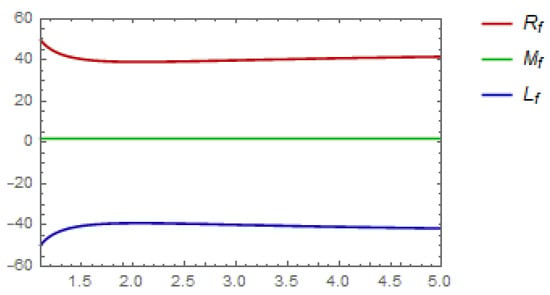
Case one: If we choose $\psi \left(\epsilon \right)=e^{2\epsilon },\epsilon >0$. If we attempt to take $\vartheta {}^{\ast }=1,\varrho {}^{\ast }=2$ and $q\in [1.1,10]$, then the mapping ${\psi }^{″}\left(\epsilon \right)=4e^{2\epsilon }$ is convex for $\epsilon >0$, and we can infer that the inequality in Equation (14) will convert to

$$\begin{array}{cc}\hfill & -\frac{1}{8}·{\left[\frac{2+3\left(\frac{q}{q-1}\right)}{\left(1+\frac{q}{q-1}\right)\left(1+\frac{2q}{q-1}\right)}\right]}^{1-\frac{1}{q}}\left\{{\left[\frac{{\left|4e^2\right|}^q+{\left|4e^4\right|}^q}{2}\right]}^{\frac{1}{q}}+{\left[\frac{{\left|4e^2\right|}^q+{\left|4e^4\right|}^q}{2}\right]}^{\frac{1}{q}}\right\}\hfill \\ \hfill & \le \left\{\frac{e^3}{2}+\frac{e^4+e^2}{4}\right\}-\frac{e^4-e^2}{2}\hfill \\ \hfill & \le \frac{1}{8}·{\left[\frac{2+3\left(\frac{q}{q-1}\right)}{\left(1+\frac{q}{q-1}\right)\left(1+\frac{2q}{q-1}\right)}\right]}^{1-\frac{1}{q}}\left\{{\left[\frac{{\left|4e^2\right|}^q+{\left|4e^4\right|}^q}{2}\right]}^{\frac{1}{q}}+{\left[\frac{{\left|4e^2\right|}^q+{\left|4e^4\right|}^q}{2}\right]}^{\frac{1}{q}}\right\}.\hfill \end{array}$$

(23)

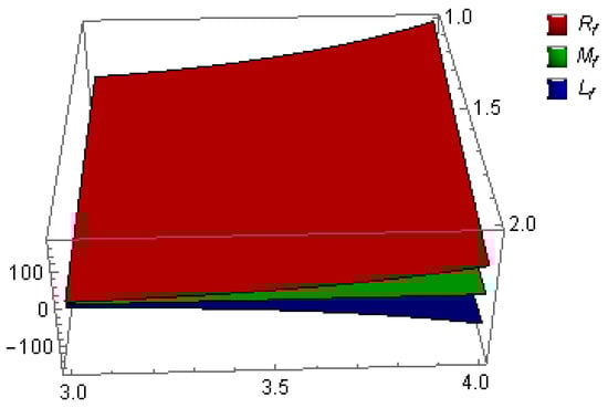
Case two: Let $\psi \left(\epsilon \right)=e^{2\epsilon },\epsilon >0$. If we consider taking $q=2$ and $\vartheta {}^{\ast }\in [1,2],\varrho {}^{\ast }\in [3,4]$, then we can infer that the inequality in Equation (14) will convert to

$$\begin{array}{cc}\hfill & -\frac{1}{8}·{\left(\frac{8}{15}\right)}^{\frac{1}{2}}\left\{{\left[\frac{{\left|4e^{2\vartheta {}^{\ast }}\right|}^2+{\left|4e^{2\varrho {}^{\ast }}\right|}^2}{2}\right]}^{\frac{1}{2}}+{\left[\frac{{\left|4e^{2\vartheta {}^{\ast }}\right|}^2+{\left|4e^{2\varrho {}^{\ast }}\right|}^2}{2}\right]}^{\frac{1}{2}}\right\}\hfill \\ \hfill & \le \left\{\frac{e^{\vartheta {}^{\ast }+\varrho {}^{\ast }}}{2}+\frac{e^{2\varrho {}^{\ast }}+e^{2\vartheta {}^{\ast }}}{4}\right\}-\frac{e^{2\varrho {}^{\ast }}-e^{2\vartheta {}^{\ast }}}{2(\varrho {}^{\ast }-\vartheta {}^{\ast })}\hfill \\ \hfill & \le \frac{1}{8}·{\left(\frac{8}{15}\right)}^{\frac{1}{2}}\left\{{\left[\frac{{\left|4e^{2\vartheta {}^{\ast }}\right|}^2+{\left|4e^{2\varrho {}^{\ast }}\right|}^2}{2}\right]}^{\frac{1}{2}}+{\left[\frac{{\left|4e^{2\vartheta {}^{\ast }}\right|}^2+{\left|4e^{2\varrho {}^{\ast }}\right|}^2}{2}\right]}^{\frac{1}{2}}\right\}.\hfill \end{array}$$

(24)

The three mappings attained in the $R_{\psi },M_{\psi }$ and $L_{\psi }$ in the inequalities in Equation (23) are drawn out in Figure 1 against $q\in [1.1,10]$. The three mappings deduced from the $R_{\psi },M_{\psi }$ and $L_{\psi }$ in the inequalities in Equation (24) are drawn out in Figure 2 against $\vartheta {}^{\ast }\in [1,2],\varrho {}^{\ast }\in [3,4].$

Figure 1. The graphical representation of Example 1 for ${\vartheta }^{\ast }=1$, ${\varrho }^{\ast }=2$ and $q\in [1.1,10]$.

Figure 2. The graphical representation of Example 1 for ${\vartheta }^{\ast }\in [1,2]$, ${\varrho }^{\ast }\in [3,4]$.

Example 2. 

Case one: We choose $\psi \left(\epsilon \right)=\frac{1}{24}{\epsilon }^3,\epsilon >0$. If we consider taking $\vartheta {}^{\ast }=1,\varrho {}^{\ast }=2$ and $q\in [1.1,10]$, then the mapping ${\psi }^{″}\left(\epsilon \right)=\frac{1}{4}\epsilon$ is convex for $\epsilon >0$ and we find that the inequality from Equation (20) will convert to

$$\begin{array}{cc}\hfill & -\frac{1}{96·2^{1-\frac{1}{q}}}·\left\{{\left[{\left(\frac{1}{4}\right)}^{\frac{q}{q-1}}+3·{\left(\frac{1}{2}\right)}^{\frac{q}{q-1}}\right]}^{1-\frac{1}{q}}+{\left[3·{\left(\frac{1}{4}\right)}^{\frac{q}{q-1}}+{\left(\frac{1}{2}\right)}^{\frac{q}{q-1}}\right]}^{1-\frac{1}{q}}\right\}\hfill \\ \hfill & \le \left\{\frac{1}{48}·\left(\frac{27}{8}\right)+\frac{9}{96}\right\}-\frac{15}{96}\approx \frac{1}{128}\hfill \\ \hfill & \le \frac{1}{96·2^{1-\frac{1}{q}}}·\left\{{\left[{\left(\frac{1}{4}\right)}^{\frac{q}{q-1}}+3·{\left(\frac{1}{2}\right)}^{\frac{q}{q-1}}\right]}^{1-\frac{1}{q}}+{\left[3·{\left(\frac{1}{4}\right)}^{\frac{q}{q-1}}+{\left(\frac{1}{2}\right)}^{\frac{q}{q-1}}\right]}^{1-\frac{1}{q}}\right\}.\hfill \end{array}$$

(25)

Case two: Let $\psi \left(\epsilon \right)=\frac{1}{24}{\epsilon }^3,\epsilon >0$. If we consider taking $q=2$ and $\vartheta {}^{\ast }\in [1,2],\varrho {}^{\ast }\in [3,4]$, then we can infer that the inequality from Equation (20) will convert to

$$\begin{array}{cc}\hfill & -\frac{{(\varrho {}^{\ast }-\vartheta {}^{\ast })}^2}{96·2^{\frac{1}{2}}}·\left\{{\left[{\left(\frac{\vartheta {}^{\ast }}{4}\right)}^2+3·{\left(\frac{\varrho {}^{\ast }}{4}\right)}^2\right]}^{\frac{1}{2}}+{\left[3·{\left(\frac{\vartheta {}^{\ast }}{4}\right)}^2+{\left(\frac{\varrho {}^{\ast }}{4}\right)}^2\right]}^{\frac{1}{2}}\right\}\hfill \\ \hfill & \le \left\{\frac{1}{48}·{\left(\frac{\vartheta {}^{\ast }+\varrho {}^{\ast }}{2}\right)}^3+\frac{\varrho {{}^{\ast }}^3+\vartheta {{}^{\ast }}^3}{96}\right\}-\frac{\varrho {{}^{\ast }}^4-\vartheta {{}^{\ast }}^4}{96(\varrho {}^{\ast }-\vartheta {}^{\ast })}\hfill \\ \hfill & \le \frac{{(\varrho {}^{\ast }-\vartheta {}^{\ast })}^2}{96·2^{\frac{1}{2}}}·\left\{{\left[{\left(\frac{\vartheta {}^{\ast }}{4}\right)}^2+3·{\left(\frac{\varrho {}^{\ast }}{4}\right)}^2\right]}^{\frac{1}{2}}+{\left[3·{\left(\frac{\vartheta {}^{\ast }}{4}\right)}^2+{\left(\frac{\varrho {}^{\ast }}{4}\right)}^2\right]}^{\frac{1}{2}}\right\}.\hfill \end{array}$$

(26)

The three mappings attained from the $R_{\psi },M_{\psi }$ and $L_{\psi }$ in the inequalities in Equation (25) are drawn out in Figure 3 against $q\in [1.1,10]$. The three mappings deduced from the $R_{\psi },M_{\psi }$ and $L_{\psi }$ in the inequalities in Equation (26) are drawn out in Figure 4 against $\vartheta {}^{\ast }\in [1,2],\varrho {}^{\ast }\in [3,4].$

Figure 3. The graphical representation of Example 2 for ${\vartheta }^{\ast }=1$, ${\varrho }^{\ast }=2$ and $q\in [1.1,10]$.

Figure 4. The graphical representation of Example 2 for ${\vartheta }^{\ast }\in [1,2]$, ${\varrho }^{\ast }\in [3,4]$.

Comparative Analysis of Classical and Improved Bounds

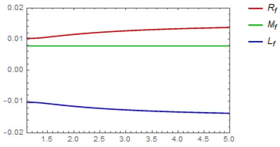
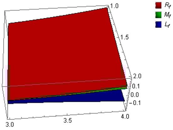
Example 3. 

If we choose $\psi \left(\epsilon \right)=\frac{1}{12}{\epsilon }^4,\epsilon >0$, then $|{\psi }^{″}{\left(\epsilon \right)|}^q=varepsilo{n}^4$ for $q>1$ and $\epsilon >0$ is a convex function. For the case where $\alpha =1,\vartheta {}^{\ast }=1,\varrho {}^{\ast }=2$ and $q=2,$ let us find the right part of the inequalities from Equations (14) and (16).

(a) 

For Equation (14), we have

$$\begin{array}{cc}\hfill & \left|\frac{1}{2}\left[\psi \left(\frac{\vartheta {}^{\ast }+\varrho {}^{\ast }}{2}\right)+\frac{\psi \left(\varrho {}^{\ast }\right)+\psi \left(\vartheta {}^{\ast }\right)}{2}\right]-\frac{1}{\varrho {}^{\ast }-\vartheta {}^{\ast }}{\int }_{\vartheta {}^{\ast }}^{\varrho {}^{\ast }}\psi \left(t\right)dt\right|\hfill \\ \hfill & \le \frac{{\left(\varrho {}^{\ast }-\vartheta {}^{\ast }\right)}^2}{8}{\mathbf{S}}^{\frac{1}{p}}\left\{{\left[\frac{|{\psi }^{″}\left(\vartheta {}^{\ast }\right){|}^q}{2}+\frac{3|{\psi }^{″}\left(\varrho {}^{\ast }\right){|}^q}{2}\right]}^{\frac{1}{q}}\right.\hfill \\ \hfill & \left.+{\left[\frac{3|{\psi }^{″}\left(\vartheta {}^{\ast }\right){|}^q}{2}+\frac{|{\psi }^{″}\left(\varrho {}^{\ast }\right){|}^q}{2}\right]}^{\frac{1}{q}}\right\}\hfill \\ \hfill & =\frac{1}{8}{\left(\frac{8}{15}\right)}^{\frac{1}{2}}\left\{{\left[\frac{1}{2}+24\right]}^{\frac{1}{2}}+{\left[\frac{3}{2}+8\right]}^{\frac{1}{2}}\right\}\hfill \\ \hfill & \approx 0.733214.\hfill \end{array}$$

(b) 

For Equation (16), we have

$$\begin{array}{cc}\hfill & \left|\frac{1}{2}\left[\psi \left(\frac{\vartheta {}^{\ast }+\varrho {}^{\ast }}{2}\right)+\frac{\psi \left(\varrho {}^{\ast }\right)+\psi \left(\vartheta {}^{\ast }\right)}{2}\right]-\frac{1}{\varrho {}^{\ast }-\vartheta {}^{\ast }}{\int }_{\vartheta {}^{\ast }}^{\varrho {}^{\ast }}\psi \left(t\right)dt\right|\hfill \\ \hfill & \le \frac{{\left(\varrho {}^{\ast }-\vartheta {}^{\ast }\right)}^2}{16}{B}^{\frac{1}{2}}\left(3,4\right)\left\{\widetilde{{\mathbf{M}}_1}+\widetilde{{\mathbf{M}}_3}+\widetilde{{\mathbf{M}}_2}+\widetilde{{\mathbf{M}}_4}\right\}\hfill \\ \hfill & =\frac{1}{16}\left[0.12909·\left\{2.598076+2.345208+1.322876+1.732051\right\}\right]\hfill \\ \hfill & \approx 0.064530.\hfill \end{array}$$

Since $0.733214>0.064530,$ the extended Hölder inequality gives a better estimate than the classical Hölder inequality. The 2D and 3D graphical illustrations of Example 3 are mentioned in Figure 5 and Figure 6, respectively.

Example 4. 

If we choose $\psi \left(\epsilon \right)=e^{\epsilon },\epsilon >0$, then $|{\psi }^{″}{\left(\epsilon \right)|}^q$ = $e^{\epsilon }$ for $q>1$ and $\epsilon >0$ is a convex function. For the case where $\alpha =1,\vartheta {}^{\ast }=1,\varrho {}^{\ast }=2$ and $q=2,$ let us find the right part of the inequalities from Equations (20) and (22).

(a) 

For Equation (20), we have

$$\begin{array}{cc}\hfill & \left|\frac{1}{2}\left[\psi \left(\frac{\vartheta {}^{\ast }+\varrho {}^{\ast }}{2}\right)+\frac{\psi \left(\varrho {}^{\ast }\right)+\psi \left(\vartheta {}^{\ast }\right)}{2}\right]-\frac{1}{\varrho {}^{\ast }-\vartheta {}^{\ast }}{\int }_{\vartheta {}^{\ast }}^{\varrho {}^{\ast }}\psi \left(\epsilon \right)d\epsilon \right|\hfill \\ \hfill & \le \frac{{\left(\varrho {}^{\ast }-\vartheta {}^{\ast }\right)}^2}{96·2^{\frac{1}{p}}}\left\{{\left[{\left|{\psi }^{″}\left(\vartheta {}^{\ast }\right)\right|}^p+3{\left|{\psi }^{″}\left(\varrho {}^{\ast }\right)\right|}^p\right]}^{\frac{1}{p}}+{\left[3{\left|{\psi }^{″}\left(\vartheta {}^{\ast }\right)\right|}^p+{\left|{\psi }^{″}\left(\varrho {}^{\ast }\right)\right|}^p\right]}^{\frac{1}{p}}\right\}\hfill \\ \hfill & =\frac{1}{96·2^{\frac{1}{2}}}·\left[{\left(7.3891+163.7944\right)}^{\frac{1}{2}}+{\left(22.16716+54.5981\right)}^{\frac{1}{2}}\right]\hfill \\ \hfill & \approx 0.1609.\hfill \end{array}$$

(b) 

For Equation (22), we have

$$\begin{array}{cc}\hfill & \left|\frac{1}{2}\left[\psi \left(\frac{\vartheta {}^{\ast }+\varrho {}^{\ast }}{2}\right)+\frac{\psi \left(\varrho {}^{\ast }\right)+\psi \left(\vartheta {}^{\ast }\right)}{2}\right]-\frac{1}{\varrho {}^{\ast }-\vartheta {}^{\ast }}{\int }_{\vartheta {}^{\ast }}^{\varrho {}^{\ast }}\psi \left(\epsilon \right)d\epsilon \right|\hfill \\ \hfill & \le \frac{{(\varrho {}^{\ast }-\vartheta {}^{\ast })}^2}{16}{\left(\frac{1}{12}\right)}^{1-\frac{1}{q}}\left[{\left\{\frac{{\left|{\psi }^{″}\left(\varrho {}^{\ast }\right)\right|}^q}{10}-\frac{{\left|{\psi }^{″}\left(\vartheta {}^{\ast }\right)\right|}^q}{60}\right\}}^{\frac{1}{q}}+{\left\{\frac{{\left|{\psi }^{″}\left(\varrho {}^{\ast }\right)\right|}^q}{60}-\frac{{\left|{\psi }^{″}\left(\vartheta {}^{\ast }\right)\right|}^q}{15}\right\}}^{\frac{1}{q}}\right.\hfill \\ \hfill & \left.+{\left\{\frac{13{\left|{\psi }^{″}\left(\varrho {}^{\ast }\right)\right|}^q}{120}-\frac{{\left|{\psi }^{″}\left(\vartheta {}^{\ast }\right)\right|}^q}{40}\right\}}^{\frac{1}{q}}+{\left\{\frac{{\left|{\psi }^{″}\left(\varrho {}^{\ast }\right)\right|}^q}{40}-\frac{7{\left|{\psi }^{″}\left(\vartheta {}^{\ast }\right)\right|}^q}{120}\right\}}^{\frac{1}{q}}\right].\hfill \\ \hfill & =\frac{1}{16}0.2887·\left[2.310122+0.646038+2.393757+0.966398\right]\hfill \\ \hfill & \approx 0.113958.\hfill \end{array}$$

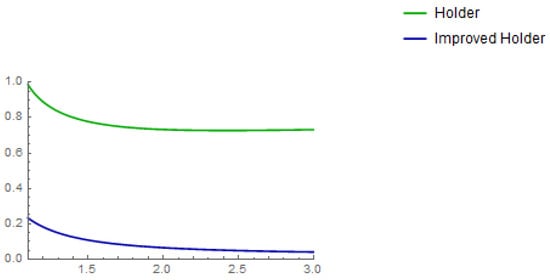
Figure 5. The graphical representation of Example 3 for ${\vartheta }^{\ast }=1$, ${\varrho }^{\ast }=2$ and $q\in [1.1,10]$.

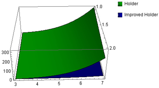
Figure 6. The graphical representation of Example 3 for ${\vartheta }^{\ast }\in [1,2]$, ${\varrho }^{\ast }\in [3,7]$.

Since $0.1609>0.113958$, the extended power mean inequality gives a better estimate than the classical power mean inequality. The 2D and 3D graphical illustrations of Example 4 are mentioned in Figure 7 and Figure 8, respectively.

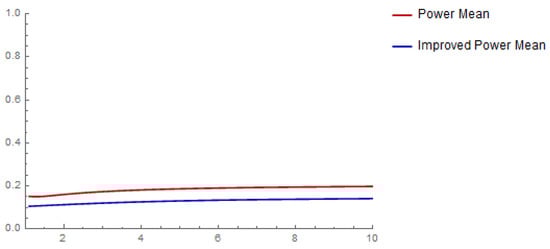
Figure 7. The graphical representation of Example 4 for ${\vartheta }^{\ast }=1,{\varrho }^{\ast }=2$ and $q\in [1.1,10]$.

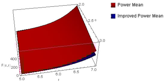
Figure 8. The graphical representation of Example 4 for ${\vartheta }^{\ast }\in [2,3],{\varrho }^{\ast }\in [5,7]$.

4. Applications

In this section, we employ our obtained results to derive some notable applications in terms of special means, the quadrature rule and estimations of inequalities in terms of special functions.

4.1. Special Means

We here consider the means for arbitrary real numbers $\vartheta {}^{\ast },\varrho {}^{\ast }$$(\vartheta {}^{\ast }\ne \varrho {}^{\ast }).$ We use the following:

• $Arithmetic$ $mean$:

  $$A(\vartheta {}^{\ast },\varrho {}^{\ast })=\frac{\vartheta {}^{\ast }+\varrho {}^{\ast }}{2},\vartheta {}^{\ast },\varrho {}^{\ast }\in \mathbb{R}.$$
• $Logarithmic$ $mean$:

  $$L(\vartheta {}^{\ast },\varrho {}^{\ast })=\frac{\vartheta {}^{\ast }-\varrho {}^{\ast }}{ln\left|\vartheta {}^{\ast }\right|-ln\left|\varrho {}^{\ast }\right|},\left|\vartheta {}^{\ast }\right|\ne \left|{\varrho }^{\ast }\right|,\vartheta {}^{\ast },\varrho {}^{\ast }\ne 0,\vartheta {}^{\ast },\varrho {}^{\ast }\in \mathbb{R}.$$
• $Generalized$ log-mean:

  $$L_n(\vartheta {}^{\ast },\varrho {}^{\ast })={\left[\frac{{\left(\varrho {}^{\ast }\right)}^{n+1}-{\left(\vartheta {}^{\ast }\right)}^{n+1}}{(n+1)(\varrho {}^{\ast }-{\vartheta }^{\ast })}\right]}^{\frac{1}{n}},n\in Z\setminus \{-1,0\},\vartheta {}^{\ast },\varrho {}^{\ast }\in {\mathbb{R}}^{+}.$$
• $Harmonic$ mean:

  $$H=H(\vartheta {}^{\ast },\varrho {}^{\ast })=\frac{2\vartheta {}^{\ast }\varrho {}^{\ast }}{\vartheta {}^{\ast }+\varrho {}^{\ast }};\vartheta {}^{\ast },\varrho {}^{\ast }>0.$$
• p-Logarithmic $mean$:

  $$L_p(\vartheta {}^{\ast },\varrho {}^{\ast })={\left(\frac{{\left({\varrho }^{\ast }\right)}^{1+p}-{\left({\vartheta }^{\ast }\right)}^{1+p}}{\left(1+p\right)\left(\varrho {}^{\ast }-\vartheta {}^{\ast }\right)}\right)}^{\frac{1}{p}},p\in \mathbb{R}-\{-1,0\},{\vartheta }^{\ast },{\varrho }^{\ast }>0.$$

Proposition 1. 

Let $\vartheta {}^{\ast },{\varrho }^{\ast }$$\in [0,\infty )$, $\vartheta {}^{\ast }<{\varrho }^{\ast }$ and $n\in {\mathbb{Z}}^{+}$, $n\ge 2$. Then, we have

$$\begin{array}{cc}\hfill & \left|L_n^n-\frac{1}{2}\left[A^n\left(\vartheta {}^{\ast },{\varrho }^{\ast }\right)+A\left(\vartheta {{}^{\ast }}^n,{{\varrho }^{\ast }}^n\right)\right]\right|\hfill \\ \hfill & \le \frac{n(n-1){({\varrho }^{\ast }-\vartheta {}^{\ast })}^2}{8}{S}^{\frac{1}{p}}\left\{A^{\frac{1}{q}}\left(|\vartheta {}^{\ast }{|}^{(n-2)q},3{|{\varrho }^{\ast }|}^{(n-2)q}\right)+A^{\frac{1}{q}}\left(3|\vartheta {}^{\ast }{|}^{(n-2)q},{|{\varrho }^{\ast }|}^{(n-2)q}\right)\right\},\hfill \end{array}$$

where

$$\mathbf{S}=\frac{2+3p}{(1+p)(1+2p)}.$$

Proof. 

This follows from Corollary 2 applied to the convex function

$$\begin{array}{c}\hfill \psi \left(\epsilon \right)={\epsilon }^n,\psi :[0,\infty )\to \mathbb{R}.\end{array}$$

□

Proposition 2. 

Let $\vartheta {}^{\ast },{\varrho }^{\ast }\in \mathbb{R}$ with $0<\vartheta {}^{\ast }<{\varrho }^{\ast }$. Then,

$$\begin{array}{cc}\hfill & \left|L^{-1}\left(\vartheta {}^{\ast },{\varrho }^{\ast }\right)-\frac{1}{2}\left[A^{-1}\left(\vartheta {}^{\ast },{\varrho }^{\ast }\right)+H^{-1}\left(\vartheta {}^{\ast },{\varrho }^{\ast }\right)\right]\right|\hfill \\ \hfill & \le \frac{{({\varrho }^{\ast }-\vartheta {}^{\ast })}^2}{2^{3-\frac{1}{q}}}{S}^{\frac{1}{p}}\left\{A^{\frac{1}{q}}\left(|\vartheta {}^{\ast }{|}^{-3q},3{|{\varrho }^{\ast }|}^{-3q}\right)+A^{\frac{1}{q}}\left(3|\vartheta {}^{\ast }{|}^{-3q},{|{\varrho }^{\ast }|}^{-3q}\right)\right\}.\hfill \end{array}$$

Proof. 

This follows from Corollary 2 applied to the convex function

$$\psi \left(\epsilon \right)=\frac{1}{\epsilon },\epsilon \ne 0.$$

□

Proposition 3. 

Let $\vartheta {}^{\ast },{\varrho }^{\ast }$$\in [0,\infty ),\vartheta {}^{\ast }<{\varrho }^{\ast }$, ∀$q>1$. Then, we have

$$\begin{array}{cc}\hfill & \left|L\left(\vartheta {}^{\ast },{\varrho }^{\ast }\right)-\frac{1}{2}\left[e^{A(\vartheta {}^{\ast },{\varrho }^{\ast })}+A\left(e^{\vartheta {}^{\ast }},e^{{\varrho }^{\ast }}\right)\right]\right|\hfill \\ \hfill & \le \frac{{({\varrho }^{\ast }-\vartheta {}^{\ast })}^2}{8}{S}^{\frac{1}{p}}\left\{A^{\frac{1}{q}}\left({|e|}^{\vartheta {}^{\ast }q},3{|e|}^{{\varrho }^{\ast }q}\right)+A^{\frac{1}{q}}\left({3|e|}^{\vartheta {}^{\ast }q},{|e|}^{{\varrho }^{\ast }q}\right)\right\}.\hfill \end{array}$$

Proof. 

This follows from Corollary 2 applied to the convex function

$$\psi \left(\epsilon \right)=e^{\epsilon },\psi :[0,\infty )\to \mathbb{R}.$$

□

Proposition 4. 

Let $\vartheta {}^{\ast },\varrho {}^{\ast }$$\in [0,\infty )$, $\vartheta {}^{\ast }<\varrho {}^{\ast }$ and $n\in {\mathbb{Z}}^{+}$, $n\ge 2$. Then, we have

$$\begin{array}{cc}\hfill & \left|L_n^n\left(\vartheta {}^{\ast },\varrho {}^{\ast }\right)-\frac{1}{2}\left[A^n\left(\vartheta {}^{\ast },\varrho {}^{\ast }\right)+A\left(\vartheta {{}^{\ast }}^n,\varrho {{}^{\ast }}^n\right)\right]\right|\hfill \\ \hfill & \le \frac{{(\varrho {}^{\ast }-\vartheta {}^{\ast })}^2}{96}n(n-1)\left[A^{\frac{1}{p}}\left(|\vartheta {}^{\ast }{|}^{(n-2)p},3{|\varrho {}^{\ast }|}^{(n-2)p}\right)+A^{\frac{1}{p}}\left(3|\vartheta {}^{\ast }{|}^{(n-2)p},{|\varrho {}^{\ast }|}^{(n-2)p}\right)\right].\hfill \end{array}$$

Proof. 

This follows from Corollary 4 applied to the convex function

$$\psi \left(\epsilon \right)={\epsilon }^n,\psi :[0,\infty )\to \mathbb{R}.$$

□

Proposition 5. 

Let $\vartheta {}^{\ast },\varrho {}^{\ast }\in \mathbb{R}$ with $0<\vartheta {}^{\ast }<\varrho {}^{\ast }$. Then,

$$\begin{array}{cc}\hfill & \left|L^{-1}\left(\vartheta {}^{\ast },\varrho {}^{\ast }\right)-\frac{1}{2}\left[A^{-1}\left(\vartheta {}^{\ast },\varrho {}^{\ast }\right)+H^{-1}\left(\vartheta {}^{\ast },\varrho {}^{\ast }\right)\right]\right|\hfill \\ \hfill & \le \frac{{(\varrho {}^{\ast }-\vartheta {}^{\ast })}^2}{96}\left[A^{\frac{1}{p}}\left(|\vartheta {}^{\ast }{|}^{-3p},3{|\varrho {}^{\ast }|}^{-3p}\right)+A^{\frac{1}{p}}\left(3|\vartheta {}^{\ast }{|}^{-3p},{|{\varrho }^{\ast }|}^{-3p}\right)\right].\hfill \end{array}$$

Proof. 

This follows from Corollary 4 applied to the convex function

$$\psi \left(\epsilon \right)=\frac{1}{\epsilon },\epsilon \ne 0.$$

□

4.2. Quadrature Formula

Here, we present an application to a quadrature formula. Let $d$ be a partition $\vartheta {}^{\ast }={\epsilon }_0<{\epsilon }_1\dots <{\epsilon }_{m-1}<{\epsilon }_m=\varrho {}^{\ast }$ of the interval $[\vartheta {}^{\ast },\varrho {}^{\ast }]$ and consider the quadrature formula

$${\int }_{\vartheta {}^{\ast }}^{\varrho {}^{\ast }}\psi \left(\epsilon \right)d\epsilon =T(\psi ,d)+E(\psi ,d),$$

where

$$T(\psi ,d)=\sum _{i=0}^{m-1}\frac{\left({\epsilon }_{i+1}-{\epsilon }_i\right)}{2}\left[\frac{\psi \left({\epsilon }_i\right)+\psi \left({\epsilon }_{i+1}\right)}{2}+\psi \left(\frac{{\epsilon }_i+{\epsilon }_{i+1}}{2}\right)\right],$$

(27)

is the quadrature version and $E(\psi ,d)$ is the approximation error. Here, we present some error estimates for the quadrature formula.

Proposition 6. 

Under the condition of Corollary 1, the following inequality is true:

$$\left|{\int }_{\vartheta {}^{\ast }}^{\varrho {}^{\ast }}\psi \left(\epsilon \right)d\epsilon -T(\psi ,d)\right|\le \sum _{i=0}^{m-1}\frac{{({\epsilon }_{i+1}-{\epsilon }_i)}^3}{96}\left[\left|{\psi }^{″}\left({\epsilon }_{i+1}\right)\right|+\left|{\psi }^{″}\left({\epsilon }_i\right)\right|\right].$$

(28)

Proof. 

Apply Corollary 1 and we get the desired result. □

Remark 3. 

If the d-fragmentation of the interval $[\vartheta {}^{\ast },\varrho {}^{\ast }]$ is uniform, then, from Equations (27) and (28), we get

$$T(\psi ,d)=\frac{h}{2}\sum _{i=0}^{m-1}\left[\frac{\psi \left({\epsilon }_i\right)+\psi \left({\epsilon }_{i+1}\right)}{2}+\psi \left(\frac{{\epsilon }_i+{\epsilon }_{i+1}}{2}\right)\right],$$

and

$$\left|{\int }_{\vartheta {}^{\ast }}^{\varrho {}^{\ast }}\psi \left(\epsilon \right)d\epsilon -T(\psi ,d)\right|\le \frac{m{h}^3}{48}{M}_2\le \frac{m^3{h}^3}{48}{M}_2=\frac{{\left(\varrho {}^{\ast }-\vartheta {}^{\ast }\right)}^3}{48}{M}_2,$$

where $h={\epsilon }_{i+1}-{\epsilon }_i$ and $M_2=\underset{x\in [\vartheta {}^{\ast },{\varrho }^{\ast }]}{max}\left(\left|{\psi }^{″}\left(x\right)\right|\right).$

The resulting error is better than the errors expressed in terms of the second derivatives of the Newton–Cotes (midpoint or trapezoid formula) and Gauss quadrature formulas:

$$R_1\left(\psi \right)=\frac{M_2}{24}{\left(\varrho {}^{\ast }-\vartheta {}^{\ast }\right)}^3,or{R}_2\left(\psi \right)=\frac{M_2}{12}{\left(\varrho {}^{\ast }-\vartheta {}^{\ast }\right)}^3,$$

and

$$R_{2n}\left(\psi \right)=\frac{M_{2n}{(n!)}^4}{{(\left(2n\right)!)}^3(2n+1)}{\left(\varrho {}^{\ast }-\vartheta {}^{\ast }\right)}^3,M_{2n}=\underset{x\in [\vartheta {}^{\ast },{\varrho }^{\ast }]}{max}\left(\left|{\psi }^{\left(2n\right)}\left(x\right)\right|\right),forn=1$$

respectively.

Proposition 7. 

Let ψ:$[\vartheta {}^{\ast },\varrho {}^{\ast }]\to \mathbb{R}$ be the differentiable mapping on $(\vartheta {}^{\ast },\varrho {}^{\ast })$ with $\vartheta {}^{\ast }<\varrho {}^{\ast }$. Suppose that $|{\psi }^{″}{|}^q$, $q\ge 1$ is a convex function; then, for every partition of $[\vartheta {}^{\ast },\varrho {}^{\ast }]$, the midpoint error satisfies

$$\begin{array}{cc}\hfill & \left|{\int }_{\vartheta {}^{\ast }}^{\varrho {}^{\ast }}\psi \left(\epsilon \right)d\epsilon -T(\psi ,d)\right|\le \frac{B^{\frac{1}{p}}(1+p,2+p)}{16}\hfill \\ \hfill & \times \sum _{i=0}^{m-1}{({\epsilon }_{i+1}-{\epsilon }_i)}^3\left[{\left(\frac{|{\psi }^{″}\left({\epsilon }_i\right){|}^q+5{|{\psi }^{″}\left({\epsilon }_{i+1}\right)|}^q}{12}\right)}^{\frac{1}{q}}+{\left(\frac{|{\psi }^{″}\left({\epsilon }_{i+1}\right){|}^q+5{|{\psi }^{″}\left({\epsilon }_i\right)|}^q}{12}\right)}^{\frac{1}{q}}\right.\hfill \\ \hfill & \left.+{\left(\frac{|{\psi }^{″}\left({\epsilon }_i\right){|}^q+2{|{\psi }^{″}\left({\epsilon }_{i+1}\right)|}^q}{6}\right)}^{\frac{1}{q}}+{\left(\frac{|{\psi }^{″}\left({\epsilon }_{i+1}\right){|}^q+2{|{\psi }^{″}\left({\epsilon }_i\right)|}^q}{6}\right)}^{\frac{1}{q}}\right].\hfill \end{array}$$

Proof. 

Apply Corollary 3 and then we get the desired result. □

4.3. $\tilde{\mathbf{q}}$-Digamma Function

The $\tilde{q}$-digamma mapping is determined by the expression below [34]:

$${\delta }_{\tilde{q}}\left(\epsilon \right)=-ln(\tilde{q}-1)+ln\left(\tilde{q}\right)\left(\epsilon -\frac{1}{2}-\sum _{j=1}^{\infty }\frac{{\tilde{q}}^{-j\epsilon }}{1-{\tilde{q}}^{-j\epsilon }}\right),$$

with $\tilde{q}>1$ and $\epsilon >0.$

Proposition 8. 

For $0<\vartheta {}^{\ast }<\varrho {}^{\ast }$, we get

$$\begin{array}{cc}\hfill & \left|\frac{1}{2}\left[{\delta }_{\tilde{q}}^{\prime }\left(\frac{\vartheta {}^{\ast }+\varrho {}^{\ast }}{2}\right)+\frac{{\delta }_{\tilde{q}}^{\prime }\left(\varrho {}^{\ast }\right)+{\delta }_{\tilde{q}}^{\prime }\left(\vartheta {}^{\ast }\right)}{2}\right]-\frac{{\delta }_{\tilde{q}}\left(\varrho {}^{\ast }\right)-{\delta }_{\tilde{q}}\left(\vartheta {}^{\ast }\right)}{{\varrho }^{\ast }-\vartheta {}^{\ast }}\right|\hfill \\ \hfill & \le \frac{{(\varrho {}^{\ast }-\vartheta {}^{\ast })}^2}{96}\left[\left|{\delta }_{\tilde{q}}^{‴}\left(\vartheta {}^{\ast }\right)\right|+\left|{\delta }_{\tilde{q}}^{‴}\left(\varrho {}^{\ast }\right)\right|\right].\hfill \end{array}$$

Proof. 

Applying $\psi \left(\epsilon \right)={\delta }_{\tilde{q}}^{\prime }\left(\epsilon \right)$ for $\epsilon >0$ to Corollary 1, we obtain the desired result. □

Proposition 9. 

For $0<\vartheta {}^{\ast }<\varrho {}^{\ast },q>1$ and $\frac{1}{p}+\frac{1}{q}=1,$ we get that

$$\begin{array}{cc}\hfill & \left|\frac{1}{2}\left[{\delta }_{\tilde{q}}^{\prime }\left(\frac{\vartheta {}^{\ast }+\varrho {}^{\ast }}{2}\right)+\frac{{\delta }_{\tilde{q}}^{\prime }\left(\varrho {}^{\ast }\right)+{\delta }_{\tilde{q}}^{\prime }\left(\vartheta {}^{\ast }\right)}{2}\right]-\frac{{\delta }_{\tilde{q}}\left(\varrho {}^{\ast }\right)-{\delta }_{\tilde{q}}\left(\vartheta {}^{\ast }\right)}{{\varrho }^{\ast }-\vartheta {}^{\ast }}\right|\hfill \\ \hfill & \le \frac{{(\varrho {}^{\ast }-\vartheta {}^{\ast })}^2}{96}\left[{\left({\left|{\delta }_{\tilde{q}}^{‴}\left(\vartheta {}^{\ast }\right)\right|}^p+3{\left|{\delta }_{\tilde{q}}^{‴}\left(\varrho {}^{\ast }\right)\right|}^p\right)}^{\frac{1}{p}}+{\left(3{\left|{\delta }_{\tilde{q}}^{‴}\left(\vartheta {}^{\ast }\right)\right|}^p+{\left|{\delta }_{\tilde{q}}^{‴}\left(\varrho {}^{\ast }\right)\right|}^p\right)}^{\frac{1}{p}}\right].\hfill \end{array}$$

Proof. 

Applying $\psi \left(\epsilon \right)={\delta }_{\tilde{q}}^{\prime }\left(\epsilon \right)$ for $\epsilon >0$ to Corollary 4, we obtain the desired result. □

4.4. Modified Bessel Function

Let the function ${\mathcal{I}}_p:\mathbb{R}\to [1,0)$ be defined by

$${\mathcal{I}}_p\left(\epsilon \right)=2^p\Gamma (1+p){\epsilon }^{-{\varrho }^{\ast }}{I}_p\left(\epsilon \right),$$

For this, we recall the modified Bessel function of the first kind $I_p$, which is defined as [35]:

$$I_p\left(\epsilon \right)=\sum _{n\ge 0}\frac{{\left(\frac{\epsilon }{2}\right)}^{p+2n}}{n!\Gamma (p+n+1)}.$$

The first- and nth-order derivative formulas of ${\mathcal{I}}_p\left(\epsilon \right)$ are, respectively [36]:

$$\begin{array}{cc}\hfill & {\mathcal{I}}_p^{\prime }\left(\epsilon \right)=\frac{\epsilon }{2(1+p)}{\mathcal{I}}_{1+p}\left(\epsilon \right),\hfill \\ \hfill & \frac{{\partial }^n{\mathcal{I}}_p\left(\epsilon \right)}{{\partial }^n\epsilon }=2^{n-2p}\sqrt{\pi }{\epsilon }^{p-n}\Gamma {(1+p)}_2{F}_3\left(\frac{1+p}{2},\frac{2+p}{2};\frac{1+p-n}{2},1+p;\frac{{\epsilon }^2}{4}\right),\hfill \end{array}$$

where ${}_2{F}_3(.,.,.)$ is the hypergeometric function defined by [36]:

$${}_2{F}_3\left(\frac{1+p}{2},\frac{2+p}{2};\frac{1+p-n}{2},1+p;\frac{{\epsilon }^2}{4}\right)=\sum _{k=0}^{\infty }\frac{{\left(\frac{1+p}{2}\right)}_k{\left(\frac{1+p}{2}\right)}_k}{{\left(\frac{p-2}{2}\right)}_k{\left(\frac{p-1}{2}\right)}_k{(1+p)}_k}\frac{{\epsilon }^{2k}}{4^k\left(k\right)!}.$$

Proposition 10. 

Let $\vartheta {}^{\ast },\varrho {}^{\ast }\in \mathbb{R}$ with $0<\vartheta {}^{\ast }<\varrho {}^{\ast }$; then, for each $p>-1$, we have

$$\begin{array}{cc}\hfill & \left|\frac{1}{2}\left[\frac{\vartheta {}^{\ast }+\varrho {}^{\ast }}{4(1+p)}{\mathcal{I}}_{1+p}\left(\frac{\vartheta {}^{\ast }+\varrho {}^{\ast }}{2}\right)+\frac{\varrho {}^{\ast }{\mathcal{I}}_{1+p}\left(\varrho {}^{\ast }\right)+\vartheta {}^{\ast }{\mathcal{I}}_{1+p}\left(\vartheta {}^{\ast }\right)}{4(1+p)}\right]-\frac{{\mathcal{I}}_p\left(\varrho {}^{\ast }\right)-{\mathcal{I}}_p\left(\vartheta {}^{\ast }\right)}{\varrho {}^{\ast }-\vartheta {}^{\ast }}\right|\hfill \\ \hfill & \le \frac{{(\varrho {}^{\ast }-\vartheta {}^{\ast })}^2}{96}{2}^{3-2p}\sqrt{\pi }\Gamma (1+p)\times \left(|\vartheta {}^{\ast }{|}^{p-3}\left|{}_2{F}_3\left(\frac{1+p}{2},\frac{2+p}{2};\frac{p-2}{2},\frac{p-1}{2},1+p;\frac{{\left({\vartheta }^{\ast }\right)}^2}{4}\right)\right|\right.\hfill \\ \hfill & \left.+|\varrho {}^{\ast }{|}^{p-3}\left|{}_2{F}_3\left(\frac{1+p}{2},\frac{2+p}{2};\frac{p-2}{2},\frac{p-1}{2},1+p;\frac{{\left({\varrho }^{\ast }\right)}^2}{4}\right)\right|\right).\hfill \end{array}$$

Proof. 

Applying $\psi \left(\epsilon \right)$ = ${\mathcal{I}}_p^{\prime }\left(\epsilon \right)$ to Corollary 1, we get the desired result. □

5. Concluding Remarks

In this study, we first developed a new fractional Bullen-type identity with a parameter. Thus employing the theory of convexity, we provided new estimations of fractional Bullen-type inequalities pertaining to twice-differentiable functions. An analysis of the improvement of the estimations was provided using several concrete examples with graphical visualizations. Finally, several applications were provided as well. This study could be used to explore for other general fractional integral operators with non-singular kernels. Also, one can think about studying such results for other classes of convex functions, especially coordinate convex functions.

References

- Mitrinovic, D.S.; Pećarixcx, J.; Fink, A.M. Classical and New Inequalities in Analysis; Mathematics and Its Applications (East European Series); Kluwer Academic Publishers Group: Dordrecht, The Netherlands, 1993; Volume 61. [Google Scholar]
- Dragomir, S.S.; Pearse, C.E.M. Selected Topics on Hermite-Hadamard Inequalities and Applications; RGMIA Monograps; Victoria University: Footscray, VIC, Australia, 2000. [Google Scholar]
- Rasheed, T.; Butt, S.I.; Pečarić, D.; Pečarić, J. Generalized Cyclic Jensen and Information Inequalities. Chaos Solitons Fractals 2022, 163, 112602. [Google Scholar] [CrossRef]
- Gasimov, Y.S.; Nápoles, J.E. Some refinements of Hermite-Hadamard inequality using k-fractional Caputo derivatives. Fract. Differ. Calc. 2022, 12, 209–221. [Google Scholar] [CrossRef]
- Agarwal, P.; Dragomir, S.S.; Jleli, M.; Samet, B. (Eds.) Advances in Mathematical Inequalities and Applications; Springer: Singapore, 2018. [Google Scholar]
- Qin, Y. Integral and Discrete Inequalities and Their Applications; Springer International Publishing: Basel, Switzerland, 2016. [Google Scholar]
- Fahad, A.; Ayesha; Wang, Y.; Butt, S.I. Jensen-Mercer and Hermite-Hadamard-Mercer Type Inequalities for GA-h-Convex Functions and Its Subclasses with Applications. Mathematics 2023, 11, 278. [Google Scholar] [CrossRef]
- Pečarić, J.; Tong, Y.L. Convex Functions, Partial Orderings, and Statistical Applications; Academic Press: Cambridge, MA, USA, 1992. [Google Scholar]
- Tariq, M.; Ntouyas, S.K.; Shaikh, A.A. New Variant of Hermite-Hadamard, Fejér and Pachpatte-Type Inequality and Its Refinements Pertaining to Fractional Integral Operator. Fractal Fract. 2023, 7, 405. [Google Scholar] [CrossRef]
- Nápoles, J.E.; Bayraktar, B. On the generalized inequalities of the Hermite-Hadamard type. Filomat 2021, 35, 4917–4924. [Google Scholar] [CrossRef]
- Bayraktar, B.; Gürbüz, B. On some integral inequalities for (s,m)- convex functions. TWMS J. Appl. Eng. Math. 2020, 10, 288–295. [Google Scholar]
- Bullen, P.S. Error Estimates for Some Elementary Quadrature Rules; No. 602/633; University of Belgrade: Belgrade, Serbia, 1978; pp. 97–103. [Google Scholar]
- Tseng, K.-L.; Hwang, S.-R.; Hsua, K.-C. Hadamard-type and Bullen-type inequalities for Lipschitzian functions and their applications. Comput. Math. Appl. 2012, 64, 651–660. [Google Scholar] [CrossRef]
- Çakmak, M. The differentiable h-convex functions involving the Bullen inequality. Acta Univ. Apulensis 2021, 65, 29–36. [Google Scholar]
- Erden, S.; Sarikaya, M.Z. Generalized Bullen-type inequalities for local fractional integrals and its applications. Palest. J. Math 2020, 9, 945–956. [Google Scholar]
- Sarikaya, M.Z.; Tunc, T.; Budak, H. On generalized some integral inequalities for local fractional integrals. Appl. Math. Comput. 2016, 276, 316–323. [Google Scholar]
- Işcan, T.; Toplu, T.; Yetgin, F. Some new inequalities on generalization of Hermite-Hadamard and Bullen type inequalities, applications to trapezoidal and midpoint formula. Kragujev. J. Math. 2021, 45, 647–657. [Google Scholar] [CrossRef]
- Hussain, S.; Mehboob, S. On some generalized fractional integral Bullen type inequalities with applications. J. Fract. Calc. Nonlinear Syst. 2021, 2, 93–112. [Google Scholar] [CrossRef]
- Yaşar, B.N.; Aktan, N.; Kizilkan, G.Ç. Generalization of Bullen type, trapezoid type, midpoint type and Simpson type inequalities for s-convex in the fourth sense. Turk. J. Inequal. 2022, 6, 40–51. [Google Scholar]
- Boulares, H.; Meftah, B.; Moumen, A.; Shafqat, R.; Saber, H.; Alraqad, T.; Ali, E. Fractional multiplicative Bullen-type inequalities for multiplicative differentiable functions. Symmetry 2023, 15, 451. [Google Scholar] [CrossRef]
- Bayraktar, B.; Butt, S.I.; Napoles, J.E.; Rabossi, F. Some New Estimates of Integral Inequalities and Their Applications. Ukr. Math. J. in press.
- Adjabi, Y.; Jarad, F.; Baleanu, D.; Abdeljawad, T. On Cauchy problems with Caputo Hadamard fractional derivatives. J. Comput. Anal. Appl. 2016, 21, 661–681. [Google Scholar]
- Kilbas, A.A.; Srivastava, H.M.; Trujillo, J.J. Theory and Applications of Fractional Differential Equations; Elsevier: Amsterdam, The Netherlands, 2006; Volume 204. [Google Scholar]
- Cai, Z.; Huang, J.; Huang, L. Periodic orbit analysis for the delayed Filippov system. Proc. Am. Math. Soc. 2018, 146, 4667–4682. [Google Scholar] [CrossRef]
- Chen, T.; Huang, L.; Yu, P.; Huang, W. Bifurcation of Limit Cycles at Infinity in Piecewise Polynomial Systems. Nonlinear Anal. Real World Appl. 2018, 41, 82–106. [Google Scholar] [CrossRef]
- Liu, J.B.; Butt, S.I.; Nasir, J.; Aslam, A.; Fahad, A.; Soontharanon, J. Jensen-Mercer Variant of Hermite-Hadamard Type Inequalities via Atangana-Baleanu Fractional Operator. AIMS Math. 2022, 7, 2123–2141. [Google Scholar] [CrossRef]
- Sarikaya, M.Z.; Set, E.; Yaldiz, H.; Budak, N. Hermite-Hadamards inequalities for fractional integrals and related fractional inequalities. Math. Comput. Model. 2013, 57, 2403–2407. [Google Scholar] [CrossRef]
- Du, T.; Liu, J.; Yu, Y. Certain Error Bounds on the Parametrized Integral Inequalitiues in the Sense of Fractal Sets. Chaos Solitons Fractals 2022, 161, 112328. [Google Scholar]
- Butt, S.I.; Yousaf, S.; Akdemir, A.O.; Dokuyucu, M.A. New Hadamard-type integral inequalities via a general form of fractionalintegral operators. Chaos Solitons Fractals 2021, 148, 111025. [Google Scholar] [CrossRef]
- Vivas-Cortez, M.; Kórus, P.; Nápoles, J.E. Some generalized Hermite–Hadamard–Fejér inequality for convex functions. Adv. Differ. Equ. 2021, 1, 1–11. [Google Scholar] [CrossRef]
- Iscan, I. New refinements for integral and sum forms of Hölder inequality. J. Inequalities Appl. 2019, 2019, 304. [Google Scholar]
- Kadakal, M.; Iscan, I.; Kadakal, H.; Bekar, K. On improvements of some integral inequalities. Honam Math. J. 2021, 43, 441–452. [Google Scholar]
- Kıramcı, U. On Some Hermite-Hadamard Type İnequlities for Twice Differentable (α,m)-convex functions and Applications. RGMIA 2017, 20. [Google Scholar]
- Yuan, X.; Xu, L.; Du, T. Simpson-like inequalities for twice differentiable (s, P)-convex mappings involving with AB-fractional integrals and their applications. Fractals 2023, 31, 2350024. [Google Scholar] [CrossRef]
- Watson, G.N. A Treatise on the Theory of Bessel Functions; Cambridge University Press: Cambridge, UK, 1944. [Google Scholar]
- Luke, Y.L. The Special Functions and Their Approximations; Academic Press: New York, NY, USA, 1969; Volume 1. [Google Scholar]
Disclaimer/Publisher’s Note: The statements, opinions and data contained in all publications are solely those of the individual author(s) and contributor(s) and not of MDPI and/or the editor(s). MDPI and/or the editor(s) disclaim responsibility for any injury to people or property resulting from any ideas, methods, instructions or products referred to in the content. |
© 2023 by the authors. Licensee MDPI, Basel, Switzerland. This article is an open access article distributed under the terms and conditions of the Creative Commons Attribution (CC BY) license (https://creativecommons.org/licenses/by/4.0/).