Abstract
The trade-off between numerical accuracy and computational cost is always an important factor to consider when pricing options numerically, due to the inherent irregularity and existence of non-linearity in many models. In this work, we first present fast and accurate (1,2) and (2,2) predictor–corrector methods with a fourth-order compact finite difference scheme for pricing coupled system of the non-linear free boundary option pricing problem consisting of the option value and delta sensitivity. To predict the optimal exercise boundary, we set up a high-order boundary scheme, which is strategically derived using a combination of the fourth-order Robin boundary scheme and the fourth-order compact finite difference scheme near boundary. Furthermore, we implement a three-step high-order correction scheme for computing interior values of the option value and delta sensitivity. The discrete matrix system of this correction scheme has a tri-diagonal structure and strictly diagonal dominance. This nice feature allows for the implementation of the Thomas algorithm, thereby enabling fast computation. The optimal exercise boundary value is also corrected in each of the three correction steps with the derived Robin boundary scheme. Our implementations are fast on both coarse and very refined grids and provide highly accurate numerical approximations. Moreover, we recover a reasonable convergence rate. Further extensions to high-order predictor two-step corrector schemes are elaborated.
Keywords:
American options; optimal exercise boundary; fourth-order compact finite difference scheme; predictor–corrector methods MSC:
65L06; 65M06; 35B35; 35R35
1. Mathematical Model
Predictor–corrector numerical methodologies have been implemented for solving American-style option pricing partial differential equation (PDE) models, as seen in the past literature. Solution frameworks with the predictor–corrector schemes have been implemented for solving these models in the form of variational inequality [1], with a penalty term [2,3] or as a free boundary problem [4,5,6,7]. The first two formulations introduce some constraints that remove the free boundary, known as the optimal exercise boundary. Here instead, because of our interest in computing the optimal exercise boundary, option value, and delta sensitivity with much precision, we consider the American-style options as a free boundary problem. If we consider non-dividend-paying put options written on an underlying asset with a price , strike price K, and a time to maturity T, then the free boundary partial differential equation can be written as
where the asset price is driven by geometric Brownian motion , given as
where represents the volatility and r is the interest rate. Under risk neutral probability , we have
Let ; then, the governing differential equation in (1) can be changed to the free boundary PDE as follows:
The boundary and initial conditions are assumed to be
To fix the free boundary and to further remove the convective term, we implement the Landau transformation [8] and further take the derivative as follows:
The transformation above results in a system of non-linear American option pricing models consisting of option values and delta sensitivity as follows:
Note that, for the second derivative of the option value, we have the following implied boundary conditions.
To the best of our knowledge, only a few authors have solved the American-style options as a free boundary problem with predictor–corrector schemes and their extensions based on a front-fixing approach. Zhu and Zhang [6] used a second-order central difference scheme with the (1,2) Euler-CN scheme to solve the fixed free boundary American option model. Zhu and Chen [7] further extended the method in [6] for solving stochastic volatility with the ADI time integration scheme. Chen et al. [4] solved the American options under the finite moment log-stable model with the predictor–corrector method in [6]. Hajipour and Malek [5] used both BDF3 for the predictor and corrector schemes and recovered the second-order convergence rate result. The above-mentioned methods give at most a second-order convergence rate in space and do not consider a system of pricing consisting of option value and Greeks. In this study, we propose a kind of fast and accurate method of explicit–implicit predictor–corrector schemes for solving systems of American-style option pricing models as a free boundary problem by using fourth-order compact finite difference and the discrete solution of the option value and delta sensitivity. Here, the systems of free boundary PDEs are used to solve the option value, delta sensitivity, and optimal exercise boundary simultaneously. In addition, we further explore and study a suite of high-order predictor–corrector schemes and understand their relative performance for solving the above-mentioned PDEs. To the best of our knowledge, we are the first to propose predictor–corrector methods with a fourth-order compact finite difference scheme for solving systems of fixed free boundary option pricing PDEs that simultaneously approximate the option value, delta sensitivity, and the optimal exercise boundary.
The remaining sections of this work are organized as follows: In Section 2, we describe order (1,2) Euler-CN and (2,2) Leapfrog-CN predictor–corrector methods for solving the system of PDEs in (10) and (11) using a fourth-order compact finite difference scheme. In Section 3, we explore the high-order predictor–corrector schemes. We verify the performance of these schemes with some of the existing methods and present our results and findings in Section 4. We then conclude our study in Section 5.
2. Order (1,2) and (2,2) Predictor–Corrector Compact Differencing
In the section, we present a suite of predictor–corrector fourth-order compact finite difference schemes for solving a system of fixed free boundary option pricing PDEs consisting of the option value and delta sensitivity. Our space-time grid is defined as follows:
We denote the numerical approximations of the option value, delta sensitivity, and the optimal exercise boundary at grid points and as , , and , respectively. is denoted the far right artificial boundary, which replaces the infinite right boundary. Moreover, the far right boundary value for the option value and delta sensitivity is as follows:
2.1. Order (1,2) Euler-CN PC Method with Fourth-Order Compact Scheme
Here, we set up a high-order scheme for predicting the optimal exercise boundary, which is based on the combination of the fourth-order scheme near boundary and a third-order Robin-style boundary scheme. To this end, we present the two high-order boundary and near-boundary schemes by considering the following Lemma for the third-order Robin boundary scheme.
Lemma 1.
Assume that . It holds that
Proof.
It is important to mention, as we will see below, that the manner for which we implement (19) enables us to obtain a fourth-order approximation. To obtain the optimal exercise boundary scheme, we construct the following fourth-order compact scheme near boundary [9,10,11]:
If we consider value matching, smooth pasting, and the implied second derivative boundary conditions as follows,
we obtain from Lemma 1 that
Based on the forward Euler scheme and the fixed free boundary American options representing the option value in (10), we obtain
Multiplying it by k, we then obtain
Note that
Denote
We may simplify (26) to
Denote
The optimal exercise boundary is then predicted from the Euler scheme and fourth-order difference scheme as follows:
Remark 1.
At this point, it is worth acknowledging the work of Egorova et al. [12], where they formulated a similar equation in (32) with the second-order central finite difference scheme to solve the American option pricing model with the second-order explicit method. They further implemented another similar approach for solving the regime-switching American option pricing problem [13]. Here, our formulation ensures that the present scheme admits fourth-order accuracy, and we only use (32) to predict the optimal exercise boundary and then use (27) to correct the optimal exercise after each implicit iteration step.
Furthermore, the time-dependent coefficient associated with the transformed American option pricing model is then predicted as follows:
which is a part of the discrete system when correcting the option value, delta sensitivity, and optimal exercise boundary. It is worth mentioning that because we present two systems of fixed free boundary PDEs consisting of the option value and its first derivative known as the delta sensitivity, we can easily use the discrete solution of the delta sensitivity for the prediction of the optimal exercise boundary. Note that the left boundary value of the option value, which is used to formulate the first step of the correction scheme, can be obtained from the predicted value of the optimal exercise boundary as follows:
Below, we present the well-known fourth-order compact finite difference scheme for the interior approximations of the option value and delta sensitivity with the implicit Crank–Nicholson (CN) time integration scheme:
Implementing this high-order interior scheme for the two systems of transformed and nonlinear PDEs in (10) and (11), we obtain a scheme for the option value as follows:
Applying the CN method in time for (36), we then obtain the discrete equation as follows:
Simplifying further, we obtain a discrete equation as follows:
Denote
Hence, (38) can be re-written as
It can be seen that (41) presents a tridiagonal discrete matrix system. Moreover, it is easy to see that
Thus, our discrete system admits strictly diagonal dominance and can easily be solved using the Gauss–Seidel (GS) iteration method or Thomas algorithm. Moreover, we use the previous solution of when solving (41) using the Thomas algorithm. That is, we use when solving for .
Once is obtained, the optimal exercise boundary is then corrected based on (43):
where
Here, l represent the number of iterations carried out at each time-level. In this research work, we only consider three iterations at each time-level based on our implemented corrector scheme since we have observed that three iterations with our scheme yield a very good approximation. Moreover, the optimal exercise boundary is re-corrected whenever the option’s value is approximated in each iteration step based on (43). For brevity, we remove the l notation in the optimal exercise boundary. The boundary value of the delta sensitivity is then computed from as follows:
The time-dependent coefficient is corrected as follows:
Similarly for the delta sensitivity, we obtain the discrete system as follows:
Note that
With the CN method, we then obtain the discrete equation for the delta sensitivity:
Simplifying further, we obtain a discrete equation for the delta sensitivity:
Similar to our description for the option value, we obtain a scheme for the delta sensitivity as follows:
which can be solved using the Thomas algorithm. In summary, our low-order (1,2) predictor–three-step-corrector method with the fourth-order compact finite difference scheme enables us to approximate the optimal exercise boundary simultaneously with the option value and delta sensitivity by solving the set of discrete equations in (31), (41), and (51).
2.2. Stability Analysis
Here, we carry out a stability analysis of the order (1,2) predictor–corrector fourth-order compact finite difference scheme. Because we use a one-step predictor scheme and three implicit correction steps at each time-level, it is observable that the influence of the correction scheme will become dominant. Moreover, the optimal exercise boundary, left boundary values and the time dependent coefficient in the model are predicted and further corrected at each stage of the three implicit correction step based on the optimal exercise boundary equation and the scheme presented in (31) and (27), respectively. To this end, we first investigate the stability of the high-order correction scheme with three iterative steps as given below.
Our analysis follows the matrix form of the von Neumann stability analysis and we let the Fourier modes
Note that
Let . Substituting (54) into (52) and (51), we obtain
If we denote
then we obtain two systems of equations as follows:
Presenting (61) and (62) in matrix form, we obtain
Denote
Thus, we have
Here, it is important to observe that the two matrices and are not constant due to the time-dependent coefficients. We have to ensure that is invertible. This indicates that the determinant of should not be zero at any time-level n. Note that
Furthermore, because , we have , implying
Hence, we can invert both matrices and even though both matrices are time-dependent, which gives
Simplifying further, we obtain
where is the amplification matrix. Let represent the eigenvalue of the matrix . To confirm the unconditional stability of the coupled implicit discrete system, we need to show that . It can be seen that satisfies
in which the solutions are
Note that we obtain and the complex solutions
where j = . For simplicity, let . Hence, we obtain
Simplifying further, we then obtain that
Hence, the interior implicit three-step correction scheme based on the second-order CN time integration method and fourth-order compact finite difference scheme is unconditionally stable.
Next, we navigate the stability of the boundary Euler scheme for predicting the optimal exercise boundary, left boundary values of the option value and the delta sensitivity, and the time-dependent coefficient of the convective term. To this end, we recall the optimal exercise boundary predictor equation:
where
To ensure the stability of (71), we need
which implies
From (30), we can further deduce the term in (74) as follows:
where . For simplicity, let
Note that the delta sensitivity is monotonically increasing and non-positive with
Moreover, the optimal exercise boundary is monotonically decreasing with
We refer the reader to the work of Kwok [14], Musiela [15], and Zhang et al. [16] for details. Thus, we have
and . Denote
Then, (74) becomes
Note that
implying that
To ensure that , we have to confirm
From (76)–(79), we have confirmed that . Moreover, we see that
Since the first derivative of the optimal exercise boundary is non-positive , when h is very small, we obtain
and
Next, we verify the right bound as given below
Simplifying further, we then obtain
Considering the non-positivity of the delta sensitivity coupled with an extrapolated Taylor series expansion, we can further obtain
Considering the left boundary value of the delta sensitivity and implied second derivative left boundary condition, we further obtain
Hence, with (76) and a very small h, we can obtain
Substituting to (90), we then obtain
Note that
Let
Thus,
Here, we need to further obtain at least a reasonable upper bound for in (98) given as
To this end, we further simplify the denominator of (99). Let . If we derive Taylor series expansion around , we further obtain the following:
If we consider (100), (101), left boundary values of the option value and delta sensitivity, and the implied left boundary value of the second derivative of the option value, we can further simplify the terms in and given in (96) and (97) as follows:
Note that
Substituting them into (96) and (97), we obtain
Furthermore, for a very small h, we have
With further simplification of (112), we obtain
Hence, we have
Here, , where is defined in (78). For a very small h, we further obtain
Thus, we have
and
To conclude our proof, we need to ensure that
which implies that
Hence, we conclude that if the assumption in (119) holds, then
Remark 2.
For the remainder of the low- and high-order predictor–corrector schemes considered in this section and the following section, we will not take into account the stability analysis. We limit our stability analysis to the (1,2) Euler-CN predictor–corrector compact finite difference scheme described above.
2.3. Order (2,2) Leapfrog-CN PC Method with Fourth-Order Compact Scheme
For the Leapfrog predictor scheme, we obtain
Simplifying further, we obtain
Let
Subsequently, the optimal exercise boundary is then predicted using the second-order Leapfrog time integration method and fourth-order difference scheme as follows:
Remark 3.
In our numerical experiment and study, we initialize the (2,2) Leapfrog-CN predictor–corrector fourth-order compact scheme with the (1,2) Euler-CN predictor–corrector fourth-order compact scheme.
3. Order (3,3) and (4,4) Predictor–Corrector Compact Differencing
In this subsection, we extend our research study to high-order predictor–corrector methods for pricing free boundary options using fourth-order compact finite difference scheme. To this end, we present a suite of order (3,3) and (4,4) predictor–corrector schemes. Here, our choices of (4,4) predictor–corrector schemes exclude Adam Bashforth (AB) and Adam–Moulton (AM) methods because of the irregularity that is inherent in the locality of and and the singularity of the therein. Thus, we want to avoid, as much as possible, using more previous derivative (in time) of the optimal exercise boundary, option value, and delta sensitivity for predicting and correcting the present value, especially when the latter is close to the terminal point. Implementing the above-mentioned high-order schemes (AB and AM) adaptively can be more suitable for allowing optimal selection of the time step at each time-level. However, this is not within the scope of our research exploration of (3,3) and (4,4) predictor–corrector schemes.
3.1. Order (3,3) PC Method with Fourth-Order Compact Scheme
To formulate order (3,3) predictor–corrector methods with a fourth-order compact finite difference scheme, we first derive an equation that computes the first derivative of the optimal exercise boundary, which can be used to set up the optimal exercise boundary predictor scheme. To this end, we take the derivative of (24) and obtain
Furthermore, considering the PDE governing the fixed free boundary American options, we obtain
Further simplification reveals that
with
For the third-order predictor scheme, as mentioned earlier, we avoid schemes that require more of the previous derivatives of the optimal exercise boundary, like the high-order Adam–Bashforth methods. Here, we consider two third-order predictor time integration methods. The first predictor scheme requires only the first-order derivative of the optimal exercise boundary at level n. To this end, we present the following Lemma.
Lemma 2.
Assume that . It holds that
Proof.
Here, we label the third-order predictor scheme in the above Lemma as . The second third-order predictor scheme requires only two previous derivative of the optimal exercise boundary and is given as follows:
One may see the work of Adam [17,18] and Carpenter et al. [19,20] on how to derive this scheme and its extensions. The third-order predictor scheme is labelled as . Here,
To implement our high-order corrector scheme, we need to compute the boundary value of the option value from the predicted optimal exercise boundary as follows:
For the third- and fourth-order corrector schemes, we construct the near-boundary scheme to take into account the associated derivative term in the time integration method. To this end, for the option value, we use a one-sided fourth-order combined compact finite difference [9,10,11] as follows:
Furthermore, we use a different fourth-order near-boundary combined compact finite difference scheme for the delta sensitivity by considering the following Lemma.
Lemma 3.
Assume that . It holds that
Proof.
Remark 4.
We observed that the fourth-order combined compact scheme derived in the above Lemma has been recently presented and used in the work of Abrahamsen and Fornberg [21] and as such, we acknowledge and reference their work here.
The high-order scheme in (146) enables us to approximate the near boundary value of delta sensitivity using the discrete value of the option value. Moreover, fewer nodal points of the higher derivatives are used when deriving the near-boundary scheme for the delta sensitivity, as shown in (146). It is worth mentioning that for the delta sensitivity, the near-boundary fourth-order combined compact scheme in (146) is very suitable and provides more accurate result when compared with (145). However, for the option value, we still use (145) when accounting for the near-boundary scheme. For the rest of the interior points for the option value and delta sensitivity, we use the same fourth-order compact scheme presented in (35). Hence, we obtain two systems as follows:
where , , , , , are given as follows:
To further show the importance of the presented fourth-order near-boundary scheme for the delta sensitivity, we compute the condition number of and using the cond function in MATLAB. We observe that the condition number of matrix is 1.49997, while the condition number of matrix is 2.02913. It is seen that the condition number of is less than the condition number of , hence validating the benefit of our presented fourth-order near-boundary scheme for the delta sensitivity. With the discrete matrix system above, we then obtain the semi-discrete system for the option value as given below:
For corrections using a high-order implicit scheme, we consider two methods that require fewer derivatives of the option value and delta sensitivity. The first third-order implicit corrector scheme is the BDF3 method.
The second third-order corrector scheme requires only two derivative terms at and as
One may see the work of Adam [17,18] and Carpenter et al. [19,20] on how to derive the scheme in (153) and its extensions. We label it as . The last third-order predictor scheme we considered is the third-order Adam–Moulton corrector scheme as follows:
We label (166) as . The optimal exercise boundary, its first derivative, and the non-constant coefficient of the first derivative of the option value are then corrected as follows:
The corrected and are then used to obtain the discrete solution of the delta sensitivity:
For the BDF3, we obtain
Similarly, for the second third-order corrector scheme
The last third-order predictor scheme is the third-order Adam–Moulton corrector scheme.
Remark 5.
For the order (3,3) predictor–corrector fourth-order compact finite difference shown above, including the order (4,4) we will present below, we use only two correction iterative steps to correct the option value, delta sensitivity, and optimal exercise boundary, unlike the (1,2) and (2,2) schemes where we implemented three correction iterative steps.
3.2. Order (4,4) PC Method with Fourth-Order Compact Scheme
For the fourth-order predictor scheme, we consider the scheme below [19,20]:
We label it as . For the fourth-order correction time integration scheme, we consider the BDF4 scheme as follows:
and another fourth-order time integration method that require fewer previous first derivative term as follows [22]:
We label the correction scheme in (169) as . The choice of BDF4 and as the corrector scheme over fourth-order AB and AM is mainly to avoid using more of the previous first derivatives (in time) of the option value close to . This is similar to our reason for deriving a new third-order predictor scheme for this work, as presented in (132).
Similarly, for the delta sensitivity, we obtain
For the initial procedure, we use the SSPRK3 method for both order (3,3) and (4,4) predictor–corrector fourth-order compact finite difference schemes.
Remark 6.
It is worth mentioning that we can further recombine our predictor–corrector methods to include order (2,3) and (3,4). Moreover, an adaptive implementation can further be generated with (1,2), (2,3), and (3,4) predictor–corrector schemes. However, for brevity, our description will not include order (2,3) and (3,4) predictor–corrector compact finite difference schemes.
4. Numerical Results
The experiments were performed on a computer with a 12th Gen Intel(R) Core(TM) i7-12700H at 2.30 GHz on a 64-bit Windows 11 operating system. Furthermore, MATLAB Programming Language was used for numerical experiments and visualization. We present our findings and results in the following subsections.
4.1. Order (1,2) and (2,2) Predictor–Corrector Schemes
In this subsection, we first consider (1,2) and (2,2) predictor–corrector fourth-order compact finite difference schemes for solving a system of free boundary American put option pricing problem. Here, we would like to verify the performance of the presented PC-compact finite difference scheme in terms of solution accuracy, computational runtime, and convergence rate. Furthermore, we want to compare their results with the existing methods.
To this end, we first consider the example in the work of Zhu and Zhang [6] with the parameters listed in Table 1.

Table 1.
Option parameters.
Our focus here is to compare the values of the optimal exercise boundary obtained based on our method and the method of Zhu and Zhang [6]. is the benchmark value, which was obtained from the highly accurate sixth-order compact finite difference scheme [23] with step size of . The solution profiles with the (1,2) predictor–corrector fourth-order compact finite difference scheme were plotted in Figure 1 and Figure 2. The values and computational runtime in seconds are listed in Table 2 and Table 3, respectively.
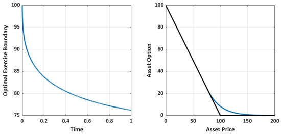
Figure 1.
Optimal exercise boundary and option value with order (1,2) predictor–corrector scheme (, ).
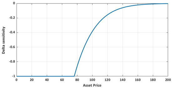
Figure 2.
Delta sensitivity with order (1,2) predictor–corrector scheme (, ).
Table 2.
Optimal exercise boundary with the predictor–corrector schemes (No. of grid interval , ).
Table 3.
Computational runtime(s) of the predictor–corrector schemes (No. of grid interval ).
In Figure 1 and Figure 2, we observe the smoothness in the numerical approximation of the optimal exercise boundary, option value, and delta sensitivity. Moreover, we observe that the results of order (1,2) and (2,2) predictor–corrector fourth-order compact finite difference schemes agree well with the result obtained from the method of Zhu and Zhang [6]. It is very important to observe from Table 2 and Table 3 that with small number of grid intervals (, ), the order (1,2) and (2,2) predictor–corrector fourth-order compact finite difference schemes provide a solution accuracy much closer to the result of the sixth-order compact finite difference up to 6-digit. Moreover, our (1,2) and (2,2) predictor–corrector schemes are very fast in computation even though our system of PDEs simultaneously solve the option value and delta sensitivity.
Here, it is worth mentioning that we define the runtime in seconds as the time required to run the whole code that approximates the option value, delta sensitivity, and the optimal exercise boundary simultaneously, excluding initialization and visualization. Initialization and visualization take insignificant computational runtime. However, it could be slightly significant here because we achieve reasonable accuracy with a very coarse grid and very little computational runtime. The main reason that enables the order (1,2) Euler-CN and (2,2) Leapfrog-CN predictor–corrector scheme to be very fast is the implementation of the Thomas algorithm in the three-iterative step of the corrector scheme.
To fully describe the computational speed we achieved with order (1,2) Euler-CN and (2,2) Leapfrog-CN predictor–corrector compact finite difference schemes, we computed the optimal exercise boundary, option value, and delta sensitivity simultaneously using a very small-time step with varying step sizes. We then compared the results with the one obtained from the sixth-order compact finite difference scheme. The numerical solution of the optimal exercise boundary and the computational runtime with these methods are listed in Table 4 and Table 5.
Table 4.
Computational runtime(s) and with and varying step sizes.
Table 5.
Optimal exercise boundary with and varying step sizes.
The importance of our order (1,2) and (2,2) predictor–corrector fourth-order compact finite difference schemes is that if we fix a very small-time step, as shown in Table 5, their computational runtime grows almost insignificantly and linearly as the step size in the space grid is exceedingly reduced. We observe this nice feature across all our numerical experiment with the above low-order (1,2) and (2,2) predictor–corrector fourth-order compact finite difference schemes. It is easy to further observe in Table 4 and Table 5 that both predictor–corrector schemes outperform the sixth-order compact scheme method in terms of computational runtime from . It is also interesting to see that when , the results of the (1,2) Euler-CN and (2,2) Leapfrog-CN predictor–corrector schemes are the same as that of the sixth-order compact scheme up to seven and eight digits even though our (1,2) and (2,2) PC schemes are implemented with a fourth-order compact scheme, signaling that our implementation shows a highly accurate result with a very little computational runtime. Moreover, the computational runtime for the sixth-order compact finite difference scheme is significantly high with a very refine space and time grid. Notwithstanding, we have already achieved seven-digit accuracy with the sixth-order compact finite difference method with and a runtime of 9 seconds, which is the main advantage of the sixth-order compact finite difference scheme over our (1,2) and (2,2) predictor–corrector schemes.
To better understand the importance of the three-step correction scheme we proposed based on the order (1,2) Euler-CN and order (2,2) Leapfrog-CN fourth-order compact finite difference scheme, we compared the computational results of the optimal exercise boundary based on one, two, three, and four iteration steps with the implicit scheme, as described in Table 6. From Table 6, we observe that as the number of iteration increases from 1 to 3, there is a substantial improvement in the solution accuracy. However, beyond a number of iterations of 3, the improvement in the solution accuracy is insignificant. Hence, there is no need to waste more computational effort, which is the reason why we use three iteration steps.
Table 6.
Optimal exercise boundary with different number of iterations using Euler-CN predictor–corrector compact scheme ().
In the second experiment, we compared the results of the option value and delta sensitivity with the existing methods. To this end, we considered the example in the work of Tangman et al. [24] with the parameter given in Table 7. For numerical comparison, we used a benchmark value obtained from the Binomial method with 15,001 steps [25]. We used a step size of and a time step of . The numerical results are listed in Table 8 and Table 9. For this example, we display the plot profiles for the (2,2) predictor–corrector fourth-order compact finite difference scheme in Figure 3 and Figure 4. The curves of the optimal exercise boundary, option value, and delta sensitivity admit sufficient smoothness. Moreover, we observe a close match between the result obtain from the low-order (1,2) and (2,2) predictor–corrector schemes as compared with the well-known methods, including the benchmark from the Binomial method [25].
Table 7.
Option parameters.
Table 8.
Option value with predictor–corrector schemes. WK is the method of Wu and Kwok [8]. OP is the operator splitting method [26]. BS1 and BS2 is the method of Brennan and Schwartz [27].
Table 9.
Delta sensitivity with predictor–corrector schemes. WK is the method of Wu and Kwok [8]. OP is the operator splitting method [26]. BS1 and BS2 is the method of Brennan and Schwartz [27].
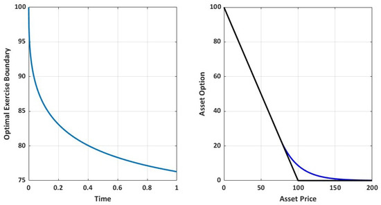
Figure 3.
Optimal exercise boundary and option value with order (2,2) predictor–corrector scheme (, ). = 76.284497.
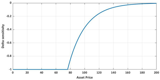
Figure 4.
Delta sensitivity with order (2,2) predictor–corrector scheme (, ).
In the last experiment, our interest was to compute the convergence rates of the present predictor–corrector schemes. To this end, we considered parameters in the second example. The only difference is that we used different time to maturity, given as . Here, we fixed the time step and then varied the step size, as shown in Table 10 and Table 11, where the maximum errors and convergence rate are displayed. The convergence rate results for the low-order (1,2) and (2,2) predictor–corrector schemes are reasonable. Moreover, further improvement can be achieved if the singularity associated with the first derivative of the optimal exercise boundary and inherent discontinuity associated with the model are carefully improved. In general, our proposed low-order (1,2) and (2,2) predictor–corrector fourth-order compact finite schemes which simultaneously solve the optimal exercise boundary, option value, and delta sensitivity are very fast and provide reasonable solution accuracy on both coarse and very refined grids.
Table 10.
Convergence rate result of the option value with (1,2) Euler-CN compact scheme.
Table 11.
Convergence rate result of the option value with (2,2) Leapfrog-CN compact scheme.
4.2. Order (3,3) and (4,4) Predictor–Corrector Schemes
Here, we investigate the performance of the presented (3,3) and (4,4) predictor–corrector integration methods with fourth-order compact finite difference scheme for solving the American option pricing model as a fixed free boundary problem. Consider the example in the work of Bunch and Johnson [28] with the following parameters displayed in Table 12.
Table 12.
Option parameters.
The benchmark solution as presented in the work of Bunch and Johnson [28] was obtained from the Binomial tree method with 10,000 steps. Our numerical approximations with this high-order predictor–corrector schemes are presented in Table 13 and Table 14. From Table 13 and Table 14, we observe reasonable solution accuracy across the high-order predictor–corrector schemes. Moreover, for the order (3,3) predictor–corrector fourth-order compact finite difference schemes, we observe that the BDF3 scheme has the lowest accuracy and - has the best accuracy as compared with the benchmark value. For the (4,4) predictor–corrector scheme, - performed better than -BDF4. However, the discrepancy in results among the high-order predictor–corrector compact finite difference schemes is not substantial. Finally, we plotted the curves of the optimal exercise boundary, option value, and delta sensitivity obtained from the - predictor–corrector fourth-order compact finite difference schemes in Figure 5, Figure 6 and Figure 7.
Table 13.
Option value with the (3,3) and(4,4) predictor–corrector schemes (). The benchmark value is the Binomial method (BM) with 10,000 steps.
Table 14.
Delta sensitivity with the (3,3) and (4,4) predictor–corrector schemes (). The benchmark value is the Binomial method (BM) with 10,000 steps.
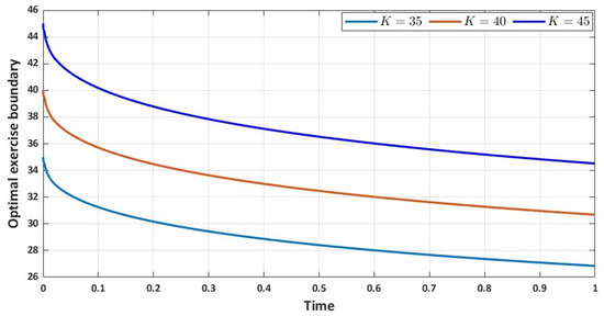
Figure 5.
Optimal exercise boundary with - and varying strike price.
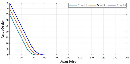
Figure 6.
Option value with - and varying strike price.
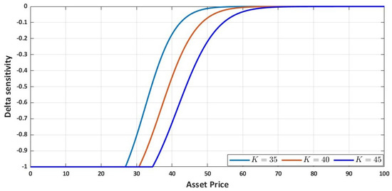
Figure 7.
Delta sensitivity with - and varying strike price.
5. Conclusions
We have explored the efficiency of a suite of predictor–corrector schemes with fourth-order compact finite difference for solving a system of American option pricing PDEs consisting of the option value and delta sensitivity as a free boundary problem. The numerical results shows that the low-order (1,2) Euler-CN and (2,2) Leapfrog-CN predictor–corrector compact finite difference schemes have great performance in terms of computational speed and accuracy. Moreover, (1,2) Euler-CN and (2,2) Leapfrog-CN are very fast in both coarse and very refined grids and also present highly accurate solutions with coarse grids and little computation runtime. This is largely possible due to the implementation of the Thomas algorithm and fourth-order compact finite difference schemes. Moreover, the speed of our computation is further enhanced by using only three iterative steps at each time-level with the second-order CN and fourth-order compact finite difference correction schemes. We also obtain reasonable convergence rate results with these two implementations. For extension purposes, we have further explored the suite of high-order predictor–corrector schemes and have obtained reasonable solution accuracy. In general, we can validate that our implementations are very efficient and could be extendable to solving other free boundary option pricing problems.
In our future work, we hope to further enhance the performance of our proposed suite of low- and high-order predictor–corrector fourth-order compact finite difference schemes by improving the smoothness and irregularity inherent in the transformed model such that we can recover numerical convergence rate that is consistently in good agreement with the theoretical one. Furthermore, we hope in our future work to extend this method and its variants to non-standard and exotic options including stochastic volatility models.
Author Contributions
Conceptualization, C.N. and W.D.; methodology, C.N.; software, C.N.; validation, C.N.; formal analysis, C.N.; investigation, C.N.; resources, C.N.; data curation, C.N.; writing—original draft preparation, C.N.; writing—review and editing, W.D.; visualization, C.N.; supervision, W.D.; project administration, W.D. All authors have read and agreed to the published version of the manuscript.
Funding
This research received no external funding.
Data Availability Statement
Not applicable.
Acknowledgments
The first author is funded in part by an NSERC Discovery Grant.
Conflicts of Interest
The authors declare no conflict of interest.
References
- Kazmi, K. An IMEX predictor–corrector method for pricing options under regime-switching jump-diffusion models. Int. J. Comput. Math. 2019, 96, 1137–1157. [Google Scholar] [CrossRef]
- Kalantari, R.; Shahmorad, S.; Ahmadian, D. The stability analysis of predictor–corrector method in solving American option pricing model. Comput. Econ. 2016, 47, 255–274. [Google Scholar] [CrossRef]
- Khaliq, A.Q.M.; Voss, D.A.; Kazmi, S.H.K. A linearly implicit predictor–corrector scheme for pricing American options using a penalty method approach. J. Bank. Financ. 2006, 30, 489–502. [Google Scholar] [CrossRef]
- Chen, W.; Xu, X.; Zhu, S.P. A predictor–corrector approach for pricing American options under the finite moment log-stable model. Appl. Numer. Math. 2015, 97, 15–29. [Google Scholar] [CrossRef]
- Hajipour, M.; Malek, A. Efficient high-order numerical methods for pricing of options. Comput. Econ. 2015, 45, 31–47. [Google Scholar] [CrossRef]
- Zhu, S.P.; Zhang, J. A new predictor–corrector scheme for valuing American puts. Appl. Math. Comput. 2011, 217, 4439–4452. [Google Scholar] [CrossRef]
- Zhu, S.P.; Chen, W.T. A predictor–corrector scheme based on the ADI method for pricing American puts with stochastic volatility. Comput. Math. Appl. 2011, 62, 1–26. [Google Scholar] [CrossRef]
- Wu, L.; Kwok, Y.K. A front-fixing finite difference method for the valuation of American options. J. Financ. Eng. 1997, 6, 83–97. [Google Scholar]
- Zhao, J.; Corless, R.M. Compact finite difference method for integro-differential equations. Appl. Math. Comput. 2006, 177, 271–288. [Google Scholar] [CrossRef]
- Zhao, J. Highly accurate compact mixed methods for two point boundary value problems. Appl. Math. Comput. 2007, 188, 1402–1418. [Google Scholar] [CrossRef]
- Zhao, J.; Davison, M.; Corless, R.M. Compact finite difference method for American option pricing. J. Comput. Appl. Math. 2007, 206, 306–321. [Google Scholar] [CrossRef]
- Egorova, V.N.; Jódar, L. Solving American option pricing models by the front fixing method: Numerical analysis and computing. In Abstract and Applied Analysis; Hindawi: London, UK, 2014; Volume 2014. [Google Scholar]
- Egorova, V.N.; Company, R.; Jódar, L. A new efficient numerical method for solving American option under regime switching model. Comput. Math. Appl. 2016, 71, 224–237. [Google Scholar] [CrossRef]
- Kwok, Y.K. Mathematical Models of Financial Derivatives; Springer: Berlin/Heidelberg, Germany, 2008. [Google Scholar]
- Musiela, M.; Rutkowski, M. Martingale Methods in Financial Modelling; Springer Science & Business Media: Berlin/Heidelberg, Germany, 2006. [Google Scholar]
- Zhang, K.; Song, H.; Li, J. Front-fixing FEMs for the pricing of American options based on a PML technique. Appl. Anal. 2015, 94, 903–931. [Google Scholar] [CrossRef]
- Adam, Y. A Hermitian finite difference method for the solution of parabolic equations. Comput. Math. Appl. 1975, 1, 393–406. [Google Scholar] [CrossRef]
- Adam, Y. Highly accurate compact implicit methods and boundary conditions. J. Comput. Phys. 1977, 24, 10–22. [Google Scholar] [CrossRef]
- Carpenter, M.H.; Gottlieb, D.; Abarbanel, S. The stability of numerical boundary treatments for compact high-order finite-difference schemes. J. Comput. Phys. 1993, 108, 272–295. [Google Scholar] [CrossRef]
- Carpenter, M.H.; Gottlieb, D.; Abarbanel, S. Stable and accurate boundary treatments for compact, high-order finite-difference schemes. Appl. Numer. Math. 1993, 12, 55–87. [Google Scholar] [CrossRef]
- Abrahamsen, D.; Fornberg, B. Solving the Korteweg-de Vries equation with Hermite-based finite differences. Appl. Math. Comput. 2021, 401, 126101. [Google Scholar] [CrossRef]
- Li, M.; Tang, T. A compact fourth-order finite difference scheme for unsteady viscous incompressible flows. J. Sci. Comput. 2001, 16, 29–45. [Google Scholar] [CrossRef]
- Nwankwo, C.; Dai, W. Sixth-order compact differencing with staggered boundary schemes and 3(2) Bogacki-Shampine pairs for pricing free-boundary options. arXiv 2022, arXiv:2207.14379. [Google Scholar]
- Tangman, D.Y.; Gopaul, A.; Bhuruth, M. A fast high-order finite difference algorithm for pricing American options. J. Comput. Appl. Math. 2008, 222, 17–29. [Google Scholar] [CrossRef]
- Leisen, D.P.; Reimer, M. Binomial models for option valuation-examining and improving convergence. Appl. Math. Financ. 1996, 3, 319–346. [Google Scholar] [CrossRef]
- Ikonen, S.; Toivanen, J. Operator splitting methods for American option pricing. Appl. Math. Lett. 2004, 17, 809–814. [Google Scholar] [CrossRef]
- Brennan, M.J.; Schwartz, E.S. The valuation of American put options. J. Financ. 1977, 32, 449–462. [Google Scholar] [CrossRef]
- Bunch, D.S.; Johnson, H. The American put option and its critical stock price. J. Financ. 2000, 55, 2333–2356. [Google Scholar] [CrossRef]


Disclaimer/Publisher’s Note: The statements, opinions and data contained in all publications are solely those of the individual author(s) and contributor(s) and not of MDPI and/or the editor(s). MDPI and/or the editor(s) disclaim responsibility for any injury to people or property resulting from any ideas, methods, instructions or products referred to in the content. |
© 2023 by the authors. Licensee MDPI, Basel, Switzerland. This article is an open access article distributed under the terms and conditions of the Creative Commons Attribution (CC BY) license (https://creativecommons.org/licenses/by/4.0/).