Abstract
This paper proposes a new time-varying integer-valued autoregressive (TV-INAR) model with a state vector following a logistic regression structure. Since the autoregressive coefficient in the model is time-dependent, the Kalman-smoothed method is applicable. Some statistical properties of the model are established. To estimate the parameters of the model, a two-step estimation method is proposed. In the first step, the Kalman-smoothed estimation method, which is suitable for handling time-dependent systems and nonstationary stochastic processes, is utilized to estimate the time-varying parameters. In the second step, conditional least squares is used to estimate the parameter in the error term. This proposed method allows estimating the parameters in the nonlinear model and deriving the analytical solutions. The performance of the estimation method is evaluated through simulation studies. The model is then validated using actual time series data.
Keywords:
time-varying integer-valued autoregressive model; parameter estimation; Kalman-smoother; logistic regression; conditional least squares MSC:
62M10
1. Introduction
Time series models with an integer-valued structure are prevalent in fields such as economics, insurance, medicine and crime. Recent reviews on count time series models based on thinning operators, including modeling and numerous examples, can be found in refs. [1,2,3]. The most classic one is the first-order integer-valued autoregressive INAR(1) model introduced by ref. [4] and ref. [5] using the properties of binomial sparse operators (ref. [6]). The class of INAR models is typically based on the assumption of observations that follow a Poisson distribution, which facilitates subsequent computations due to the equidispersion feature of the Poisson distribution (mean and variance being equal). Parameter estimation for these models is usually achieved by Yule–Walker, conditional least squares and conditional maximum likelihood methods, as discussed in refs. [7,8,9], among others. Recently, there has been a growing interest in research regarding the autoregressive coefficients in these models. Generally, the autoregressive coefficients can be treated as random variables, with rules such as a stationary process or specified mean and variance; see refs. [10,11,12]. Unlike the above models, this paper proposes a time-varying integer-valued autoregressive (TV-INAR) model in which the state equation is a nonstationary form.
In our work, the model is characterized by a state equation and time-varying parameters. The concept of state-space time series analysis was first introduced by ref. [13] in the field of engineering. Over time, the term “state space” became entrenched in statistics and econometrics, as the state-space model provides an effective method to deal with a wide range of problems in time series analysis. Ref. [14] presented a comprehensive treatment of the state-space approach to time series analysis. Recently, some progress has been made on the use of state space in integer autoregressive and count time series models. Ref. [15] proposed a first-order random coefficient integer-valued autoregressive model by introducing a Markov chain with a finite state space and derived some statistical properties of the model in a random environment. Ref. [16] introduced a parameter-driven state-space model to analyze integer-valued time series data. And, to accommodate the features of overdispersion, zero-inflation and temporal correlation of count time series, ref. [17] proposed a flexible class of dynamic models in the state-space framework. As noted in ref. [18], the popularity of these models stems in large part from the development of the Kalman recursion, proving a quick updating scheme for predicting, filtering and smoothing a time series. The traditional understanding of Kalman filtering can be found in the works of refs. [14,19,20]. Nevertheless, most of this research has focused on the use of continuous time series models in an economic context, such as the analysis of stocks, trade and currency. For example, ref. [21] proposed a class of time-varying parameter autoregressive models and proved the equivalence of the Kalman-smoothed estimate and generalized least squares estimate. Following this lead, [22] developed a trade growth relationship model with time-varying parameters and estimated the transition of changing parameters with a Kalman filter. Both of them all involved cases of Gaussian and linear parameters. Ref. [14] attested that the results obtained by Kalman smoothing are equivalent when the model is non-Gaussian or nonlinear. Therefore, integer-valued time series models in the non-Gaussian case are also worth investigating.
Time series models with state-space and time-varying parameters are common in economics. Many macroeconomists believe that time-varying parameter models can better predict and adapt to the data than fixed-parameter models. Early research mostly focused on time-varying continuous time series models, such as the autoregressive (AR) models, vector autoregressive (VAR) models and autoregressive moving average (ARMA) models (see refs. [21,23,24]). In recent years, research on INAR models with time-varying parameters has attracted more attention and has been applied to natural disasters and medical treatment. Ref. [25] introduced a multivariate integer-valued autoregressive model of order one with periodic time-varying parameters and adopted a composite likelihood-based approach. Ref. [26] considered a change-point analysis of counting time series data through a Poisson INAR(1) process with time-varying smoothing covariates. However, the time-varying parameters in the above models are not controlled by a state equation. Additionally, it is difficult to deal with time-varying parameter models when there are unobserved variables that need to be estimated. There are only a few effective methods available. Ref. [27] proposed a Bayesian estimation method for time-varying parameters and claimed that the Bayesian method is superior to the maximum likelihood method. Both the Bayesian and maximum likelihood methods require Kalman filtering to estimate state vectors that contain time-varying parameters. The application of the Kalman filter would be made possible once the model is put into a state-space form. It is worth exploring some new methods to deal with TV-INAR models.
Motivated by ref. [21], a new TV-INAR model with a state equation is presented in this paper. Since the model is in a state-space form, the Kalman smoothing method uses only known observation variables to estimate the parameters. Unlike traditional INAR models, which are limited to modeling stationary time series data, our TV-INAR model is equipped to handle nonstationary structures and time-varying dynamics, resulting in improved model fit and more accurate predictions. The Kalman-smoothed estimates of the time-varying unobserved state variables are derived. Furthermore, the mean of the Poisson error term is estimated through the estimates obtained in the previous step and conditional least squares methods.
The rest of this paper is organized as follows. A new TV-INAR model is presented and its basic properties are constructed in Section 2. In Section 3, the Kalman smoother is utilized to derive an estimate of the time-varying parameter. Then, incorporating conditional least squares (CLS) methods, the estimation of the mean of the Poisson error term is established. Numerical simulations and results are discussed in Section 4. In Section 5, the proposed model is applied to the offense data sets in Rochester. The conclusion is given in Section 6.
2. Poisson TV-INAR Model
In this section, the INAR(1) model is reviewed. A new TV-INAR model incorporating time-varying and nonstationary features is introduced. Then, some basic statistical properties are derived.
Suppose Y is a non-negative integer-valued random variable and . The binomial thinning ∘, introduced in ref. [6], is defined as , where is a sequence of independent and identically distributed (i.i.d.) Bernoulli random variables, independent of Y, and satisfying . Then, the INAR(1) model is given by
where is a sequence of uncorrelated non-negative integer-valued random variables, with mean and finite variance , and is independent of all .
2.1. Definition of TV-INAR Process
It is very common to extend the autoregressive coefficient to a random parameter in time series models. However, it differs from the time-varying parameter introduced in this paper. In random coefficient (RC) models, the variable is usually assigned a definite distribution or given its expectation and variance. Although it is a random variable, its expectation and variance do not change with time. In contrast, in time-varying parameter models, the parameter does not have a fixed distribution, and its expectation and variance often change over time. This is also one of the challenges of such models compared with the ordinary RC models. Thus, based on the above INAR(1) process, we define the time-varying integer-valued autoregressive (TV-INAR) process as follows.
Definition 1.
Let be an integer-valued regressive process. It is a time-varying integer-valued regressive model if
where is a function of ; is a sequence of i.i.d. Poisson-distributed random variables with mean λ; is a sequence of i.i.d. standard normally distributed random variables; and is independent of and when .
In the model (2), and are observation variables, and is an unobserved variable, often called a time-varying parameter. Our model allows the class of TV-INAR models. For example, yields a TV-INAR(1) model. Model (2) becomes a TV-INAR(p) model when and the autocorrelation coefficient expands to . Furthermore, can also be considered as a covariate of .
In this paper, we devote the case of . The idea of this model is that the development of the system over time is determined by in the second equation of (2). However, since cannot be observed directly, we need to analyze it based on the observations . The first equation of (2) is called the observation equation; the second is called the state equation [14]. We assume initially that where and are known, because the state equation is nonstationary. Variances of the error terms and in (2) are time-invariant.
Studies on the class of TV-AR models have been extensive, especially in the field of economics. Such models are flexible enough to capture the complexity of macroeconomic systems and fit the data better than models with constant parameters. Retaining the advantages of the above models, we propose the TV-INAR model, which can deal with integer-valued discrete data and exists in real life. And, it is of interest that is always nonstationary, as is a random walk. Therefore, the existence of the above state equation is justified. And the binomial thinning operator ∘ portrays the probability of the event, so is given the form to ensure that the probability is between (0,1).
2.2. Statistical Properties
To have a better understanding of the model and to apply it directly to parameter estimation, some statistical properties of the model are provided. The mean, conditional mean, second-order conditional origin moment, variance and conditional variance of the time-varying integer-valued regressive process are given in the following proposition. The case of TV-INAR(1) is given in the corollary.
Proposition 1.
Suppose is a process defined by (2), and is a σ-field generated by . Then, when , we have
- (1)
- (2)
- (3)
Corollary 1.
Suppose satisfies the TV-INAR(1) model, i.e., , and , then for ,
- (1)
- (2)
- (3)
- (4)
Clearly, when , is a bivariate Markov chain with the following transition probabilities:
3. Estimation Procedure
There are two interesting parameters in the model, one is the time-varying parameter , and the other is the mean of . The main goal of this section is to estimate these two parameters using a new two-step estimation method. The first step gives the estimate by Kalman-smoothed state. In the second step, the estimate is obtained by and the conditional least squares (CLS) method.
3.1. Kalman-Smoothed Estimate of State Vector
In this subsection, the Kalman-smoothed method is used to estimate the time-varying parameter. In fact, the essence of the Kalman filter is the minimum variance linear unbiased estimation (MVLUE). From ref. [14], we know that when the model is nonlinear and non-Gaussian, the results obtained from the standpoint of MVLUE are equivalent to the linear and Gaussian cases. To find the Kalman-smoothed estimate of the unobserved state vector, we employ the matrix formulation of Equation (2) following ref. [14]. The required moments are calculated and the analytic expression of this estimate is given at the end.
For convenience, set . Then, is a logistic transformation. For , Equation (2) can be written in matrix form, similarly to ref. [21]:
where
Now, consider the problem of estimating the parameter. The following theorem adapted from ref. [14] provides the Kalman-smoothed estimate of the state vector in model (3).
Theorem 1.
The Kalman-smoothed estimate of in model (3) is given by the conditional expectation of , which contains all the observations of :
Proof.
Let , where is a vector , B is a vector and A is a matrix . Denote
This is the error covariance matrix of state vector estimation, and it can be regarded as a function on A and B. To minimize I, we need
We obtain
This proves that □
Theorem 1 contains some numerical characteristics of the random variable. Following model (3), we denote . Then, the mean of and , the variance of and the covariance between and are given in the following proposition.
Proposition 2.
Suppose is a TV-INAR process defined by (3). Then, for any time T,
- (i)
- ;
- (ii)
- ;
- (iii)
- (iv)
- .
The proofs of Proposition 2 are given in Appendix A. From Proposition 2, the Kalman-smoothed estimate of the time-varying parameter is
where and are random variables. Hence, in order to obtain the concrete result of the estimate, we need to compute the numerical characteristics of the random variables in Equation (5), i.e., and , where denote instances in time.
First, we set . Then, we have
Here, stands for the logarithmic Normal distribution. Denote X as , as its mean and as its variance, respectively. Then, , and the probability density function of X is
Similarly, denote Y as and as its variance, respectively. Then, . According to the logistic transformation, . So can be expressed in terms of X, i.e., . Thus, from the distributions of X and Y, the following proposition can be established.
Proposition 3.
Suppose and are elements of in Proposition 2, and is an element of . Denote
Then, for any ,
- (1)
- (2)
- (3)
- (4)
- When ,When ,
- (5)
The proofs of Proposition 3 are given in Appendix B. And the distribution function of the standard normal distribution and Taylor’s formula are used. Clearly, the exact solution of the time-varying parameter is found by substituting (1)–(5) of Proposition 3 into Equation (5). Since , if r tends to infinity, all of the in Proposition 3 converge to 0. The corresponding results are specified in Remark 1.
Remark 1.
The items involving in Proposition 3 can be divided into two categories, namely and , where a and b are constants greater than 0. According to the properties of the distribution function of the standard normal distribution, if r tends to infinity, the following limits apply:
Therefore, (1)–(5) in Proposition 3 are convergent. Moreover, the Kalman-smoothed estimate in (5) is also convergent.
3.2. CLS Estimation of Parameter
Based on the proposed TV-INAR model and its statistical properties, we consider the parameter estimation problem on in the model. Here, the estimate obtained in the previous section is used directly. Due to the characteristics of the model, that is, the state equation is nonstationary, the autoregressive coefficient in the observation equation is time-varying and the distribution is unknown, many estimation methods are not suitable for this model. Considering that the CLS estimation method does not need the distribution hypothesis of the model but only the corresponding moment information, and the estimation accuracy is relatively high, we prefer using the CLS method to estimate .
Suppose there is a TV-INAR process . Let
be the CLS criterion function. Then, the CLS estimator of the parameter can be obtained by minimizing the CLS criterion function, i.e.,
Taking the derivative of with respect to and setting it to zero, the minimizer can be found:
This is the CLS estimate of .
4. Simulation
In this section, we perform simulations using Matlab R2018b to assess the performance of the two-step estimation approach discussed in Section 3. The approach recovers the true time-varying parameters, as well as the performance of the CLS estimator.
For the data generating process, using Equation (3), pseudodata are randomly generated by changing time T () and the parameter () of the error term in the observation equation. The number of replications was 100. Here, the choice of is based on the size of the signal-to-noise ratio (SNR), which is defined as the variance in relative to that in , i.e., SNR . In our model, the error of the state equation is constant. So, we consider the SNRs for 1/0.05, 1/0.1, 1/0.8, 1/1.3 and 1/4 by changing the variance in the error () in the observation equation. And these five sample paths of the TV-INAR(1) model are plotted in Figure 1, respectively. We can see that the sample path of is unsteady, and the variation in parameter combinations results in a change in the sample dispersion of the samples.
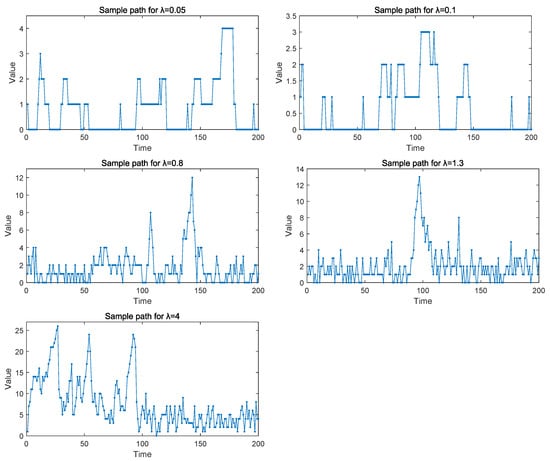
Figure 1.
Sample paths of the TV-INAR(1) model for .
Then, we should notice the choice of the parameter’s initial value. The initial value of follows a known normal distribution, which is mentioned in Section 2.1. In practice, it is difficult to gauge the true value of its mean and the variance of the distribution. For simplicity, we assume is known and nonstochastic, i.e., . This assumption brings great convenience in simulation studies and does not affect numerical results. This can be observed in Proposition 3 when the sample size is sufficiently large.
Our simulation concerns a first-order integer-valued autoregressive model with time-varying parameters (TV-INAR(1)). For the first step estimation, let denote the true value of the parameter in the data generation process and denote the Kalman-smoothed estimate of the parameter. We compute the sample means and sample standard deviations of the true and estimated values, respectively:
After replications, the averages of the above four indicators are found, respectively:
Let . We take the difference between and directly to evaluate the effectiveness of the Kalman-smoothed estimate approach. In addition, denote
as the mean of the ratio of the standard deviation of to the standard deviation of the real process . The quality of the estimator depends on whether is close to one. This is similar to the criterion in [21].
Next, we evaluate the performance of the second step estimation, which is to apply the and the conditional least squares (CLS) method to estimate the parameter in the model (2). As we mentioned above, the true value of is considered . To evaluate the estimation performance, besides considering , two other indicators were selected, which are the mean absolute deviation (MAD) and mean square error (MSE), as defined below:
where is the estimation result of at the nth replication. Then, considering various sample sizes and initial parameter values, the simulation results of the two-step estimation process are listed in Table 1 and Table 2.

Table 1.
Simulation results of .
Table 2.
Simulation results of .
It is shown that the smaller the variance () of the error term, the smaller the biases of estimates and . This implies that the Kalman smoothing and CLS approaches work better in the sense of . In the first-step estimation, the larger the variance (), the closer is to one. In this sense, the Kalman smoothing method is the best if is equal to 1.3. This suggests that only using one criterion to measure the effectiveness of the estimation method is insufficient. In addition, by increasing the sample size, is smaller and is closer to one. This shows that the Kalman-smoothed estimate is closer to the true process. From the perspective of SNR, the larger the SNR, the smaller the bias in the estimation. The smaller the SNR, the closer the estimated median sample variance is to the true process. In summary, when the SNR is around 1, the estimation is relatively good. In the second-step estimation, the values of MAD and MSE are small, suggesting a relatively acceptable estimation effect. The estimation results as a whole show a trend that the larger the SNR, the smaller the estimation error. Consequently, the CLS estimate method works better. Additionally, when the sample size T increases, the corresponding MAD and MSE gradually decrease, and the estimates of the parameter gradually converge to the true values. In conclusion, the proposed two-step estimation method is a credible approach.
5. Case Application
In this section, we apply the model and method of Section 3 to predict real-time series data. The data set is a count time series of offense data, obtainable from the NSW Bureau of Crime Statistics and Research covering January 2000 to December 2009. The observations represent monthly counts of Sexual offenses in Ballina, NSW, Australia, which comprise 120 monthly observations. Figure 2 shows the time plot and partial autocorrelation function (PACF). It shows that the data are nonstationary and are first-order autocorrelated, which is an indication that it could be reasonable to model this data set with our model. The descriptive statistics of the data are displayed in Table 3. Next, we compared our TV-INAR(1) model with the INAR(1) model to fit the data set. In general, it is expected that the better model to fit the data presents smaller values for -log-likelihood, AIC and BIC. From the results in Table 4, we can conclude that the proposed model fits the data better.
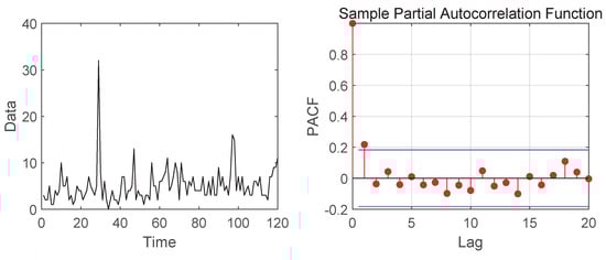
Figure 2.
Time plot and PACF of sexual offense data for the period 2000−2009.
Table 3.
Descriptive statistics for sexual offense data.
Table 4.
Estimates of the parameters and goodness-of-fit statistics for the offense data.
For the prediction, the predicted values of the offense data are given by
Specifically, the one-step-ahead conditional expectation point predictor is given by
We compute the root mean square of the prediction errors (RMSEs) of the data in the past 6 months, with the RMSE defined as
The estimators and RMSE results are also shown in Table 4. To analyze the adequacy of the model, we analyze the standardized Pearson residuals, defined as
with . For our model, the mean and variance of the Pearson residuals are 0.8022 and 1.2000, respectively. As discussed in ref. [28], for an adequately chosen model, the variance of the residuals should take a value close to 1. And 1.2 seems to be close to 1. Therefore, we conclude that the proposed model fits the data well.
6. Conclusions
This paper proposes a time-varying integer-valued autoregressive model with autoregressive coefficients driven by a logistic regression structure. It can be more flexible and efficient to handle integer-valued discrete and even nonstationary data. Some statistical properties of the model are derived, such as mean, variance, covariance, conditional mean and conditional variance. A two-step estimation method was introduced. Since the model is in a state-space form, the Kalman smoothing method would instead be used to estimate the time-varying parameter. In the first step, the Kalman-smoothed estimate of the state vector is obtained using the information of the known observation variables. In the second step, the estimate from the previous step and the CLS method are used to obtain the estimate of the error term parameter. The analysis formulae of the estimates in the two steps are both derived. The solution challenge lies in calculating the covariance matrix and the correlation between the variables. The advantage of this method is that the approximate estimation of the unknown parameters can be obtained from all the observable variables, and the approach has superior performance in practical applications, even in the case of nonlinear and non-Gaussian errors. The proposed method can also estimate the time-varying parameters well. In addition, an application of forecasting a real data set is presented. The results suggest that the TV-INAR(1) model is more suitable for practical data sets. In model (3), if the variances of the error terms and are allowed to be time-dependent, the model will be regarded as a stochastic volatility model. This is a topic for discussion. Moreover, extending the research outcomes to the p-order model TV-INAR(p) is one direction of future research.
Author Contributions
Every author contributed equally to the development of this paper. Conceptualization, D.W.; ethodology, Y.P.; software, Y.P.; investigation, Y.P.; writing—original draft preparation, Y.P.; writing—review and editing, D.W. and M.G.; supervision, D.W. and M.G.; funding acquisition, D.W. All authors have read and agreed to the published version of the manuscript.
Funding
This research was funded by the National Natural Science Foundation of China (Nos. 12271231, 12001229, 11901053).
Data Availability Statement
Publicly available data sets were analyzed in this study. These data can be found here: [https://data.nsw.gov.au/data/dataset/nsw-criminal-court-statistics] (accessed on 3 July 2023).
Conflicts of Interest
The authors declare no conflicts of interest.
Appendix A. Proof of Proposition 2
- (i)
- ;
- (ii)
- ;
- (iii)
- (iv)
- .
For any
Thus, .
Appendix B. Proof of Proposition 3
(1) . Denote . Using substitution and Taylor’s expansion, we obtain
Then,
(2) ,
Then,
(3)
(4)
where and they are independent of each other. The same applies when . Let Y denote and denote its variance. Thus, .
When ,
where
Thus,
Similarly, when ,
X and Y are independent, and . Therefore,
(5) According to the state equation in (2),
Let X denote and Y denote . Then, . For convenience, let and represent the mean and variance of X in the computation. Thus,
where can be obtained from (A1).
Therefore,
References
- Karlis, D.; Khan, N.M. Models for integer data. Annu. Rev. Stat. Appl. 2023, 10, 297–323. [Google Scholar] [CrossRef]
- Scotto, M.G.; Weiß, C.H.; Gouveia, S. Thinning-based models in the analysis of integer-valued time series: A review. Stat. Model. 2015, 15, 590–618. [Google Scholar] [CrossRef]
- Weiß, C.H. An Introduction to Discrete-Valued Time Series; John Wiley and Sons, Inc.: Chichester, UK, 2018. [Google Scholar]
- McKenzie, E. Some simple models for discrete variate time series. Water Resour. Bull. 1985, 21, 645–650. [Google Scholar] [CrossRef]
- Al-Osh, M.A.; Alzaid, A.A. First-order integer-valued autoregressive (INAR(1)) process. J. Time Ser. Anal. 1987, 8, 261–275. [Google Scholar] [CrossRef]
- Steutel, F.W.; Van, H.K. Discrete analogues of self-decomposability and stability. Ann. Probab. 1979, 7, 893–899. [Google Scholar] [CrossRef]
- Freeland, R.K.; McCabe, B. Analysis of low count time series data by Poisson autoregression. J. Time Ser. Anal. 2004, 25, 701–722. [Google Scholar] [CrossRef]
- Freeland, R.K.; McCabe, B. Asymptotic properties of CLS estimators in the Poisson AR(1) model. Stat. Probab. Lett. 2005, 73, 147–153. [Google Scholar] [CrossRef]
- Yu, M.; Wang, D.; Yang, K.; Liu, Y. Bivariate first-order random coefficient integer-valued autoregressive processes. J. Stat. Plan. Inference 2020, 204, 153–176. [Google Scholar] [CrossRef]
- Deng, Z.L.; Gao, Y.; Mao, L.; Li, Y.; Hao, G. New approach to information fusion steady-state Kalman filtering. Automatica 2005, 41, 1695–1707. [Google Scholar] [CrossRef]
- Sbrana, G.; Silvestrini, A. Random coefficient state-space model: Estimation and performance in M3-M4 competitions. Int. J. Forecast. 2022, 38, 352–366. [Google Scholar] [CrossRef]
- You, J.; Chen, G. Parameter estimation in a partly linear regression model with random coefficient autoregressive errors. Commun. Stat. Theory Methods 2022, 31, 1137–1158. [Google Scholar] [CrossRef]
- Kalman, R.E. A new approach to linear filtering and prediction problems. J. Fluids Eng. 1960, 82, 35–45. [Google Scholar] [CrossRef]
- Durbin, J.; Koopman, S.J. Time Series Analysis by State Space Methods. In Oxford Statistical Science Series, 2nd ed.; Oxford University Press: Oxford, UK, 2012. [Google Scholar]
- Tang, M.T.; Wang, Y.Y. Asymptotic behavior of random coefficient INAR model under random environment defined by difference equation. Adv. Differ. Equ. 2014, 1, 99. [Google Scholar] [CrossRef]
- Koh, Y.B.; Bukhari, N.A.; Mohamed, I. Parameter-driven state-space model for integer-valued time series with application. J. Stat. Comput. Simul. 2019, 89, 1394–1409. [Google Scholar] [CrossRef]
- Yang, M.; Cavanaugh, J.E.; Zamba, G.K.D. State-space models for count time series with excess zeros. Stat. Model. 2015, 15, 70–90. [Google Scholar] [CrossRef]
- Davis, R.A.; Dunsmuir, W.T.M. State space models for count time series. In Handbook of Discrete-Valued Time Series; Davis, R., Holan, S., Lund, R., Ravishanker, N., Eds.; CRC Press: Boca Raton, FL, USA, 2016; pp. 121–144. [Google Scholar]
- Duncan, D.B.; Horn, S.D. Linear dynamic recursive estimation from the viewpoint of regression analysis. J. Am. Stat. Assoc. 1972, 67, 815–821. [Google Scholar] [CrossRef]
- Maddala, G.S.; Kim, I. Unit Roots, Cointegration, and Structural Change; Cambridge University Press: Cambridge, UK, 1998. [Google Scholar]
- Ito, M.; Noda, A.; Wada, T. An Alternative Estimation Method for Time-Varying Parameter Models. Econometrics 2022, 10, 23. [Google Scholar] [CrossRef]
- Omorogbe, J.A. Kalman filter and structural change revisited: An application to foreign trade-economic growth nexus. Struct. Chang. Econom. Model. 2019, 808, 49–62. [Google Scholar]
- Bernanke, B.S.; Mihov, I. Measuring monetary policy. Q. J. Econ. 1998, 113, 869–902. [Google Scholar] [CrossRef]
- Ito, M.; Noda, A.; Wada, T. International stock market efficiency: A non-Bayesian time-varying model approach. Appl. Econ. 2014, 46, 2744–2754. [Google Scholar] [CrossRef]
- Santos, C.; Pereir, I.; Scotto, M.G. On the theory of periodic multivariate INAR processes. Stat. Pap. 2021, 62, 1291–1348. [Google Scholar] [CrossRef]
- Chattopadhyay, S.; Maiti, R.; Das, S.; Biswas, A. Change-point analysis through INAR process with application to some COVID-19 data. Stat. Neerl. 2022, 76, 4–34. [Google Scholar] [CrossRef] [PubMed]
- Primiceri, G.E. Time varying structural vector autoregressions and monetary policy. Rev. Econ. Stud. 2005, 72, 821–852. [Google Scholar] [CrossRef]
- Aleksandrov, B.; Weiß, C.H. Testing the dispersion structure of count time series using Pearson residuals. AStA Adv. Stat. Anal. 2019, 104, 325–361. [Google Scholar] [CrossRef]

Disclaimer/Publisher’s Note: The statements, opinions and data contained in all publications are solely those of the individual author(s) and contributor(s) and not of MDPI and/or the editor(s). MDPI and/or the editor(s) disclaim responsibility for any injury to people or property resulting from any ideas, methods, instructions or products referred to in the content. |
© 2023 by the authors. Licensee MDPI, Basel, Switzerland. This article is an open access article distributed under the terms and conditions of the Creative Commons Attribution (CC BY) license (https://creativecommons.org/licenses/by/4.0/).