A Three-Block Inexact Heterogeneous Alternating Direction Method of Multipliers for Elliptic PDE-Constrained Optimization Problems with a Control Gradient Penalty Term

Abstract

Optimization problems with PDE constraints are widely used in engineering and technical fields. In some practical applications, it is necessary to smooth the control variables and suppress their large fluctuations, especially at the boundary. Therefore, we propose an elliptic PDE-constrained optimization model with a control gradient penalty term. However, introducing this penalty term increases the complexity and difficulty of the problems. To solve the problems numerically, we adopt the strategy of “First discretize, then optimize”. First, the finite element method is employed to discretize the optimization problems. Then, a heterogeneous strategy is introduced to formulate the augmented Lagrangian function for the subproblems. Subsequently, we propose a three-block inexact heterogeneous alternating direction method of multipliers (three-block ihADMM). Theoretically, we provide a global convergence analysis of the three-block ihADMM algorithm and discuss the iteration complexity results. Numerical results are provided to demonstrate the efficiency of the proposed algorithm.

1. Introduction

Elliptic PDE-constrained optimization problems are of significant importance in many fields, including engineering, physics, biology and finance. In engineering, they are essential for optimizing designs in structural mechanics, fluid dynamics, and electromagnetics. In physics, they are crucial to modeling heat transfer, quantum mechanics, and elasticity. In biology, these problems are integral in utilizing modeling diffusion processes, population dynamics, and biochemical reactions. Furthermore, in finance, they are vital for option pricing, risk management, and portfolio optimization. The versatility and applicability of elliptic PDE-constrained optimization problems make them a cornerstone for solving complex real-world challenges in many disciplines. For more details, see [1,2,3,4]. The general model is as follows:

$$\left\{\begin{array}{cc}\hfill \underset{(y,u)\in Y\times U}{min}J(y,u)& ={\displaystyle \frac{1}{2}}\parallel y-y_d{\parallel }_{L^2\left(\mathsf{\Omega }\right)}^2+{\displaystyle \frac{\alpha }{2}}{\parallel u\parallel }_{L^2\left(\mathsf{\Omega }\right)}^2\hfill \\ \hfill \mathrm{s}.\mathrm{t}.Ly& =u+y_r\mathrm{in}\mathsf{\Omega },\hfill \\ \hfill y& =0\mathrm{on}\partial \mathsf{\Omega },\hfill \\ \hfill u& \in U_{ad}=\left\{\nu \left(x\right)\right|a\le \nu \left(x\right)\le b,\mathrm{a}.\mathrm{e}\mathrm{on}\mathsf{\Omega }\}\subseteq U,\hfill \end{array}\right.$$

where $Y:=H_0^1\left(\mathsf{\Omega }\right)$, $U:=H_0^1\left(\mathsf{\Omega }\right)$. The domain $\mathsf{\Omega }\subseteq {\mathbb{R}}^n(n=2,3)$ is convex, open, and bounded. The boundary $\mathsf{\Gamma }$ is $C^{1,1}$- or polygonal. $y_d\in L^2\left(\mathsf{\Omega }\right)$ and $y_r\in L^2\left(\mathsf{\Omega }\right)$ denote the desired state and the source term, respectively. The parameters $a,b\in R$, $\alpha >0$. The operator L denotes the uniformly elliptic differential operator:

$$Ly:=-{\displaystyle \sum _{i,j=1}^n}{\partial }_{x_j}\left(a_{ij}{y}_{x_i}\right)+c_{0}y,$$

where $a_{ij}$, $c_0\in L^{\infty }\left(\mathsf{\Omega }\right)$, $a_{ij}=a_{ji}$, $c_0\ge 0$ and for a specific constant $\kappa >0$, the following inequality holds:

$${\displaystyle \sum _{i,j=1}^n}{a}_{ij}\left(x\right){\zeta }_i{\zeta }_j\ge \theta {\parallel \zeta \parallel }^2,\mathrm{a}.\mathrm{a}.x\in \mathsf{\Omega },\forall \zeta \in {\mathbb{R}}^n.$$

With the development of science and engineering, PDE-constrained optimization problems in practical applications have become increasingly complex. In particular, the gradient penalty term plays a crucial role in PDE-constrained optimization problems. Referring to the total variation model in image restoration [5], Gao and Ding introduced a gradient penalty term to the objective function. This modification improves the model by ensuring the smoothness of the control forces while still minimizing the total control forces [6]. Moreover, Clever and Lang proposed the idea of adding a gradient penalty term to the state temperature, augmenting the objective function with a function that depends on the state gradient. This approach aims to minimize thermal stress within a glass [7]. The physical significance of the gradient penalty term is to constrain the gradient changes of the solution and promote its smoothness and continuity. This penalty term helps prevent abrupt changes or oscillations in the solution, particularly in problems requiring stability and continuity, such as fluid dynamics or structural optimization. By penalizing large gradient changes, the gradient penalty term guides the optimization process towards solutions exhibiting desired characteristics like smoothness and stability.

Inspired by the efficiency of the gradient penalty term and in order to smooth and suppress large changes in the control variable u, we propose an elliptic PDE-constrained optimization model with a control gradient penalty term and pointwise box constraints on the control:

$$\left\{\begin{array}{cc}\hfill \underset{(y,u)\in Y\times U}{min}J(y,u)& ={\displaystyle \frac{1}{2}}\parallel y-y_d{\parallel }_{L^2\left(\mathsf{\Omega }\right)}^2+{\displaystyle \frac{\alpha }{2}}{\parallel u\parallel }_{L^2\left(\mathsf{\Omega }\right)}^2+\beta {\parallel \nabla u\parallel }_{L^2\left(\mathsf{\Omega }\right)}^2\hfill \\ \hfill \mathrm{s}.\mathrm{t}.Ly& =u+y_r\mathrm{in}\mathsf{\Omega },\hfill \\ \hfill y& =0\mathrm{on}\partial \mathsf{\Omega },\hfill \\ \hfill u& \in U_{ad}=\left\{\nu \left(x\right)\right|a\le \nu \left(x\right)\le b,\mathrm{a}.\mathrm{e}\mathrm{on}\mathsf{\Omega }\}\subseteq U.\hfill \end{array}\right.$$

(1)

To numerically solve (1), we apply the “First discretize, then optimize” strategy in [2]. The first step is to discretize the continuous elliptic PDE-constrained optimization problem. Specifically, we employ the finite element method due to its high efficiency. The second step is to select an optimization algorithm. Existing optimization algorithms for solving PDE-constrained optimization problems can be divided into two categories. One comprises the higher-order methods, also known as Hessian-type methods, which mainly include the semi-smooth Newton (SSN) method [8,9], the sequential quadratic programming (SQP) method [6] and so on. The other category comprises the first-order methods, also known as gradient-type methods, which mainly include the fast iterative shrinkage thresholding (FISTA) algorithm [10], the alternating direction multiplier method (ADMM) [11,12,13] and the accelerated block coordinate descent (ABCD) method [14]. Among them, the higher-order algorithms usually have locally super-linear convergence rates and can obtain high-accuracy solutions, but they are also computationally expensive. On the other hand, first-order algorithms have gained significant attention due to their simple iterative techniques, generally linear or sublinear convergence rates, and very low computational costs. In particular, the advantages of first-order optimization algorithms are more obvious when solving large-scale non-smooth optimization problems. This motivates us to further investigate the application of first-order methods in solving PDE-constrained optimization problems.

Inspired by the effectiveness of ADMMs in solving large-scale finite-dimensional optimization problems, as well as the latest work on applying an ADMM to PDE-constrained optimization problems [11,12,13], we focus on using an ADMM. In certain situations, computing the exact solution of each subproblem may be either impossible or extremely costly, even when it is theoretically possible. To overcome this difficulty, inexact ADMM algorithms have been extensively studied. In [15], Eckstein et al. first proposed an inexact version of an ADMM. After that, a proximal ADMM (PADMM) was proposed to make the subproblems easier to solve in [16]. For an inexact version of the PADMM algorithm, see [17,18]. Moreover, in [19], Chen et al. presented the sGS-imsPADMM method, which combines the inexact two-block semi-proximal ADMM with the inexact symmetric Gauss–Seidel (sGS) method. Then, Song et al. introduced an inexact heterogeneous ADMM (ihADMM) algorithm for sparse PDE-constrained optimization problems with $L^1$-control cost in [11]. Unlike a standard ADMM, ihADMM defines the augmented Lagrangian function for the two subproblems using different weighted inner products. This algorithm was later applied to elliptic optimal control problems with $L^2$-control cost, as described in [20]. Later, in [12], Chen et al. developed a multilevel ADMM (mADMM) algorithm by incorporating a multilevel approach with inexact subproblem solutions, which substantially lowered computational overhead. Following the success of this multilevel approach, a multilevel heterogeneous ADMM (mhADMM) was further proposed in [13] to tackle optimal control problems with $L^1$-control cost.

Motivated by the efficiency of ADMM-type algorithms, extending the classical two-block ADMM to the multiblock case is a natural idea. However, as shown in [21], multiblock extensions generally do not guarantee convergence, with counterexamples illustrating nonconvergence. Despite this, there are specific problem structures where multiblock ADMMs can still achieve convergence. In this paper, we propose a three-block inexact heterogeneous ADMM (three-block ihADMM) algorithm for solving a new elliptic PDE-constrained optimization model with a control gradient penalty term in the objective function. This model introduces a control gradient penalty term in the objective function and pointwise box constraints on the control. By incorporating these features, unlike the simple extension of existing methods, our approach is specifically designed to address the complex structure of this problem. The three-block ihADMM employs a heterogeneous strategy to formulate the augmented Lagrangian function and uses Krylov-based methods to inexactly solve the saddle point problem associated with the u-subproblem, and the other two subproblems have closed-form solutions, enhancing both the flexibility and applicability of the algorithm in handling complex optimization challenges. Theoretically, we rigorously prove the convergence of the three-block ihADMM algorithm and establish an iteration complexity of $o(1/k)$, demonstrating that our approach offers a solution with solid convergence guarantees. This contribution provides both computational efficiency and theoretical rigor for solving multiblock optimization problems, particularly in cases where convergence has traditionally been challenging.

This paper is organized as follows. In Section 2, a new three-block ihADMM algorithm is proposed. Specifically, we first employ the standard piecewise linear finite element to discretize the original continuous problem. Then, we combine the heterogeneous strategy and the inexact strategy to propose the use of the three-block ihADMM algorithm for the discretized problem. In Section 3, we provide the theoretical convergence analysis and discuss the iteration complexity. Numerical experiments are presented in Section 4. In Section 5, we summarize the paper.

2. A Three-Block Inexact Heterogeneous Alternating Direction Method of Multipliers (Three-Block ihADMM)

2.1. An Inexact ADMM Algorithm in Continuous Space

To apply ADMM-type methods, we introduce artificial variables v and z to rewrite (1) in the following equivalent form:

$$\left\{\begin{array}{cc}\hfill \underset{(y,u,v,z)\in Y\times U\times U\times U}{min}J(y,u)=& {\displaystyle \frac{1}{2}}\parallel y-y_d{\parallel }_{L^2\left(\mathsf{\Omega }\right)}^2+{\displaystyle \frac{\alpha }{2}}{\parallel u\parallel }_{L^2\left(\mathsf{\Omega }\right)}^2+\beta {\parallel \nabla v\parallel }_{L^2\left(\mathsf{\Omega }\right)}^2\hfill \\ \hfill \mathrm{s}.\mathrm{t}.Ly=& u+y_r\mathrm{in}\mathsf{\Omega },\hfill \\ \hfill y=& 0\mathrm{on}\partial \mathsf{\Omega },\hfill \\ \hfill u=& v,\hfill \\ \hfill u=& z,\hfill \\ \hfill z\in & U_{ad}=\left\{\nu \left(x\right)\right|a\le \nu \left(x\right)\le b,\mathrm{a}.\mathrm{e}.\mathrm{on}\mathsf{\Omega }\}\subseteq U.\hfill \end{array}\right.$$

(2)

From Proposition 1 in [13], we know that the elliptic PDE involved in (1) has a unique weak solution. Let $\mathcal{S}:L^2\left(\mathsf{\Omega }\right)\to H_0^1\left(\mathsf{\Omega }\right)$ denote the continuous linear solution operator; then, the solution can be expressed as $y\left(u\right):=\mathcal{S}(u+y_r)$. The adjoint operator ${\mathcal{S}}^{*}$: $H^{-1}\left(\mathsf{\Omega }\right)\to H_0^1\left(\mathsf{\Omega }\right)$ is also continuous and linear. It is evident that (1) exhibits strong convexity. Hence, from the equivalence between (1) and (2), it is obvious that the existence of and uniqueness of the solution to (2) are guaranteed. The optimal solution, denoted as $(y^{*},u^{*},v^{*},z^{*})$, can be characterized by the first-order optimality condition as follows.

Theorem 1.

$(y^{*},u^{*},z^{*},v^{*})$ denotes the optimal solution of (2) if and only if there exists an adjoint state, $p^{*}\in H_0^1\left(\mathsf{\Omega }\right)$, and Lagrange multiplier, ${\mathsf{\lambda }}_i^{*}\in L^2\left(\mathsf{\Omega }\right)(i=1,2)$, ensuring that the following conditions are satisfied in the weak sense:

$$\begin{array}{cc}& y^{*}=\mathcal{S}\left(u^{*}+y_r\right),\hfill \\ & p^{*}={\mathcal{S}}^{*}\left(y^{*}-y_d\right),\hfill \\ & \alpha u^{*}-p^{*}+{\mathsf{\lambda }}_1^{*}+{\mathsf{\lambda }}_2^{*}=0,\hfill \\ & u^{*}=z^{*},\hfill \\ & u^{*}=v^{*},\hfill \\ & z^{*}\in U_{ad},\hfill \\ & 2\beta g-{\mathsf{\lambda }}_1^{*}=0,\forall g\in \partial {\parallel \nabla v^{*}\parallel }_{L^2\left(\mathsf{\Omega }\right)},\hfill \\ & {⟨-{\mathsf{\lambda }}_2^{*},\tilde{z}-z^{*}⟩}_{L^2\left(\mathsf{\Omega }\right)}\ge 0,\forall \tilde{z}\in U_{ad}.\hfill \end{array}$$

By employing the solution operator $\mathcal{S}$, we can reformulate (2) into the following reduced form:

$$\left\{\begin{array}{cc}\hfill \underset{(u,v,z)\in U\times U\times U}{min}& \widehat{J}\left(u\right)+h\left(v\right)+{\delta }_{U_{ad}}\left(z\right)\hfill \\ \hfill \mathrm{s}.\mathrm{t}.& u=v,\hfill \\ & u=z,\hfill \end{array}\right.$$

(3)

where $\widehat{J}\left(u\right):={\displaystyle \frac{1}{2}}\parallel \mathcal{S}(u+y_r)-y_d{\parallel }_{L^2\left(\mathsf{\Omega }\right)}^2+{\displaystyle \frac{\alpha }{2}}{\parallel u\parallel }_{L^2\left(\mathsf{\Omega }\right)}^2$ and $h\left(v\right):={\beta \parallel \nabla v\parallel }_{L^2\left(\mathsf{\Omega }\right)}^2$. The indicator function ${\delta }_{U_{ad}}(·)$ is defined as

$${\delta }_{U_{ad}}\left(z\right)=\left\{\begin{array}{cc}0,\hfill & z\in U_{ad},\hfill \\ \infty ,\hfill & z\notin U_{ad}.\hfill \end{array}\right.$$

Consequently, the augmented Lagrangian function for (3) is as follows:

$$\begin{array}{cc}\hfill L_{{\sigma }_1,{\sigma }_2}(u,v,z;{\mathsf{\lambda }}_1,{\mathsf{\lambda }}_2)=& \widehat{J}\left(u\right)+h\left(v\right)+{\delta }_{U_{ad}}\left(z\right)+{⟨{\mathsf{\lambda }}_1,u-v⟩}_{L^2\left(\mathsf{\Omega }\right)}+{⟨{\mathsf{\lambda }}_2,u-z⟩}_{L^2\left(\mathsf{\Omega }\right)}\hfill \\ & +{\displaystyle \frac{{\sigma }_1}{2}}{\parallel u-v\parallel }_{L^2\left(\mathsf{\Omega }\right)}^2+{\displaystyle \frac{{\sigma }_2}{2}}{\parallel u-z\parallel }_{L^2\left(\mathsf{\Omega }\right)}^2,\hfill \end{array}$$

where ${\mathsf{\lambda }}_i\in L^2\left(\mathsf{\Omega }\right)(i=1,2)$ represent Lagrangian multipliers and ${\sigma }_i>0(i=1,2)$ are penalty parameters. The classical two-block ADMM in Hilbert space can be directly extended to the three-block version. Specifically, given the initial point $(v^0,z^0,{\mathsf{\lambda }}_1^0,{\mathsf{\lambda }}_2^0)$, the ADMM iterative scheme is as follows:

$$\left\{\begin{array}{cc}\hfill {\overline{u}}^{k+1}& =arg\underset{u}{min}{L}_{{\sigma }_1,{\sigma }_2}(u,v^k,z^k;{\mathsf{\lambda }}_1^k,{\mathsf{\lambda }}_2^k)\hfill \\ & =arg\underset{u}{min}\widehat{J}\left(u\right)+{⟨{\overline{\mathsf{\lambda }}}_1^k,u-{\overline{v}}^k⟩}_{L^2\left(\mathsf{\Omega }\right)}+{⟨{\overline{\mathsf{\lambda }}}_2^k,u-{\overline{z}}^k⟩}_{L^2\left(\mathsf{\Omega }\right)}+{\displaystyle \frac{{\sigma }_1}{2}}{\parallel u-{\overline{v}}^k\parallel }_{L^2\left(\mathsf{\Omega }\right)}^2\hfill \\ & +{\displaystyle \frac{{\sigma }_2}{2}}{\parallel u-{\overline{z}}^k\parallel }_{L^2\left(\mathsf{\Omega }\right)}^2,\hfill \\ \hfill {\overline{v}}^{k+1}& =arg\underset{v}{min}{L}_{{\sigma }_1,{\sigma }_2}(u^k,v,z^k;{\mathsf{\lambda }}_1^k,{\mathsf{\lambda }}_2^k)\hfill \\ \hfill & =arg\underset{v}{min}h\left(v\right)+{⟨{\overline{\mathsf{\lambda }}}_1^k,{\overline{u}}^{k+1}-v⟩}_{L^2\left(\mathsf{\Omega }\right)}+{\displaystyle \frac{{\sigma }_1}{2}}{\parallel {\overline{u}}^{k+1}-v\parallel }_{L^2\left(\mathsf{\Omega }\right)}^2,\hfill \\ \hfill {\overline{z}}^{k+1}& =arg\underset{u}{min}{L}_{{\sigma }_1,{\sigma }_2}(u^k,v^k,z;{\mathsf{\lambda }}_1^k,{\mathsf{\lambda }}_2^k)\hfill \\ \hfill & =arg\underset{z}{min}{\delta }_{U_{ad}}\left(z\right)+{⟨{\overline{\mathsf{\lambda }}}_2^k,{\overline{u}}^{k+1}-z⟩}_{L^2\left(\mathsf{\Omega }\right)}+{\displaystyle \frac{{\sigma }_2}{2}}{\parallel {\overline{u}}^{k+1}-z\parallel }_{L^2\left(\mathsf{\Omega }\right)}^2,\hfill \\ \hfill {\overline{\mathsf{\lambda }}}_1^{k+1}& ={\overline{\mathsf{\lambda }}}_1^k+\tau {\sigma }_1({\overline{u}}^{k+1}-{\overline{v}}^{k+1}),\hfill \\ \hfill {\overline{\mathsf{\lambda }}}_2^{k+1}& ={\overline{\mathsf{\lambda }}}_2^k+\tau {\sigma }_2({\overline{u}}^{k+1}-{\overline{z}}^{k+1}).\hfill \end{array}\right.$$

In general, computing an exact solution for each subproblem may be expensive and not always necessary. Thus, employing iterative methods like Krylov-based techniques such as the conjugate gradient (CG) method [22] and the generalized minimal residual (GMRES) method [23] to obtain approximate solutions for these subproblems is an effective strategy. These methods are particularly effective for solving large, sparse linear systems, as they avoid the high computational costs associated with direct methods like Gaussian elimination. These iterative methods yield approximate solutions within a specified tolerance, which is beneficial when exact solutions are either unnecessary or too costly to compute. Furthermore, Krylov-based methods can be enhanced through preconditioning techniques that improve the systems’ condition number, making them highly flexible and effective for various problems. Building on this concept, we propose the three-block inexact ADMM algorithm in continuous Hilbert space for (3), as detailed in Algorithm 1.

Notice that the u-subproblem of Algorithm 1 is a convex differentiable optimization problem. By omitting the error vector ${\delta }^k$, it can be equivalently reformulated as the following system:

$$S^{*}\left(S(u^{k+1}+y_r)-y_d\right)+\alpha u^{k+1}+{\mathsf{\lambda }}_1^k+{\sigma }_1(u^{k+1}-v^k)+{\mathsf{\lambda }}_2^k+{\sigma }_2(u^{k+1}-z^k)=0.$$

Notice that $y^{k+1}=S(u^{k+1}+y_r)$, let $p^{k+1}:=S^{*}(y_d-y)$, so we can obtain

$$(\alpha +{\sigma }_1+{\sigma }_2)u^{k+1}-p^{k+1}+{\mathsf{\lambda }}_1^k-{\sigma }_1{v}^k+{\mathsf{\lambda }}_2^k-{\sigma }_2{z}^k=0.$$

(4)

We point out that (4) can be rewritten as

$$\begin{array}{c}\hfill \left.\left[\begin{array}{ccc}I& 0& S^{-*}\\ 0& (\alpha +{\sigma }_1+{\sigma }_2)I& -I\\ S^{-1}& -I& 0\end{array}\right.\right]\left[\begin{array}{c}{y}^{k+1}\\ u^{k+1}\\ p^{k+1}\end{array}\right]=\left[\begin{array}{c}{y}_d\\ {\sigma }_1{v}^k+{\sigma }_2{z}^k-{\mathsf{\lambda }}_1^k-{\mathsf{\lambda }}_2^k\\ y_r\end{array}\right].\end{array}$$

Furthermore, we can eliminate p to obtain the reduced system:

$$\begin{array}{c}\hfill \left.\left[\begin{array}{ccc}(\alpha +{\sigma }_1+{\sigma }_2)I& & S^{*}\\ -S& & I\end{array}\right.\right]\left[\begin{array}{c}{u}^{k+1}\\ y^{k+1}\end{array}\right]=\left[\begin{array}{c}{S}^{*}{y}_d+{\sigma }_1{v}^k+{\sigma }_2{z}^k-{\mathsf{\lambda }}_1^k-{\mathsf{\lambda }}_2^k\\ S{y}_r\end{array}\right],\end{array}$$

(5)

where I denotes the identity operator. It is evident that the linear system (5) can be viewed as a particular instance of the generalized saddle point problem. Given the structure of this linear system, various Krylov-based methods can be utilized to inexactly solve it.

Algorithm 1 Three-block inexact ADMM algorithm for (3)

Input: Choose the initial point $(v^0,z^0,{\mathsf{\lambda }}_1^0,{\mathsf{\lambda }}_2^0)\in \mathrm{dom}\left({\delta }_{U_{ad}}(·)\right)\times \mathrm{dom}\left({\delta }_{U_{ad}}(·)\right)\times L^2\left(\mathsf{\Omega }\right)\times L^2\left(\mathsf{\Omega }\right)$ and the parameter $\tau \in (0,{\displaystyle \frac{1+\sqrt{5}}{2}}).$ Let the sequence ${\left\{{\epsilon }_k\right\}}_{k=0}^{\infty }\subseteq [0,+\infty )$, satisfying ${\displaystyle \sum _{k=0}^{\infty }}{\epsilon }_k<\infty .$ Set $k=0.$ Output: $u^k,v^k,z^k,{\mathsf{\lambda }}_1^k,{\mathsf{\lambda }}_2^k.$ Step 1: Compute an approximation solution, $u^{k+1}$, of $$\underset{u}{min}{L}_{{\sigma }_1,{\sigma }_2}(u,v^k,z^k;{\mathsf{\lambda }}_1^k,{\mathsf{\lambda }}_2^k)$$     such that the residual $${\delta }_u^{k+1}:=\nabla \widehat{J}\left(u^{k+1}\right)+{\mathsf{\lambda }}_1^k+{\sigma }_1(u^{k+1}-v^k)+{\mathsf{\lambda }}_2^k+{\sigma }_2(u^{k+1}-z^k)$$     satisfies $\parallel {\delta }_u^{k+1}{\parallel }_{L^2\left(\mathsf{\Omega }\right)} \le {\epsilon }_{k+1}.$ Step 2: Compute $v^{k+1}=arg\underset{v}{min}h\left(v\right)+{⟨{\mathsf{\lambda }}_1^k,u^{k+1}-v⟩}_{L^2\left(\mathsf{\Omega }\right)}+{\displaystyle \frac{{\sigma }_1}{2}}{\parallel u^{k+1}-v\parallel }_{L^2\left(\mathsf{\Omega }\right)}^2.$ Step 3: Compute $z^{k+1}=arg\underset{z}{min}{\delta }_{U_{ad}}\left(z\right)+{⟨{\mathsf{\lambda }}_2^k,u^{k+1}-z⟩}_{L^2\left(\mathsf{\Omega }\right)}+{\displaystyle \frac{{\sigma }_2}{2}}{\parallel u^{k+1}-z\parallel }_{L^2\left(\mathsf{\Omega }\right)}^2.$ Step 4: Compute ${\mathsf{\lambda }}_1^{k+1}={\mathsf{\lambda }}_1^k+\tau {\sigma }_1(u^{k+1}-v^{k+1}).$ Step 5: Compute ${\mathsf{\lambda }}_2^{k+1}={\mathsf{\lambda }}_2^k+\tau {\sigma }_2(u^{k+1}-z^{k+1}).$ Step 6: If the stopping criteria are met, stop. Otherwise, set $k:=k+1$ and return to Step 1.

Moreover, it is obvious that there exists a closed-form solution to the z-subproblem:

$$\begin{array}{c}\hfill z^{k+1}={\mathsf{\Pi }}_{U_{ad}}\left(u^{k+1}+{\displaystyle \frac{{\mathsf{\lambda }}_2^k}{{\sigma }_2}}\right).\end{array}$$

(6)

Although we have given Algorithm 1 in function space, we need to discretize (1) to implement the numerical computation. The fact that both the u-subproblem and the z-subproblem of the ihADMM algorithm in function space are well structured provides some insight into performing numerical discretization. The v-subproblem also has a special structure, which we will discuss in the following subsection. In other words, we have to utilize the structure (1) in function space when performing numerical discretization. Then, extending the well-formed structure, like (5) and (6), in parallel to the discretized problem, thus solving the discretized problem with an efficient ADMM-type algorithm, is an important starting point for the next subsection of this paper.

2.2. Finite Element Discretization

To numerically solve (1), we discretize both y and u using the standard piecewise linear finite element method [24]. Next, we begin by considering a regular and quasi-uniform triangulation family, ${\left\{{\mathcal{T}}_h\right\}}_{h>0}$, of $\overline{\mathsf{\Omega }}$. For each $T\in {\mathcal{T}}_h$, we denote the diameter of the set T by ${\rho }_T:=\mathrm{diam}\mathrm{T}$. Additionally, we define ${\sigma }_T$ as the diameter of the largest ball that fits entirely within $T.$ Let $h={max}_{T\in T_h}{\rho }_T$ denote the mesh size. We assume that the triangulation satisfies the standard regularity conditions typically used in finite element error estimates.

Assumption 1

([20], Assumption 2). There exist two positive constants, ${\tau }_1$ and ${\tau }_2$, such that ${\displaystyle \frac{{\rho }_T}{{\sigma }_T}}\le {\tau }_1,{\displaystyle \frac{h}{{\rho }_T}}\le {\tau }_2$, $\forall T\in {\mathcal{T}}_h, h>0$. In addition, let ${\overline{\mathsf{\Omega }}}_h={\bigcup }_{T\in {\mathcal{T}}_h}T$, ${\mathsf{\Omega }}_h\subset \mathsf{\Omega }$, and ${\mathsf{\Gamma }}_h$ denote its interior and its boundary, respectively. In the case that Ω is a convex polyhedral domain, we have $\mathsf{\Omega }={\mathsf{\Omega }}_h.$ In the case that Ω is a domain with a $C^{1,1}$- boundary Γ, we assume that ${\overline{\mathsf{\Omega }}}_n$ is convex and that all boundary vertices of ${\overline{\mathsf{\Omega }}}_h$ are contained in Γ, such that $|\mathsf{\Omega }\setminus {\mathsf{\Omega }}_h| \le c{h}^2$, where $|·|$ denotes the measure of the set and $c>0$ is a constant.

Given the homogeneous boundary condition of the state equation, we define the discretized state space

$$Y_h=\left\{y_h\in C\left(\overline{\mathsf{\Omega }}\right)\mid y_{h|T}\in {\mathcal{P}}_1,\forall T\in {\mathcal{T}}_h;y_h=0\mathrm{in}\overline{\mathsf{\Omega }}\setminus {\mathsf{\Omega }}_h\right\},$$

and the discretized control space

$$U_h=\left\{u_h\in C\left(\overline{\mathsf{\Omega }}\right)\mid u_{h|T}\in {\mathcal{P}}_1,\forall T\in {\mathcal{T}}_h;u_h=0\mathrm{in}\overline{\mathsf{\Omega }}\setminus {\mathsf{\Omega }}_h\right\},$$

where ${\mathcal{P}}_1$ represents the space of polynomials of degree less than or equal to 1.

For a given ${\mathcal{T}}_h$ with nodes ${\left\{x_i\right\}}_{i=1}^{N_h},\mathrm{let}{\left\{{\psi }_i\left(x\right)\right\}}_{i=1}^{N_h}$ denote the nodal basis functions, which span $Y_h$ and $U_h$ and satisfy

$$\begin{array}{c}\hfill {\psi }_i\left(x\right)\ge 0,{\parallel {\psi }_i\left(x\right)\parallel }_{\infty }=1\forall i=1,2,\cdots ,N_h,{\displaystyle \sum _{i=1}^{N_h}}{\psi }_i\left(x\right)=1.\end{array}$$

Then, we have

$$u_h={\displaystyle \sum _{i=1}^{N_h}}{u}_i{\psi }_i\in U_h,v_h={\displaystyle \sum _{i=1}^{N_h}}{v}_i{\psi }_i\in U_h,z_h={\displaystyle \sum _{i=1}^{N_h}}{z}_i{\psi }_i\in U_h,y_h={\displaystyle \sum _{i=1}^{N_h}}{y}_i{\psi }_i\in Y_h.$$

Let

$$\mathbf{u}={(u_1,\dots ,u_{N_h})}^T,\mathbf{v}={(v_1,\dots ,v_{N_h})}^T,\mathbf{z}={(z_1,\dots ,z_{N_h})}^T,\mathbf{y}={(y_1,\dots ,y_{N_h})}^T$$

represent the relative coefficient vectors. Define

$$y_{d,h}:={\displaystyle \sum _{i=1}^{N_h}}{y}_d^i{\psi }_i,y_{r,h}:={\displaystyle \sum _{i=1}^{N_h}}{y}_r^i{\psi }_i$$

as the nodal projection of $y_d$ and $y_r$ onto $Y_h$, where $y_d^i=y_d\left(x^i\right)$ and $y_r^i=y_r\left(x^i\right)$. Let

$${\mathbf{y}}_r={(y_r^1,y_r^2,\dots ,y_r^{N_h})}^T,{\mathbf{y}}_d={(y_d^1,y_d^2,\dots ,y_d^{N_h})}^T$$

denote the relative coefficient vectors. In addition, let the discretized feasible set $U_{ad,h}$ be defined as

$$U_{ad,h}:=U_h\cap U_{ad}=\left\{z_h={\displaystyle \sum _{i=1}^{N_h}}{z}_i{\psi }_i\left(x\right)|a\le z_i\le b,\forall i=1,\cdots ,N_h\right\},$$

and define the bilinear form:

$$a_h(y,\nu )={\int }_{{\mathsf{\Omega }}_h}\left({\displaystyle \sum _{i,j=1}^n}{a}_{ji}{y}_{x_i}{\nu }_{x_j}+c_{0}y\nu \right)\mathrm{d}x.$$

Then, we can formulate the discretized version of (1):

$$\left\{\begin{array}{cc}\hfill \underset{(y_h,u_h,v_h,z_h)\in Y_h\times U_h\times U_h\times U_h}{min}{J}_h(y_h,u_h,v_h,z_h)& ={\displaystyle \frac{1}{2}}\parallel y_h-y_d{\parallel }_{L^2\left({\mathsf{\Omega }}_h\right)}^2+{\displaystyle \frac{\alpha }{2}}\parallel u_h{\parallel }_{L^2\left({\mathsf{\Omega }}_h\right)}^2+\beta {\parallel \nabla v_h\parallel }_{L^2\left({\mathsf{\Omega }}_h\right)}^2\hfill \\ \hfill \mathrm{s}.\mathrm{t}.y_h& ={\mathcal{S}}_h(u_h+y_r),\hfill \\ \hfill u_h& =z_h,\hfill \\ \hfill u_h& =v_h,\hfill \\ \hfill z_h& \in U_{ad,h}.\hfill \end{array}\right.$$

(7)

From the error estimation results in [25,26], we arrive at the following result.

Theorem 2.

Let $u^{*}$ represent the optimal control solution of (1) and $u_h^{*}$ represent the optimal control solution of (7). Then, we have

$$\underset{h\to 0}{lim}{\displaystyle \frac{1}{h}}{\parallel u^{*}-u_h^{*}\parallel }_{L^2\left(\mathsf{\Omega }\right)}=0.$$

Proof. 

The proof is similar to Proposition 4.5 in [26], so we omit it here. □

To rewrite (7) in its matrix vector form, we define the following stiffness, mass and lump mass matrices:

$$K_h={\left(a_h({\psi }_i,{\psi }_j)\right)}_{i,j=1}^{N_h},M_h={\left({\int }_{{\mathsf{\Omega }}_h}{\psi }_i{\psi }_j\mathrm{d}x\right)}_{i,j=1}^{N_h},W_h=\mathrm{diag}{\left({\int }_{{\mathsf{\Omega }}_h}{\psi }_i\left(x\right)\mathrm{d}x\right)}_{i=1}^{N_h}.$$

Moreover, we have

$$\parallel \nabla y_h{\left(x\right)\parallel }^2={\displaystyle \sum _{j=1}^n}{∥{\displaystyle \sum _{i=1}^{N_h}}{y}_i{\displaystyle \frac{\partial {\psi }_i\left(x\right)}{\partial x_j}}∥}^2={\displaystyle \sum _{j=1}^n}{\mathbf{y}}^T{D}_j\mathbf{y}={\parallel \mathbf{y}\parallel }_{D_h}^2,$$

where

$$D_j={\left({\int }_{{\mathsf{\Omega }}_{\mathrm{h}}}{\displaystyle \frac{\partial {\psi }_i\left(x\right)}{\partial x_j}}·{\displaystyle \frac{\partial {\psi }_l\left(x\right)}{\partial x_j}}dx\right)}_{i,l=1}^{N_h},j=1,\cdots ,n,D_h={\displaystyle \sum _{j=1}^n}{D}_j.$$

Based on the matrix form mentioned above, it is evident that $K_h,M_h$ and $W_h$ are symmetric positive definite matrices, and $D_h$ is a symmetric matrix.

Consequently, based on the above representation, we can rewrite (7) in the following matrix vector form:

$$\left\{\begin{array}{cc}\hfill \underset{(\mathbf{y},\mathbf{u},\mathbf{v},\mathbf{z})\in {\mathbb{R}}^{4N_h}}{min}{\displaystyle \frac{1}{2}}\parallel \mathbf{y}& -{\mathbf{y}}_{\mathbf{d}}{\parallel }_{M_h}^2+{\displaystyle \frac{\alpha }{2}}{\parallel \mathbf{u}\parallel }_{M_h}^2+\beta {\parallel \mathbf{v}\parallel }_{D_h}^2+{\delta }_{{[a,b]}^{N_h}}\left(\mathbf{z}\right)\hfill \\ \hfill \mathrm{s}.\mathrm{t}.K_h\mathbf{y}& =M_h(\mathbf{u}+{\mathbf{y}}_{\mathbf{r}}),\hfill \\ \hfill \mathbf{u}& =\mathbf{v},\hfill \\ \hfill \mathbf{u}& =\mathbf{z}.\hfill \end{array}\right.$$

(8)

Similar to (1), we know (8) is strictly solvable. Moreover, we can derive the important discrete first-order optimality conditions.

Theorem 3.

$({\mathbf{u}}^{*},{\mathbf{v}}^{*},{\mathbf{z}}^{*})$ denotes the optimal solution of (8) if and only if there exist Lagrangian multipliers, ${\mathsf{\lambda }}_1^{*}$ and ${\mathsf{\lambda }}_2^{*}$, such that the following conditions hold:

$$\begin{array}{cc}\hfill -M_h{\mathsf{\lambda }}_1^{*}-M_h{\mathsf{\lambda }}_2^{*}& =\nabla f\left({\mathbf{u}}^{*}\right),\hfill \end{array}$$

(9a)

$$\begin{array}{cc}\hfill M_h{\mathsf{\lambda }}_1^{*}& =\nabla h\left({\mathbf{v}}^{*}\right),\hfill \end{array}$$

(9b)

$$\begin{array}{cc}\hfill M_h{\mathsf{\lambda }}_2^{*}& \in \partial g\left({\mathbf{z}}^{*}\right),\hfill \end{array}$$

(9c)

$$\begin{array}{cc}\hfill {\mathbf{u}}^{*}& ={\mathbf{v}}^{*},\hfill \end{array}$$

(9d)

$$\begin{array}{cc}\hfill {\mathbf{u}}^{*}& ={\mathbf{z}}^{*}.\hfill \end{array}$$

(9e)

For the convenience of representation, let

$$\begin{array}{cc}\hfill & f\left(\mathbf{u}\right):={\displaystyle \frac{1}{2}}\parallel K_h^{-1}{M}_h(\mathbf{u}+{\mathbf{y}}_r)-{\mathbf{y}}_d{\parallel }_{M_h}^2+{\displaystyle \frac{\alpha }{2}}{\parallel \mathbf{u}\parallel }_{M_h}^2,\hfill \\ \hfill & h\left(\mathbf{v}\right):={\beta \parallel \mathbf{v}\parallel }_{D_h}^2,\hfill \\ \hfill & g\left(\mathbf{z}\right):={\delta }_{{[a,b]}^{N_h}}\left(\mathbf{z}\right).\hfill \end{array}$$

(10)

Then, the problem (8) can be rewritten as

$$\left\{\begin{array}{cc}\hfill \underset{(\mathbf{u},\mathbf{v},\mathbf{z})\in {\mathbb{R}}^{3N_h}}{min}& f\left(\mathbf{u}\right)+h\left(\mathbf{v}\right)+g\left(\mathbf{z}\right)\hfill \\ \hfill \mathrm{s}.\mathrm{t}.& \mathbf{u}=\mathbf{v},\hfill \\ & \mathbf{u}=\mathbf{z}.\hfill \end{array}\right.$$

(11)

The augmented Lagrangian function is defined as

$$\begin{array}{cc}\hfill {\mathcal{L}}_{{\sigma }_1,{\sigma }_2}(\mathbf{u},\mathbf{v},\mathbf{z};{\mathsf{\lambda }}_1,{\mathsf{\lambda }}_2)=& f\left(\mathbf{u}\right)+h\left(\mathbf{v}\right)+g\left(\mathbf{z}\right)+⟨{\mathsf{\lambda }}_1,\mathbf{u}-\mathbf{v}⟩+{\displaystyle \frac{{\sigma }_1}{2}}\left|\right|\mathbf{u}-{\mathbf{v}\left|\right|}^2\hfill \\ \hfill & +⟨{\mathsf{\lambda }}_2,\mathbf{u}-\mathbf{z}⟩+{\displaystyle \frac{{\sigma }_2}{2}}\left|\right|\mathbf{u}-{\mathbf{z}\left|\right|}^2.\hfill \end{array}$$

Then, the iteration format of the ADMM is as follows:

$$\left\{\begin{array}{cc}\hfill {\mathbf{u}}^{k+1}& =arg\underset{\mathbf{u}}{min}f\left(\mathbf{u}\right)+⟨{\mathsf{\lambda }}_1^k,(\mathbf{u}-{\mathbf{v}}^k)⟩+⟨{\mathsf{\lambda }}_2^k,(\mathbf{u}-{\mathbf{z}}^k)⟩+{\displaystyle \frac{{\sigma }_1}{2}}\parallel \mathbf{u}-{\mathbf{v}}^k{\parallel }^2+{\displaystyle \frac{{\sigma }_2}{2}}\parallel \mathbf{u}-{\mathbf{z}}^k\parallel ,\hfill \\ \hfill {\mathbf{v}}^{k+1}& =arg\underset{\mathbf{v}}{min}h\left(\mathbf{v}\right)+⟨{\mathsf{\lambda }}_1^k,({\mathbf{u}}^{k+1}-\mathbf{v})⟩+{\displaystyle \frac{{\sigma }_1}{2}}\left|\right|{\mathbf{u}}^{k+1}-\mathbf{v}{\left|\right|}^2,\hfill \\ \hfill {\mathbf{z}}^{k+1}& =arg\underset{\mathbf{z}}{min}g\left(\mathbf{z}\right)+⟨{\mathsf{\lambda }}_2^k,({\mathbf{u}}^{k+1}-\mathbf{z})⟩+{\displaystyle \frac{{\sigma }_2}{2}}\left|\right|{\mathbf{u}}^{k+1}-\mathbf{z}{\left|\right|}^2,\hfill \\ \hfill {\mathsf{\lambda }}_1^{k+1}& ={\mathsf{\lambda }}_1^k+\tau {\sigma }_1({\mathbf{u}}^{k+1}-{\mathbf{v}}^{k+1}),\hfill \\ \hfill {\mathsf{\lambda }}_2^{k+1}& ={\mathsf{\lambda }}_2^k+\tau {\sigma }_2({\mathbf{u}}^{k+1}-{\mathbf{z}}^{k+1}).\hfill \end{array}\right.$$

Notice that the $\mathbf{u}$-subproblem is equivalent to the following linear system:

$$\begin{array}{cc}\hfill & M_h{K}_h^{-1}{M}_h(K_h^{-1}{M}_h({\mathbf{u}}^{k+1}+{\mathbf{y}}_r)-{\mathbf{y}}_d)+\alpha M_h{\mathbf{u}}^{k+1}+{\mathsf{\lambda }}_1^k+{\mathsf{\lambda }}_2^k+{\sigma }_1({\mathbf{u}}^{k+1}-{\mathbf{v}}^k)+{\sigma }_2({\mathbf{u}}^{k+1}-{\mathbf{z}}^k)=0.\hfill \end{array}$$

(12)

Let

$${\mathbf{y}}^{k+1}:=K_h^{-1}{M}_h({\mathbf{u}}^{k+1}+{\mathbf{y}}_r)$$

represent the discretized state and

$${\mathbf{p}}^{k+1}:=K_h^{-1}{M}_h({\mathbf{y}}_d-{\mathbf{y}}^{k+1})$$

represent the discretized adjoint state, respectively. Consequently, (12) can be reformulated as

$$\begin{array}{c}\hfill \left.\left[\begin{array}{ccc}{M}_h& 0& K_h\\ 0& (\alpha +{\sigma }_1+{\sigma }_2)M_h& -M_h\\ K_h& -M_h& 0\end{array}\right.\right]\left[\begin{array}{c}{\mathbf{y}}^{k+1}\\ {\mathbf{u}}^{k+1}\\ {\mathbf{p}}^{k+1}\end{array}\right]=\left[\begin{array}{c}{M}_h{\mathbf{y}}_d\\ {\sigma }_1{\mathbf{v}}^k+{\sigma }_2{\mathbf{z}}^k-({\mathsf{\lambda }}_1^k+{\mathsf{\lambda }}_2^k)\\ M_h{\mathbf{y}}_r\end{array}\right].\end{array}$$

(13)

By eliminating the variable ${\mathbf{p}}^{k+1}$, (13) can be reformulated as follows:

$$\begin{array}{c}\hfill \left.\left[\begin{array}{cc}{M}_h& \alpha K_h+({\sigma }_1+{\sigma }_2)K_h{M}_h^{-1}\\ -K_h& M_h\end{array}\right.\right]\left[\begin{array}{c}{\mathbf{y}}^{k+1}\\ {\mathbf{u}}^{k+1}\end{array}\right]=\left[\begin{array}{c}{K}_h{M}_h^{-1}({\sigma }_1{\mathbf{v}}^k+{\sigma }_2{\mathbf{z}}^k-{\mathsf{\lambda }}_1^k-{\mathsf{\lambda }}_2^k)+M_h{\mathbf{y}}_d\\ -M_h{\mathbf{y}}_r\end{array}\right].\end{array}$$

(14)

Notice that (14) contains the inverse of the matrix $M_h$, which inevitably leads to additional computations. To reduce the computational cost, we introduce a heterogeneous strategy. Specifically, we employ various weighted inner products to formulate the augmented Lagrangian functions. On one hand, for the $\mathbf{u}$-subproblem and $\mathbf{v}$-subproblem, given the penalty parameters ${\sigma }_1>0,{\sigma }_2>0$, we define the corresponding augmented Lagrangian function based on an $M_h$-weighted inner product as follows:

$$\begin{array}{cc}\hfill {\mathcal{L}}_{{\sigma }_1,{\sigma }_2}(\mathbf{u},\mathbf{v},\mathbf{z};{\mathsf{\lambda }}_1,{\mathsf{\lambda }}_2):=& f\left(\mathbf{u}\right)+h\left(\mathbf{v}\right)+g\left(\mathbf{z}\right)+⟨{\mathsf{\lambda }}_1,M_h(\mathbf{u}-\mathbf{v})⟩+{\displaystyle \frac{{\sigma }_1}{2}}\left|\right|\mathbf{u}-{\mathbf{v}\left|\right|}_{M_h}^2\hfill \\ & +⟨{\mathsf{\lambda }}_2,M_h(\mathbf{u}-\mathbf{z})⟩+{\displaystyle \frac{{\sigma }_2}{2}}\left|\right|\mathbf{u}-{\mathbf{z}\left|\right|}_{M_h}^2.\hfill \end{array}$$

On the other hand, for the $\mathbf{z}$-subproblem, we define the corresponding augmented Lagrangian function based on the $W_h$-weighted inner product as follows:

$$\begin{array}{cc}\hfill {\mathcal{L}}_{{\sigma }_1,{\sigma }_2}(\mathbf{u},\mathbf{v},\mathbf{z};{\mathsf{\lambda }}_1,{\mathsf{\lambda }}_2):=& f\left(\mathbf{u}\right)+h\left(\mathbf{v}\right)+g\left(\mathbf{z}\right)+⟨{\mathsf{\lambda }}_1,M_h(\mathbf{u}-\mathbf{v})⟩+{\displaystyle \frac{{\sigma }_1}{2}}\left|\right|\mathbf{u}-{\mathbf{v}\left|\right|}_{M_h}^2\hfill \\ & +⟨{\mathsf{\lambda }}_2,M_h(\mathbf{u}-\mathbf{z})⟩+{\displaystyle \frac{{\sigma }_2}{2}}\left|\right|\mathbf{u}-{\mathbf{z}\left|\right|}_{W_h}^2.\hfill \end{array}$$

Based on the above augmented Lagrangian functions, we write the iterative format of the ADMM:

$$\left\{\begin{array}{cc}\hfill {\mathbf{u}}^{k+1}& =arg\underset{\mathbf{u}}{min}f\left(\mathbf{u}\right)+⟨{\mathsf{\lambda }}_1^k,M_h(\mathbf{u}-{\mathbf{v}}^k)⟩+⟨{\mathsf{\lambda }}_2^k,M_h(\mathbf{u}-{\mathbf{z}}^k)⟩\hfill \\ & +{\displaystyle \frac{{\sigma }_1}{2}}\parallel \mathbf{u}-{\mathbf{v}}^k{\parallel }_{M_h}^2+{\displaystyle \frac{{\sigma }_2}{2}}{\parallel \mathbf{u}-{\mathbf{z}}^k\parallel }_{M_h}^2,\hfill \\ \hfill {\mathbf{v}}^{k+1}& =arg\underset{\mathbf{v}}{min}h\left(\mathbf{v}\right)+⟨{\mathsf{\lambda }}_1^k,M_h({\mathbf{u}}^{k+1}-\mathbf{v})⟩+{\displaystyle \frac{{\sigma }_1}{2}}\left|\right|{\mathbf{u}}^{k+1}-\mathbf{v}{\left|\right|}_{M_h}^2,\hfill \\ \hfill {\mathbf{z}}^{k+1}& =arg\underset{\mathbf{z}}{min}g\left(\mathbf{z}\right)+⟨{\mathsf{\lambda }}_2^k,M_h({\mathbf{u}}^{k+1}-\mathbf{z})⟩+{\displaystyle \frac{{\sigma }_2}{2}}\left|\right|{\mathbf{u}}^{k+1}-\mathbf{z}{\left|\right|}_{W_h}^2,\hfill \\ \hfill {\mathsf{\lambda }}_1^{k+1}& ={\mathsf{\lambda }}_1^k+\tau {\sigma }_1({\mathbf{u}}^{k+1}-{\mathbf{v}}^{k+1}),\hfill \\ \hfill {\mathsf{\lambda }}_2^{k+1}& ={\mathsf{\lambda }}_2^k+\tau {\sigma }_2({\mathbf{u}}^{k+1}-{\mathbf{z}}^{k+1}),\hfill \end{array}\right.$$

(15)

where $\tau >0$ denotes the step size.

Benefiting from such a heterogeneous strategy, each subproblem of the three-block ihADMM algorithm can be efficiently implemented. Next, we provide the specific iteration process.

For the $\mathbf{v}$-subproblem, let

$$\psi \left(\mathbf{v}\right)={\beta \parallel \mathbf{v}\parallel }_{D_h}^2+⟨{\mathsf{\lambda }}_1^k,M_h({\mathbf{u}}^{k+1}-\mathbf{v})⟩+{\sigma }_1/2\left|\right|{\mathbf{u}}^{k+1}-\mathbf{v}{\left|\right|}_{M_h}^2;$$

then, we have

$$\nabla \psi \left(\mathbf{v}\right)=2\beta D_h\mathbf{v}-{\sigma }_1{M}_h({\mathbf{u}}^{k+1}-\mathbf{v}+{\displaystyle \frac{{\mathsf{\lambda }}_1^k}{{\sigma }_1}})=0.$$

Consequently, the solution of the $\mathbf{v}$-subproblem can be given as follows:

$${\mathbf{v}}^{k+1}={(2\beta D_h+{\sigma }_1{M}_h)}^{-1}({\sigma }_1{M}_h{\mathbf{u}}^{k+1}+M_h{\mathsf{\lambda }}_1^k).$$

Moreover, it is easy to see that the $\mathbf{z}$-subproblem has a closed-form solution:

$${\mathbf{z}}^{k+1}={\mathsf{\Pi }}_{{[a,b]}^{N_h}}\left({\mathbf{u}}^{k+1}+{\displaystyle \frac{W_h^{-1}{M}_h{\mathsf{\lambda }}_2^k}{{\sigma }_2}}\right).$$

In addition, notice that the $\mathbf{u}$-subproblem at the kth iteration is equivalent to the linear system:

$$\begin{array}{cc}\hfill & M_h{K}_h^{-1}{M}_h(K_h^{-1}{M}_h({\mathbf{u}}^{k+1}+{\mathbf{y}}_r)-{\mathbf{y}}_d)+\alpha M_h{\mathbf{u}}^{k+1}+M_h({\mathsf{\lambda }}_1^k+{\mathsf{\lambda }}_2^k)\hfill \\ \hfill +& {\sigma }_1({\mathbf{u}}^{k+1}-{\mathbf{v}}^k)+{\sigma }_2({\mathbf{u}}^{k+1}-{\mathbf{z}}^k))=0.\hfill \end{array}$$

(16)

Similar to the steps in (12) and (13), (16) can be rewritten as

$$\begin{array}{c}\hfill \left.\left[\begin{array}{ccc}{M}_h& 0& K_h\\ 0& (\alpha +{\sigma }_1+{\sigma }_2)M_h& -M_h\\ K_h& -M_h& 0\end{array}\right.\right]\left[\begin{array}{c}{\mathbf{y}}^{k+1}\\ {\mathbf{u}}^{k+1}\\ {\mathbf{p}}^{k+1}\end{array}\right]=\left[\begin{array}{c}{M}_h{\mathbf{y}}_d\\ M_h({\sigma }_1{\mathbf{v}}^k+{\sigma }_2{\mathbf{z}}^k-({\mathsf{\lambda }}_1^k+{\mathsf{\lambda }}_2^k))\\ M_h{\mathbf{y}}_r\end{array}\right].\end{array}$$

(17)

By eliminating the variable ${\mathbf{p}}^{k+1}$, (17) can be reformulated in a reduced form without incurring any additional computational cost:

$$\begin{array}{c}\hfill \left.\left[\begin{array}{cc}{M}_h& (\alpha +{\sigma }_1+{\sigma }_2)K_h\\ -K_h& M_h\end{array}\right.\right]\left[\begin{array}{c}{\mathbf{y}}^{k+1}\\ {\mathbf{u}}^{k+1}\end{array}\right]=\left[\begin{array}{c}{K}_h({\sigma }_1{\mathbf{v}}^k+{\sigma }_2{\mathbf{z}}^k-{\mathsf{\lambda }}_1^k-{\mathsf{\lambda }}_2^k)+M_h{\mathbf{y}}_d\\ -M_h{\mathbf{y}}_r\end{array}\right].\end{array}$$

(18)

We point out that (18) is a special case of the generalized saddle point problem. Therefore, Krylov-based methods can be employed to inexactly solve the problem. The GMRES method [23] is a highly efficient technique for solving linear systems. The benefits of using GMRES to solve saddle point problems include its ability to efficiently handle large and sparse linear systems, its convergence properties, and its capability to handle nonsymmetric and indefinite matrices. GMRES can also be flexible in terms of preconditioning and can be parallelized to improve computational efficiency. Let $\left({\mathbf{r}}_1^k,{\mathbf{r}}_2^k\right)$ denote the residual error vector satisfying

$$\begin{array}{c}\hfill \left.\left[\begin{array}{cc}{\displaystyle \frac{1}{(\alpha +{\sigma }_1+{\sigma }_2)}}{M}_h& K_h\\ -K_h& M_h\end{array}\right.\right]\left[\begin{array}{c}{\mathbf{y}}^{k+1}\\ {\mathbf{u}}^{k+1}\end{array}\right]=\left[\begin{array}{c}{\displaystyle \frac{1}{(\alpha +{\sigma }_1+{\sigma }_2)}}{K}_h({\sigma }_1{\mathbf{v}}^k+{\sigma }_2{\mathbf{z}}^k-{\mathsf{\lambda }}_1^k-{\mathsf{\lambda }}_2^k)+M_h{\mathbf{y}}_d+{\mathbf{r}}_1^k\\ -M_h{\mathbf{y}}_r+{\mathbf{r}}_2^k\end{array}\right].\end{array}$$

In the numerical experiments, we require that the residual vector satisfies

$${∥{\mathbf{r}}_1^k∥}_2+{∥{\mathbf{r}}_2^k∥}_2\le {\displaystyle \frac{{\epsilon }_k}{\sqrt{2}{∥M_h{K}_h^{-1}∥}_{2}max\left\{{∥M_h{K}_h^{-1}∥}_2,\alpha +{\sigma }_1+{\sigma }_2\right\}}}$$

to guarantee that the error vector ${\delta }^k=(\alpha +\sigma )M_h{K}_h^{-1}{\mathbf{r}}_1^k+M_h{K}_h^{-1}{M}_h{K}_h^{-1}{\mathbf{r}}_2^k$ satisfies $\parallel {\delta }^k{\parallel }_2\le {\epsilon }_k.$

Moreover, to improve the convergence rate of the GMRES method, we employ the PMHSS preconditioner in [27]. Specifically, the PMHSS preconditioner is defined as

$${\mathcal{P}}_{\mathcal{H}SS}={\displaystyle \frac{1}{\gamma }}\left[\begin{array}{ccc}I& & \sqrt{\gamma }I\\ -\sqrt{\gamma }I& & \gamma I\end{array}\right]\left[\begin{array}{ccc}{M}_h+\sqrt{\gamma }{K}_h& & 0\\ 0& & M_h+\sqrt{\gamma }{K}_h\end{array}\right],$$

where $\gamma =\alpha +{\sigma }_1+{\sigma }_2$.

We point out that the $\mathbf{u}$-subproblem involves solving a large-scale linear system, which is the primary computational expense of the algorithm. The $M_h$-weighting technique can approximate a system with $3\times 3$ blocks to one with $2\times 2$ blocks without any extra computational cost. The $M_h$-weighting inner product also provides a closed-form solution for the $\mathbf{v}$-subproblem. Additionally, the $W_h$-weighting inner product gives the $\mathbf{z}$-subproblem a separable structure, allowing for a closed-form solution that can be computed with a single projection operator.

In Algorithm 2, we present the matrix vector form of the three-block inexact heterogeneous ADMM (three-block ihADMM) for (11).

Algorithm 2 Three-block inexact heterogeneous ADMM (three-block ihADMM) for ($\overline{{\mathrm{RDP}}_{\mathrm{h}}}$)

Input: Choose the initial point $({\mathbf{v}}^0,{\mathbf{z}}^0,{\mathsf{\lambda }}_1^0,{\mathsf{\lambda }}_2^0)\in \mathrm{dom}\left({\delta }_{[a,b]}(·)\right)\times \mathrm{dom}\left({\delta }_{[a,b]}(·)\right)\times {\mathbb{R}}^n\times {\mathbb{R}}^n$ and the parameter $\tau \in (0,{\displaystyle \frac{1+\sqrt{5}}{2}}).$ Let the sequence ${\left\{{\epsilon }_k\right\}}_{k=0}^{\infty }\subseteq [0,+\infty )$ satisfying ${\displaystyle \sum _{k=0}^{\infty }}{\epsilon }_k<\infty$. Set $k=0.$ Output: ${\mathbf{u}}^k,{\mathbf{v}}^k,{\mathbf{z}}^k,{\mathsf{\lambda }}_1^k,{\mathsf{\lambda }}_2^k.$ Step 1: $\mathrm{Compute}\mathrm{an}\mathrm{approximation}\mathrm{solution}{\mathbf{u}}^{k+1}\mathrm{of}$ (18) by the GMRES method. Step 2: $\mathrm{Compute}{\mathbf{v}}^{k+1}={(2\beta D_h+{\sigma }_1{M}_h)}^{-1}({\sigma }_1{M}_h{\mathbf{u}}^{k+1}+M_h{\mathsf{\lambda }}_1^k).$ Step 3: $\mathrm{Compute}{\mathbf{z}}^{k+1}={\mathsf{\Pi }}_{{[a,b]}^{N_h}}\left({\mathbf{u}}^{k+1}+{\displaystyle \frac{{\mathsf{\lambda }}_2^k}{{\sigma }_2}}\right).$ Step 4: $\mathrm{Compute}{\mathsf{\lambda }}_1^{k+1}={\mathsf{\lambda }}_1^k+\tau {\sigma }_1({\mathbf{u}}^{k+1}-{\mathbf{v}}^{k+1}).$ Step 5: $\mathrm{Compute}{\mathsf{\lambda }}_2^{k+1}={\mathsf{\lambda }}_2^k+\tau {\sigma }_2({\mathbf{u}}^{k+1}-{\mathbf{z}}^{k+1}).$ Step 6: If the stopping criteria are met, stop. Otherwise, set $k:=k+1$ and return to Step 1.

Furthermore, we notice that each subproblem of Algorithm 2 is a discretized form of each subproblem of Algorithm 1, which illustrates the benefit of using different weighted inner products for discretization.

3. Convergence Analysis

We will show the convergence analysis and discuss the iteration complexity of Algorithm 2 in this section. For computational convenience, we introduce the following two lemmas.

Lemma 1

([20], Appendix). There are two basic identities:

$$\begin{array}{cc}\hfill & {⟨{\mathbf{\gamma }}_1,{\mathbf{\gamma }}_2⟩}_Q={\displaystyle \frac{1}{2}}(\parallel {\mathbf{\gamma }}_1{\parallel }_Q^2+\parallel {\gamma }_2{\parallel }_Q^2-\parallel {\gamma }_1-{\gamma }_2{\parallel }_Q^2)={\displaystyle \frac{1}{2}}(\parallel {\gamma }_1+{\gamma }_2{\parallel }_Q^2-\parallel {\gamma }_1{\parallel }_Q^2-\parallel {\gamma }_2{\parallel }_Q^2),\hfill \end{array}$$

(19a)

$$\begin{array}{cc}\hfill & {⟨{\gamma }_1-{\gamma }_1^{\prime },{\gamma }_2-{\gamma }_2^{\prime }⟩}_Q={\displaystyle \frac{1}{2}}(\parallel {\gamma }_1+{\gamma }_2{\parallel }_Q^2+\parallel {\gamma }_1^{\prime }+{\gamma }_2^{\prime }{\parallel }_Q^2-\parallel {\gamma }_1+{\gamma }_2^{\prime }{\parallel }_Q^2-\parallel {\gamma }_1^{\prime }+{\gamma }_2{\parallel }_Q^2),\hfill \end{array}$$

(19b)

where ${\gamma }_1,{\gamma }_2,{\gamma }_1^{\prime },$ and ${\gamma }_2^{\prime }$ are from the same Euclidean space, and Q denotes a self-adjoint positive semidefinite linear operator.

Lemma 2

([19], Lemma 6.1). If the sequence $\left\{d_i\right\}\in \mathbb{R}$ satisfies

$$d_i\ge 0,\forall i\ge 0and{\displaystyle \sum _{i=0}^{\infty }}{d}_i=\overline{d}<\infty .$$

Then, we have

$$\underset{i=1,\dots ,k}{min}\left\{d_i\right\}\le {\displaystyle \frac{\overline{d}}{k}},\underset{k\to \infty }{lim}\{k·\underset{i=1,\dots ,k}{min}\left\{d_i\right\}\}=0.$$

To facilitate the following iteration complexity analysis, we define the function

$R_h(\mathbf{u},\mathbf{v},\mathbf{z},{\mathsf{\lambda }}_1,{\mathsf{\lambda }}_2)\to [0,\infty )$:

$$\begin{array}{cc}\hfill R_h(\mathbf{u},\mathbf{v},\mathbf{z},{\mathsf{\lambda }}_1,{\mathsf{\lambda }}_2)=& \parallel M_h{\mathsf{\lambda }}_1+M_h{\mathsf{\lambda }}_2{+\nabla f\left(\mathbf{u}\right)\parallel }^2+{\parallel \nabla h\left(\mathbf{v}\right)-M_h{\mathsf{\lambda }}_1\parallel }^2\hfill \\ & +{\mathrm{dist}}^2(0,-M_h{\mathsf{\lambda }}_2+\partial g\left(\mathbf{z}\right)){+\parallel \mathbf{u}-\mathbf{z}\parallel }^2+{\parallel \mathbf{u}-\mathbf{v}\parallel }^2.\hfill \end{array}$$

(20)

We know from the definitions in (10) that $f\left(\mathbf{u}\right)$, $h\left(\mathbf{v}\right)$, and $g\left(\mathbf{z}\right)$ are proper, convex, and closed functions. Since the matrices $M_h$ and $K_h$ are both symmetric and positive definite, the gradient operators $\nabla f\left(\mathbf{u}\right)$ and $\nabla h\left(\mathbf{v}\right)$ are strongly monotone. Therefore, we have

$$\begin{array}{c}\hfill ⟨\nabla f\left({\mathbf{u}}_1\right)-\nabla f\left({\mathbf{u}}_2\right),{\mathbf{u}}_1-{\mathbf{u}}_2⟩=\left|\right|{\mathbf{u}}_1-{\mathbf{u}}_2{\left|\right|}_{{\mathsf{\Sigma }}_f}^2,\end{array}$$

(21a)

$$\begin{array}{c}\hfill ⟨\nabla h\left({\mathbf{v}}_1\right)-\nabla h\left({\mathbf{v}}_2\right),{\mathbf{v}}_1-{\mathbf{v}}_2⟩=\left|\right|{\mathbf{v}}_1-{\mathbf{v}}_2{\left|\right|}_{{\mathsf{\Sigma }}_h}^2,\end{array}$$

(21b)

where matrices ${\mathsf{\Sigma }}_f=\alpha M_h+M_h{K}_h^{-1}{M}_h{K}_h^{-1}{M}_h$ and ${\mathsf{\Sigma }}_h=2\beta D_h$ are also symmetric and positive definite. In addition, we know that $\partial g$ is a maximal monotone operator, i.e.,

$$\begin{array}{c}\hfill ⟨{\phi }_1-{\phi }_2,{\mathbf{z}}_1-{\mathbf{z}}_2⟩\ge 0,\forall {\phi }_1\in \partial g\left({\mathbf{z}}_1\right),{\phi }_2\in \partial g\left({\mathbf{z}}_2\right).\end{array}$$

(22)

Let

$$\begin{array}{cc}\hfill {\overline{\mathbf{u}}}^{k+1}& =arg\underset{\mathbf{u}}{min}f\left(\mathbf{u}\right)+⟨{\mathsf{\lambda }}_1^k,M_h(\mathbf{u}-{\mathbf{v}}^k)⟩+⟨{\mathsf{\lambda }}_2^k,M_h(\mathbf{u}-{\mathbf{z}}^k)⟩\hfill \\ \hfill & +{\displaystyle \frac{{\sigma }_1}{2}}\parallel \mathbf{u}-{\mathbf{v}}^k{\parallel }_{M_h}^2+{\displaystyle \frac{{\sigma }_2}{2}}{\parallel \mathbf{u}-{\mathbf{z}}^k\parallel }_{M_h}^2,\hfill \\ \hfill {\overline{\mathbf{v}}}^{k+1}& ={(2\beta D_h+{\sigma }_1{M}_h)}^{-1}({\sigma }_1{M}_h{\overline{\mathbf{u}}}^{k+1}+M_h{\mathsf{\lambda }}_1^{k+1}),\hfill \\ \hfill {\overline{\mathbf{z}}}^{k+1}& ={\mathsf{\Pi }}_{{[a,b]}^{N_h}}\left({\overline{\mathbf{u}}}^{k+1}+{\displaystyle \frac{{\mathsf{\lambda }}_2^k}{{\sigma }_2}}\right)\hfill \end{array}$$

(23)

denote the exact solutions at the $(k+1)$th iteration in (15). Then, the gap between $({\mathbf{u}}^{k+1},{\mathbf{v}}^{k+1},{\mathbf{z}}^{k+1})$ and $({\overline{\mathbf{u}}}^{k+1},{\overline{\mathbf{v}}}^{k+1},{\overline{\mathbf{z}}}^{k+1})$ is shown in the following lemma.

Lemma 3.

Let $({\mathbf{u}}^{k+1},{\mathbf{v}}^{k+1},{\mathbf{z}}^{k+1})$ be the sequence generated by Algorithm 2 and $({\overline{\mathbf{u}}}^{k+1},{\overline{\mathbf{v}}}^{k+1},{\overline{\mathbf{z}}}^{k+1})$ be the sequence defined by (23). Then, for any $k\ge 0$, we have

$$\begin{array}{c}\hfill \parallel {\mathbf{u}}^{k+1}-{\overline{\mathbf{u}}}^{k+1}\parallel =\parallel {({\sigma }_1{M}_h+{\sigma }_2{M}_h+{\mathsf{\Sigma }}_f)}^{-1}{\delta }^k\parallel \le \rho {\epsilon }_k,\end{array}$$

(24a)

$$\begin{array}{c}\hfill \parallel {\mathbf{z}}^{k+1}-{\overline{\mathbf{z}}}^{k+1}\parallel \le \parallel {\mathbf{u}}^{k+1}-{\overline{\mathbf{u}}}^{k+1}\parallel \le \rho {\epsilon }_k,\end{array}$$

(24b)

$$\begin{array}{c}\hfill \parallel {\mathbf{v}}^{k+1}-{\overline{\mathbf{v}}}^{k+1}\parallel \le {\rho }_2\parallel {\mathbf{u}}^{k+1}-{\overline{\mathbf{u}}}^{k+1}\parallel \le \rho {\epsilon }_k,\end{array}$$

(24c)

where ${\rho }_1:=\parallel {(\sigma M_h+{\mathsf{\Sigma }}_f)}^{-1}\parallel$, ${\rho }_2:=\parallel {\sigma }_1{(2\beta D_h+{\sigma }_1{M}_h)}^{-1}{M}_h\parallel$, $\rho :=max\{{\rho }_1,{\rho }_1{\rho }_2\},$ and the error tolerance $\parallel {\delta }^k{\parallel }_2 \le {\epsilon }_k$.

Proof. 

According to the optimality conditions, we have

$${\mathsf{\Sigma }}_f{\mathbf{u}}^{k+1}-M_h{K}_h^{-1}{M}_h{\mathbf{y}}_{\mathbf{d}}+M_h{\mathsf{\lambda }}_1^k+M_h{\mathsf{\lambda }}_2^k+{\sigma }_1{M}_h({\mathbf{u}}^{k+1}-{\mathbf{v}}^k)+{\sigma }_2{M}_h({\mathbf{u}}^{k+1}-{\mathbf{z}}^k)-{\delta }^k=0,$$

$${\mathsf{\Sigma }}_f{\overline{\mathbf{u}}}^{k+1}-M_h{K}_h^{-1}{M}_h{\mathbf{y}}_{\mathbf{d}}+M_h{\mathsf{\lambda }}_1^k+M_h{\mathsf{\lambda }}_2^k+{\sigma }_1{M}_h({\overline{\mathbf{u}}}^{k+1}-{\mathbf{v}}^k)+{\sigma }_2{M}_h({\overline{\mathbf{u}}}^{k+1}-{\mathbf{z}}^k)=0,$$

respectively.

Therefore,

$${\mathbf{u}}^{k+1}-{\overline{\mathbf{u}}}^{k+1}={({\sigma }_1{M}_h+{\sigma }_2{M}_h+{\mathsf{\Sigma }}_f)}^{-1}{\delta }^k.$$

Then, (24a) holds. The projection ${\mathsf{\Pi }}_{[a,b]}(·)$ is nonexpansive; thus, we have

$$\parallel {\mathbf{z}}^{k+1}-{\overline{\mathbf{z}}}^{k+1}\parallel =\parallel {\mathsf{\Pi }}_{[a,b]}({\mathbf{u}}^{k+1}+{\displaystyle \frac{{\mathsf{\lambda }}_2^k}{{\sigma }_2}})-{\mathsf{\Pi }}_{[a,b]}({\overline{\mathbf{u}}}^{k+1}+{\displaystyle \frac{{\mathsf{\lambda }}_2^k}{{\sigma }_2}})\parallel \le \parallel {\mathbf{u}}^{k+1}-{\overline{\mathbf{u}}}^{k+1}\parallel .$$

Furthermore,

$$\begin{array}{c} \parallel {\mathbf{v}}^{k+1}-{\overline{\mathbf{v}}}^{k+1}\parallel \hfill \\ =\parallel {(2\beta D_h+{\sigma }_1{M}_h)}^{-1}\left({\sigma }_1{M}_h({\mathbf{u}}^{k+1}-{\overline{\mathbf{u}}}^{k+1})\right)\parallel \hfill \\ \le \parallel {(2\beta D_h+{\sigma }_1{M}_h)}^{-1}{\sigma }_1{M}_h\parallel \parallel {\mathbf{u}}^{k+1}-{\overline{\mathbf{u}}}^{k+1}\parallel \hfill \\ \le \rho {\epsilon }_k.\hfill \end{array}$$

Therefore, we complete the proof. □

Subsequently, we define

$$\begin{array}{cccccccc}\hfill {\mathbf{r}}_1^k& ={\mathbf{u}}^k-{\mathbf{v}}^k,\hfill & \hfill {\mathbf{r}}_2^k& ={\mathbf{u}}^k-{\mathbf{z}}^k,\hfill & \hfill {\overline{\mathbf{r}}}_1^k& ={\overline{\mathbf{u}}}^k-{\overline{\mathbf{v}}}^k,\hfill & \hfill {\overline{\mathbf{r}}}_2^k& ={\overline{\mathbf{u}}}^k-{\overline{\mathbf{z}}}^k.\hfill \\ \hfill {\tilde{\mathsf{\lambda }}}_1^{k+1}& ={\mathsf{\lambda }}_1^k+{\sigma }_1{\mathbf{r}}_1^{k+1},\hfill & \hfill {\tilde{\mathsf{\lambda }}}_2^{k+1}& ={\mathsf{\lambda }}_2^k+{\sigma }_2{\mathbf{r}}_2^{k+1},\hfill & \hfill {\overline{\mathsf{\lambda }}}_1^{k+1}& ={\mathsf{\lambda }}_1^k+\tau {\sigma }_1{\overline{\mathbf{r}}}_1^{k+1},\hfill & \hfill {\overline{\mathsf{\lambda }}}_2^{k+1}& ={\mathsf{\lambda }}_2^k+\tau {\sigma }_2{\overline{\mathbf{r}}}_2^{k+1},\hfill \\ \hfill {\widehat{\mathsf{\lambda }}}_1^{k+1}& ={\mathsf{\lambda }}_1^k+{\sigma }_1{\overline{\mathbf{r}}}_1^{k+1},\hfill & \hfill {\widehat{\mathsf{\lambda }}}_2^{k+1}& ={\mathsf{\lambda }}_2^k+{\sigma }_2{\overline{\mathbf{r}}}_2^{k+1}.\hfill \end{array}$$

Furthermore, we introduce the following two key propositions that are crucial for analyzing the global convergence and discussing the iterative complexity of the three-block ihADMM algorithm.

Proposition 1.

Let $\left\{({\mathbf{u}}^k,{\mathbf{v}}^k,{\mathbf{z}}^k,{\mathsf{\lambda }}_1^k,{\mathsf{\lambda }}_2^k)\right\}$ denote the sequence generated by Algorithm 2 and $({\mathbf{u}}^{*},{\mathbf{v}}^{*},{\mathbf{z}}^{*},{\mathsf{\lambda }}_1^{*},{\mathsf{\lambda }}_2^{*})$ denote the Karush–Kuhn–Tucker (KKT) point of problem (11). Then, for any $k\ge 0$, we have

$$\begin{array}{cc}\hfill & ⟨{\delta }^k,{\mathbf{u}}^{k+1}-{\mathbf{u}}^{*}⟩+{\displaystyle \frac{1}{2\tau {\sigma }_1}}\parallel {\mathsf{\lambda }}_1^k-{\mathsf{\lambda }}_1^{*}\parallel +{\displaystyle \frac{1}{2\tau {\sigma }_2}}\parallel {\mathsf{\lambda }}_2^k-{\mathsf{\lambda }}_2^{*}{\parallel }_{M_h}^2+{\displaystyle \frac{{\sigma }_1}{2}}\parallel {\mathbf{v}}^k-{\mathbf{v}}^{*}{\parallel }_{M_h}^2+{\displaystyle \frac{{\sigma }_2}{2}}{\parallel {\mathbf{z}}^k-{\mathbf{z}}^{*}\parallel }_{M_h}^2\hfill \\ & -{\displaystyle \frac{1}{2\tau {\sigma }_1}}\parallel {\mathsf{\lambda }}_1^{k+1}-{\mathsf{\lambda }}_1^{*}{\parallel }_{M_h}^2-{\displaystyle \frac{1}{2\tau {\sigma }_2}}\parallel {\mathsf{\lambda }}_2^{k+1}-{\mathsf{\lambda }}_2^{*}{\parallel }_{M_h}^2-{\displaystyle \frac{{\sigma }_1}{2}}\parallel {\mathbf{v}}^{k+1}-{\mathbf{v}}^{*}{\parallel }_{M_h}^2-{\displaystyle \frac{{\sigma }_2}{2}}{\parallel {\mathbf{z}}^{k+1}-{\mathbf{z}}^{*}\parallel }_{M_h}^2\hfill \\ \hfill \ge & \parallel {\mathbf{u}}^{k+1}-{\mathbf{u}}^{*}{\parallel }_{{\mathsf{\Sigma }}_f}^2+\parallel {\mathbf{v}}^{k+1}-{\mathbf{v}}^{*}{\parallel }_{{\mathsf{\Sigma }}_h}^2+{\displaystyle \frac{(1-\tau ){\sigma }_1}{2}}\parallel {\mathbf{r}}_1^{k+1}{\parallel }_{M_h}^2+{\displaystyle \frac{(1-\tau ){\sigma }_2}{2}}{\parallel {\mathbf{r}}_2^{k+1}\parallel }_{M_h}^2\hfill \\ & +{\displaystyle \frac{{\sigma }_1}{2}}\parallel {\mathbf{u}}^{k+1}-{\mathbf{v}}^k{\parallel }_{M_h}^2+{\displaystyle \frac{{\sigma }_2}{2}}{\parallel {\mathbf{u}}^{k+1}-{\mathbf{z}}^k\parallel }_{M_h}^2.\hfill \end{array}$$

(25)

Proof. 

We know from the optimality conditions for $({\mathbf{u}}^k,{\mathbf{v}}^k,{\mathbf{z}}^k)$ that

$$\begin{array}{cc}& {\delta }^k-(M_h{\mathsf{\lambda }}_1^k+M_h{\mathsf{\lambda }}_2^k+{\sigma }_1{M}_h({\mathbf{u}}^{k+1}-{\mathbf{v}}^k)+{\sigma }_2{M}_h({\mathbf{u}}^{k+1}-{\mathbf{z}}^k))=\nabla f\left({\mathbf{u}}^{k+1}\right),\hfill \end{array}$$

(26a)

$$\begin{array}{cc}\hfill & M_h{\mathsf{\lambda }}_1^k+{\sigma }_1{M}_h({\mathbf{u}}^{k+1}-{\mathbf{v}}^{k+1})=\nabla h\left({\mathbf{v}}^{k+1}\right),\hfill \end{array}$$

(26b)

$$\begin{array}{cc}\hfill & M_h{\mathsf{\lambda }}_2^k+{\sigma }_2{M}_h({\mathbf{u}}^{k+1}-{\mathbf{z}}^{k+1})\in \partial g\left({\mathbf{z}}^{k+1}\right),\hfill \end{array}$$

(26c)

respectively. Thus, using Theorem 3, (26a)–(26c) and taking ${\mathbf{u}}_1={\mathbf{u}}^{k+1},{\mathbf{u}}_2={\mathbf{u}}^{*}$, ${\mathbf{v}}_1={\mathbf{v}}^{k+1}$, ${\mathbf{v}}_2={\mathbf{v}}^{*}$, ${\mathbf{z}}_1={\mathbf{z}}^{k+1}$, and ${\mathbf{z}}_2={\mathbf{z}}^{*}$ in (21a), (21b), and (22), we obtain

$$\begin{array}{cc}\hfill & ⟨{\delta }^k-(M_h({\mathsf{\lambda }}_1^k+{\mathsf{\lambda }}_2^k)+{\sigma }_1{M}_h({\mathbf{u}}^{k+1}-{\mathbf{v}}^k)+{\sigma }_2{M}_h({\mathbf{u}}^{k+1}-{\mathbf{z}}^k))+M_h({\mathsf{\lambda }}_1^{*}+{\mathsf{\lambda }}_2^{*}),{\mathbf{u}}^{k+1}-{\mathbf{u}}^{*}⟩\hfill \\ \hfill & \ge \parallel {\mathbf{u}}^{k+1}-{\mathbf{u}}^{*}{\parallel }_{{\mathsf{\Sigma }}_f}^2,\hfill \\ \hfill & ⟨M_h{\mathsf{\lambda }}_1^k+{\sigma }_1{M}_h({\mathbf{u}}^{k+1}-{\mathbf{v}}^{k+1})-M_h{\mathsf{\lambda }}_1^{*},{\mathbf{v}}^{k+1}-{\mathbf{v}}^{*}⟩\ge {\parallel {\mathbf{v}}^{k+1}-{\mathbf{v}}^{*}\parallel }_{{\mathsf{\Sigma }}_h}^2,\hfill \\ \hfill & ⟨M_h{\mathsf{\lambda }}_2^k+{\sigma }_2{M}_h({\mathbf{u}}^{k+1}-{\mathbf{z}}^{k+1})-M_h{\mathsf{\lambda }}_2^{*},{\mathbf{z}}^{k+1}-{\mathbf{z}}^{*}⟩\ge 0.\hfill \end{array}$$

Adding the above three inequalities together, we obtain

$$\begin{array}{cc}\hfill & ⟨{\delta }^k,{\mathbf{u}}^{k+1}-{\mathbf{u}}^{*}⟩-⟨{\tilde{\mathsf{\lambda }}}_1^{k+1}-{\mathsf{\lambda }}_1^{*},M_h{\mathbf{r}}_{\mathbf{1}}^{k+1}⟩-⟨{\tilde{\mathsf{\lambda }}}_2^{k+1}-{\mathsf{\lambda }}_2^{*},M_h{\mathbf{r}}_{\mathbf{2}}^{k+1}⟩\hfill \\ \hfill & -{\sigma }_1⟨M_h({\mathbf{v}}^{k+1}-{\mathbf{v}}^k),{\mathbf{u}}^{k+1}-{\mathbf{u}}^{*}⟩-{\sigma }_2⟨M_h({\mathbf{z}}^{k+1}-{\mathbf{z}}^k),{\mathbf{u}}^{k+1}-{\mathbf{u}}^{*}⟩\hfill \\ \hfill \ge & \parallel {\mathbf{u}}^{k+1}-{\mathbf{u}}^{*}{\parallel }_{{\mathsf{\Sigma }}_f}^2+{\parallel {\mathbf{v}}^{k+1}-{\mathbf{v}}^{*}\parallel }_{{\mathsf{\Sigma }}_h}^2,\hfill \end{array}$$

(27)

where we have used the fact that

$${\mathsf{\lambda }}_1^k+{\sigma }_1({\mathbf{u}}^{k+1}-{\mathbf{v}}^k)={\tilde{\mathsf{\lambda }}}_1^{k+1}+{\sigma }_1({\mathbf{v}}^{k+1}-{\mathbf{v}}^k),$$

$${\mathsf{\lambda }}_2^k+{\sigma }_2({\mathbf{u}}^{k+1}-{\mathbf{z}}^k)={\tilde{\mathsf{\lambda }}}_2^{k+1}+{\sigma }_2({\mathbf{z}}^{k+1}-{\mathbf{z}}^k).$$

Then, we will reformulate the last four terms on the left side of (27). First, using (19a), we obtain

$$\begin{array}{cc}\hfill ⟨{\mathsf{\lambda }}_i^{*}-{\tilde{\mathsf{\lambda }}}_i^{k+1},M_h{\mathbf{r}}_i^{k+1}⟩& =⟨{\mathsf{\lambda }}_i^{*}-{\mathsf{\lambda }}_i^k-{\sigma }_i{\mathbf{r}}_i^{k+1},M_h{\mathbf{r}}_i^{k+1}⟩\hfill \\ \hfill & ={\displaystyle \frac{1}{\tau {\sigma }_i}}⟨{\mathsf{\lambda }}_i^{*}-{\mathsf{\lambda }}_i^k,M_h({\mathsf{\lambda }}_i^{k+1}-{\mathsf{\lambda }}_i^k)⟩-{\sigma }_i{\parallel {\mathbf{r}}_i^{k+1}\parallel }_{M_h}^2\hfill \\ \hfill & ={\displaystyle \frac{1}{2\tau {\sigma }_i}}(\parallel {\mathsf{\lambda }}_i^k-{\mathsf{\lambda }}_i^{*}{\parallel }_{{\mathbf{M}}_h}^2-\parallel {\mathsf{\lambda }}_i^{k+1}-{\mathsf{\lambda }}_i^{*}{\parallel }_{M_h}^2)+{\displaystyle \frac{(\tau -2){\sigma }_i}{2}}{\parallel {\mathbf{r}}_i^{k+1}\parallel }_{M_h}^2.\hfill \end{array}$$

(28)

Second, we can obtain the following result by employing (19b) and ${\mathbf{u}}^{*}={\mathbf{v}}^{*}={\mathbf{z}}^{*}$:

$$\begin{array}{cc}\hfill {\sigma }_1⟨M_h({\mathbf{v}}^{k+1}-{\mathbf{v}}^k),{\mathbf{u}}^{*}-{\mathbf{u}}^{k+1}⟩=& {\displaystyle \frac{{\sigma }_1}{2}}\left|\right|{\mathbf{v}}^k-{\mathbf{v}}^{*}{\left|\right|}_{M_h}^2+{\displaystyle \frac{{\sigma }_1}{2}}\left|\right|{\mathbf{r}}_1^{k+1}{\left|\right|}_{M_h}^2\hfill \\ & -{\displaystyle \frac{{\sigma }_1}{2}}\parallel {\mathbf{v}}^{k+1}-{\mathbf{v}}^{*}{\parallel }_{M_h}^2-{\displaystyle \frac{{\sigma }_1}{2}}{\parallel {\mathbf{u}}^{k+1}-{\mathbf{v}}^k\parallel }_{M_h}^2,\hfill \end{array}$$

(29)

$$\begin{array}{cc}\hfill {\sigma }_2⟨M_h({\mathbf{z}}^{k+1}-{\mathbf{z}}^k),{\mathbf{u}}^{*}-{\mathbf{u}}^{k+1}⟩=& {\displaystyle \frac{{\sigma }_2}{2}}\left|\right|{\mathbf{z}}^k-{\mathbf{z}}^{*}{\left|\right|}_{M_h}^2+{\displaystyle \frac{{\sigma }_2}{2}}\left|\right|{\mathbf{r}}_2^{k+1}{\left|\right|}_{M_h}^2\hfill \\ & -{\displaystyle \frac{{\sigma }_2}{2}}\parallel {\mathbf{z}}^{k+1}-{\mathbf{z}}^{*}{\parallel }_{M_h}^2-{\displaystyle \frac{{\sigma }_2}{2}}{\parallel {\mathbf{u}}^{k+1}-{\mathbf{z}}^k\parallel }_{M_h}^2.\hfill \end{array}$$

(30)

Then, substituting (28), (29), and (30) into (27), we can obtain (25). □

Proposition 2.

Let $\left\{({\mathbf{u}}^k,{\mathbf{v}}^k,{\mathbf{z}}^k,{\mathsf{\lambda }}_1^k,{\mathsf{\lambda }}_2^k)\right\}$ denote the sequence generated by Algorithm 2 and $({\mathbf{u}}^{*},{\mathbf{v}}^{*},{\mathbf{z}}^{*},{\mathsf{\lambda }}_1^{*},{\mathsf{\lambda }}_2^{*})$ denote the KKT point of (11). $({\overline{\mathbf{u}}}^{k+1},{\overline{\mathbf{v}}}^{k+1},{\overline{\mathbf{z}}}^{k+1})$ are defined by (23). Then, for any $k\ge 0$, we have

$$\begin{array}{cc}\hfill & {\displaystyle \frac{1}{2\tau {\sigma }_1}}\parallel {\mathsf{\lambda }}_1^k-{\mathsf{\lambda }}_1^{*}{\parallel }_{M_h}^2+{\displaystyle \frac{1}{2\tau {\sigma }_2}}\parallel {\mathsf{\lambda }}_2^k-{\mathsf{\lambda }}_2^{*}{\parallel }_{M_h}^2+{\displaystyle \frac{{\sigma }_1}{2}}\parallel {\mathbf{v}}^k-{\mathbf{v}}^{*}{\parallel }_{M_h}^2+{\displaystyle \frac{{\sigma }_2}{2}}{\parallel {\mathbf{z}}^k-{\mathbf{z}}^{*}\parallel }_{M_h}^2\hfill \\ & -{\displaystyle \frac{1}{2\tau {\sigma }_1}}\parallel {\overline{\mathsf{\lambda }}}_1^{k+1}-{\mathsf{\lambda }}_1^{*}{\parallel }_{M_h}^2-{\displaystyle \frac{1}{2\tau {\sigma }_2}}\parallel {\overline{\mathsf{\lambda }}}_2^{k+1}-{\mathsf{\lambda }}_2^{*}{\parallel }_{M_h}^2-{\displaystyle \frac{{\sigma }_1}{2}}\parallel {\overline{\mathbf{v}}}^{k+1}-{\mathbf{v}}^{*}{\parallel }_{M_h}^2-{\displaystyle \frac{{\sigma }_2}{2}}{\parallel {\overline{\mathbf{z}}}^{k+1}-{\mathbf{z}}^{*}\parallel }_{M_h}^2\hfill \\ \ge \hfill & \parallel {\overline{\mathbf{u}}}^{k+1}-{\mathbf{u}}^{*}{\parallel }_{{\mathsf{\Sigma }}_f}^2+\parallel {\overline{\mathbf{v}}}^{k+1}-{\mathbf{v}}^{*}{\parallel }_{{\mathsf{\Sigma }}_h}^2+{\displaystyle \frac{(1-\tau ){\sigma }_1}{2}}\parallel {\overline{\mathbf{r}}}_1^{k+1}{\parallel }_{M_h}^2+{\displaystyle \frac{(1-\tau ){\sigma }_2}{2}}{\parallel {\overline{\mathbf{r}}}_2^{k+1}\parallel }_{M_h}^2\hfill \\ \hfill & +{\displaystyle \frac{{\sigma }_1}{2}}\parallel {\overline{\mathbf{u}}}^{k+1}-{\mathbf{v}}^k{\parallel }_{M_h}^2+{\displaystyle \frac{{\sigma }_2}{2}}{\parallel {\overline{\mathbf{u}}}^{k+1}-{\mathbf{z}}^k\parallel }_{M_h}^2.\hfill \end{array}$$

(31)

Proof. 

Similar to Proposition 1, we can finish the proof by replacing ${\mathbf{u}}^{k+1}$, ${\mathbf{v}}^{k+1}$, and ${\mathbf{z}}^{k+1}$ with ${\overline{\mathbf{u}}}^{k+1}$, ${\overline{\mathbf{v}}}^{k+1}$, and ${\overline{\mathbf{z}}}^{k+1}$ in the proof of Proposition 1. □

Theorem 4.

Let $({\mathbf{y}}^{*},{\mathbf{u}}^{*},{\mathbf{v}}^{*},{\mathbf{z}}^{*},{\mathbf{p}}^{*},{\mathsf{\lambda }}_1^{*},{\mathsf{\lambda }}_2^{*})$ denote the KKT point of (8) and $\left\{({\mathbf{u}}^k,{\mathbf{v}}^k,{\mathbf{z}}^k,{\mathsf{\lambda }}_1^k,{\mathsf{\lambda }}_2^k)\right\}$ denote the sequence generated by Algorithm 2. Let $\left\{{\mathbf{y}}^k\right\}$ be the associated state and $\left\{{\mathbf{p}}^k\right\}$ be the adjoint state. Then, for any $\tau \in (0,1]$ and ${\sigma }_1\in (0,{\displaystyle \frac{1}{4}}\alpha ]$ and ${\sigma }_2\in (0,{\displaystyle \frac{1}{4}}\alpha ]$, it follows that

$$\begin{array}{cc}& \underset{k\to \infty }{lim}\{\parallel {\mathbf{u}}^k-{\mathbf{u}}^{*}\parallel +\parallel {\mathbf{v}}^k-{\mathbf{v}}^{*}\parallel +\parallel {\mathbf{z}}^k-{\mathbf{z}}^{*}\parallel +\parallel {\mathsf{\lambda }}_1^k-{\mathsf{\lambda }}_1^{*}\parallel +\parallel {\mathsf{\lambda }}_2^k-{\mathsf{\lambda }}_2^{*}\parallel \}=0,\hfill \end{array}$$

(32)

$$\begin{array}{cc}\hfill & \underset{k\to \infty }{lim}\{\parallel {\mathbf{y}}^k-{\mathbf{y}}^{*}\parallel +\parallel {\mathbf{p}}^k-{\mathbf{p}}^{*}\parallel \}=0.\hfill \end{array}$$

(33)

Furthermore, there is a constant C that depends only on $({\mathbf{u}}^0,{\mathbf{v}}^0,{\mathbf{z}}^0,{\mathsf{\lambda }}_1^0,{\mathsf{\lambda }}_2^0)$ and $({\mathbf{u}}^{*},{\mathbf{v}}^{*},{\mathbf{z}}^{*},{\mathsf{\lambda }}_1^{*},{\mathsf{\lambda }}_2^{*})$, such that

$$\begin{array}{cc}\hfill & \underset{1\le i\le k}{min}\left\{R_h({\mathbf{u}}^i,{\mathbf{v}}^i,{\mathbf{z}}^i,{\mathsf{\lambda }}_1^i,{\mathsf{\lambda }}_2^i)\right\}\le {\displaystyle \frac{C}{k}},\hfill \end{array}$$

(34)

$$\begin{array}{cc}\hfill & \underset{k\to \infty }{lim}\left(k\times \underset{1\le i\le k}{min}\left\{R_h({\mathbf{u}}^i,{\mathbf{v}}^i,{\mathbf{z}}^i,{\mathsf{\lambda }}_1^i,{\mathsf{\lambda }}_2^i)\right\}\right)=0,\hfill \end{array}$$

(35)

where $R_h(·)$ is defined in (20).

Proof. 

We first demonstrate the global convergence of the iteration sequences. First, we need to prove that the sequence $\left\{({\mathbf{u}}^k,{\mathbf{v}}^k,{\mathbf{z}}^k,{\mathsf{\lambda }}_1^k,{\mathsf{\lambda }}_2^k)\right\}$ is a bounded sequence. To achieve this, we define the sequences ${\theta }^k$ and ${\overline{\theta }}^k$ as follows:

$$\begin{array}{cc}\hfill {\theta }^k& =\left({\displaystyle \frac{1}{\sqrt{2\tau {\sigma }_1}}}{M}_h^{{\displaystyle \frac{1}{2}}}({\mathsf{\lambda }}_1^k-{\mathsf{\lambda }}_1^{*}),{\displaystyle \frac{1}{\sqrt{2\tau {\sigma }_2}}}{M}_h^{{\displaystyle \frac{1}{2}}}({\mathsf{\lambda }}_2^k-{\mathsf{\lambda }}_2^{*}),\sqrt{{\displaystyle \frac{{\sigma }_1}{2}}}{M}_h^{{\displaystyle \frac{1}{2}}}({\mathbf{v}}^k-{\mathbf{v}}^{*}),\sqrt{{\displaystyle \frac{{\sigma }_2}{2}}}{M}_h^{{\displaystyle \frac{1}{2}}}({\mathbf{z}}^k-{\mathbf{z}}^{*})\right),\hfill \\ \hfill {\overline{\theta }}^k& =\left({\displaystyle \frac{1}{\sqrt{2\tau {\sigma }_1}}}{M}_h^{{\displaystyle \frac{1}{2}}}({\overline{\mathsf{\lambda }}}_1^k-{\mathsf{\lambda }}_1^{*}),{\displaystyle \frac{1}{\sqrt{2\tau {\sigma }_2}}}{M}_h^{{\displaystyle \frac{1}{2}}}({\overline{\mathsf{\lambda }}}_2^k-{\mathsf{\lambda }}_2^{*}),\sqrt{{\displaystyle \frac{{\sigma }_1}{2}}}{M}_h^{{\displaystyle \frac{1}{2}}}({\overline{\mathbf{v}}}^k-{\mathbf{v}}^{*}),\sqrt{{\displaystyle \frac{{\sigma }_2}{2}}}{M}_h^{{\displaystyle \frac{1}{2}}}({\overline{\mathbf{z}}}^k-{\mathbf{z}}^{*})\right).\hfill \end{array}$$

For any $\tau \in (0,1]$ and ${\sigma }_1\in (0,{\displaystyle \frac{1}{4}}\alpha ],{\sigma }_2\in (0,{\displaystyle \frac{1}{4}}\alpha ]$, we know from Proposition 2 that $\parallel {\overline{\theta }}^{k+1}{\parallel }^2 \le {\parallel {\theta }^k\parallel }^2$. Consequently, we obtain

$$\begin{array}{cc}\hfill \parallel {\theta }^{k+1} \parallel & \le \parallel {\overline{\theta }}^{k+1}\parallel +\parallel {\overline{\theta }}^{k+1}-{\theta }^{k+1}\parallel \le \parallel {\theta }^k\parallel +\parallel {\overline{\theta }}^{k+1}-{\theta }^{k+1}\parallel .\hfill \end{array}$$

Using Lemma 3, we can obtain

$$\begin{array}{cc}\hfill & \parallel {\overline{\theta }}^{k+1}-{\theta }^{k+1}{\parallel }^2\hfill \\ \hfill =& {\displaystyle \frac{1}{2\tau {\sigma }_1}}\parallel {\overline{\mathsf{\lambda }}}_1^{k+1}-{\mathsf{\lambda }}_1^{k+1}{\parallel }_{M_h}^2+{\displaystyle \frac{1}{2\tau {\sigma }_2}}\parallel {\overline{\mathsf{\lambda }}}_2^{k+1}-{\mathsf{\lambda }}_2^{k+1}{\parallel }_{M_h}^2+{\displaystyle \frac{{\sigma }_1}{2}}\parallel {\overline{\mathbf{v}}}^{k+1}-{\mathbf{v}}^{k+1}{\parallel }_{M_h}^2+{\displaystyle \frac{{\sigma }_2}{2}}{\parallel {\overline{\mathbf{z}}}^{k+1}-{\mathbf{z}}^{k+1}\parallel }_{M_h}^2\hfill \\ \hfill =& {\displaystyle \frac{\tau {\sigma }_1}{2}}\parallel {\overline{\mathbf{r}}}_1^{k+1}-{\mathbf{r}}_1^{k+1}{\parallel }_{M_h}^2+{\displaystyle \frac{\tau {\sigma }_2}{2}}\parallel {\overline{\mathbf{r}}}_2^{k+1}-{\mathbf{r}}_2^{k+1}{\parallel }_{M_h}^2+{\displaystyle \frac{{\sigma }_1}{2}}\parallel {\overline{\mathbf{v}}}^{k+1}-{\mathbf{v}}^{k+1}{\parallel }_{M_h}^2+{\displaystyle \frac{{\sigma }_2}{2}}{\parallel {\overline{\mathbf{z}}}^{k+1}-{\mathbf{z}}^{k+1}\parallel }_{M_h}^2\hfill \\ \hfill \le & \tau ({\sigma }_1+{\sigma }_2)\parallel {\overline{\mathbf{u}}}^{k+1}-{\mathbf{u}}^{k+1}{\parallel }_{M_h}^2+(\tau {\sigma }_1+{\displaystyle \frac{{\sigma }_1}{2}})\parallel {\overline{\mathbf{v}}}^{k+1}-{\mathbf{v}}^{k+1}{\parallel }_{M_h}^2+(\tau {\sigma }_2+{\displaystyle \frac{{\sigma }_2}{2}}){\parallel {\overline{\mathbf{z}}}^{k+1}-{\mathbf{z}}^{k+1}\parallel }_{M_h}^2\hfill \\ \hfill \le & {\displaystyle \frac{5}{2}}({\sigma }_1+{\sigma }_2)\parallel M_h\parallel {\rho }^2{\epsilon }_k^2.\hfill \end{array}$$

Then we have

$$\parallel {\overline{\theta }}^{k+1}-{\theta }^{k+1}\parallel \le \sqrt{{\displaystyle \frac{5}{2}}({\sigma }_1+{\sigma }_2)\parallel M_h\parallel }\rho {\epsilon }_k.$$

Hence, for any $k\ge 0$, we have

$$\begin{array}{cc}\hfill \parallel {\theta }^{k+1}\parallel & \le \parallel {\theta }^k\parallel +\sqrt{{\displaystyle \frac{5}{2}}({\sigma }_1+{\sigma }_2)\parallel M_h\parallel }\rho {\epsilon }_k\hfill \\ & \le \parallel {\theta }^0\parallel +\sqrt{{\displaystyle \frac{5}{2}}({\sigma }_1+{\sigma }_2)\parallel M_h\parallel }\rho {\displaystyle \sum _{k=0}^{\infty }}{\epsilon }_k\hfill \\ \hfill & =\parallel {\theta }^0\parallel +\sqrt{{\displaystyle \frac{5}{2}}({\sigma }_1+{\sigma }_2)\parallel M_h\parallel }\rho C_1\hfill \\ \hfill & \equiv \overline{\rho }.\hfill \end{array}$$

(36)

Given that $\parallel {\overline{\theta }}^{k+1}\parallel \le \parallel {\theta }^k\parallel$, it follows that $\parallel {\overline{\theta }}^{k+1}\parallel \le \overline{\rho }$, ∀$k\ge 0$. Then, the sequences $\left\{{\theta }^k\right\}$ and $\left\{{\overline{\theta }}^k\right\}$ are both bounded sequences. Given the definition of $\left\{{\theta }^k\right\}$ and $M_h\succ 0$, it follows that the sequences $\left\{{\mathsf{\lambda }}_1^k\right\}$, $\left\{{\mathsf{\lambda }}_2^k\right\}$, $\left\{{\mathbf{v}}^k\right\}$, and $\left\{{\mathbf{z}}^k\right\}$ are also bounded. Additionally, the boundedness of the sequence $\left\{{\mathbf{u}}^k\right\}$ is ensured by the updating rules for ${\mathsf{\lambda }}_1^k$ and ${\mathsf{\lambda }}_2^k$. Therefore, the sequence $\left\{({\mathbf{u}}^k,{\mathbf{v}}^k,{\mathbf{z}}^k,{\mathsf{\lambda }}_1^k,{\mathsf{\lambda }}_2^k)\right\}$ is bounded. This implies that there exists a subsequence $\left\{({\mathbf{u}}^{k_i},{\mathbf{v}}^{k_i},{\mathbf{z}}^{k_i},{\mathsf{\lambda }}_1^{k_i},{\mathsf{\lambda }}_2^{k_i})\right\}$ converging to an accumulation point $(\overline{\mathbf{u}},\overline{\mathbf{v}},\overline{\mathbf{z}},{\overline{\mathsf{\lambda }}}_1,{\overline{\mathsf{\lambda }}}_2)$. Next, we will demonstrate that $(\overline{\mathbf{u}},\overline{\mathbf{v}},\overline{\mathbf{z}},{\overline{\mathsf{\lambda }}}_1,{\overline{\mathsf{\lambda }}}_2)$ satisfies the KKT conditions, which are actually equal to $({\mathbf{u}}^{*},{\mathbf{v}}^{*},{\mathbf{z}}^{*},{\mathsf{\lambda }}_1^{*},{\mathsf{\lambda }}_2^{*})$.

By applying Proposition 2, we derive that

$$\begin{array}{cc}\hfill & {\displaystyle \sum _{k=0}^{\infty }}\left(\parallel {\overline{\mathbf{u}}}^{k+1}-{\mathbf{u}}^{*}{\parallel }_{{\mathsf{\Sigma }}_f}^2+\parallel {\overline{\mathbf{v}}}^{k+1}-{\mathbf{v}}^{*}{\parallel }_{{\mathsf{\Sigma }}_h}^2+{\displaystyle \frac{(1-\tau )}{2}}({\sigma }_1\parallel {\overline{\mathbf{r}}}_1^{k+1}{\parallel }_{M_h}^2+{\sigma }_2\parallel {\overline{\mathbf{r}}}_2^{k+1}{\parallel }_{M_h}^2)\right)\hfill \\ \hfill & +{\displaystyle \sum _{k=0}^{\infty }}\left({\displaystyle \frac{{\sigma }_1}{2}}\parallel {\overline{\mathbf{u}}}^{k+1}-{\mathbf{v}}^k{\parallel }_{M_h}^2+{\displaystyle \frac{{\sigma }_2}{2}}{\parallel {\overline{\mathbf{u}}}^{k+1}-{\mathbf{z}}^k\parallel }_{M_h}^2\right)\hfill \\ \hfill \le & {\displaystyle \sum _{k=0}^{\infty }}(\parallel {\theta }^k{\parallel }^2-\parallel {\theta }^{k+1}{\parallel }^2+\parallel {\theta }^{k+1}{\parallel }^2-\parallel {\overline{\theta }}^{k+1}{\parallel }^2)\hfill \\ \hfill \le & \parallel {\theta }^0{\parallel }^2+{\displaystyle \sum _{k=0}^{\infty }}\left(\parallel {\theta }^{k+1}-{\overline{\theta }}^{k+1}\parallel (\parallel {\theta }^{k+1}\parallel +\parallel {\overline{\theta }}^{k+1}\parallel )\right)\hfill \\ \hfill \le & \parallel {\theta }^0{\parallel }^2+2\overline{\rho }\sqrt{{\displaystyle \frac{5}{2}}({\sigma }_1+{\sigma }_2)\parallel M_h\parallel }\rho C_1<\infty ,\hfill \end{array}$$

which means

$$\left\{\begin{array}{c}\underset{k\to \infty }{lim}\parallel {\overline{\mathbf{u}}}^{k+1}-{\mathbf{u}}^{*}\parallel =0,\hfill \\ \underset{k\to \infty }{lim}\parallel {\overline{\mathbf{v}}}^{k+1}-{\mathbf{v}}^{*}\parallel =0,\hfill \\ \underset{k\to \infty }{lim}\parallel {\overline{\mathbf{r}}}_1^{k+1}\parallel =0,\hfill \\ \underset{k\to \infty }{lim}\parallel {\overline{\mathbf{r}}}_2^{k+1}\parallel =0,\hfill \\ \underset{k\to \infty }{lim}\parallel {\overline{\mathbf{u}}}^{k+1}-{\mathbf{v}}^k\parallel =0,\hfill \\ \underset{k\to \infty }{lim}\parallel {\overline{\mathbf{u}}}^{k+1}-{\mathbf{z}}^k\parallel =0.\hfill \end{array}\right.$$

We know from Lemma 3 that

$$\begin{array}{cc}\left|\right|{\mathbf{u}}^{k+1}-{\mathbf{u}}^{*}\left|\right|\hfill & \le \left|\right|{\overline{\mathbf{u}}}^{k+1}-{\mathbf{u}}^{*}\left|\right|+\left|\right|{\mathbf{u}}^{k+1}-{\overline{\mathbf{u}}}^{k+1}\left|\right| \le \left|\right|{\overline{\mathbf{u}}}^{k+1}-{\mathbf{u}}^{*}\left|\right|+\rho {\epsilon }_k,\hfill \end{array}$$

(37a)

$$\begin{array}{cc}\left|\right|{\mathbf{v}}^{k+1}-{\mathbf{v}}^{*}\left|\right|\hfill & \le \left|\right|{\overline{\mathbf{v}}}^{k+1}-{\mathbf{v}}^{*}\left|\right|+\left|\right|{\mathbf{v}}^{k+1}-{\overline{\mathbf{v}}}^{k+1}\left|\right|\hfill \\ & \le \left|\right|{\overline{\mathbf{v}}}^{k+1}-{\mathbf{v}}^{*}\left|\right|+\parallel {\overline{\mathbf{u}}}^{k+2}-{\mathbf{v}}^{k+1}\parallel +\parallel {\overline{\mathbf{u}}}^{k+2}-{\overline{\mathbf{v}}}^{k+1}\parallel \hfill \\ & \le \left|\right|{\overline{\mathbf{v}}}^{k+1}-{\mathbf{v}}^{*}\left|\right|+\parallel {\overline{\mathbf{u}}}^{k+2}-{\mathbf{v}}^{k+1}\parallel +\parallel {\overline{\mathbf{u}}}^{k+2}-{\mathbf{u}}^{*}\parallel +\parallel {\overline{\mathbf{v}}}^{k+1}-{\mathbf{v}}^{*}\parallel ,\hfill \end{array}$$

(37b)

$$\begin{array}{cc}\left|\right|{\mathbf{z}}^{k+1}-{\mathbf{z}}^{*}\left|\right|\hfill & \le \left|\right|{\overline{\mathbf{z}}}^{k+1}-{\mathbf{z}}^{*}\left|\right|+\left|\right|{\mathbf{z}}^{k+1}-{\overline{\mathbf{z}}}^{k+1}\left|\right| \le \left|\right|{\overline{\mathbf{z}}}^{k+1}-{\mathbf{z}}^{*}\left|\right|+\rho {\epsilon }_k\hfill \\ & \le \left|\right|{\overline{\mathbf{z}}}^{k+1}-{\overline{\mathbf{u}}}^{k+1}\left|\right|+\left|\right|{\overline{\mathbf{u}}}^{k+1}-{\mathbf{z}}^{*}\left|\right|+\rho {\epsilon }_k\hfill \\ & =\left|\right|{\overline{\mathbf{r}}}_2^{k+1}\left|\right|+\left|\right|{\overline{\mathbf{u}}}^{k+1}-{\mathbf{u}}^{*}\left|\right|+\rho {\epsilon }_k.\hfill \end{array}$$

(37c)

By taking the limits of both sides of (37a)–(37c), we can derive from $\underset{k\to \infty }{lim}{\epsilon }_k=0$ that

$$\left\{\begin{array}{c}\underset{k\to \infty }{lim}\parallel {\mathbf{u}}^{k+1}-{\mathbf{u}}^{*}\parallel =0,\hfill \\ \underset{k\to \infty }{lim}\parallel {\mathbf{v}}^{k+1}-{\mathbf{v}}^{*}\parallel =0,\hfill \\ \underset{k\to \infty }{lim}\parallel {\mathbf{z}}^{k+1}-{\mathbf{z}}^{*}\parallel =0,\hfill \\ \underset{k\to \infty }{lim}\parallel {\mathbf{r}}_1^{k+1}\parallel =0,\hfill \\ \underset{k\to \infty }{lim}\parallel {\mathbf{r}}_2^{k+1}\parallel =0,\hfill \\ \underset{k\to \infty }{lim}\parallel {\mathbf{u}}^{k+1}-{\mathbf{v}}^k\parallel =0,\hfill \\ \underset{k\to \infty }{lim}\parallel {\mathbf{u}}^{k+1}-{\mathbf{z}}^k\parallel =0.\hfill \end{array}\right.$$

(38)

Obviously, according to (38), we know that $\left\{{\mathbf{u}}^k\right\}$, $\left\{{\mathbf{v}}^k\right\}$, and $\left\{{\mathbf{z}}^k\right\}$ are convergence sequences, and their limits are ${\mathbf{u}}^{*}$,${\mathbf{v}}^{*}$, and ${\mathbf{z}}^{*}$, respectively. Therefore, we have $\overline{\mathbf{u}}={\mathbf{u}}^{*}$, $\overline{\mathbf{v}}={\mathbf{v}}^{*}$, and $\overline{\mathbf{z}}={\mathbf{z}}^{*}$. Thus, all we need to do next is to show that ${\overline{\mathsf{\lambda }}}_i={\mathsf{\lambda }}_i^{*}.$ In order to achieve this, we take the limits for $k_i\to \infty$ in (26a) to obtain

$$\underset{k_i\to \infty }{lim}({\delta }^{k_i}-(M_h{\mathsf{\lambda }}_1^{k_i}+M_h{\mathsf{\lambda }}_2^{k_i}+{\sigma }_1{M}_h({\mathbf{u}}^{k_i+1}-{\mathbf{v}}^{k_i})+{\sigma }_2{M}_h({\mathbf{u}}^{k_i+1}-{\mathbf{z}}^{k_i})))=\underset{k_i\to \infty }{lim}\nabla f\left({\mathbf{u}}^{k_i+1}\right).$$

This leads to

$$-M_h{\overline{\mathsf{\lambda }}}_1-M_h{\overline{\mathsf{\lambda }}}_2=\nabla f\left({\mathbf{u}}^{*}\right).$$

Consequently, we know from (9a) that

$${\overline{\mathsf{\lambda }}}_1+{\overline{\mathsf{\lambda }}}_2={\mathsf{\lambda }}_1^{*}+{\mathsf{\lambda }}_2^{*}.$$

Similarly, we have

$$\underset{k_i\to \infty }{lim}{M}_h{\mathsf{\lambda }}_1^{k_i}+{\sigma }_1{M}_h({\mathbf{u}}^{k_i+1}-{\mathbf{v}}^{k_i+1})=\underset{k_i\to \infty }{lim}\nabla h\left({\mathbf{v}}^{k_i+1}\right),$$

which results in

$$M_h{\overline{\mathsf{\lambda }}}_1=\nabla h\left({\mathbf{v}}^{*}\right).$$

Then, from (9b), we know that ${\overline{\mathsf{\lambda }}}_1={\mathsf{\lambda }}_1^{*}$; thus, ${\overline{\mathsf{\lambda }}}_2={\mathsf{\lambda }}_2^{*}.$

Moreover, to finalize the proof, we have to demonstrate that the sequence $\left\{{\mathsf{\lambda }}_i^k\right\}$ converges to ${\mathsf{\lambda }}_i^{*}$. According to (36), it follows that $\forall k>k_i,$

$$\parallel {\theta }^{k+1}\parallel \le \parallel {\theta }^{k_i}\parallel +\sqrt{{\displaystyle \frac{5}{2}}({\sigma }_1+{\sigma }_2)\parallel M_h\parallel }\rho {\displaystyle \sum _{j=k_i}^k}{\epsilon }_j.$$

Because $\underset{k_i\to \infty }{lim}\parallel {\theta }^{k_i}\parallel =0\mathrm{and}{\displaystyle \sum _{k=0}^{\infty }}{\epsilon }_k<\infty$, we have

$$\underset{k\to \infty }{lim}\parallel {\theta }^k\parallel =0.$$

Then, we obtain

$$\underset{k\to \infty }{lim}\parallel {\mathsf{\lambda }}_i^{k+1}-{\mathsf{\lambda }}_i^{*}\parallel =0.$$

Therefore, we have established the convergence of $\left\{({\mathbf{u}}^{k+1},{\mathbf{v}}^{k+1},{\mathbf{z}}^{k+1},{\mathsf{\lambda }}_1^{k+1},{\mathsf{\lambda }}_2^{k+1})\right\}$, thus completing the proof of (32). For the proof of (33), it follows straightforwardly from the definition of $\left\{({\mathbf{y}}^k,{\mathbf{p}}^k)\right\}$, and we omit the detailed steps here.

Finally, we give the proofs (34) and (35), which provide the iteration complexity results for the sequence generated by the three-block ihADMM algorithm. First, we know from the optimality conditions (26a)–(26c) for $({\mathbf{u}}^{k+1},{\mathbf{v}}^{k+1},{\mathbf{z}}^{k+1})$ that

$$\begin{array}{cc}& {\delta }^k+(\tau -1)({\sigma }_1{M}_h{\mathbf{r}}_1^{k+1}+{\sigma }_2{M}_h{\mathbf{r}}_2^{k+1})-{\sigma }_1{M}_h({\mathbf{v}}^{k+1}-{\mathbf{v}}^k)-{\sigma }_2{M}_h({\mathbf{z}}^{k+1}-{\mathbf{z}}^k)\hfill \\ \hfill =& M_h({\mathsf{\lambda }}_1^{k+1}+{\mathsf{\lambda }}_2^{k+1})+\nabla f\left({\mathbf{u}}^{k+1}\right),\hfill \\ & {\sigma }_1{M}_h{\mathbf{r}}_1^{k+1}=-M_h{\mathsf{\lambda }}_1^{k+1}+\nabla h\left({\mathbf{v}}^{k+1}\right),\hfill \\ & {\sigma }_2{M}_h{\mathbf{r}}_2^{k+1}\in -M_h{\mathsf{\lambda }}_2^{k+1}+\partial g\left({\mathbf{z}}^{k+1}\right).\hfill \end{array}$$

We denote ${\mathbf{w}}_{k+1}:=({\mathbf{u}}^{k+1},{\mathbf{v}}^{k+1},{\mathbf{z}}^{k+1},{\mathsf{\lambda }}_1^{k+1},{\mathsf{\lambda }}_2^{k+1}).$ Then, according to the definition of $R_h$, we have

$$\begin{array}{cc}\hfill R_h\left({\mathbf{w}}^{k+1}\right)& =\parallel M_h{\mathsf{\lambda }}_1^{k+1}+M_h{\mathsf{\lambda }}_2^{k+1}+\nabla f\left({\mathbf{u}}^{k+1}\right){\parallel }^2+{\parallel \nabla h\left({\mathbf{v}}^{k+1}\right)-M_h{\mathsf{\lambda }}_1^{k+1}\parallel }^2\hfill \\ & +{\mathrm{dist}}^2(0,-M_h{\mathsf{\lambda }}_2^{k+1}+\partial g\left({\mathbf{z}}^{k+1}\right))+\parallel {\mathbf{u}}^{k+1}-{\mathbf{z}}^{k+1}{\parallel }^2+{\parallel {\mathbf{u}}^{k+1}-{\mathbf{v}}^{k+1}\parallel }^2\hfill \\ \hfill & \le 2\parallel {\delta }^k{\parallel }^2+2{(\tau -1)}^2{\sigma }_1^2\parallel M_h{\parallel }^2\parallel {\mathbf{r}}_1^{k+1}{\parallel }^2+2{(\tau -1)}^2{\sigma }_2^2\parallel M_h{\parallel }^2{\parallel {\mathbf{r}}_2^{k+1}\parallel }^2\hfill \\ & +2{\sigma }_1^2\parallel M_h\parallel \parallel {\mathbf{v}}^{k+1}-{\mathbf{v}}^k{\parallel }_{M_h}^2+2{\sigma }_2^2\parallel M_h\parallel \parallel {\mathbf{z}}^{k+1}-{\mathbf{z}}^k{\parallel }_{M_h}^2\hfill \\ \hfill & +{\sigma }_1^2\parallel \left(M_h\right){\parallel }^2\parallel {\mathbf{r}}_1^{k+1}{\parallel }^2+{\sigma }_2^2\parallel \left(M_h\right){\parallel }^2\parallel {\mathbf{r}}_2^{k+1}{\parallel }^2+\parallel {\mathbf{r}}_1^{k+1}{\parallel }^2+{\parallel {\mathbf{r}}_2^{k+1}\parallel }^2\hfill \\ \hfill & \le 2\parallel {\delta }^k{\parallel }^2+2{(\tau -1)}^2{\sigma }_1^2\parallel M_h{\parallel }^2\parallel {\mathbf{r}}_1^{k+1}{\parallel }^2+2{(\tau -1)}^2{\sigma }_2^2\parallel M_h{\parallel }^2{\parallel {\mathbf{r}}_2^{k+1}\parallel }^2\hfill \\ & +4{\sigma }_1^2\parallel M_h{\parallel }^2\parallel {\mathbf{u}}^{k+1}-{\mathbf{v}}^{k+1}{\parallel }^2+4{\sigma }_2^2\parallel M_h{\parallel }^2{\parallel {\mathbf{u}}^{k+1}-{\mathbf{z}}^{k+1}\parallel }^2\hfill \\ \hfill & +4{\sigma }_1^2\parallel M_h\parallel \parallel {\mathbf{u}}^{k+1}-{\mathbf{v}}^k{\parallel }_{M_h}^2+4{\sigma }_2^2\parallel M_h\parallel \parallel {\mathbf{u}}^{k+1}-{\mathbf{z}}^k{\parallel }_{M_h}^2\hfill \\ & +{\sigma }_1^2\parallel \left(M_h\right){\parallel }^2\parallel {\mathbf{r}}_1^{k+1}{\parallel }^2+{\sigma }_2^2\parallel \left(M_h\right){\parallel }^2\parallel {\mathbf{r}}_2^{k+1}{\parallel }^2+\parallel {\mathbf{r}}_1^{k+1}{\parallel }^2+{\parallel {\mathbf{r}}_2^{k+1}\parallel }^2\hfill \\ \hfill & \le 2\left|\right|{\delta }^k{\left|\right|}^2+{\eta }_1\left|\right|{\mathbf{r}}_1^{k+1}{\left|\right|}^2+{\eta }_2\left|\right|{\mathbf{r}}_2^{k+1}{\left|\right|}^2\hfill \\ & +4{\sigma }_1^2\left|\right|M_h\left|\right|\left|\right|{\mathbf{u}}^{k+1}-{\mathbf{v}}^k{\left|\right|}_{M_h}^2+4{\sigma }_2^2\left|\right|M_h\left|\right|\left|\right|{\mathbf{u}}^{k+1}-{\mathbf{z}}^k{\left|\right|}_{M_h}^2,\hfill \end{array}$$

(39)

where

$${\eta }_i:=2{(\tau -1)}^2{\sigma }_i^2\parallel M_h{\parallel }^2+5{\sigma }_i^2{\parallel M_h\parallel }^2+1.$$

Next, we search for an upper bound of $R_h\left({\mathbf{w}}_{k+1}\right)$. First, based on the definition of ${\theta }^k$ and (36), we can easily obtain for $\forall k\ge 0$ that

$$\parallel {\mathsf{\lambda }}_i^k-{\mathsf{\lambda }}_i^{*}\parallel \le \overline{\rho }\sqrt{{\displaystyle \frac{2\tau {\sigma }_i}{\parallel M_h^{-1}\parallel }}},\parallel {\mathbf{v}}^k-{\mathbf{v}}^{*}\parallel \le \overline{\rho }\sqrt{{\displaystyle \frac{2}{{\sigma }_1\parallel M_h^{-1}\parallel }}},\parallel {\mathbf{z}}^k-{\mathbf{z}}^{*}\parallel \le \overline{\rho }\sqrt{{\displaystyle \frac{2}{{\sigma }_2\parallel M_h^{-1}\parallel }}}.$$

Then, we can obtain an upper bound of $⟨{\delta }^k,{\mathbf{u}}^{k+1}-{\mathbf{u}}^{*}⟩$:

$$\begin{array}{cc}\hfill ⟨{\delta }^k,{\mathbf{u}}^{k+1}-{\mathbf{u}}^{*}⟩& \le \left|\right|{\delta }^k\left|\right|\left(\right||{\mathbf{u}}^{k+1}-{\mathbf{z}}^{k+1}\left|\right|+\left|\right|{\mathbf{z}}^{k+1}-{\mathbf{z}}^{*}\left|\right|)\hfill \\ \hfill & =\parallel {\delta }^k\parallel \left({\displaystyle \frac{1}{\tau {\sigma }_2}}\parallel {\mathsf{\lambda }}_2^{k+1}-{\mathsf{\lambda }}_2^k\parallel +\parallel {\mathbf{z}}^{k+1}-{\mathbf{z}}^{*}\parallel \right)\hfill \\ \hfill & \le \parallel {\delta }^k\parallel \left({\displaystyle \frac{1}{\tau {\sigma }_2}}(\parallel {\mathsf{\lambda }}_2^{k+1}-{\mathsf{\lambda }}_2^{*}\parallel +\parallel {\mathsf{\lambda }}_2^k-{\mathsf{\lambda }}_2^{*}\parallel )+\parallel {\mathbf{z}}^{k+1}-{\mathbf{z}}^{*}\parallel \right)\hfill \\ \hfill & \le \left(\left(1+{\displaystyle \frac{2}{\sqrt{\tau }}}\right){\displaystyle \frac{2\sqrt{2}\overline{\rho }}{\sqrt{\tau {\sigma }_2\parallel M_h^{-1}\parallel }}}\right)\parallel {\delta }^k\parallel \hfill \\ \hfill & \equiv \overline{\eta }\parallel {\delta }^k\parallel .\hfill \end{array}$$

Then, we know from (31) in Proposition 2 that

$$\begin{array}{cc}\hfill & {\displaystyle \sum _{k=0}^{\infty }}\left({\displaystyle \frac{(1-\tau ){\sigma }_1}{2}}\parallel {\mathbf{r}}_1^{k+1}{\parallel }_{M_h}^2+{\displaystyle \frac{(1-\tau ){\sigma }_2}{2}}\parallel {\mathbf{r}}_2^{k+1}{\parallel }_{M_h}^2+{\displaystyle \frac{{\sigma }_1}{2}}\left|\right|{\mathbf{u}}^{k+1}-{\mathbf{v}}^k{\left|\right|}_{M_h}^2+{\displaystyle \frac{{\sigma }_2}{2}}\left|\right|{\mathbf{u}}^{k+1}-{\mathbf{z}}^k{\left|\right|}_{M_h}^2\right)\hfill \\ & \le {\displaystyle \sum _{k=0}^{\infty }}(\parallel {\theta }^k\parallel -\parallel {\theta }^{k+1}\parallel )+{\displaystyle \sum _{k=0}^{\infty }}⟨{\delta }^k,{\mathbf{u}}^{k+1}-{\mathbf{u}}^{*}⟩\hfill \\ \hfill & \le \parallel {\theta }^0\parallel +\overline{\eta }{\displaystyle \sum _{k=0}^{\infty }}\parallel {\delta }^k\parallel \hfill \\ \hfill & \le \parallel {\theta }^0\parallel +\overline{\eta }{\displaystyle \sum _{k=0}^{\infty }}{\epsilon }^k\hfill \\ \hfill & \le \parallel {\theta }^0\parallel +\overline{\eta }{C}_1.\hfill \end{array}$$

Hence, we have

$$\left\{\begin{array}{c}{\displaystyle \sum _{k=0}^{\infty }}{\parallel {\mathbf{r}}_i^{k+1}\parallel }^2\le {\displaystyle \frac{2(\parallel {\theta }^0\parallel +\overline{\eta }{C}_1)}{(1-\tau ){\sigma }_i\parallel {\left(M_h\right)}^{-1}\parallel }},\hfill \\ {\displaystyle \sum _{k=0}^{\infty }}{\parallel {\mathbf{u}}^{k+1}-{\mathbf{v}}^k\parallel }_{M_h}^2\le {\displaystyle \frac{2(\parallel {\theta }^0\parallel +\overline{\eta }{C}_1)}{{\sigma }_1}},\hfill \\ {\displaystyle \sum _{k=0}^{\infty }}{\parallel {\mathbf{u}}^{k+1}-{\mathbf{z}}^k\parallel }_{M_h}^2\le {\displaystyle \frac{2(\parallel {\theta }^0\parallel +\overline{\eta }{C}_1)}{{\sigma }_2}}.\hfill \end{array}\right.$$

(40)

Then, by substituting (40) into (39), we obtain

$$\begin{array}{cc}\hfill & {\displaystyle \sum _{k=0}^{\infty }}{R}_h\left({\mathbf{w}}^{k+1}\right)\hfill \\ & \le 2{\displaystyle \sum _{k=0}^{\infty }}\parallel {\delta }^k{\parallel }^2+{\eta }_1{\displaystyle \sum _{k=0}^{\infty }}\parallel {\mathbf{r}}_1^{k+1}{\parallel }^2+{\eta }_2{\displaystyle \sum _{k=0}^{\infty }}\parallel {\mathbf{r}}_2^{k+1}{\parallel }^2+4{\sigma }_1^2\parallel M_h\parallel {\displaystyle \sum _{k=0}^{\infty }}{\parallel {\mathbf{u}}^{k+1}-{\mathbf{v}}^k\parallel }_{M_h}^2\hfill \\ & +4{\sigma }_2^2\parallel M_h\parallel {\displaystyle \sum _{k=0}^{\infty }}{\parallel {\mathbf{u}}^{k+1}-{\mathbf{z}}^k\parallel }_{M_h}^2\hfill \\ \hfill & \le 2{\displaystyle \sum _{k=0}^{\infty }}{\epsilon }_k^2+{\eta }_1{\displaystyle \frac{2(\parallel {\theta }^0\parallel +\overline{\eta }{C}_1)}{(1-\tau ){\sigma }_1\parallel {\left(M_h\right)}^{-1}\parallel }}+{\eta }_2{\displaystyle \frac{2(\parallel {\theta }^0\parallel +\overline{\eta }{C}_1)}{(1-\tau ){\sigma }_2\parallel {\left(M_h\right)}^{-1}\parallel }}+2{\sigma }^2\parallel M_h\parallel {\displaystyle \frac{2({\theta }^0+\overline{\eta }{C}_1)}{{\sigma }_1}}\hfill \\ & +2{\sigma }^2\parallel M_h\parallel {\displaystyle \frac{2({\theta }^0+\overline{\eta }{C}_1)}{{\sigma }_2}}\hfill \\ \hfill & \le 2C_2+{\eta }_1{\displaystyle \frac{2(\parallel {\theta }^0\parallel +\overline{\eta }{C}_1)}{(1-\tau ){\sigma }_1\parallel {\left(M_h\right)}^{-1}\parallel }}+{\eta }_2{\displaystyle \frac{2(\parallel {\theta }^0\parallel +\overline{\eta }{C}_1)}{(1-\tau ){\sigma }_2\parallel {\left(M_h\right)}^{-1}\parallel }}+4{\sigma }^2\parallel M_h\parallel {\displaystyle \frac{(\parallel {\theta }^0\parallel +\overline{\eta }{C}_1)}{{\sigma }_1}}\hfill \\ & +4{\sigma }^2\parallel M_h\parallel {\displaystyle \frac{(\parallel {\theta }^0\parallel +\overline{\eta }{C}_1)}{{\sigma }_2}}\hfill \\ & \equiv C.\hfill \end{array}$$

Thus, by applying Lemma 2, (34)–(35) hold. As a result, by integrating the global convergence results, we have finalized the proof for Theorem 4. □

4. Numerical Experiments

In this section, we demonstrate the numerical results of incorporating a control gradient penalty term into the cost function of elliptic PDE-constrained optimization problems. We utilize the proposed three-block ihADMM algorithm to solve the problems. For comparison, the numerical results derived from the classical ADMM algorithm are also provided.

4.1. Algorithmic Details

First, we outline the algorithmic details that are common to both examples.

Discretization: The standard piecewise linear finite element method was employed for the discretization process.

Initialization: We chose zero as the initial value.

Parameter setting: The step length was chosen as $\tau =1.618$ for both algorithms. For comparison, in each example, the two algorithms used the same parameters, $\beta$ and ${\sigma }_i$. The parameter ${\sigma }_i$ was selected as the optimal parameter based on extensive numerical experiments. When using the three-block ihADMM algorithm to solve elliptic PDE-constrained optimization problems with a control gradient penalty term, the choice of the control gradient penalty coefficient is crucial for several reasons:

1. Numerical stability: Too large a value for the parameter $\beta$ can lead to numerical instability. This may manifest as slow convergence or even failure to converge, as well as erratic behavior in the numerical solution.

2. Convergence speed: If $\beta$ is too large, it may slow down the convergence rate of the algorithm, requiring more iterations to meet the convergence criteria.

3. Impact on solution quality: The choice of the penalty term coefficient affects the quality of the final optimal solution. An excessively large coefficient may overly penalize the solution, causing it to deviate from the true optimal solution of the problem. Conversely, a coefficient that is too small may result in suboptimal precision in the optimization outcome.

Therefore, it is essential to adjust and balance the coefficient of the control gradient penalty term appropriately to ensure stable, fast convergence to an accurate optimal solution.

Terminal condition: Let h denote the mesh size. In our numerical experiments, cases with different values for h were considered. Let #dofs represent the number of degrees of freedom associated with the control variables in each grid layer. To evaluate the accuracy of an approximate optimal solution, we assessed the corresponding KKT residual error. The algorithms were terminated when $\eta <{10}^{-6}$, where

$$\eta :=max\{{\eta }_1,{\eta }_2,{\eta }_3,{\eta }_4,{\eta }_5,{\eta }_6,{\eta }_7\},$$

and

$$\begin{array}{ccccccc}\hfill {\eta }_1& ={\displaystyle \frac{\parallel K_h\mathbf{y}-M_h\mathbf{u}-M_h{\mathbf{y}}_{\mathbf{r}}\parallel }{1+\parallel M_h{\mathbf{y}}_{\mathbf{r}}\parallel }},\hfill & \hfill {\eta }_2& ={\displaystyle \frac{\parallel M_h(\mathbf{y}-{\mathbf{y}}_d)+K_h\mathbf{p}\parallel }{1+\parallel M_h{\mathbf{y}}_{\mathbf{d}}\parallel }},\hfill & \hfill {\eta }_3& ={\displaystyle \frac{\parallel M_h(\mathbf{u}-\mathbf{z})\parallel }{1+\parallel \mathbf{u}\parallel }},\hfill & \\ \hfill {\eta }_4& ={\displaystyle \frac{\parallel \alpha M_h\mathbf{u}-M_h\mathbf{p}+M_h({\mathsf{\lambda }}_1+{\mathsf{\lambda }}_2)\parallel }{1+\parallel \mathbf{u}\parallel }},\hfill & \hfill {\eta }_5& ={\displaystyle \frac{\parallel \mathbf{z}-{\mathsf{\Pi }}_{{[a,b]}^{N_h}}\left(\mathbf{z}+M_h{\mathsf{\lambda }}_{\mathbf{2}}\right)\parallel }{1+\parallel \mathbf{z}\parallel }},\hfill & \hfill {\eta }_6& ={\displaystyle \frac{\parallel M_h(\mathbf{u}-\mathbf{v})\parallel }{1+\parallel \mathbf{u}\parallel }},\hfill & \\ \hfill {\eta }_7& ={\displaystyle \frac{\parallel 2\beta K_h\mathbf{v}-M_h{\mathsf{\lambda }}_1\parallel }{1+\parallel \mathbf{v}\parallel }}.\hfill \end{array}$$

The maximum iteration number was set to 600.

Computational environment: The results presented in this paper were generated using MATLAB R2023b with the FEM package iFEM [28] running on a desktop computer with Intel Core i7 CPU (2.10 GHz) with 32 GB of RAM.

4.2. Examples

Example 1.

(Example 3.3 in [2] with an additional control gradient penalty term)

Consider

$$\begin{array}{cc}\hfill \underset{(y,u)\in H_0^1\left(\mathsf{\Omega }\right)\times L^2\left(\mathsf{\Omega }\right)}{min}J(y,u)& ={\displaystyle \frac{1}{2}}\parallel y-y_d{\parallel }_{L^2\left(\mathsf{\Omega }\right)}^2+{\displaystyle \frac{\alpha }{2}}{\parallel u\parallel }_{L^2\left(\mathsf{\Omega }\right)}^2+\beta {\parallel \nabla u\parallel }_{L^2\left(\mathsf{\Omega }\right)}^2\hfill \\ \hfill \mathrm{s}.\mathrm{t}.-\Delta y& =u\mathrm{in}\mathsf{\Omega },\hfill \\ \hfill y& =0\mathrm{on}\partial \mathsf{\Omega },\hfill \\ \hfill u& \in U_{ad}=\left\{v\left(x\right)\right|a\le v\left(x\right)\le b,\mathrm{a}.\mathrm{e}\mathrm{on}\mathsf{\Omega }\},\hfill \end{array}$$

where $\mathsf{\Omega }=B_1\left(0\right)\subseteq {\mathbb{R}}^2$. The desired state $y_d=(1-(x_1^2+x_2^2))x_1$ and the parameters are set to $\alpha =0.1,a=-0.2,$ and $b=0.2.$

In this example, the penalty parameter $\beta$, ${\sigma }_1$, and ${\sigma }_2$ were chosen as $\beta =3\times {10}^{-5}$, ${\sigma }_1=0.4$, and ${\sigma }_2=0.4$. The exact solutions of this problem cannot be determined in advance. Therefore, we utilized numerical solutions obtained on a grid with $h=2^{-10}$ as the benchmark reference.

The numerical optimal controls obtained by the three-block ADMM algorithm on the grid with $h=2^{-8}$ are displayed in Figure 1.

Figure 1. The numerical optimal control, $u_h$, with different values of parameter $\beta$ for Example 1. (a) $u_h$ with $\beta =3e-5$. (b) $u_h$ with $\beta =0$. (c) $u_h$ with $3\times {10}^{-4}$. (d) $u_h$ with $\beta =1\times {10}^{-2}$.

From Figure 1, we can see that when $\beta =0$, the numerical optimal control, $u_h$, is not smooth in the cross-section. Meanwhile, when $\beta >0$, the cross-section becomes smooth. Moreover, as the parameter $\beta$ of the gradient penalty term increases, the numerical optimal control, $u_h$, becomes smoother and smoother. This shows that adding a control gradient penalty term to the PDE-constrained optimization problem results in a solution with smoothing properties. Moreover, we would like to point out that a larger penalty term will strongly discourage large control gradients, leading to a smoother control solution, while a smaller penalty term may lead to undesirable smoothness in the optimization results. However, the magnitude of the control gradient penalty term should be chosen carefully to balance the desired smoothness of the control strategy with the specific requirements and constraints of the problem.

As an example, we show the numerical results of $\beta =3\times {10}^{-5}$ in Table 1. For the proposed three-block ihADMM algorithm and the classical ADMM algorithm, the mesh size, h; the number of degrees of freedom, #dofs; the KKT residual, $\eta$; the CPU time; and the number of iterations, #iter, are reported. We would like to point out that each case in Table 1 represents a different size of mesh. In each case, the three-block ihADMM algorithm and the classical ADMM algorithm were terminated with the same stopping criteria. Therefore, #iter and CPU time were compared when the KKT residuals for each mesh were of the same order of magnitude.

Table 1. The convergence behavior of the three-block ihADMM algorithm and the classical ADMM algorithm.

Case	h	#dofs	Index	Three-Block ihADMM	Classical ADMM
1	$2^{-4}$	148	#iter	601	601
			Residual $\eta$	$1.61\times {10}^{-5}$	$1.61\times {10}^{-5}$
			CPU time (s)	0.517	0.987
2	$2^{-5}$	635	#iter	601	601
			Residual $\eta$	$2.04\times {10}^{-6}$	$2.04\times {10}^{-6}$
			CPU time (s)	2.219	5.031
3	$2^{-6}$	2629	#iter	52	89
			Residual $\eta$	$9.75\times {10}^{-7}$	$9.33\times {10}^{-7}$
			CPU time (s)	4.134	4.488
4	$2^{-7}$	10,697	#iter	61	120
			Residual $\eta$	$9.40\times {10}^{-7}$	$9.33\times {10}^{-7}$
			CPU time (s)	11.374	44.761
5	$2^{-8}$	43,153	#iter	113	313
			Residual $\eta$	$9.93\times {10}^{-7}$	$9.96\times {10}^{-7}$
			CPU time (s)	108.787	1578.778
6	$2^{-9}$	173,345	#iter	171	601
			Residual $\eta$	$8.53\times {10}^{-7}$	$6.84\times {10}^{-6}$
			CPU time (s)	2220.688	42,815.179

From each row of Table 1, it is evident that the three-block ihADMM algorithm requires fewer iterations and is significantly faster than the classical ADMM algorithm in obtaining approximate solutions across different final mesh sizes. Specifically, the fifth and sixth columns of Table 1 show that the three-block ihADMM algorithm outperforms the classical ADMM algorithm in terms of both CPU time and the number of iterations as the final mesh size decreases. Furthermore, the results show that as the discrete mesh size becomes finer, the number of iterations and computational time required by the classical ADMM algorithm increase faster than for the three-block ihADMM algorithm. This highlights the efficiency of the proposed three-block ihADMM algorithm in achieving moderate accuracy while reducing computational cost.

Example 2.

(Example 4.1 in [9] with an additional control gradient penalty term)

Consider

$$\begin{array}{cc}\hfill \underset{(y,u)\in H_0^1\left(\mathsf{\Omega }\right)\times L^2\left(\mathsf{\Omega }\right)}{min}J(y,u)& ={\displaystyle \frac{1}{2}}\parallel y-y_d{\parallel }_{L^2\left(\mathsf{\Omega }\right)}^2+{\displaystyle \frac{\alpha }{2}}{\parallel u\parallel }_{L^2\left(\mathsf{\Omega }\right)}^2+\beta {\parallel \nabla u\parallel }_{L^2\left(\mathsf{\Omega }\right)}^2\hfill \\ \hfill \mathrm{s}.\mathrm{t}.-\Delta y& =u\mathrm{in}\mathsf{\Omega },\hfill \\ \hfill y& =0\mathrm{on}\partial \mathsf{\Omega },\hfill \\ \hfill u& \in U_{ad}=\left\{v\left(x\right)\right|a\le v\left(x\right)\le b,\mathrm{a}.\mathrm{e}\mathrm{on}\mathsf{\Omega }\},\hfill \end{array}$$

where $\mathsf{\Omega }={(0,1)}^2$. The parameters are set as $a=0.3,b=1,$ and $\alpha =0.001$. The desired state was chosen as $y_d=$$-4{\pi }^2\alpha sin\left(\pi x\right)sin\left(\pi y\right)+Sr$, where $r=min(1,max(0.3,2sin\left(\pi x\right)sin\left(\pi y\right)\left)\right)$. S represents the solution operator associated with $-\Delta$.

The penalty parameter $\beta$, ${\sigma }_1$, and ${\sigma }_2$ were chosen as $\beta =8\times {10}^{-8}$, ${\sigma }_1=5\times {10}^{-3}$, and ${\sigma }_2=5\times {10}^{-3}$. The numerical optimal control on the grid with $h={\displaystyle \frac{\sqrt{2}}{2^7}}$ is displayed in Figure 2.

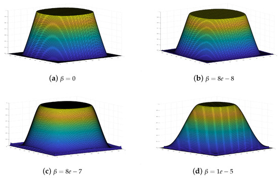
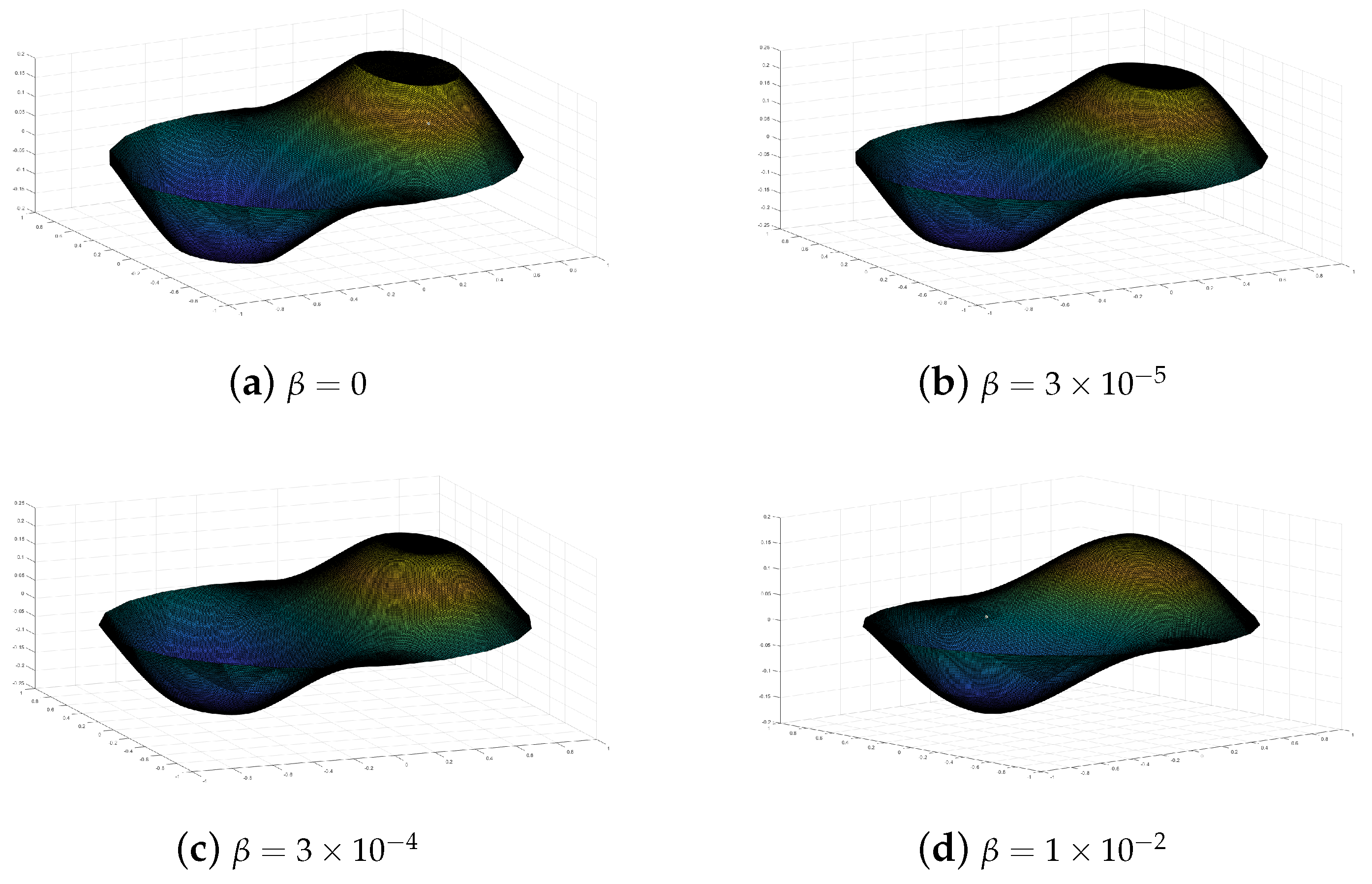
Figure 2. The numerical optimal control, $u_h$, with different values of parameter $\beta$ for Example 2. (a) $u_h$ with $\beta =8\times {10}^{-8}$. (b) $u_h$ with $\beta =0$. (c) $u_h$ with $\beta =8\times {10}^{-7}$. (d) $u_h$ with $\beta =1\times {10}^{-5}$.

We can see from Figure 2 that when $\beta =0$, the numerical optimal control, $u_h$, is not smooth in the cross-section at points a and b. When $\beta >0$, the upper boundary and lower boundary become smooth. Specifically, as the parameter $\beta$ of the gradient penalty term increases, the numerical optimal control, $u_h$, becomes smoother and smoother at the upper and lower boundaries. We can see that introducing a control gradient penalty term into the objective function of PDE-constrained optimization problems can result in a smoother control curve.

As an example, we present the numerical results for $\beta =8\times {10}^{-8}$ for both the three-block ihADMM algorithm and the classical ADMM algorithm in Table 2.

Table 2. The convergence behavior of the three-block ihADMM algorithm and the classical ADMM algorithm.

Case	h	#dofs	Index	Three-Block ihADMM	Classical ADMM
1	${\displaystyle \frac{\sqrt{2}}{2^3}}$	49	#iter	67	71
			Residual $\eta$	$9.64\times {10}^{-7}$	$9.35\times {10}^{-7}$
			CPU time (s)	0.155	0.108
2	${\displaystyle \frac{\sqrt{2}}{2^4}}$	225	#iter	64	71
			Residual $\eta$	$9.20\times {10}^{-7}$	$9.11\times {10}^{-7}$
			CPU time (s)	0.259	0.166
3	${\displaystyle \frac{\sqrt{2}}{2^5}}$	961	#iter	59	68
			Residual $\eta$	$9.31\times {10}^{-7}$	$9.46\times {10}^{-7}$
			CPU time (s)	1.381	0.935
4	${\displaystyle \frac{\sqrt{2}}{2^6}}$	3969	#iter	52	65
			Residual $\eta$	$9.46\times {10}^{-7}$	$9.50\times {10}^{-7}$
			CPU time (s)	5.482	5.424
5	${\displaystyle \frac{\sqrt{2}}{2^7}}$	16,129	#iter	56	89
			Residual $\eta$	$9.87\times {10}^{-7}$	$9.55\times {10}^{-7}$
			CPU time (s)	27.015	78.947
6	${\displaystyle \frac{\sqrt{2}}{2^8}}$	65,025	#iter	206	320
			Residual $\eta$	$8.83\times {10}^{-7}$	$9.99\times {10}^{-7}$
			CPU time (s)	436.688	3285.739
7	${\displaystyle \frac{\sqrt{2}}{2^9}}$	261,121	#iter	354	601
			Residual $\eta$	$8.08\times {10}^{-7}$	$5.39\times {10}^{-5}$
			CPU time (s)	9893.480	87,119.179

The results presented in Table 2 indicate that the proposed three-block ihADMM algorithm demonstrates superior numerical efficiency regarding both the number of iterations and computational time when compared to the classical ADMM algorithm. Furthermore, the fifth and sixth columns of Table 2 show that as the mesh size decreases, the three-block ihADMM algorithm exhibits a more significant advantage in terms of the number of iterations and the computational time compared to the classical ADMM algorithm.

5. Conclusions

In this paper, a new elliptic PDE-constrained optimization model with a control gradient penalty term and pointwise box constraints on the control is proposed to address the application requirements. The main purpose of adding the control gradient penalty term is to smooth the control variable, particularly at the boundary. Nevertheless, adding this penalty term makes the system more complex to solve. To tackle this problem, we introduce two artificial variables and propose a convergent three-block ihADMM algorithm. Unlike the classical ADMM algorithm, the proposed algorithm introduces the inexactness strategy. Moreover, different weighted inner products are adopted to define the augmented Lagrangian function in three subproblems. Theoretically, we present the global convergence analysis and provide theoretical results on the iteration complexity for the proposed algorithm. The numerical experiments demonstrate that the three-block ihADMM algorithm significantly outperforms the classical ADMM algorithm in terms of both the number of iterations and computational time across various final mesh sizes. Moreover, as the final mesh size decreases, the efficiency of the three-block ihADMM algorithm becomes even more obvious.

References

- Huang, F.; Chen, Y.; Chen, Y.; Sun, H. Stochastic collocation for optimal control problems with stochastic PDE constraints by meshless techniques. J. Math. Anal. Appl. 2024, 530, 127634. [Google Scholar] [CrossRef]
- Hinze, M.; Pinnau, R.; Ulbrich, M.; Ulbrich, S. Optimization with PDE Constraints; Springer: Berlin, Germany, 2009; pp. 171–172. [Google Scholar]
- Zheng, Q. A reordering-based preconditioner for elliptic PDE-constrained optimization problems with small Tikhonov parameters. Comp. Appl. Math. 2023, 42, 169. [Google Scholar] [CrossRef]
- Sirignano, J.; MacArt, J.; Spiliopoulos, K. PDE-constrained models with neural network terms: Optimization and global convergence. J. Comput. Phys. 2023, 481, 112016. [Google Scholar] [CrossRef]
- Rudin, L.I.; Osher, S.; Fatemi, E. Nonlinear total variation based noise removal algorithms. Phys. D 1992, 60, 259–268. [Google Scholar] [CrossRef]
- Gao, L.; Ding, J. An improved DMOC method with gradient penalty term. Adv. Mater. Res. 2014, 945, 2784–2787. [Google Scholar] [CrossRef]
- Clever, D.; Lang, J. Optimal control of radiative heat transfer in glass cooling with restrictions on the temperature gradient. Optim. Control Appl. Methods 2012, 33, 157–175. [Google Scholar] [CrossRef]
- Hinze, M.; Vierling, M. The semi-smooth Newton method for variationally discretized control constrained elliptic optimal control problems implementation, convergence and globalization. Optim. Methods Softw. 2012, 27, 933–950. [Google Scholar] [CrossRef]
- Liu, Y.; Wen, Z.; Yin, W. A multiscale semi-smooth Newton method for optimal transport. J. Sci. Comput. 2022, 91, 39. [Google Scholar] [CrossRef]
- Liang, J.; Luo, T.; Schonlieb, C.B. Improving “fast iterative shrinkage-thresholding algorithm”: Faster, smarter, and greedier. SIAM J. Sci. Comput. 2022, 44, A1069–A1091. [Google Scholar] [CrossRef]
- Song, X.; Yu, B.; Wang, Y.; Zhang, X. An FE-inexact heterogeneous ADMM for elliptic optimal control problems with L1-control cost. J. Syst. Sci. Complex. 2018, 31, 1659–1697. [Google Scholar] [CrossRef]
- Chen, X.; Song, X.; Chen, Z.; Yu, B. A multi-level ADMM algorithm for elliptic PDE-constrained optimization problems. Comput. Appl. Math. 2020, 39, 1–31. [Google Scholar] [CrossRef]
- Chen, X.; Song, X.; Chen, Z.; Xu, L. A multilevel heterogeneous ADMM algorithm for elliptic optimal control problems with L1-control cost. Mathematics 2023, 11, 570. [Google Scholar] [CrossRef]
- Chen, Z.; Song, X.; Chen, X.; Yu, B. A warm-start FE-dABCD algorithm for elliptic optimal control problems with constraints on the control and the gradient of the state. Comput. Math. Appl. 2024, 161, 1–12. [Google Scholar] [CrossRef]
- Eckstein, J.; Bertsekas, D. On the Douglas–Rachford splitting method and the proximal point algorithm for maximal monotone operators. Math. Program. 1992, 55, 293–318. [Google Scholar] [CrossRef]
- Eckstein, J. Some saddle-function splitting methods for convex programming. Optim. Methods Softw. 1994, 4, 75–83. [Google Scholar] [CrossRef]
- Bingsheng, H.; Liao, L.; Han, D.; Yang, H. A new inexact alternating directions method for monotone variational inequalities. Math. Program. 2002, 92, 103–118. [Google Scholar]
- Ng, M.K.; Wang, F.; Yuan, X. Inexact alternating direction methods for image recovery. SIAM J. Sci. Comput. 2011, 33, 1643–1668. [Google Scholar] [CrossRef]
- Chen, L.; Sun, D.; Toh, K.C. An efficient inexact symmetric Gauss-Seidel based majorized ADMM for high-dimensional convex composite conic programming. Math. Program. 2017, 161, 237–270. [Google Scholar] [CrossRef]
- Song, X.; Yu, B. A two-phase strategy for control constrained elliptic optimal control problems. Numer. Linear Algebra Appl. 2018, 25, 21–38. [Google Scholar] [CrossRef]
- Chen, C.; He, B.; Ye, Y.; Yuan, X. The direct extension of ADMM for multi-block convex minimization problems is not necessarily convergent. Math. Program. 2016, 155, 57–79. [Google Scholar] [CrossRef]
- Lasdon, L.; Mitter, S.; Waren, A. The conjugate gradient method for optimal control problems. IEEE Trans. Autom. Control. 1967, 12, 132–138. [Google Scholar] [CrossRef]
- Saad, Y.; Schultz, M.H. GMRES: A generalized minimum residual algorithm for solving nonsymmetric linear systems. SIAM J. Sci. Stat. Comput. 1986, 7, 856–869. [Google Scholar] [CrossRef]
- Mora, D.; Rodríguez, R. A piecewise linear finite element method for the buckling and the vibration problems of thin plates. Math. Comput. 2009, 78, 1891–1917. [Google Scholar] [CrossRef]
- Casas, E. Using piecewise linear functions in the numerical approximation of semilinear elliptic control problems. Adv. Comput. Math. 2007, 26, 137–153. [Google Scholar] [CrossRef]
- Wachsmuth, G.; Wachsmuth, D. Convergence and regularization results for optimal control problems with sparsity functional. ESAIM Control Optim. Calc. Var. 2011, 17, 858–886. [Google Scholar] [CrossRef]
- Cao, S.; Wang, Z. PMHSS iteration method and preconditioners for Stokes control PDE-constrained optimization problems. Numer. Algorithms 2021, 87, 365–380. [Google Scholar] [CrossRef]
- Chen, L. iFEM: An Integrated Finite Element Methods Package in MATLAB; Technical report; University of California at Irvine: Irvine, CA, USA, 2008. [Google Scholar]
Disclaimer/Publisher’s Note: The statements, opinions and data contained in all publications are solely those of the individual author(s) and contributor(s) and not of MDPI and/or the editor(s). MDPI and/or the editor(s) disclaim responsibility for any injury to people or property resulting from any ideas, methods, instructions or products referred to in the content. |
© 2024 by the authors. Licensee MDPI, Basel, Switzerland. This article is an open access article distributed under the terms and conditions of the Creative Commons Attribution (CC BY) license (https://creativecommons.org/licenses/by/4.0/).