Beta Autoregressive Moving Average Model with the Aranda-Ordaz Link Function

Abstract

In this work, we introduce an extension of the so-called beta autoregressive moving average ($\beta$ARMA) models. $\beta$ARMA models consider a linear dynamic structure for the conditional mean of a beta distributed variable. The conditional mean is connected to the linear predictor via a suitable link function. We propose modeling the relationship between the conditional mean and the linear predictor by means of the asymmetric Aranda-Ordaz parametric link function. The link function contains a parameter estimated along with the other parameters via partial maximum likelihood. We derive the partial score vector and Fisher’s information matrix and consider hypothesis testing, diagnostic analysis, and forecasting for the proposed model. The finite sample performance of the partial maximum likelihood estimation is studied through a Monte Carlo simulation study. An application to the proportion of stocked hydroelectric energy in the south of Brazil is presented.

1. Introduction

Gaussianity is by far the most commonly used hypothesis in statistics. It is easy to find in the literature applications of Gaussian time series in contexts where it is neither natural nor adequate to suppose normality of the underlying data distribution. Simple examples are strictly positive data such as prices, counting phenomena or double bounded data, such as rates and proportions whose support is $(0,1)$. In these situations, normality is obviously not an adequate hypothesis to assume. The consequences of using a Gaussian time series model were it is not reasonable may be grave, especially when the focus lies on forecasting. In these cases, it is a common problem to obtain predicted values that lie outside the natural bounds of the data.

To overcome these issues, non-Gaussian time series models have been extensively explored in the literature. For instance, autoregressive models for integer valued time series were introduced in [1]. A broad class of dynamic models for non-Gaussian time series based on generalized linear models (GLM) [2] was considered in [3], which called them generalized autoregressive moving average (GARMA) models. Traditional GLM methods can serve as an inspiration for time series models, but there are important distinctions and technicalities to keep in mind [4]. Other studies in this direction can be found in [5,6,7,8].

Modeling rates and proportions observed over time is a common problem in many areas of application. By nature, such time series are limited to the interval $(0,1)$ and, hence, Gaussianity is an assumption that should be avoided [9]. In this direction, the class of beta autoregressive moving average ($\beta$ARMA) models, proposed by [10], introduces a GLM-like dynamic model for time series restricted to $(0,1)$. The $\beta$ARMA model assume that, conditionally to its past, the variable of interest follows a beta distribution while the conditional mean is modeled through a dynamical time dependent linear structure accommodating an ARMA-like term and a linear combination of exogenous covariates. The conditional mean is connected to the linear predictor through a suitable fixed link function.

The beta distribution is well known for its flexibility, being able to model asymmetric behaviors such as bathtub and J-shaped and inverted J-shaped densities, among other. For this reason, the literature has seen a growing interest in beta-based models in the last decade and several improvements and generalizations of the $\beta$ARMA model have been proposed. For instance, some generalizations propose the use of different specifications for the systematic component. Ref. [11] proposed the class of $\beta$SARMA models which introduces a seasonal ARMA structure in the systematic components. Ref. [12] proposed the class of $\beta$ARFIMA models by considering a long range dependent specification for the systematic component. Some goodness-of-fit tests for $\beta$ARMA are proposed in [13], while prediction intervals and model selection criteria are recently explored in [14,15], respectively. In [16], the inflated $\beta$ARMA model was introduced for modeling time series data that assume values in the intervals $(0,1]$, $[0,1)$ or $[0,1]$.

A common feature in the aforementioned models, i.e., the connection between the conditional mean with the linear predictor is made by a suitable link function, ensures that the modeled conditional mean values do not fall outside its natural bounds. Typical choices for responses taking values in $(0,1)$ are the logit and cloglog fixed links. However, misspecification of the link function may cause distortions in parameter estimation [2]. A simple solution to this problem is to apply a parametric link function. This adds flexibility to the model and improves the finite sample performance of maximum likelihood estimation in the context of GLM [17], compared to the canonical ones. In the literature, we can find some models that apply parametric link functions in the context of regression models. For instance, for binary response problems, [18] proposed the use a modified Box-Cox transformation as link function, while [19] introduced a modified two parameter link that allows free manipulation of both tails of the link. More flexible approaches, which treat the entire link function to be estimated from the data, were considered in [20,21,22]. In the context of beta regression with variable dispersion, [23] proposed the use of parametric link function for the specification of both, mean and dispersion. Recently, ref. [24] proposed the use of the Aranda-Ordaz parametric link function [25] in the context of Kumaraswamy regression. Other applications of parametric link functions in regression models can be found in [26,27,28,29].

Despite the relative growth of the literature on parametric link function in regression models, to the best of our knowledge, there are no time series models considering parametric link functions. In this direction, this works generalizes the $\beta$ARMA model by introducing a parametric link function in the conditional mean specification. Given that a time series following a $\beta$ARMA lies on $(0,1)$, a suitable and widely known link (as discussed in [23]) is the Aranda-Ordaz asymmetric link function, introduced in [25]. The Aranda-Ordaz link function depends on a parameter $\lambda$ which must be known, or, ideally, estimated from the data. To do that, we propose a partial maximum likelihood approach to estimate $\lambda$ along with all other parameters in the model.

Different from time series analysis, in regression analysis, the interpretability of the fitted model is of great interest. Some commonly applied link functions, such as the logit and logarithm, allow for a simple interpretation of model parameters, which is no longer the case when we consider a parametric specification for the link function. However, in time series models, prediction is usually considered more important than model interpretability, which favors the use of a parametric link function, since it usually allows for a better model fitting and, often, a superior forecasting performance. In this sense, the proposed $\beta$ARMA with Aranda-Ordaz link function provides two advantages over the standard $\beta$ARMA model: (i) better model fitting due to more flexibility when considering the relationship between the mean and the linear predictor and (ii) robustness against inferential distortions usually attributed to link misspecification.

The paper is organized as follows. In the next section, we introduce the $\beta$ARMA model with the Aranda-Ordaz link function. In Section 3, we propose a partial maximum likelihood approach to estimate the model parameters and discuss some of its properties. In Section 4, we present some diagnostic and goodness-of-fit tools and discuss forecasting in the context of the proposed model. A Monte Carlo simulation study is presented in Section 5, while a real data application is presented in Section 6. Our conclusions are presented in Section 7 and some technical details are discussed in the Appendix A and Appendix B.

2. Proposed Model

Let ${\left\{y_t\right\}}_{t\in \mathbb{Z}}$ denote a time series of interest and let ${\left\{{\mathit{x}}_t\right\}}_{t\ge 1}$ denote a set of k-dimensional exogenous covariates, possibly time dependent and random. Let ${\mathcal{F}}_t$ denote the $\sigma$-field representing the history of the model known to the researcher up to time t, that is, the sigma-field generated by $(y_t,{\mathit{x}}_t^{\prime },y_{t-1},{\mathit{x}}_{t-1}^{\prime },y_{t-2},{\mathit{x}}_{t-2}^{\prime },\cdots )$. We assume that the conditional distribution of $y_t$ given ${\mathcal{F}}_{t-1}$ is $\mathrm{Beta}({\mu }_t,\varphi )$ parameterized as in [9], with density:

$$f\left(y_t\right|{\mathcal{F}}_{t-1})={\displaystyle \frac{\Gamma \left(\varphi \right)}{\Gamma \left({\mu }_t\varphi \right)\Gamma \left((1-{\mu }_t)\varphi \right)}}{y}_t^{{\mu }_t\varphi -1}{(1-y_t)}^{(1-{\mu }_t)\varphi -1},0<y_t<1,$$

(1)

where $\Gamma (·)$ is the Gamma function, $0<{\mu }_t<1$ and $\varphi >0$. It is easy to show that:

$$\mathbb{E}\left(y_t\right|{\mathcal{F}}_{t-1})={\mu }_t\mathrm{and}\mathrm{Var}\left(y_t\right|{\mathcal{F}}_{t-1})={\displaystyle \frac{{\mu }_t(1-{\mu }_t)}{1+\varphi }}.$$

Observe that the parameter $\varphi$ acts as a precision parameter, since the higher the $\varphi$, the smaller the variance of $y_t$, for a fixed ${\mu }_t$. Note that the variance of $y_t$ changes for each t, so the model is naturally heteroscedastic. Although, in principle, it could be possible to consider a variable dispersion parameter, as in [23]; however, the majority of works in the literature assume a constant precision/dispersion parameter ([3,9,10,11,15,30], to name just a few) so, for simplicity, we shall do the same.

Let $g(·,\lambda ):(0,1)\to \mathbb{R}$ be a twice continuously differentiable one to one link function, possibly depending on a parameter $\lambda$. Consider the following specification for the model’s systematic component:

$${\eta }_t≔g({\mu }_t,\lambda )=\alpha +{\mathit{x}}_t^{\top }\mathit{\beta }+\sum _{i=1}^p{\phi }_i\left[g(y_{t-i},\lambda )-{\mathit{x}}_{t-i}^{\top }\mathit{\beta }\right]+\sum _{j=1}^q{\theta }_j{r}_{t-j},$$

(2)

where $\alpha \in \mathbb{R}$ is an intercept, $\mathit{\beta }={({\beta }_1,\dots ,{\beta }_k)}^{\top }\in {\mathbb{R}}^k$ is a k-dimensional vector of parameter associated with the covariates, and $\mathit{\phi }≔{({\phi }_1,\dots ,{\phi }_p)}^{\top }$ and $\mathit{\theta }≔{({\theta }_1,\dots ,{\theta }_q)}^{\top }$ are p and q-dimensional vectors of parameters associated with the autoregressive and moving average components, respectively. The error term is defined as $r_t=g(y_t,\lambda )-g({\mu }_t,\lambda )$. Observe that if we substitute $g(y,\lambda )$ for a fixed (non-parametric) link function $g\left(y\right)$, such as logit or probit links, then we obtain the $\beta$ARMA model of [10].

In (2), when g indeed depends on $\lambda$ we have a parametric link function. The choice of the parametric link is an important one and due to its flexibility, we shall apply the asymmetric Aranda-Ordaz family of link functions in (2), which has the form:

$${\eta }_t=g({\mu }_t,\lambda )=\log \left({\displaystyle \frac{{(1-{\mu }_t)}^{-\lambda }-1}{\lambda }}\right),$$

(3)

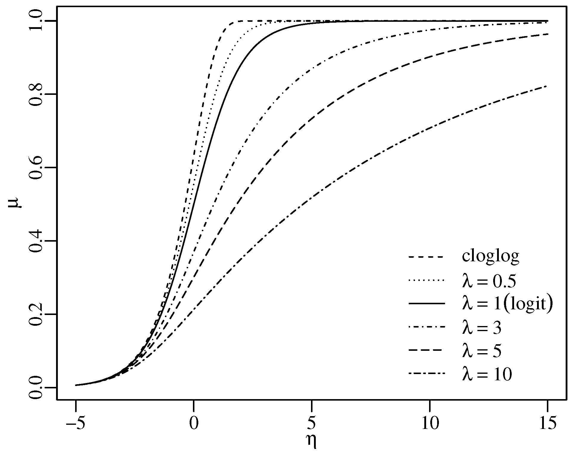
for $\lambda >0$. Observe that ${\mu }_t=g^{-1}({\eta }_t,\lambda )=1-{\left[1+\lambda \exp \left({\eta }_t\right)\right]}^{-{\displaystyle \frac{1}{\lambda }}}$ and that g is infinitely differentiable away from zero on $\lambda$ and $\mu$. Figure 1 shows the Aranda-Ordaz link function for several values of $\lambda$, highlighting its asymmetric behavior, which allows an asymmetric relationship between ${\mu }_t$ and ${\eta }_t$. We note that it is an increasing and monotonic function, where positive (or negative) changes in the linear predictor imply a positive (or negative) effect on the response mean. The traditional logit is a particular case obtained when $\lambda =1$ and the cloglog is obtained as a limiting case for $\lambda \to 0$.

Figure 1. The Aranda-Ordaz link function for different values of $\lambda$.

The proposed $\beta$ARMA model with Aranda-Ordaz link function, hereafter referred to as $\beta {\mathrm{ARMA}}_{\lambda }$, is defined by (1), (2), and (3). The Aranda-Ordaz parameter influences the conditional mean ${\mu }_t$, which affects the response $Y_t$ through $Y_t|{\mathcal{F}}_{t-1}\sim \mathrm{Beta}({\mu }_t,\varphi )$. Figure 1 illustrates how the parameter $\lambda$ affects ${\mu }_t$ as a function of ${\eta }_t$. For $0<\lambda <1$, the effect on ${\mu }_t$ is mild compared to clolog and logit, primarily impacting ${\eta }_t$ values between 0 and 4 by slightly accelerating or decelerating the increase of ${\mu }_t$ relative to ${\eta }_t$. For $\lambda >1$, the impact of $\lambda$ is more pronounced, with larger $\lambda$ values dampening the speed at which changes in ${\eta }_t$ affect ${\mu }_t$. Thus, for $\lambda >1$, ${\mu }_t$ becomes less sensitive to variations in ${\eta }_t$, smoothing $Y_t$’s conditional mean compared to the logit and cloglog functions.

3. Partial Likelihood Inference

Let ${\left\{({\mathit{x}}_t,y_t)\right\}}_{t=1}^n$ be a sample from the proposed $\beta {\mathrm{ARMA}}_{\lambda }$ model and let $\mathit{\omega }≔{(\varphi ,\lambda ,\alpha ,{\mathit{\beta }}^{\top },{\mathit{\phi }}^{\top },{\mathit{\theta }}^{\top })}^{\top }$ be the $(p+q+k+3)$-dimensional vector of unknown parameters in the model, and $\mathsf{\Omega }={(0,\infty )}^2\times {\mathbb{R}}^{1+k+p+q}$ is the parametric space, such that $\mathit{\omega }\in \mathsf{\Omega }$. In this section, we derive a partial maximum likelihood estimation (PMLE) approach to estimate $\mathit{\omega }$. Given ${\mathcal{F}}_{t-1}$, the partial log-likelihood function is given by:

$$\begin{array}{c}\hfill \ell \left(\mathit{\omega }\right)≔\sum _{t=m+1}^n\log f\left(y_t\right|{\mathcal{F}}_{t-1})=\sum _{t=m+1}^n{\ell }_t({\mu }_t,\varphi ),\end{array}$$

(4)

where $m=\max \{p,q\}$ and

$$\begin{array}{cc}\hfill {\ell }_t({\mu }_t,\varphi )& ≔\log \left(\Gamma \left(\varphi \right)\right)-\log \left(\Gamma \left({\mu }_t\varphi \right)\right)-\log \left(\Gamma \left[(1-{\mu }_t)\varphi \right]\right)\hfill \\ & +({\mu }_t\varphi -1)\log \left(y_t\right)+\left[(1-{\mu }_t)\varphi -1\right]\log (1-y_t).\hfill \end{array}$$

The estimator $\widehat{\mathit{\omega }}$ is defined as:

$$\begin{array}{c}\hfill \widehat{\mathit{\omega }}≔\arg \underset{\mathit{\omega }\in \mathsf{\Omega }}{\sup }\left\{\ell \left(\omega \right)\right\}.\end{array}$$

(5)

The solution of (5) is obtained by solving $U\left(\mathit{\omega }\right)=\mathbf{0}$, where $U\left(\mathit{\omega }\right)$ is the partial score vector and $\mathbf{0}≔{(0,\dots ,0)}^{\top }\in {\mathbb{R}}^{p+q+k+3}$. Closed-form expressions of the partial score vector are presented in Appendix A.

The non-linear system $U\left(\mathit{\omega }\right)=\mathbf{0}$ has no closed-form solution. To obtain approximate solutions, it is necessary to numerically maximize the partial log-likelihood function given in (4). In this work, we consider the so-called BFGS method [31] with analytical first derivatives to do so. The procedure requires initialization. We initialize $\lambda =1$ (logit particular case) and $\mathit{\theta }=\mathbf{0}$ in all cases. Parameters $\alpha$, $\mathit{\beta }$, and $\mathit{\phi }$ are initialized as the ordinary least squares estimates of the regression problem:

$$g(y_t,1)=\alpha +{\mathit{x}}_t^{\top }\mathit{\beta }+\sum _{i=1}^p{\phi }_{i}g(y_{t-i},1)+{\epsilon }_t,$$

where ${\epsilon }_t$ denotes an error term. Let ${({\alpha }^0,{\mathit{\beta }}^0,{\mathit{\phi }}^0)}^{\top }$ denote the initial value of ${(\alpha ,\mathit{\beta },\mathit{\phi })}^{\top }$, the starting value of $\varphi$ is given by:

$${\varphi }^0≔{\displaystyle \frac{1}{n}}\sum _{t=1}^n{\displaystyle \frac{{\mu }_t^0(1-{\mu }_t^0)}{{\mathfrak{s}}^0}}-1,$$

where ${\mu }_t^0≔g^{-1}\left({\alpha }^0+{\mathit{x}}_t^{\top }{\mathit{\beta }}^0+{\sum }_{i=1}^p{\phi }_i^0\left[g(y_{t-i},1)-{\mathit{x}}_{t-i}^{\top }{\mathit{\beta }}^0\right],1\right)$ and ${\displaystyle {\mathfrak{s}}^0≔\frac{1}{n-1}\sum _{t=1}^n{\left(y_t-{\mu }_t^0\right)}^2}$.

In addition to point inference, it is also interesting to build confidence intervals and carry out hypothesis tests. In this sense, we need the asymptotic distribution of the partial maximum likelihood estimator. The seminal work of  [32] established the asymptotic theory of the maximum likelihood in the context of traditional GLM under mild conditions. These results were generalized for the case of GLM with parametric link functions in [33]. For GARMA-like models, a rigorous asymptotic theory was established in [34,35]. Ref. [12] presented the asymptotic theory for the PMLE in the context of $\beta$ARFIMA models. Recently, Ref. [24] established the asymptotic theory of the MLE for GLM-like models with the Aranda-Ordaz parametric link based on the Kumaraswamy distribution, which is not a member of the exponential family.

In the context of $\beta {\mathrm{ARMA}}_{\lambda }$ model, specification (1) and the fact that the information matrix is not block diagonal imply that the parameter estimation must be jointly performed via the log-likelihood function. To derive the asymptotic theory for the PMLE in the context of the present work, a similar argument as in [33,34] can be applied, with a few modifications. Under suitable conditions, closely related to the ones presented in [34], it can be shown that the partial maximum likelihood estimator $\widehat{\mathit{\omega }}$ is consistent and:

$$\sqrt{n}(\widehat{\mathit{\omega }}-\mathit{\omega })\stackrel{d}{⟶}\mathcal{N}(\mathbf{0},K^{-1}\left(\mathit{\omega }\right)),$$

as n tends to infinity, where $\mathcal{N}(\mathbf{0},\mathsf{\Sigma })$ denotes the $(p+q+k+3)$-variate normal distribution with mean vector $\mathbf{0}$ and variance-covariance matrix $\mathsf{\Sigma }$. The matrix $K\left(\mathit{\omega }\right)$ is a positive definite and invertible matrix, the analogous to the information matrix per observation in the context of i.i.d. samples. Under suitable conditions, $K_n\left(\mathit{\omega }\right)/n⟶K\left(\mathit{\omega }\right)$ in probability, where $K_n\left(\mathit{\omega }\right)$ is the cumulative conditional information matrix presented in the Appendix B.

Let ${\omega }_r$ denote the r-th component of $\mathit{\omega }$, and with the previous results, it is possible to obtain approximate confidence interval to ${\omega }_r$ and standard Z statistics to test hypothesis like ${\mathcal{H}}_0:{\omega }_r={\omega }_r^0$ vs. ${\mathcal{H}}_1:{\omega }_r\ne {\omega }_r^0$ [36]. Versions of other commonly applied test statistics, such as the Wald [37], likelihood ratio [38], Rao’s score [39], and the gradient [40] statistic, can be similarly defined. Their asymptotic distributions will be ${\chi }^2$ with the corresponding degrees of freedom imposed by the restrictions under ${\mathcal{H}}_0$. More general forms of these hypothesis tests can be performed similarly to traditional regression models.

4. Diagnostics and Forecasting

In this section, we consider some diagnostic tools useful in determining whether a fitted model succeeded in capturing the data dynamics. Also, we detail a method to produce forecasts based on a fitted model. Besides the joint significance of the parameters obtained using the tests presented in the previous section, we can also discuss residual analysis. A priori, there is no imposed distributional structure for the error term $r_t$ in (2), but it is quite common to look at some goodness-of-fit statistics.

The so-called deviance statistics is commonly applied as a goodness-of-fit measure of a given model [4]. It can be shown that, if the model is correctly specified, then the deviance statistics is asymptotically ${\chi }_{n-(p+q+k+3)}^2$ distributed [3,4]. Model selection can be performed by using adapted versions of the AIC [41] and BIC [42]. A lower AIC and BIC values are associated with more suitable models. Residual analysis is a fundamental diagnostic tool in statistical modeling. There are several ways to define the residuals for the proposed model, such as standardized, quantile [43], and deviance residuals. As considered in [13], for the $\beta$ARMA, and in [9], for the beta regression model, we suggest using the standardized ordinary residual.

Another useful tool in diagnostic analysis are Portmanteau tests. If the model is correctly specified, it is expected that the residuals behave like a white noise [4]. Portmanteau tests for $\beta$ARMA models were rigorously studied by [13]. In this context, similar arguments to those in [13] can be applied to show that the Ljung–Box statistics to test the null hypothesis that the first s residual autocorrelations are zero will be asymptotically ${\chi }_{s-p-q}^2$ distributed, under mild assumptions.

Since the proposed model is an extension of the $\beta$ARMA, $h_0$-step ahead forecasts can be obtained similarly. Let ${\left\{({\mathit{x}}_t,y_t)\right\}}_{t=1}^n$ be a sample from the proposed $\beta {\mathrm{ARMA}}_{\lambda }$ model. Let $\widehat{\mathit{\omega }}$ be the PMLE based on the sample and ${\widehat{\mu }}_t$ be ${\mu }_t$ evaluated at $\widehat{\mathit{\omega }}$ and $\widehat{r_t}≔\left[g(y_t,\widehat{\lambda })-g(\widehat{{\mu }_t},\widehat{\lambda })\right]I(1\le t\le n)$. For $h=1,2,\dots ,h_0$, h-step ahead forecasts are given by:

$$\begin{array}{c}\hfill {\widehat{\mu }}_{n+h}≔g^{-1}\left(\widehat{\alpha }+{\mathit{x}}_{n+h}^{\top }\widehat{\mathit{\beta }}+\sum _{i=1}^p\widehat{{\phi }_i}\left(\left[g(y_{n+h-i},\widehat{\lambda })\right]-{\mathit{x}}_{n+h-i}^{\top }\widehat{\mathit{\beta }}\right)+\sum _{j=1}^q\widehat{{\theta }_j}{\widehat{r}}_{n+h-j},\widehat{\lambda }\right),\end{array}$$

where $\left[g(y_t,\lambda )\right]≔\left\{\begin{array}{cc}\hfill g(\widehat{{\mu }_t},\widehat{\lambda }),& \mathrm{if}t>n,\hfill \\ \hfill g(y_t,\widehat{\lambda }),& \mathrm{if}t\le n.\hfill \end{array}\right.$

5. Numerical Experiments

In this section, we present a Monte Carlo simulation study to assess the finite sample properties of the PMLE for the proposed model parameters. We consider 10,000 simulated replications of a process ${\left\{y_t\right\}}_{t=1}^n$, for $n\in \{100,300,500,1000\}$ following the $\beta {\mathrm{ARMA}}_{\lambda }$$(p,q)$. The following two scenarios were considered in the simulation:

• $\beta {\mathrm{ARMA}}_{\lambda }$$(2,2)$ with two covariates, where the parameters are set as $\alpha =0.5$, $\mathit{\beta }={(0.3,-1)}^{\top }$, $\mathit{\phi }={(-0.5,0.3)}^{\top }$, $\mathit{\theta }={(0.4,-0.1)}^{\top }$, $\varphi \in \{20,120\}$, and $\lambda =1.5$;
• $\beta {\mathrm{ARMA}}_{\lambda }$$(2,1)$ with one covariate, where the parameters are $\alpha =-0.5$, ${\beta }_1=-1$, $\mathit{\phi }={(-0.4,0.2)}^{\top }$, ${\theta }_1=0.3$, $\varphi \in \{20,120\}$, and $\lambda =0.5$.

In order to induce a deterministic seasonality into the model, we consider ${\mathit{x}}_t={\left(\sin (2\pi t/12),\cos (2\pi t/12)\right)}^{\top }$ in Scenario 1 and $x_t=\cos \left(2\pi t/12\right)$ in Scenario 2. All simulations were performed using R version 3.5.2 [44]. Table 1 and Table 2 present the simulation results for Scenario 1, while Table 3 and Table 4 for Scenario 2 by varying the precision parameter $\varphi \in \{20,120\}$. Presented are the mean estimate, relative bias (RB), standard error (SE), and mean square error (MSE).

Table 1. Simulation results for the proposed PMLE under Scenario 1 with $\varphi =120$.

	$\alpha$	${\beta }_1$	${\beta }_2$	${\phi }_1$	${\phi }_2$	${\theta }_1$	${\theta }_2$	$\lambda$	$\varphi$
	0.5	0.3	−1	−0.5	0.3	0.4	−0.1	1.5	120
$n=100$
Mean	0.693	0.253	−1.050	−0.488	0.281	0.308	−0.036	1.820	132.753
RB (%)	38.631	−15.801	4.965	−2.328	−6.299	−22.944	−64.227	21.361	10.627
SE	2.660	0.319	0.424	0.603	0.689	0.616	0.529	3.887	20.858
MSE	7.115	0.104	0.182	0.364	0.474	0.387	0.284	15.212	597.688
$n=300$
Mean	0.549	0.282	−1.022	−0.549	0.290	0.416	−0.064	1.545	124.046
RB (%)	9.772	−6.107	2.197	9.707	−3.466	3.876	−35.550	3.021	3.371
SE	0.394	0.038	0.164	0.407	0.391	0.427	0.328	0.500	10.420
MSE	0.158	0.002	0.027	0.168	0.153	0.183	0.109	0.253	124.945
$n=500$
Mean	0.532	0.282	−1.016	−0.524	0.324	0.397	−0.093	1.532	122.285
RB (%)	6.429	−5.978	1.648	4.734	7.847	−0.840	−6.583	2.104	1.904
SE	0.321	0.027	0.124	0.327	0.315	0.342	0.265	0.379	7.810
MSE	0.104	0.001	0.016	0.108	0.100	0.117	0.070	0.144	66.225
$n=1000$
Mean	0.539	0.283	−1.016	−0.523	0.330	0.400	−0.095	1.531	121.149
RB (%)	7.747	−5.601	1.619	4.640	9.954	0.099	−4.635	2.044	0.957
SE	0.226	0.019	0.086	0.225	0.217	0.233	0.181	0.260	5.395
MSE	0.053	0.001	0.008	0.051	0.048	0.054	0.033	0.069	30.430

Table 2. Simulation results for the proposed PMLE under Scenario 1 with $\varphi =20$.

	$\alpha$	${\beta }_1$	${\beta }_2$	${\phi }_1$	${\phi }_2$	${\theta }_1$	${\theta }_2$	$\lambda$	$\varphi$
	0.5	0.3	−1	−0.5	0.3	0.4	−0.1	1.5	20
$n=100$
Mean	2.197	0.161	−1.295	−0.657	0.450	0.363	−0.004	3.855	22.678
RB (%)	339.318	−46.389	29.453	31.354	49.996	−9.144	−96.077	156.990	13.389
SE	7.309	0.960	1.079	0.952	1.372	0.634	0.538	10.157	3.650
MSE	56.303	0.942	1.251	0.932	1.904	0.404	0.298	108.704	20.491
$n=300$
Mean	0.910	−0.595	0.302	0.448	−0.044	20.698	1.964	0.253	−1.098
RB (%)	81.931	19.038	0.792	12.098	−56.266	3.491	30.966	−15.671	9.753
SE	3.505	0.447	0.604	0.429	0.325	1.702	4.698	0.450	0.529
MSE	12.454	0.208	0.365	0.186	0.109	3.384	22.290	0.205	0.289
$n=500$
Mean	0.624	0.282	−1.040	−0.566	0.292	0.439	−0.063	1.576	20.400
RB (%)	24.788	−6.031	4.038	13.232	−2.588	9.711	−37.279	5.073	2.002
SE	0.812	0.093	0.282	0.331	0.320	0.337	0.257	0.955	1.297
MSE	0.675	0.009	0.081	0.114	0.102	0.115	0.067	0.918	1.841
$n=1000$
Mean	0.557	0.282	−1.015	−0.546	0.308	0.423	−0.078	1.511	20.191
RB (%)	11.455	−5.869	1.485	9.203	2.685	5.827	−22.212	0.730	0.953
SE	0.397	0.038	0.169	0.226	0.216	0.231	0.176	0.503	0.881
MSE	0.161	0.002	0.029	0.053	0.047	0.054	0.031	0.253	0.813

Table 3. Simulation results for the proposed PMLE under Scenario 2 with $\varphi =120$.

	$\alpha$	${\beta }_1$	${\phi }_1$	${\phi }_2$	${\theta }_1$	$\lambda$	$\varphi$
	−0.5	−1.0	−0.4	0.2	0.3	0.5	120
$n=100$
Mean	−0.433	−1.048	−0.314	0.160	0.207	0.629	130.483
RB (%)	−13.354	4.850	−21.569	−20.199	−30.895	25.739	8.735
SE	0.248	0.119	0.389	0.119	0.413	0.394	19.982
MSE	0.066	0.016	0.159	0.016	0.179	0.171	509.160
$n=300$
Mean	−0.518	−1.015	−0.408	0.149	0.307	0.534	122.941
RB (%)	3.636	1.511	1.946	−25.272	2.486	6.765	2.451
SE	0.159	0.073	0.206	0.067	0.212	0.246	10.199
MSE	0.025	0.006	0.042	0.007	0.045	0.062	112.665
$n=500$
Mean	−0.531	−0.427	0.149	0.329	121.462	0.525	−1.011
RB (%)	6.222	6.823	−25.370	9.795	1.219	5.020	1.068
SE	0.127	0.144	0.050	0.149	7.765	0.197	0.059
MSE	0.017	0.022	0.005	0.023	62.427	0.040	0.004
$n=1000$
Mean	−0.541	−1.008	−0.442	0.147	0.345	0.518	120.628
RB (%)	8.180	0.753	10.413	−26.418	14.834	3.574	0.523
SE	0.088	0.041	0.094	0.035	0.098	0.139	5.375
MSE	0.009	0.002	0.011	0.004	0.012	0.020	29.288

Table 4. Simulation results for the proposed PMLE under Scenario 2 with $\varphi =20$.

	$\alpha$	${\beta }_1$	${\phi }_1$	${\phi }_2$	${\theta }_1$	$\lambda$	$\varphi$
	−0.5	−1.0	−0.4	0.2	0.3	0.5	20
$n=100$
Mean	−0.091	−1.240	−0.345	0.197	0.211	1.332	21.745
RB (%)	−81.898	24.005	−13.710	−1.590	−29.671	166.329	8.727
SE	2.411	1.075	0.444	0.180	0.390	5.924	3.253
MSE	5.979	1.213	0.200	0.032	0.160	35.784	13.629
$n=300$
Mean	−0.406	−1.080	−0.381	0.179	0.282	0.733	20.565
RB (%)	−18.707	7.985	−4.638	−10.545	−5.972	46.634	2.824
SE	0.248	0.150	0.204	0.074	0.209	0.464	1.710
MSE	0.070	0.029	0.042	0.006	0.044	0.270	3.244
$n=500$
Mean	−0.448	−1.051	−0.387	0.175	0.292	0.653	20.289
RB (%)	−10.381	5.118	−3.291	−12.493	−2.803	30.606	1.445
SE	0.196	0.118	0.147	0.055	0.152	0.371	1.264
MSE	0.041	0.017	0.022	0.004	0.023	0.161	1.681
$n=1000$
Mean	−0.483	−1.030	−0.398	0.171	0.306	0.592	20.136
RB (%)	−3.365	3.032	−0.486	−14.723	1.915	18.495	0.678
SE	0.143	0.086	0.099	0.039	0.102	0.272	0.878
MSE	0.021	0.008	0.010	0.002	0.010	0.083	0.789

As expected, in general, as n increases, the mean of the estimated values converges to the true value of the parameter and the RB, SE, and MSE decrease. Note that for $\varphi =20$, the relative bias and standard errors are higher than the ones when $\varphi =120$. This behavior is expected since decreasing precision implies an increase in the variability of $y_t$. For small sample sizes such as $n=100$, there is considerable bias in all scenarios. Just as in the case of the beta regression [45] and $\beta$ARFIMA [12], $\widehat{\varphi }$ is slightly biased, especially in small samples.

Overall, all parameters are reasonably estimated even in small samples. In all scenarios, the MSE uniformly decreases as n increases, which represents numerical evidence of the PMLE’s consistency. Among all parameters, the estimation of $\alpha$ is the one presenting the highest relative bias. The simulation results provide numerical evidence supporting the theory discussed in Section 3.

6. Application

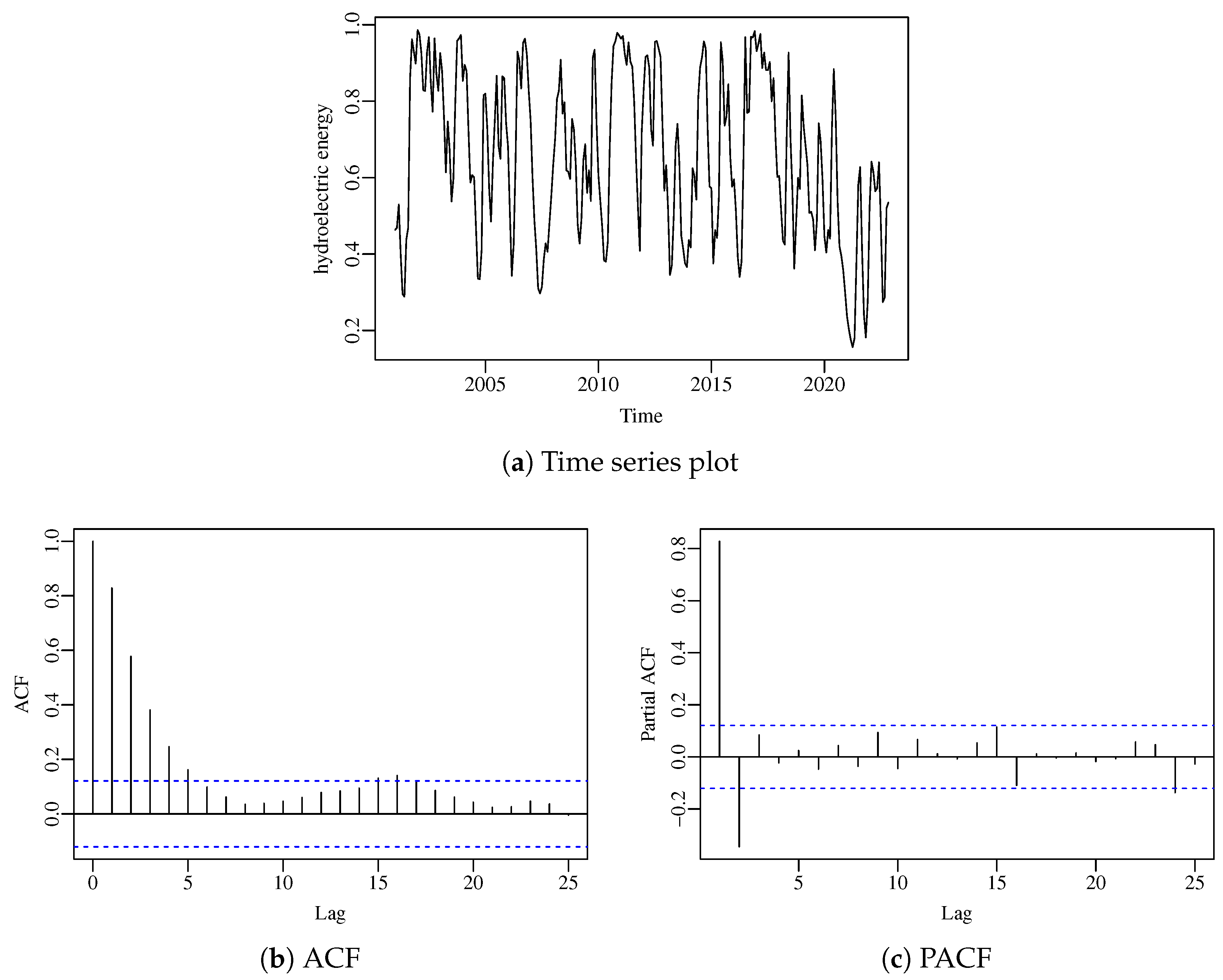
In this section, we showcase the usefulness of the proposed $\beta {\mathrm{ARMA}}_{\lambda }$ model in a real data application. The data comprehend the monthly proportion of stocked hydroelectric energy in the south of Brazil from January 2000 to May 2022, yielding a total of 269 observations. The last six months of data were reserved for out-of-sample forecasting purposes, and hence, for modeling purposes the sample size is $n=263$. This is an updated time series that was also modeled in [13]. The data are freely available at the Operador Nacional do Sistema Elétrico repository (http://www.ons.org.br/paginas/resultados-da-operacao/historico-da-operacao/dados-gerais/, accessed on 29 October 2024). The hydrological study is essential for the adequate distribution of energy and to supply the consumption demand of the population. Forecasts are widely used by institutions to prevent energy shortages. All the results presented in this section can be accessed by a friendly web application available at http://ufsm.shinyapps.io/appBARMA/, accessed on 29 October 2024. In this online application, users can upload any time series data to fit using the proposed model.

Figure 2 presents the time series plot of the data, as well as its sample autocorrelation (ACF) and partial autocorrelation (PACF) functions. From the time series plot, a clear yearly seasonal pattern can be observed. In order to capture this seasonality, we shall employ ${\mathit{x}}_t=\sin (2\pi t/12)$ as covariate in the model.

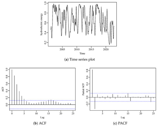
Figure 2. Time series and related plots for the hydroelectric energy.

Additionally, we consider a further step in the optimization procedure that explores different initial values of $\lambda$ (Aranda-Ordaz parameter); this step selects the model that has the smallest AIC value. The algorithm is described by:

• Let ${\mathit{\lambda }}^0={({\lambda }_1^0,\dots ,{\lambda }_L^0)}^{\top }\in {(0,\infty )}^L$ be a vector of initial values associated with the Aranda-Ordaz link function parameter.
• Fit L models, one for each ${\lambda }_l^0$, for $l\in \{1,\dots ,L\}$.
• Calculate the AIC for each fitted model and choose the one with the lowest value.

For this application, we considered ${\mathit{\lambda }}^0={(0.5,1,3,5)}^{\top }$.

Model selection is carried out in a similar fashion to the iterative Box and Jenkins methodology [46]. To select the model, first we compare the AIC of the following competing models: $\beta {\mathrm{AR}}_{\lambda }\left(1\right)$, $\beta {\mathrm{AR}}_{\lambda }\left(2\right)$, $\beta {\mathrm{AR}}_{\lambda }\left(3\right)$, $\beta {\mathrm{MA}}_{\lambda }\left(1\right)$, $\beta {\mathrm{MA}}_{\lambda }\left(2\right)$, $\beta {\mathrm{MA}}_{\lambda }\left(3\right)$, $\beta {\mathrm{ARMA}}_{\lambda }$$(1,1)$, $\beta {\mathrm{ARMA}}_{\lambda }$$(2,1)$, $\beta {\mathrm{ARMA}}_{\lambda }$$(3,1)$, $\beta {\mathrm{ARMA}}_{\lambda }$$(1,2)$, $\beta {\mathrm{ARMA}}_{\lambda }$$(1,3)$, $\beta {\mathrm{ARMA}}_{\lambda }$$(2,2)$, $\beta {\mathrm{ARMA}}_{\lambda }$$(3,2)$, $\beta {\mathrm{ARMA}}_{\lambda }$$(2,3)$, and $\beta {\mathrm{ARMA}}_{\lambda }$$(3,3)$. The model selected by the AIC was a $\beta {\mathrm{ARMA}}_{\lambda }$$(2,1)$ given by:

$${\eta }_t=g({\mu }_t,\lambda )=\alpha +{\beta }_1\sin (2\pi t/12)+{\phi }_2\left[g(y_{t-2},\lambda )-{\beta }_1\sin (2\pi (t-2)/12)\right]+{\theta }_1{r}_{t-1}.$$

The parameter ${\phi }_1$ was not significant. Table 5 presents a summary of the fitted model with estimated parameters, standard errors, Z-statistics, and p-values, as well as AIC, BIC, deviance, and Ljung–Box test for the residuals. We also test the null hypothesis ${\mathcal{H}}_0:\lambda =1$ (logit), rejecting the null hypothesis at the 1% significance level, indicating that the logit function is not adequate for the data.

Table 5. Summary statistics for the fitted $\beta {\mathrm{ARMA}}_{\lambda }$$(2,1)$.

	Estimate	Std. Error	Z Statistic	p-Value
$\alpha$	0.616	0.249	2.478	0.013
${\phi }_2$	0.445	0.109	4.090	<0.001
${\theta }_1$	0.840	0.062	13.634	<0.001
${\beta }_1$	−0.424	0.163	2.600	0.009
$\lambda$	1.920	0.264	7.284 *	<0.001
$\varphi$	12.482	1.073	-	-
Log-likelihood $=209.941$; $D=228.188$
$\mathrm{AIC}=-414.301$; $\mathrm{BIC}=-396.440$
Ljung–Box test: p-value $=0.456$

* Z-statistic calculated under ${\mathcal{H}}_0:\lambda =1.$

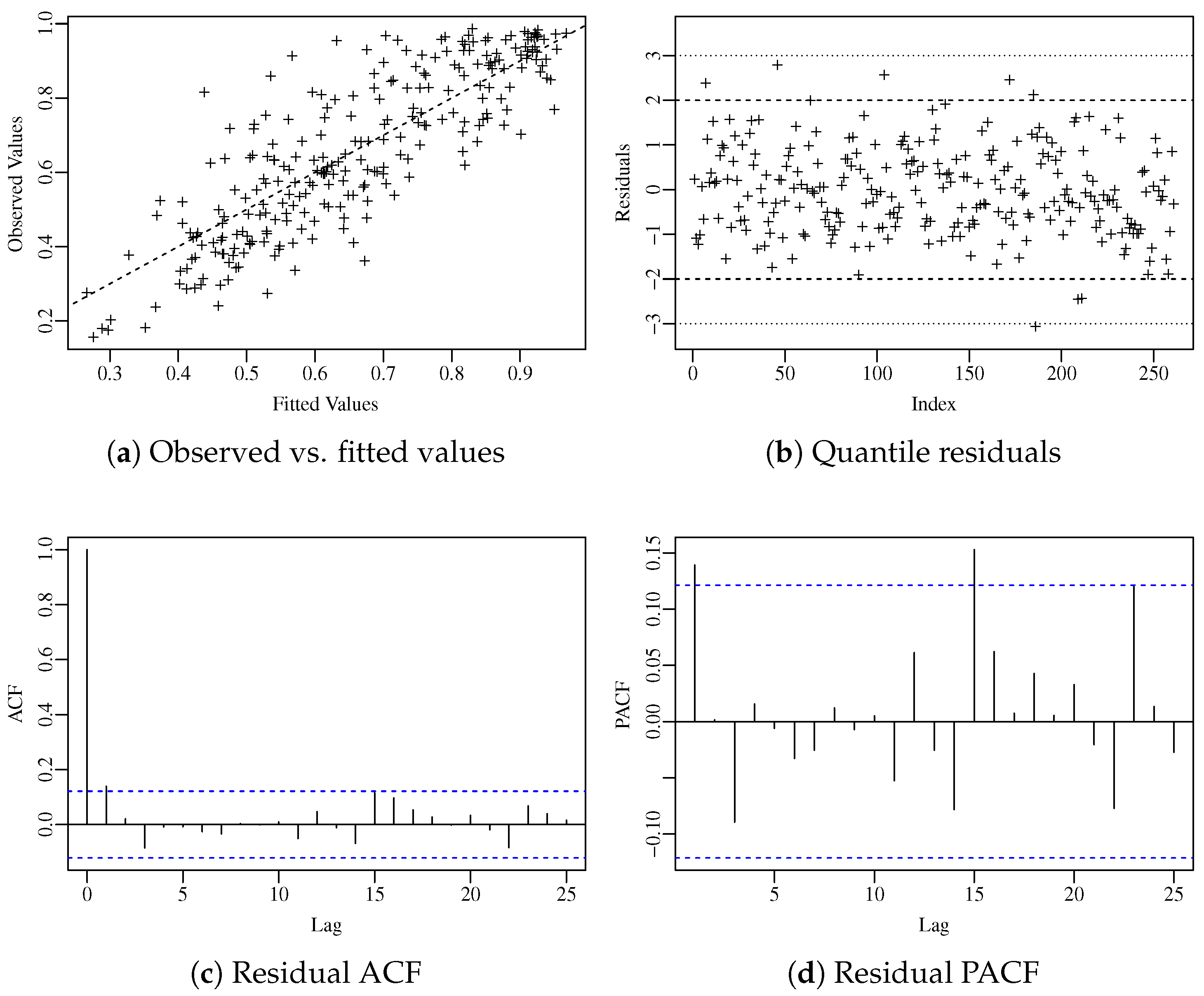
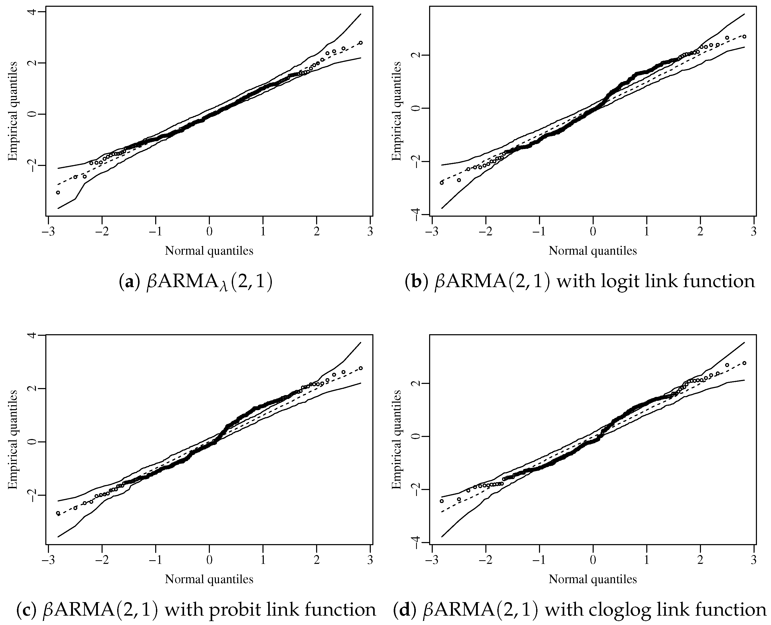
To carry on the residual analysis, we consider the standardized ordinary residual. The diagnostic plots presented in Figure 3 suggest that the residuals do not exhibit any pattern and are uncorrelated, as confirmed by the Ljung–Box test [13]. Figure 4 shows the normal plot with simulated envelope of the residuals considering the proposed model and the standard $\beta$ARMA model with different fixed link functions. Among all competitors, the proposed model was the only one capable of fitting the data adequately, with the residuals lying uniformly within the $95\%$ confidence region. The plots and tests further support the hypothesis that the model is correctly specified.

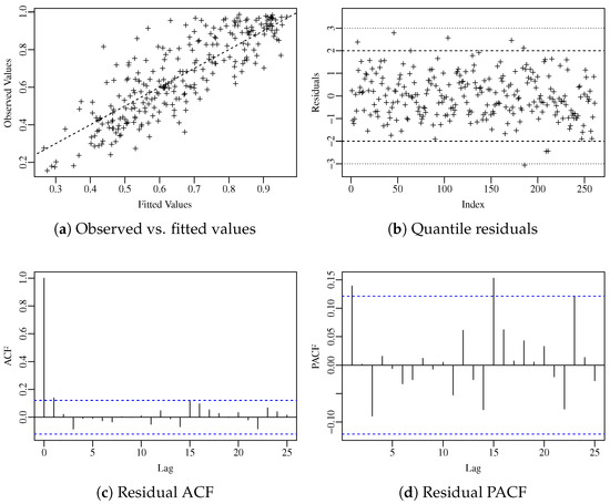
Figure 3. Diagnostic plots for the $\beta {\mathrm{ARMA}}_{\lambda }$$(2,1)$ residuals.

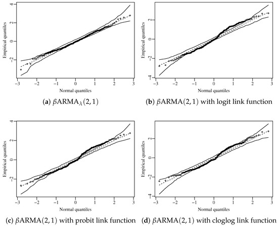
Figure 4. Normal plot with simulated envelope for different fitted models.

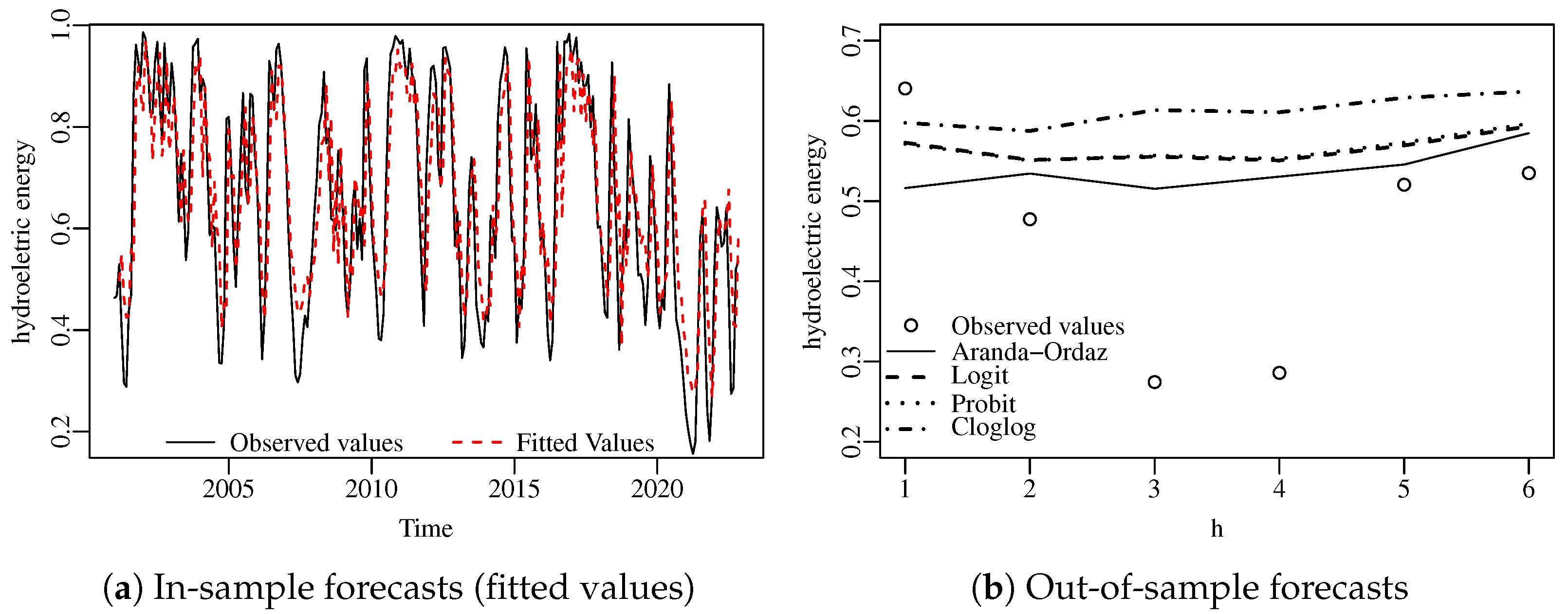
Figure 5a presents the time series plot of the data and the predicted values (in-sample forecasts), while Figure 5b presents the six-step out-of-sample forecasts. In order to make a comparison, we have added to the plot out-of-sample forecasts for the fitted $\beta$ARMA$(2,1)$ model coupled with four different link functions, namely, the fitted Aranda-Ordaz ($\beta {\mathrm{ARMA}}_{\lambda }$), the logit, the probit, and the cloglog. It is noteworthy that the $\beta {\mathrm{ARMA}}_{\lambda }$ model yielded more accurate out-of-sample forecasts than the competitors.

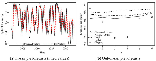
Figure 5. Observed in-sample and out-of-sample forecasts for the hydroelectric energy data.

Table 6 presents in-sample and out-of-sample forecasting root mean square error (RMSE), mean absolute error (MAE), and mean absolute percentage error (MAPE) measures between observed $y_t$ and fitted ${\widehat{\mu }}_t$ values, for all t, for the four fitted models. In addition, we present the forecast measures by modeling the time series with smaller periods, namely $n\in \left\{253,243,233\right\}$. We observe that the proposed $\beta {\mathrm{ARMA}}_{\lambda }$ model outperforms the competitor models in all metrics in the in-sample case. Considering out-of-sample forecasting, the proposed model outperforms in most cases, with lower performance only in MAPE for the logit and probit link functions, and in RMSE for the logit link function when considering $n=233$. The usual logit link function performs better than our proposal only in two metrics of one prediction scenario. Our proposal performs better in most cases, and when it does not, it is still very competitive. The Aranda-Ordaz link function with $\lambda =1.920$ has a heavier right tail compared to the other links, which may explain its superior forecasting performance.

Table 6. In-sample and out-of-sample ($h=6$) forecasting measures for the $\beta {\mathrm{ARMA}}_{\lambda }$$(2,1)$ model compared to the $\beta$ARMA model with other fixed links (best figures are in bold).

Link	In-Sample			Out-of-Sample
	RMSE	MAE	MAPE	RMSE	MAE	MAPE
$n=263$
Aranda-Ordaz	0.116	0.092	17.026%	0.153	0.124	36.474%
logit	0.155	0.130	24.395%	0.166	0.132	40.233%
probit	0.145	0.121	22.466%	0.167	0.134	40.676%
cloglog	0.145	0.122	22.899%	0.207	0.171	51.138%
$n=253$
Aranda-Ordaz	0.116	0.093	16.871%	0.103	0.073	13.384%
logit	0.155	0.130	24.082%	0.113	0.088	15.619%
probit	0.144	0.121	22.246%	0.107	0.081	14.539%
cloglog	0.146	0.125	23.755%	0.109	0.083	15.225%
$n=243$
Aranda-Ordaz	0.115	0.092	15.976%	0.183	0.157	59.158%
logit	0.152	0.129	22.349%	0.198	0.174	69.918%
probit	0.142	0.121	20.768%	0.186	0.160	64.178%
cloglog	0.142	0.121	21.130%	0.185	0.158	63.833%
$n=233$
Aranda-Ordaz	0.114	0.092	15.372%	0.265	0.233	53.918%
logit	0.150	0.128	21.526%	0.263	0.239	52.931%
probit	0.140	0.119	19.820%	0.267	0.240	53.906%
cloglog	0.140	0.120	20.008%	0.268	0.241	54.016%

Moreover, besides presenting the best forecast performance, the flexibility of the Aranda-Ordaz link allows for the proposed $\beta {\mathrm{ARMA}}_{\lambda }$ model to circumvent problems steaming from link function misspecification, being more robust and facilitating the construction of an adequate model for practitioners.

7. Conclusions

In this work, we considered an alternative way to model bounded time series by extending the relationship between the random component and linear predictors in the context of $\beta$ARMA models. To do that, we introduced the Aranda-Ordaz parametric link function in place of the traditional fixed links. The parameter on the Aranda-Ordaz link is estimated along the other $\beta$ARMA parameters by partial maximum likelihood. We discussed large sample inferences and presented a Monte Carlo simulation study showcasing the estimator’s performance in finite sample sizes. Based on the proposed methodology, we discussed residual analysis, hypothesis testing, and forecasting. Finally, a real data application to the proportion of stocked hydroelectric energy in the south of Brazil was presented, showcasing the usefulness of the proposed model, which has outperformed the competing ones.

References

- McKenzie, E. Some simple models for discrete variate time series. J. Am. Water Resour. Assoc. 1985, 21, 645–650. [Google Scholar] [CrossRef]
- McCullagh, P.; Nelder, J. Generalized Linear Models, 2nd ed.; Chapman and Hall: Boca Raton, FL, USA, 1989. [Google Scholar]
- Benjamin, M.A.; Rigby, R.A.; Stasinopoulos, D.M. Generalized autoregressive moving average models. J. Am. Stat. Assoc. 2003, 98, 214–223. [Google Scholar] [CrossRef]
- Kedem, B.; Fokianos, K. Regression Models for Time Series Analysis; John Wiley & Sons: Hoboken, NJ, USA, 2005. [Google Scholar]
- Janacek, G.; Swift, A. A class of models for non-normal time series. J. Time Ser. Anal. 1990, 11, 19–31. [Google Scholar] [CrossRef]
- Tiku, M.L.; Wong, W.K.; Vaughan, D.C.; Bian, G. Time series models in non-normal situations: Symmetric innovations. J. Time Ser. Anal. 2000, 21, 571–596. [Google Scholar] [CrossRef]
- Jung, R.C.; Kukuk, M.; Liesenfeld, R. Time series of count data: Modeling, estimation and diagnostics. Comput. Stat. Data Anal. 2006, 51, 2350–2364. [Google Scholar] [CrossRef]
- Ribeiro, T.F.; Peña-Ramírez, F.A.; Guerra, R.R.; Alencar, A.P.; Cordeiro, G.M. Forecasting the proportion of stored energy using the unit Burr XII quantile autoregressive moving average model. Comput. Appl. Math. 2024, 43, 27. [Google Scholar] [CrossRef]
- Ferrari, S.L.; Cribari-Neto, F. Beta regression for modelling rates and proportions. J. Appl. Stat. 2004, 31, 799–815. [Google Scholar] [CrossRef]
- Rocha, A.V.; Cribari-Neto, F. Beta autoregressive moving average models. TEST 2009, 18, 529, Erratum in TEST 2017, 26, 451–459. [Google Scholar] [CrossRef]
- Bayer, F.M.; Cintra, R.J.; Cribari-Neto, F. Beta seasonal autoregressive moving average models. J. Stat. Comput. Simul. 2018, 88, 2961–2981. [Google Scholar] [CrossRef]
- Pumi, G.; Valk, M.; Bisognin, C.; Bayer, F.M.; Prass, T.S. Beta autoregressive fractionally integrated moving average models. J. Stat. Plan. Inference 2019, 200, 196–212. [Google Scholar] [CrossRef]
- Scher, V.T.; Cribari-Neto, F.; Pumi, G.; Bayer, F.M. Goodness-of-fit tests for βARMA hydrological time series modeling. Environmetrics 2020, 31, e2607. [Google Scholar] [CrossRef]
- Palm, B.G.; Bayer, F.M.; Cintra, R.J. Prediction intervals in the beta autoregressive moving average model. Commun. Stat.-Simul. Comput. 2023, 52, 3635–3656. [Google Scholar] [CrossRef]
- Cribari-Neto, F.; Scher, V.T.; Bayer, F.M. Beta autoregressive moving average model selection with application to modeling and forecasting stored hydroelectric energy. Int. J. Forecast. 2023, 39, 98–109. [Google Scholar] [CrossRef]
- Bayer, F.M.; Pumi, G.; Pereira, T.L.; Souza, T.C. Inflated beta autoregressive moving average models. Comput. Appl. Math. 2023, 42, 183. [Google Scholar] [CrossRef]
- Czado, C. On selecting parametric link transformation families in generalized linear models. J. Stat. Plan. Inference 1997, 61, 125–140. [Google Scholar] [CrossRef]
- Guerrero, V.M.; Johnson, R.A. Use of the Box-Cox transformation with binary response models. Biometrika 1982, 69, 309–314. [Google Scholar] [CrossRef]
- Czado, C. Parametric link modification of both tails in binary regression. Stat. Pap. 1994, 35, 189–201. [Google Scholar] [CrossRef]
- Mallick, B.K.; Gelfand, A.E. Generalized Linear Models with Unknown Link Functions. Biometrika 1994, 81, 237–245. [Google Scholar] [CrossRef]
- Newton, M.A.; Czado, C.; Chappell, R. Bayesian Inference for Semiparametric Binary Regression. J. Am. Stat. Assoc. 1996, 91, 142–153. [Google Scholar] [CrossRef]
- Muggeo, V.M.; Ferrara, G. Fitting generalized linear models with unspecified link function: A P-spline approach. Comput. Stat. Data Anal. 2008, 52, 2529–2537. [Google Scholar] [CrossRef]
- Canterle, D.R.; Bayer, F.M. Variable dispersion beta regressions with parametric link functions. Stat. Pap. 2019, 60, 1541–1567. [Google Scholar] [CrossRef]
- Pumi, G.; Rauber, C.; Bayer, F.M. Kumaraswamy regression model with Aranda-Ordaz link function. TEST 2020, 29, 1051–1071. [Google Scholar] [CrossRef]
- Aranda-Ordaz, F.J. On two families of transformations to additivity for binary response data. Biometrika 1981, 68, 357–363. [Google Scholar] [CrossRef]
- Koenker, R.; Yoon, J. Parametric links for binary choice models: A Fisherian–Bayesian colloquy. J. Econom. 2009, 152, 120–130. [Google Scholar] [CrossRef]
- Ramalho, E.A.; Ramalho, J.J.; Murteira, J.M. Alternative estimating and testing empirical strategies for fractional regression models. J. Econ. Surv. 2011, 25, 19–68. [Google Scholar] [CrossRef]
- Flach, N. Generalized Linear Models with Parametric Link Families in R. Ph.D. Thesis, Department of Mathematics, Technische Universität München, München, Germany, 2014. [Google Scholar]
- Dehbi, H.M.; Cortina-Borja, M.; Geraci, M. Aranda-Ordaz quantile regression for student performance assessment. J. Appl. Stat. 2016, 43, 58–71. [Google Scholar] [CrossRef]
- Bayer, F.M.; Bayer, D.M.; Pumi, G. Kumaraswamy autoregressive moving average models for double bounded environmental data. J. Hydrol. 2017, 555, 385–396. [Google Scholar] [CrossRef]
- Nocedal, J.; Wright, S. Numerical Optimization; Springer: New York, NY, USA, 1999. [Google Scholar]
- Fahrmeir, L.; Kaufmann, H. Consistency and asymptotic normality of the maximum likelihood estimator in generalized linear models. Ann. Stat. 1985, 13, 342–368. [Google Scholar] [CrossRef]
- Czado, C.; Munk, A. Noncanonical links in generalized linear models—When is the effort justified? J. Stat. Plan. Inference 2000, 87, 317–345. [Google Scholar] [CrossRef]
- Fokianos, K.; Kedem, B. Partial likelihood inference for time series following generalized linear models. J. Time Ser. Anal. 2004, 25, 173–197. [Google Scholar] [CrossRef]
- Fokianos, K.; Kedem, B. Prediction and Classification of non-stationary categorical time series. J. Multivar. Anal. 1998, 67, 277–296. [Google Scholar] [CrossRef]
- Pawitan, Y. In All Likelihood: Statistical Modelling and Inference Using Likelihood; Oxford University Press: Oxford, UK, 2001. [Google Scholar]
- Wald, A. Tests of statistical hypotheses concerning several parameters when the number of observations is large. Trans. Am. Math. Soc. 1943, 54, 426–482. [Google Scholar] [CrossRef]
- Neyman, J.; Pearson, E.S. On the use and interpretation of certain test criteria for purposes of statistical inference: Part I. Biometrika 1928, 20, 175–240. [Google Scholar]
- Rao, C.R. Large sample tests of statistical hypotheses concerning several parameters with applications to problems of estimation. Math. Proc. Camb. Philos. Soc. 1948, 44, 50–57. [Google Scholar]
- Terrell, G.R. The gradient statistic. Comput. Sci. Stat. 2002, 34, 206–215. [Google Scholar]
- Akaike, H. A new look at the statistical model identification. IEEE Trans. Autom. Control 1974, 19, 716–723. [Google Scholar] [CrossRef]
- Schwarz, G. Estimating the dimension of a model. Ann. Stat. 1978, 6, 461–464. [Google Scholar] [CrossRef]
- Dunn, P.K.; Smyth, G.K. Randomized quantile residuals. J. Comput. Graph. Stat. 1996, 5, 236–244. [Google Scholar] [CrossRef]
- R Core Team. R: A Language and Environment for Statistical Computing; R Foundation for Statistical Computing: Vienna, Austria, 2018. [Google Scholar]
- Ospina, R.; Cribari-Neto, F.; Vasconcellos, K.L.P. Improved point and intervalar estimation for a beta regression model. Comput. Stat. Data Anal. 2006, 51, 960–981. [Google Scholar] [CrossRef]
- Box, G.E.; Jenkins, G.M.; Reinsel, G.C.; Ljung, G.M. Time Series Analysis: Forecasting and Control; John Wiley & Sons: Hoboken, NJ, USA, 2015. [Google Scholar]
Disclaimer/Publisher’s Note: The statements, opinions and data contained in all publications are solely those of the individual author(s) and contributor(s) and not of MDPI and/or the editor(s). MDPI and/or the editor(s) disclaim responsibility for any injury to people or property resulting from any ideas, methods, instructions or products referred to in the content. |
© 2024 by the authors. Licensee MDPI, Basel, Switzerland. This article is an open access article distributed under the terms and conditions of the Creative Commons Attribution (CC BY) license (https://creativecommons.org/licenses/by/4.0/).