Abstract
The dynamical analysis of Kurchatov’s scheme is extended to Traub’s method. The difference here is that Traub’s method requires two additional starting points. Therefore, the map is three-dimensional instead of 2-D. We obtain a complete description of the dynamical planes and show that the method is stable for cubic polynomials.
MSC:
65H05; 37D99
1. Introduction
The solution to a single nonlinear equation,
can be found in applied science and engineering. For example, the Colebrook equation [1] is used to find the friction factor. Most numerical solution methods are based on Newton’s scheme; i.e., starting with an initial guess for the root , we create a sequence :
The convergence is quadratic, that is,
To increase the order of convergence, p, one has to include higher derivatives, such as in Halley’s scheme [2], using first and second derivatives to achieve cubic convergence. In order to avoid higher derivatives, one can use multipoint methods; see, e.g., Traub [3] or Petković et al. [4].
Derivative-free one-step methods are either linear (such as Picard), superlinear (such as secant), or even quadratic, such as Steffensen’s method [5] or Kurchatov [6,7]. Clearly, we can construct multipoint methods that are derivative-free. Most of those are based on Steffensen’s method to achieve the highest possible order for the least number of function evaluations; see, for example, the fourth-order derivative-free methods in [8,9].
In a recent article, Neta [10] shows that there is a better choice for a first step, even though it is NOT second order. Traub’s method [3], given by
is of the order 1.839, and it runs faster and has better dynamics than several other derivative-free methods; see Neta [11], where several methods were compared to solve the discretized nonlinear diffusion model with source terms. Clearly, one cannot obtain optimal methods (see Kung and Traub [12]) this way. Kung and Traub [12] conjectured that multipoint methods without memory using d function evaluations could have an order no larger than . The efficiency index I is defined as . Thus, an optimal method of the order has an efficiency index of , and an optimal method of the order has an efficiency index of , which is better than Newton’s method for which . The efficiency index of the optimal method cannot reach a value of 2. In fact, realistically, one uses methods of the order 8 at most. For high-order derivative-free methods based on Steffensen’s method as the first step, see Zhanlav and Otgondorj [13] and references there. Such methods are especially useful when the derivative is very expensive to evaluate and, of course, when the function is nondifferentiable.
If we denote and , then the Traub algorithm can be studied from a dynamical point of view as a three-dimensional map:
Our study extends the results of Garijo and Jarque [14] for the secant method and of Campos et al. [7] for Kurchatov’s scheme. Both methods require only one memory point.
For the cubic polynomial
the map becomes
where
and
The set of nondefinition of is given by
Let
Points in define a natural subset of , where all iterates of are well defined, and so defines a smooth dynamical system.
The surface is a quadric surface. In general, a quadric surface [15] is given by
By means of rotation and translation, we can obtain one of these forms:
In our case, , and . If we take the following transformation to a new coordinate system :
we obtain three equations for the unknown whose solution is , and the surface becomes
Now we perform a translation to move the origin:
The equation becomes
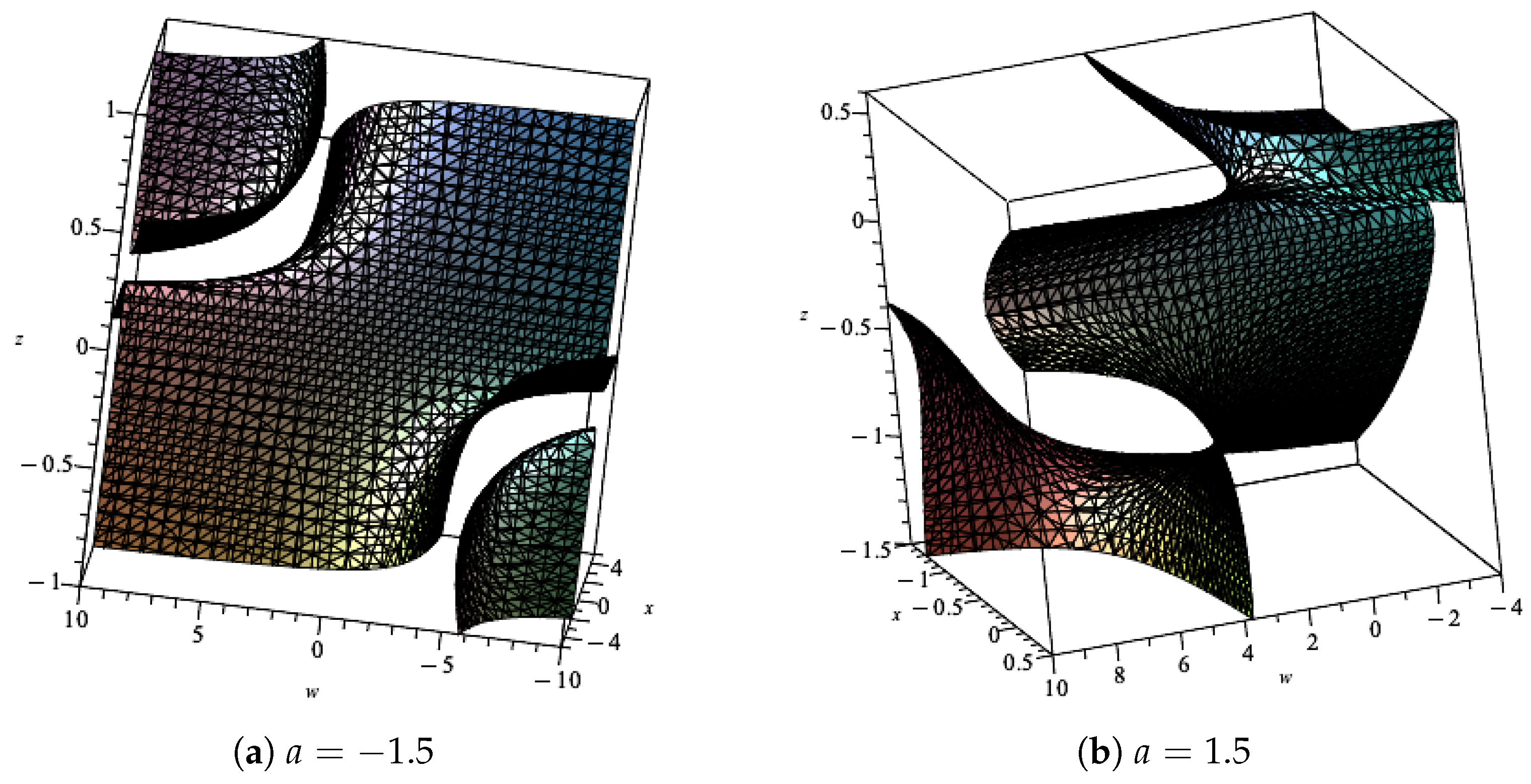
This surface is a hyperboloid of one sheet. The axis of symmetry is the axis. The trace of the surface can be obtained by taking as constant. If , then the equation of the trace is
This is a circle centered at . The radius is
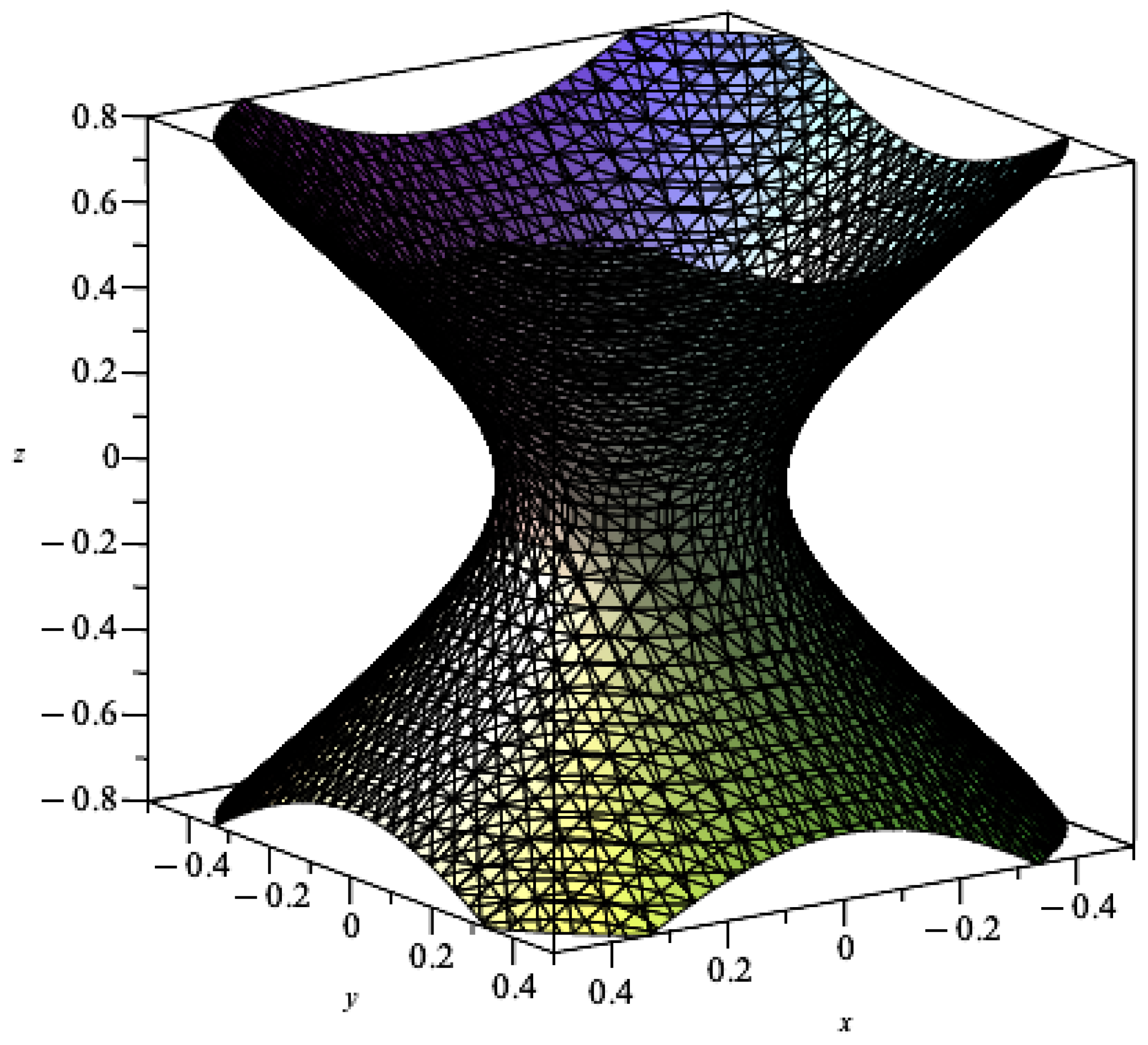
Clearly, the minimum value of the radius is when and . At that point, the radius is ; see Figure 1, Figure 2 and Figure 3.
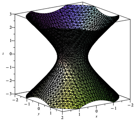
Figure 1.
Surface on which for The minimum value of the radius is .
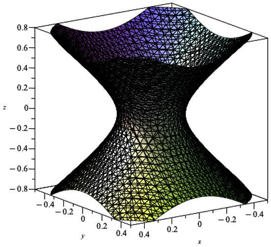
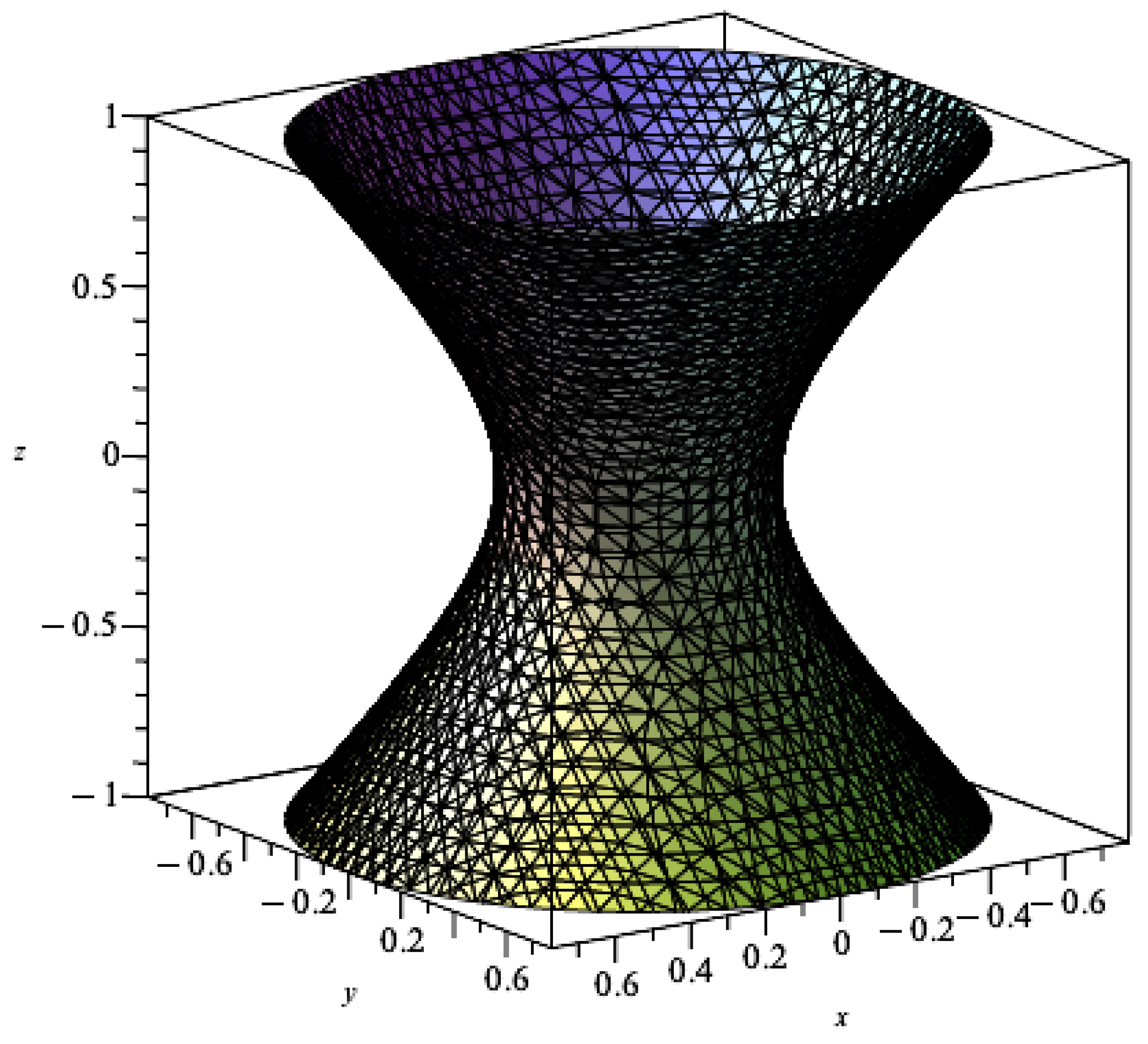
Figure 2.
Surface on which for The minimum value of the radius is .
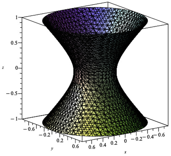
Figure 3.
Surface on which for The minimum value of the radius is .
Plotting the surface (10) (see Figure 1, Figure 2 and Figure 3), we see a hyperboloid of one sheet for three different values of a. Notice how the radius changes as a function of the value of a.
The origin in the coordinate system corresponds to
If , then both (8) and (9) vanish. The limit as x tending toward zero is zero, since the numerator is a polynomial in x of a degree higher than the denominator. This is called a focal point. A focal point Q is called simple if the tangent planes to the surfaces N and D are not parallel. This can be expressed by the condition
We now evaluate the gradient of the surfaces and at
Evaluating the derivatives at and then substituting in (18), we have
The surface can be described as follows: If (on the coordinate plane), we have the hyperbola If (a slanted plane through the w coordinate axis), then and w is free, that is, lines through the given points. Similarly, if , then and we have lines. If , we obtain the two points:
If again, we obtain a hyperbola:
If , then but Similarly, if or , If , then when , we can see if there is a point on the hyperbola (20) that will satisfy
Since and , we have the set of equations
Adding the two equation, we have
whose two solutions are and For we obtain For we obtain
The fixed points of the map,
are
or
One solution is , and the other two are the solution of
which are and . The fixed points coincide with the roots of .
In order to study their stability, we build the Jacobian matrix
where and the partial derivatives are
with
The partial derivatives at the roots are and
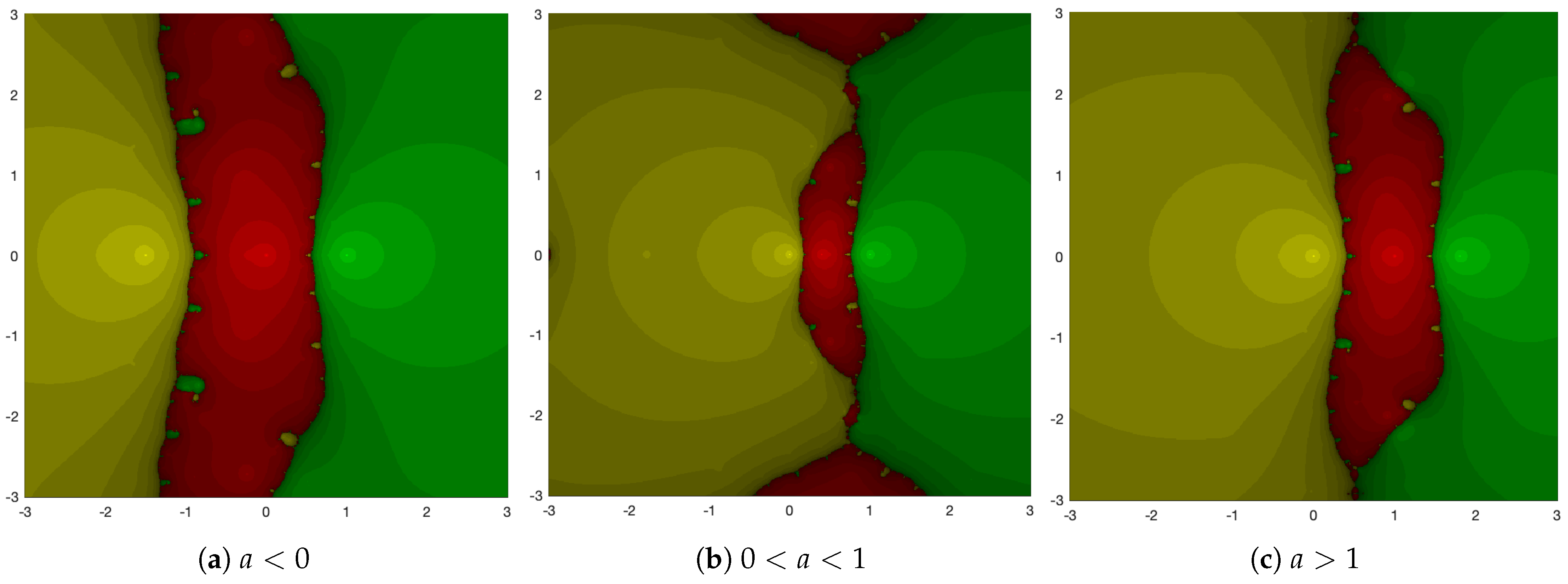
Therefore, the fixed points are attractive. In Figure 4, we plot the basins of attraction [16] of Traub’s method for the cubic polynomial (6) for three values of the parameter a, to the left of zero (), to the right of 1 (), and in between ().
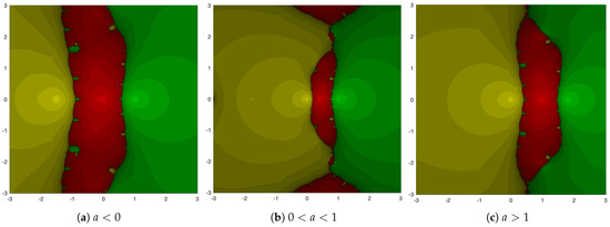
Figure 4.
Dynamical planes of Traub’s method for different values of the parameter a.
2. Dynamical Study of the Methods
Let us first analyze the curves or surfaces that are mapped on fixed points of the operator :
therefore, maps to the fixed point at the origin if and only if . On the other hand,
Therefore, . Finally,
then, and plane maps to its fixed points.
2.1. Focal Points and Prefocal Curves
Taking into account that focal points are those satisfying that at least one component is with finite limit, the focal points of satisfy
- also if ; then and replacing in (24), we obtain the surface in ,However, , so

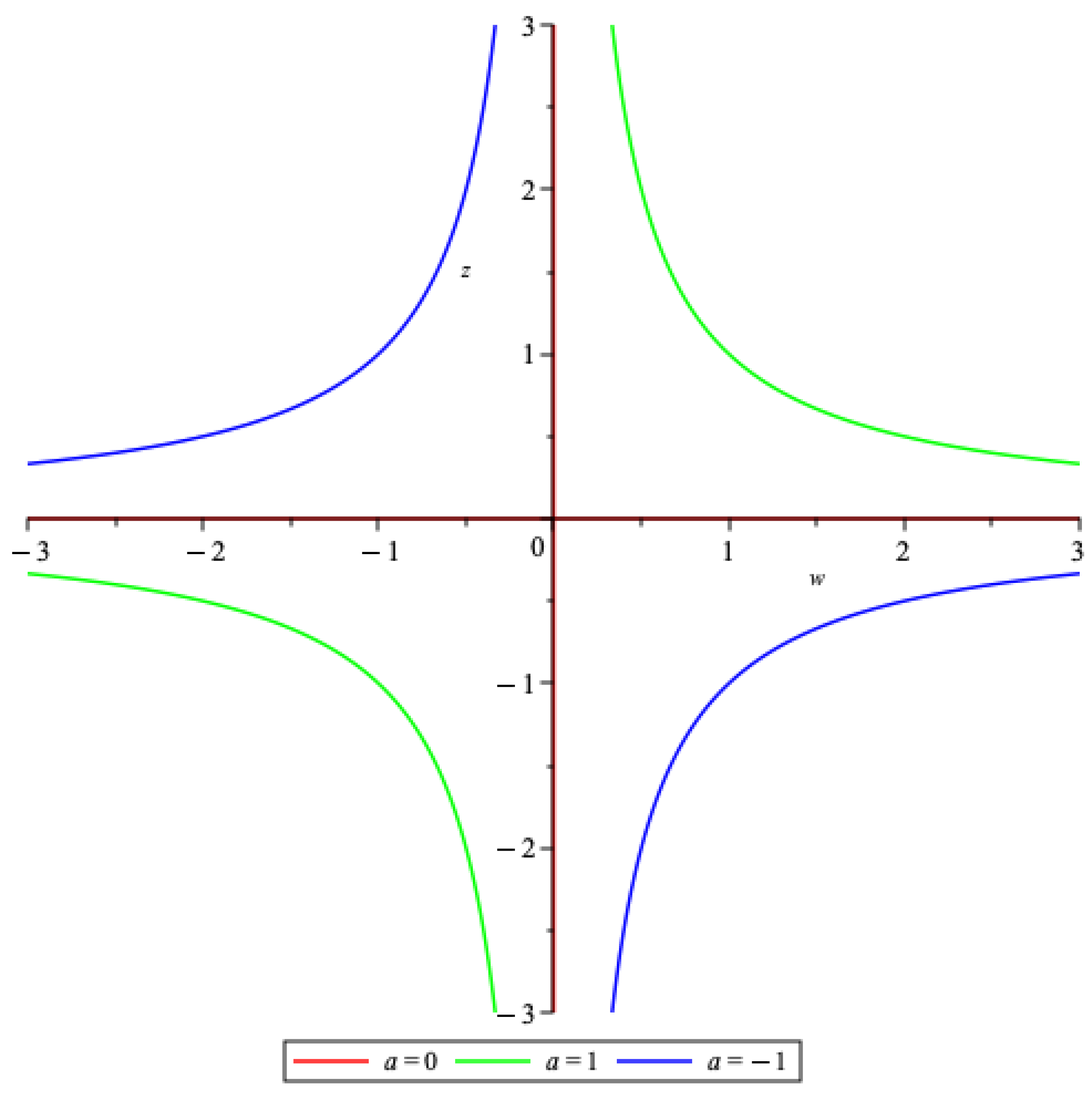
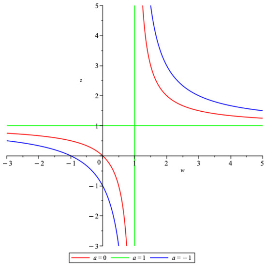
Figure 6.
Focal curve for for various values of a.
Figure 6.
Focal curve for for various values of a.

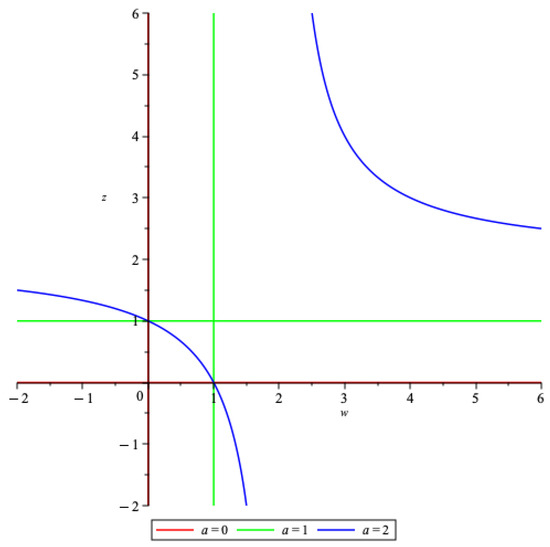
Figure 7.
Focal curve for for various values of a.
Figure 7.
Focal curve for for various values of a.

Thus, in all cases, the focal curve is a hyperbola. Notice that in Figure 7, we plot the cases that and . Those plots are just the asymptotes of the hyperbolas in Figure 5 and Figure 6.
To show that these points on the focal curves are all simple, we use (18)
We now look at the prefocal surface. A point Q in is a prefocal point if , the third component of (see (7)), evaluated at Q takes the form (i.e., ), and there exists a smooth simple arc , , with such that exists and it is finite. Moreover, the line , where is the first two components of . The line is the intersection of the two planes and evaluated at Q when . The equations of the line are
On , (for and ) and . Given on this hyperbola, we obtain , and the line for each is
The set of all these lines (for all possible on the focal curve) is the prefocal surface. This surface is a cylinder, and the lines are called rulings; see the definition in [15]. In Figure 8, we show the prefocal surface for a given a value.
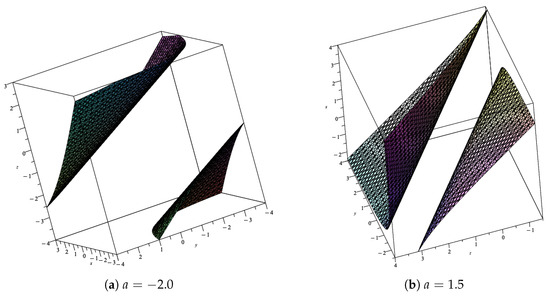
Figure 8.
Prefocal surfaces of Traub’s method for different values of the parameter a.
2.2. Inverse of Ta and Its Properties
In order to understand the global dynamics of the map , it is important to find the inverse map and in which regions of the phase space the inverse is defined. Let be a given point; then
The value of w is obtained by solving . We now look at the signs of the following three functions:
- 1.
- ;
- 2.
- ;
- 3.
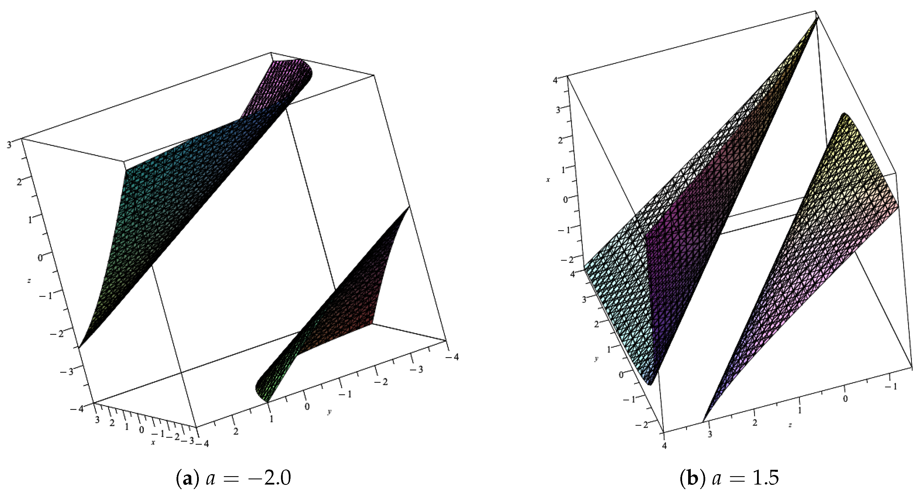
If all three or just one of them is positive, then ; otherwise, . The two planes and and the surface defined by the cubic are the boundaries of the regions. See Figure 9 for the surface defined by the cubic for two different values of the parameter a.

Figure 9.
One of the boundaries of the region for different values of the parameter a. The other two boundaries are the planes and .
The three surfaces meet at three possible points: the first is , and the other two solutions are given by solving the quadratic equation (using )
This equation has two complex roots as long as . For other values of a, the real roots are
Notice that unlike the secant [14] and Kurchatov’s [7] schemes, the solutions are not the three fixed points.
These surfaces form the boundary of the regions, but they are not a locus of critical points where the two inverses are defined and merged, since the denominator vanishes when . The locus is
Merging preimages are also in another set, denoted , that it is included in the set of points for which the determinant of the Jacobian vanishes, i.e., , or which is the same (see (22).) The set has critical points identical to the points of intersection of the boundaries above. In the case where , then w can take any value. In the case where z satisfies (29), then w satisfies the quadratic equation
3. Conclusions
The oldest method with memory is probably the secant method where one replaces the slope of the tangent line in Newton’s method by the slope of the secant. This, in turn, requires the use of an additional point besides the previous one. We generalize the analysis for two methods having one memory point (namely, the secant and Kurchatov’s schemes) to a method requiring two memory points. In this paper, we chose to study Traub’s method, which received a lot of attention recently. The analysis in three dimensions is not a trivial extension of the two-dimensional analysis in the literature. However, the generalization to methods using more than two memory points is relatively simple.
We have proved that Traub’s method is completely stable for any polynomial of the degree of 3 since the only attractors for any value of the parameter are the roots of the polynomial.
Funding
This research received no external funding.
Data Availability Statement
Data is contained within the article.
Acknowledgments
The author thanks Cordero for stimulating correspondence on the topic.
Conflicts of Interest
The author declares no conflict of interest.
References
- Colebrook, C.F. Turbulent flows in pipes, with particular reference to the transition between the smooth and rough pipe laws. J. Inst. Civ. Eng. 1938, 11, 130. [Google Scholar] [CrossRef]
- Halley, E. A new, exact and easy method of finding the roots of equations generally and that without any previous reduction. Philos. Trans. R. Soc. Lond 1694, 18, 136–148. [Google Scholar]
- Traub, J.F. Iterative Methods for the Solution of Equations; Prentice Hall: New York, NY, USA, 1964. [Google Scholar]
- Petković, M.S.; Neta, B.; Petković, L.D.; Džunić, J. Multipoint Methods for the Solution of Nonlinear Equations; Elsevier: Amsterdam, The Netherlands, 2012. [Google Scholar]
- Steffensen, J.F. Remarks on iteration. Scand. Actuar. J. 1933, 1, 64–72. [Google Scholar] [CrossRef]
- Kurchatov, V.A. On a method of linear interpolation for thew solution of functional equations (Russian). In Doklady Akademii Nauk; Russian Academy of Sciences: Moscow, Russia, 1971; Volume 198, pp. 524–526. [Google Scholar]
- Campos, B.; Cordero, A.; Torregrosa, J.R.; Vindel, P. Dynamical analysis of an iterative method with memory on a family of third-degree polynomials. AIMS Math. 2022, 7, 6445–6466. [Google Scholar] [CrossRef]
- Ren, H.; Wu, Q.; Bi, W. A class of two-step Steffensen type methods with fourth-order convergence. Appl. Math. Comput. 2009, 209, 206–210. [Google Scholar] [CrossRef]
- Sharma, J.R.; Arora, H. An efficient derivative-free iterative method for solving systems of nonlinear equations. Appl. Anal. Discret. Math. 2013, 7, 390–403. [Google Scholar] [CrossRef]
- Neta, B. Basin attractors for derivative-free methods to find simple roots of nonlinear equations. J. Numer. Anal. Approx. Theory 2020, 49, 177–189. [Google Scholar] [CrossRef]
- Neta, B. Comparison of several numerical solvers for a discretized nonlinear diffusion model with source terms. Georgian Math. J. 2023. Accepted for Publication. [Google Scholar] [CrossRef]
- Kung, H.T.; Traub, J.F. Optimal orderof one-point and multipoint iteration. J. Assoc. Comput. Math. 1974, 21, 634–651. [Google Scholar] [CrossRef]
- Zhanlav, T.; Otgondorj, K. Comparison of some optimal derivative-free three-point iterations. J. Numer. Anal. Approx. Theory 2020, 49, 76–90. [Google Scholar] [CrossRef]
- Garijo, A.; Jarque, X. Global dynamics of the real secant method. Nonlinearity 2019, 32, 4557–4578. [Google Scholar] [CrossRef]
- Stewart, J. Calculus, Early Transcendentals; Brooks/Cole: Pacific Grove, CA, USA, 1995. [Google Scholar]
- Stewart, B.D. Attractor Basins of Various Root-Finding Methods. Master’s Thesis, Naval Postgraduate School, Department of Applied Mathematics, Monterey, CA, USA, 2001. [Google Scholar]

Disclaimer/Publisher’s Note: The statements, opinions and data contained in all publications are solely those of the individual author(s) and contributor(s) and not of MDPI and/or the editor(s). MDPI and/or the editor(s) disclaim responsibility for any injury to people or property resulting from any ideas, methods, instructions or products referred to in the content. |
© 2024 by the author. Licensee MDPI, Basel, Switzerland. This article is an open access article distributed under the terms and conditions of the Creative Commons Attribution (CC BY) license (https://creativecommons.org/licenses/by/4.0/).