Real and Complex Potentials as Solutions to Planar Inverse Problem of Newtonian Dynamics

Abstract

We study the motion of a test particle in a conservative force field. In the framework of the 2D inverse problem of Newtonian dynamics, we find 2D potentials that produce a preassigned monoparametric family of regular orbits $f(x,y)=c$ on the $xy$-plane (where c is the parameter of the family of orbits). This family of orbits can be represented by the “slope function” $\gamma =\frac{f_y}{f_x}$ uniquely. A new methodology is applied to the basic equation of the planar inverse problem in order to find potentials of a special form, i.e., $V=F(x+y)+G(x-y)$, $V=F(x+iy)+G(x-iy)$ and $V=P\left(x\right)+Q\left(y\right)$, and polynomial ones. According to this methodology, we impose differential conditions on the family of orbits $f(x,y)$ = c. If they are satisfied, such a potential exists and it is found analytically. For known families of curves, e.g., circles, parabolas, hyperbolas, etc., we find potentials that are compatible with them. We offer pertinent examples that cover all the cases. The case of families of straight lines is referred to.

1. Introduction

The inverse problem of dynamics, as introduced by [1], seeks all the potentials $V(x,y)$ that can give rise to a monoparametric family of curves $f(x,y)$ = c, traced in the ($x,y$)-Cartesian plane by a material point of unit mass with any preassigned energy dependence $\mathcal{E}=\mathcal{E}\left(f\right)$. Since 1974, the interest in this problem has increased and Szebehely’s equation was studied by many authors (see [2,3,4]). An alternative form of Szebehely’s equation was given by [5] ten years later. This alternative form constitutes a linear second-order PDE in the unknown function $V=V(x,y)$, which relates the preassigned family of orbits $f(x,y)=c$ to the corresponding potential. Families of planar orbits produced by two-dimensional homogeneous potentials were studied by [6] and those produced by inhomogeneous potentials were examined by [7], respectively. Moreover, geometrically similar orbits produced by homogeneous potentials were studied in the paper by [8]. Family boundary curves were studied by [9] and the allowed region for the motion of the test particle was determined. A review on the basic facts of the inverse problem in dynamics was made by [10]. Other solvable cases of the planar inverse problem were produced by [11,12,13]. Studying the direct problem of Newtonian dynamics [14,15,16], the authors presented methodologies by which one can obtain monoparametric families of planar orbits if the potential $V=V(x,y)$ is given. Families of straight lines generated by planar potentials were also studied by [17]. Monoparametric families of orbits produced by two-dimensional integrable or non-integrable potentials were studied recently by [18].

In the present work, we address the following question: Given a monoparametric family of regular curves $f(x,y)$ = c, is there a potential $V=V(x,y)$ that produces this family of orbits? Thus, we select three categories of potentials:

(i)

Potentials that satisfy the two-dimensional wave equation, i.e., $V_{xx}-V_{yy}$ = 0.

(ii)

Potentials that satisfy the two-dimensional Laplace equation, i.e., $V_{xx}+V_{yy}$ = 0.

(iii)

Separable potentials of the from $V(x,y)=P\left(x\right)+Q\left(y\right)$, where $P,Q$ are arbitrary functions of the $C^2$-class, which satisfy the condition $V_{xy}=$ 0. They were used by [19].

(iv)

Polynomial potentials of the third degree, $V=a_{30}{x}^3+a_{21}{x}^{2}y+a_{12}x{y}^2+a_{03}{y}^3+a_{00}$.

This paper is organized as follows. In Section 2, we present the basic facts of the 2D inverse problem of dynamics. In Section 3, we develop a new methodology for finding potentials of the special form $V=F(x+y)+G(x-y)$, where $F,G$ are arbitrary functions of the $C^2$-class. These potentials are known from the bibliography and they satisfy the two-dimensional wave equation. In proceeding, we impose compatibility conditions on the orbital function $\gamma =\gamma (x,y)$, which is related to the given family of orbits. If these conditions are fulfilled, then we find such a potential by quadratures. In Section 4, we develop a methodology similar to the previous one for finding potentials of the special form $V=F(x+iy)+G(x-iy)$, where $F,G$ are arbitrary $C^2$-functions. These potentials are known from the bibliography because they satisfy the two-dimensional Laplace equation. More precisely, we again establish conditions for the orbital function $\gamma =\gamma (x,y)$. By using this methodology, one can find two- and one-dimensional potentials that produce the given family of orbits. In Section 5, we study potentials of the form $V=P\left(x\right)+Q\left(y\right)$ and we find a family of curves, e.g., circles and parabolas, produced by such potentials as orbits. Pertinent examples are given in each case. In Section 6, we take into account the polynomial potentials of the third degree and find suitable families of orbits that are compatible with them. In Section 7, we study a special category of curves on the $xy$-plane, i.e., families of straight lines, which are produced by the above potentials, and we draw some conclusions in Section 8.

2. The Mathematical Setup

We consider the monoparametric family of planar orbits

$$f(x,y)=c=const.$$

(1)

which is traced by a material point of the unit mass under the action of the potential $V=V(x,y)$. The total energy is constant. As it was shown by [5,6], the family of orbits (1) can be represented by the slope function

$$\gamma =\frac{f_y}{f_x},$$

(2)

and

$$\Gamma =\gamma {\gamma }_x-{\gamma }_y.$$

(3)

According to [5,6], the potential V = $V(x,y)$ has to satisfy one second-order linear PDE. For $\Gamma \ne$ 0, this PDE reads

$$-V_{xx}+\kappa V_{xy}+V_{yy}-(\lambda V_x+\mu V_y)=0,$$

(4)

where

$$\begin{array}{ccc}\hfill \kappa & =& \frac{1}{\gamma }-\gamma ,\lambda =\frac{1}{\Gamma }\left(-{\Gamma }_x+\frac{1}{\gamma }{\Gamma }_y\right),\hfill \\ \hfill \mu & =& \lambda \gamma +\frac{3\Gamma }{\gamma }.\hfill \end{array}$$

(5)

Here, the indices x, y stand for partial derivatives. There is a one-to-one correspondence between the slope function (2) and the family of orbits (1). This means that if the slope function $\gamma$ is given, then we can find the monoparametric family of orbits in the form (1) by solving analytically the ODE

$$\frac{dy}{dx}=-\frac{1}{\gamma }$$

(6)

The energy of the family of orbits (1) is found to be (p. 248, [14]):

$$\mathcal{E}=V-\frac{(1+{\gamma }^2)(V_x+\gamma V_y)}{2\Gamma }.$$

(7)

We note here that if $\Gamma$ = 0, the family of orbits consists of straight lines [17], and this case will be studied in Section 7.

3. The 2D Wave Equation

We consider the two-dimensional wave equation

$$V_{xx}-V_{yy}=0,$$

(8)

which is hyperbolic and has the general solution

$$V(x,y)=F(x+y)+G(x-y).$$

(9)

We note here that $F,G$ are arbitrary $C^2$-functions. We insert this expression for the potential into (4) and we find two conditions on the family of orbits (1).

Two Conditions on the Family of Orbits $f(x,y)=c$

We set $p=x+y,q=x-y$ and we find the derivatives of the first and second order of the potential function (9) with respect to $x,y$, respectively. We have:

$$V_x=F^{\prime }\left(p\right)+G^{\prime }\left(q\right),V_y=F^{\prime }\left(p\right)-G^{\prime }\left(q\right),$$

(10)

where $F^{\prime }\left(p\right)=\frac{dF}{dp}$, $G^{\prime }\left(q\right)=\frac{dG}{dq}$ and

$$\begin{array}{ccc}\hfill V_{xx}& =& F^{″}\left(p\right)+G^{″}\left(q\right),V_{xy}=F^{″}\left(p\right)-G^{″}\left(q\right),\hfill \\ \hfill V_{yy}& =& F^{″}\left(p\right)+G^{″}\left(q\right).\hfill \end{array}$$

(11)

Inserting them into Equation (4), we obtain the relation

$$\kappa F^{″}\left(p\right)-(\lambda +\mu )F^{\prime }\left(p\right)=\kappa G^{″}\left(q\right)+(\lambda -\mu )G^{\prime }\left(q\right).$$

(12)

For $\kappa \ne$ 0, we obtain from (12)

$$F^{″}\left(p\right)+{\nu }_1(x,y)F^{\prime }\left(p\right)=G^{″}\left(q\right)+{\nu }_2(x,y)G^{\prime }\left(q\right),$$

(13)

where ${\nu }_1=-\frac{\lambda +\mu }{\kappa }$ and ${\nu }_2=\frac{\lambda -\mu }{\kappa }$. Now, we observe that the function F depends only on the argument $p=x+y$ and the function G depends only on the argument $q=x-y$. In order to obtain a solution to our problem, the coefficients ${\nu }_1,{\nu }_2$ in (13) must have the same properties, i.e.,

$${\nu }_1(x,y)={\nu }_1(x+y),{\nu }_2(x,y)={\nu }_2(x-y).$$

(14)

In doing so, we reconsider the Equation (13) and we set

$$F^{″}\left(p\right)+{\nu }_1\left(p\right)F^{\prime }\left(p\right)=G^{″}\left(q\right)+{\nu }_2\left(q\right)G^{\prime }\left(q\right)=d_0=const.$$

(15)

We solve analytically each part of the relation (15). As a first step, we set $F^{\prime }\left(p\right)=H\left(p\right)$ and we obtain

$$H^{\prime }\left(p\right)+{\nu }_1\left(p\right)H\left(p\right)=d_0.$$

(16)

We apply the multiplier $I_1\left(p\right)=\int e^{\int {\nu }_1\left(p\right)dp}$ to the O.D.E (16) and we obtain

$$I_1\left(p\right)H^{\prime }\left(p\right)+{\nu }_1\left(p\right)I_1\left(p\right)H\left(p\right)=d_0{I}_1\left(p\right),$$

(17)

or, equivalently,

$${\left(I_1\left(p\right)H\left(p\right)\right)}^{\prime }=d_0{I}_1\left(p\right).$$

(18)

Now, we integrate (18) and we obtain

$$I_1\left(p\right)H\left(p\right)=d_0\int I_1\left(p\right)dp+d_1,d_1=const.$$

(19)

For $I_1\left(p\right)\ne$ 0, we divide each part of Equation (19) by the factor $I_1\left(p\right)$ and we find

$$H\left(p\right)=\left[d_0\int I_1\left(p\right)dp+d_1\right]I_2\left(p\right),I_2\left(p\right)=\frac{1}{I_1\left(p\right)}=e^{-\int {\nu }_1\left(p\right)dp},$$

(20)

or, equivalently,

$$H\left(p\right)=\left[d_0\int e^{\int {\nu }_1\left(p\right)dp}dp+d_1\right]e^{-\int {\nu }_1\left(p\right)dp},d_1=const.$$

(21)

The differential conditions (14) are the differential conditions for the slope function $\gamma$, which, if they are satisfied, ensure the existence of a potential satisfying (8). On the other hand, we consider that the conditions (14) are satisfied by the slope function $\gamma$. Having determined $H\left(p\right)=F^{\prime }\left(p\right)\ne 0$, we obtain the function F from (21).

$$F\left(p\right)=\int H\left(p\right)dp+d_2,d_2=const.$$

(22)

Working in a similar way for the function $G=G\left(q\right)$, we find the result

$$G\left(p\right)=\int J\left(q\right)dq+d_4,d_4=const.,$$

(23)

where

$$J\left(q\right)=\left[d_0\int e^{\int {\nu }_2\left(q\right)dq}dq+d_3\right]e^{-\int {\nu }_2\left(q\right)dq},d_3=const.$$

(24)

As a conclusion, combining the results (22) and (23), we can find the potential function V by quadratures. Now, we can formulate the next one.

Proposition 1.

If the differential conditions (14) are satisfied for the given family of orbits (1), then a potential of the form V = $F\left(p\right)+G\left(q\right)$ always exists and it is determined uniquely from the relation $V(x,y)=F\left(p\right)+G\left(q\right)$ up to four arbitrary constants.

Example 1.

We study the monoparametric family of circles (see Figure 1a)

$$f(x,y)=x^2+y^2=c,$$

(25)

and

$$\gamma =\frac{y}{x},\Gamma =-\frac{x^2+y^2}{x^3}\ne 0.$$

(26)

Figure 1. (a) Some members of the family of orbits (25) for $c=1,4,9$ (closed curves). (b) Some members of the family of orbits (33) for $c=1,4,9$ (open curves).

Then, we estimate the quantities ${\nu }_1,{\nu }_2$ in (13). It is

$${\nu }_1(x,y)=\frac{3}{x+y}=\frac{3}{p},{\nu }_2(x,y)=\frac{3}{x-y}=\frac{3}{q}.$$

(27)

From (21), we find the function $H=H\left(p\right)$

$$H\left(p\right)=\frac{1}{4}{d}_{0}p+\frac{d_1}{p^3},$$

(28)

and from (22), we determine the function $F=F\left(p\right)$. The result is

$$F\left(p\right)=\frac{1}{8}{d}_0{p}^2-\frac{d_1}{2p^2}.$$

(29)

Working in a similar way, we find the function $J=J\left(q\right)$ from (24). It is

$$J\left(q\right)=\frac{1}{4}{d}_{0}q+\frac{d_3}{q^3},$$

(30)

and from (23), we estimate the function $G=G\left(q\right)$.

$$G\left(q\right)=\frac{1}{8}{d}_0{q}^2-\frac{d_3}{2q^2}.$$

(31)

Combining the results (29) and (31), we find the potential

$$V(x,y)=\frac{1}{4}{d}_0(x^2+y^2)-\frac{d_1}{2{(x+y)}^2}-\frac{d_3}{2{(x-y)}^2},$$

(32)

and the energy of the family of orbits (1) is found to be $\mathcal{E}=\frac{1}{2}{d}_{0}c$.

Example 2.

Consider the monoparametric family of hyperbolas (see Figure 1b)

$$f(x,y)=x^2-y^2=c,$$

(33)

and

$$\gamma =-\frac{y}{x},\Gamma =\frac{x^2-y^2}{x^3}\ne 0.$$

(34)

Then, we estimate the quantities ${\nu }_1,{\nu }_2$ in (13). It is

$${\nu }_1(x,y)=-\frac{3}{x+y}=-\frac{3}{p},{\nu }_2(x,y)=-\frac{3}{x-y}=-\frac{3}{q}.$$

(35)

From (16), we find the function $H=H\left(p\right)$

$$H\left(p\right)=-\frac{1}{2}{d}_{0}p+d_1{p}^3,$$

(36)

and from (22), we determine the function $F=F\left(p\right)$. The result is

$$F\left(p\right)=\frac{1}{4}(-d_0{p}^2+d_1{p}^4).$$

(37)

Working in a similar way, we find the function $J=J\left(q\right)$ from (24). It is

$$J\left(q\right)=-\frac{1}{2}{d}_{0}q+d_1{q}^3,$$

(38)

and from (23), we estimate the function $G=G\left(w\right)$.

$$G\left(q\right)=\frac{1}{4}(-d_0{q}^2+d_3{q}^4).$$

(39)

Combining the results (37) and (39), we find the potential

$$V(x,y)=\frac{1}{4}[-2d_0(x^2+y^2)+d_1{(x+y)}^4+d_3{(x-y)}^4],$$

(40)

which is a polynomial of the fourth degree, and the energy of the family of orbits (1) is found to be $\mathcal{E}=-\frac{1}{4}(d_1+d_3)c$.

4. The 2D Laplace Equation

We consider the two-dimensional Laplace equation

$$V_{xx}+V_{yy}=0,$$

(41)

which is elliptic and has the general solution

$$V(x,y)=F(x+iy)+G(x-iy),i^2=-1.$$

(42)

We note here that $F,G$ are arbitrary $C^2$-functions. Inserting this expression for the potential into (4), we find two conditions on the family of orbits (1). In this case, not only real but complex potentials are expected to be solutions to our problem.

Two Conditions on the Family of Orbits $f(x,y)=c$

We set $z=x+iy,w=\overline{z}=x-iy$ and we compute the derivatives of the first and second order of the potential function (42) with respect to $x,y$, respectively. We have:

$$V_x=F^{\prime }\left(z\right)+G^{\prime }\left(w\right),V_y=i(F^{\prime }\left(z\right)-G^{\prime }\left(w\right)),$$

(43)

where $F^{\prime }\left(z\right)=\frac{dF}{dz}$, $G^{\prime }\left(w\right)=\frac{dG}{dw}$ and

$$\begin{array}{ccc}\hfill V_{xx}& =& F^{″}\left(z\right)+G^{″}\left(w\right),V_{xy}=i(F^{″}\left(z\right)-G^{″}\left(w\right)),\hfill \\ \hfill V_{yy}& =& -(F^{″}\left(z\right)+G^{″}\left(w\right)),\hfill \end{array}$$

(44)

and we insert them into Equation (4). Thus, we obtain the next relation

$$(i\kappa -2)F^{″}\left(z\right)-(\lambda +i\mu )F^{\prime }\left(z\right)=(i\kappa +2)G^{″}\left(w\right)+(\lambda -i\mu )G^{\prime }\left(w\right).$$

(45)

If we set

$$\begin{array}{ccc}\hfill {\xi }_2& =& i\kappa -2,{\xi }_1=-(\lambda +i\mu ),\hfill \\ \hfill {\xi }_4& =& i\kappa +2,{\xi }_3=\lambda -i\mu ,\hfill \end{array}$$

(46)

then the relation (45) takes the form

$${\xi }_2(x,y)F^{″}\left(z\right)+{\xi }_1(x,y)F^{\prime }\left(z\right)={\xi }_4(x,y)G^{″}\left(w\right)+{\xi }_3(x,y)G^{\prime }\left(w\right),$$

(47)

From (47), we observe that the function F depends only on the argument $z=x+iy$ and the function G depends only on the argument $w=x-iy$. In order to have a solution to our problem, the coefficients ${\xi }_1,{\xi }_2,{\xi }_3,{\xi }_4$ in (47) must have the same properties, i.e.,

$$\begin{array}{ccc}\hfill {\xi }_1(x,y)& =& {\xi }_1(x+iy),{\xi }_2(x,y)={\xi }_2(x+iy),\hfill \\ \hfill {\xi }_3(x,y)& =& {\xi }_3(x-iy),{\xi }_4(x,y)={\xi }_4(x-iy).\hfill \end{array}$$

(48)

Since the slope function $\gamma$ appears implicitly in (46), we can develop a methodology for finding potentials of the form (42).

• 1. “Plan A”.
  If the conditions (48) are satisfied for the given family of orbits (1), then we reconsider the Equation (47) and we set

  $${\xi }_2\left(z\right)F^{″}\left(z\right)+{\xi }_1\left(z\right)F^{\prime }\left(z\right)={\xi }_4\left(w\right)G^{″}\left(w\right)+{\xi }_3\left(w\right)G^{\prime }\left(w\right)=d_0=const.$$

  (49)
  We solve analytically each part of the relations (49). First, taking into account ${\xi }_2\ne$ 0, we set $F^{\prime }\left(z\right)=H\left(z\right)$ and we obtain

  $$H^{\prime }\left(z\right)+{\nu }_1\left(z\right)H\left(z\right)=d_1\left(z\right),{\nu }_1\left(z\right)=\frac{{\xi }_1\left(z\right)}{{\xi }_2\left(z\right)},d_1\left(z\right)=\frac{d_0}{{\xi }_2\left(z\right)}$$

  (50)

  with the general solution

  $$H\left(z\right)=\left[{\int }_0^z{d}_1\left(z\right)e^{{\int }_0^z{\nu }_1\left(z\right)dz}dz+c_1\right]e^{-{\int }_0^z{\nu }_1\left(z\right)dz},c_1=const.$$

  (51)

  The differential conditions (48) are the differential conditions for the slope function $\gamma$, which, if they are satisfied, ensure the existence of a potential (41). On the other hand, we consider that the conditions (48) are satisfied by the slope function $\gamma$. Besides that, we have $F^{\prime }\left(z\right)\ne 0$. Then, we obtain $F=F\left(z\right)$ and we determine the function F from (52).

  $$F\left(z\right)={\int }_0^{z}H\left(z\right)dz+c_2,c_2=const.$$

  (52)

  Working in a similar way for the function $G=G\left(w\right)$, we set $G^{\prime }\left(w\right)=J\left(w\right)$ and, with the aid of (49), we obtain the O.D.E.

  $${\xi }_4\left(w\right)J^{\prime }\left(w\right)+{\xi }_3\left(w\right)J\left(w\right)=d_0,$$

  (53)

  or, equivalently, assuming ${\xi }_4\ne 0$,

  $$J^{\prime }\left(w\right)+{\nu }_2\left(w\right)J\left(w\right)=d_2\left(w\right),{\nu }_2\left(w\right)=\frac{{\xi }_3\left(w\right)}{{\xi }_4\left(w\right)},d_2\left(w\right)=\frac{d_0}{{\xi }_4\left(w\right)}.$$

  (54)

  The general solution of (54) is

  $$J\left(w\right)=\left[{\int }_0^w{d}_2\left(w\right)e^{{\int }_0^w{\nu }_2\left(w\right)dw}dw+c_3\right]e^{-{\int }_0^w{\nu }_2\left(w\right)dw},c_3=const.$$

  (55)

  Finally, the function $G=G\left(w\right)$ is found to be

  $$G\left(w\right)={\int }_0^{w}J\left(w\right)dw+c_4,c_4=const.$$

  (56)

  As a conclusion, combining the results (52) and (56), we can find the potential function V by quadratures, i.e., $V=F\left(z\right)+G\left(w\right)$. Now, we can formulate the next one.

  Proposition 2.

  If ${\xi }_2(x,y),{\xi }_4(x,y)\ne 0$ and the differential conditions (48) are satisfied for the given family of orbits (1), then a potential of the form V = $F\left(z\right)+G\left(w\right)$ always exists and it is determined uniquely from the relation $V(x,y)=F\left(z\right)+G\left(w\right)$ up to four arbitrary constants.
• 2. “Plan B”.
  If the conditions (48) are not satisfied for the given family of orbits (1), then we refer to the Equation (47) and we use “the method of the determination of coefficients”. More precisely, since the functions $F,G$ are twice differentiable, we consider that the functions $F\left(z\right),G\left(w\right)$ are polynomials of the second degree and we set

  $$F\left(z\right)=b_2{z}^2+b_{1}z+b_0,G\left(w\right)=d_2{w}^2+d_{1}z+d_0$$

  (57)

  where $b_2,b_1,b_0,d_2,d_1,d_0$ are const. Then, we are searching for suitable values of these parameters such that the relations (47) are satisfied.

Example 3.

We study the monoparametric family of orbits

$$f(x,y)=x{y}^i=c,i^2=-1,$$

(58)

and

$$\gamma =\frac{ix}{y},\Gamma =-\frac{(1-i)x}{y^2}\ne 0.$$

(59)

For the given orbital function γ, the conditions (48) are not satisfied; so, we proceed with Plan B. We consider the functions $F,G$ defined in Equation (57) and we insert them in (47). The relations (47) are satisfied if and only if

$$b_2=d_2,b_1=d_1=0.$$

(60)

Thus, the functions $F,G$ in (57) take the concise form

$$F\left(z\right)=d_2{(x+iy)}^2+b_0,G\left(w\right)=d_2{(x-iy)}^2+d_0,$$

(61)

and the potential function $V=V(x,y)$ is the following

$$V(x,y)=d_2(x^2-y^2)+b_0+d_0.$$

(62)

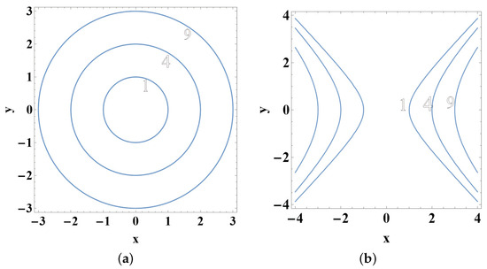
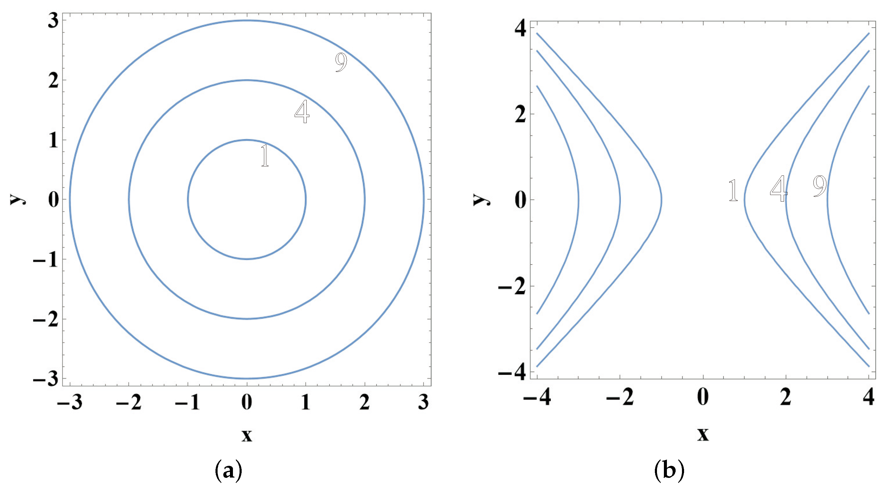
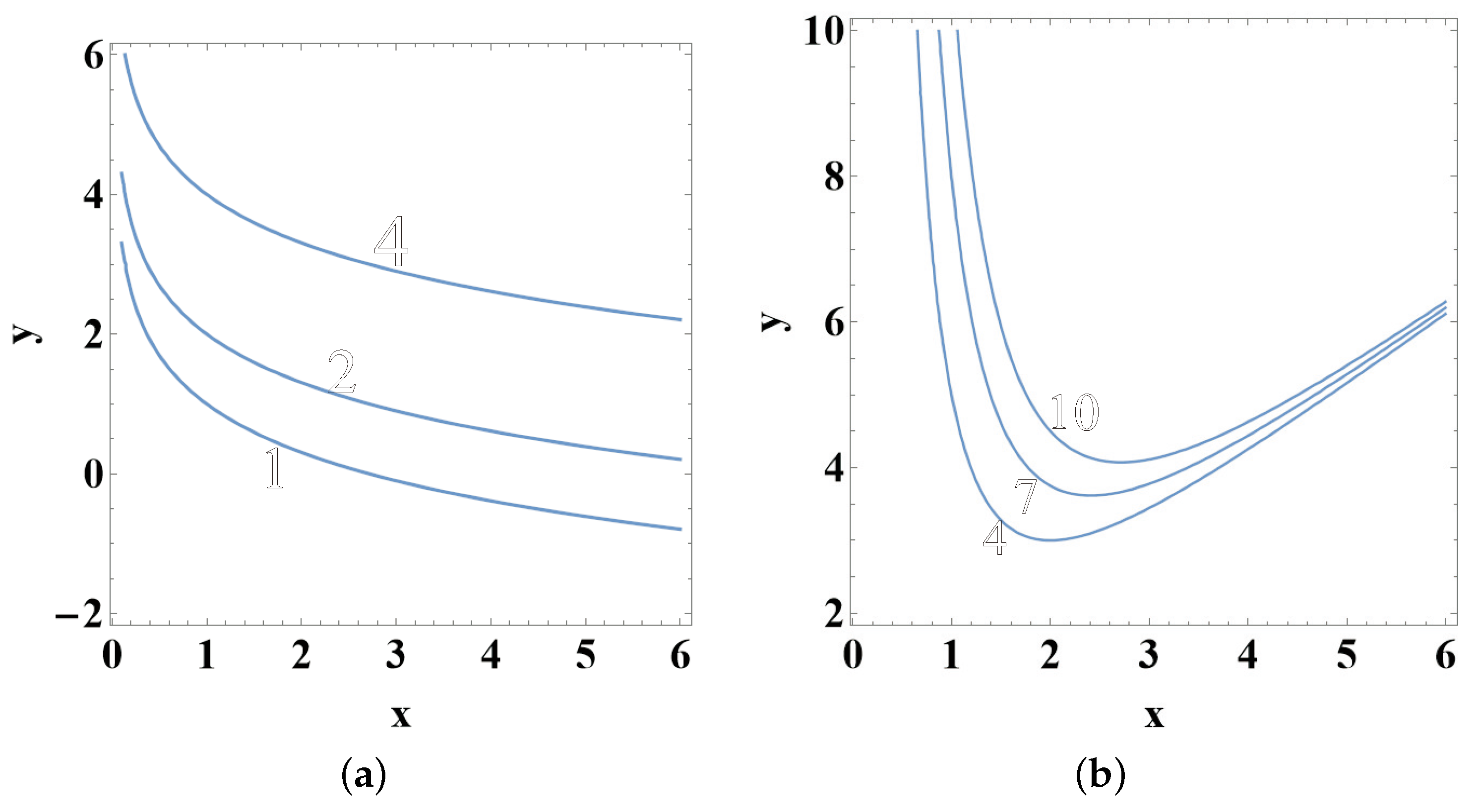
Thus, a real potential produces the family of orbits (58). The energy of this family of orbits is found to be $\mathcal{E}=b_0+d_0$ = const. Other results for families of orbits compatible with complex or real potentials are presented in Table 1.

Table 1. Families of orbits and potentials.

Family of Orbits	Potential V (x, y)	Energy
$f(x,y)=\frac{x}{y^2}=c$	$2d_{1}x+2$	$2-\frac{d_1}{2c}$
$f(x,y)=x+y^2=c$	$2(1+d_{1}x)$	$\frac{1}{2}(4+d_1+4d_{1}c)$
$f(x,y)=y+x^2=c$	$2(1-i{d}_{1}y)$	$-\frac{1}{2}i(4i+d_1+4d_{1}c)$
$f(x,y)=\frac{x}{\sqrt{y}}=c$	$2(1-i{d}_{1}y)$	$2+i{d}_1{c}^2$

5. Separable Potentials

In this section, we shall consider separable potentials in the $x,y$ coordinates, i.e., potentials of the form $V(x,y)=P\left(x\right)+Q\left(y\right)$, where $P,Q$ are arbitrary functions of the $C^2$-class. These potentials satisfy the condition $V_{xy}$ = 0 and they are used by [19] in the study of planar potentials with linear or quadratic invariants. Inserting this potential into (4), we obtain

$$P^{″}\left(x\right)+\lambda P^{\prime }\left(x\right)=Q^{″}\left(y\right)-\mu Q^{\prime }\left(y\right).$$

(63)

If $\lambda =\lambda \left(x\right)$ and $\mu =\mu \left(y\right)$, then we have a solution to our problem, otherwise not. In this case, the left hand of (63) is an expression that depends only on the argument x and the right hand of (63) is an expression of the argument y. Thus, we can set

$$P^{″}\left(x\right)+\lambda P^{\prime }\left(x\right)=Q^{″}\left(y\right)-\mu Q^{\prime }\left(y\right)=d_0=const.$$

(64)

We solve analytically each part of the relations (64). In the first step, we set $P^{\prime }\left(x\right)=R\left(x\right)$ and we obtain

$$R^{\prime }\left(x\right)+\lambda R\left(x\right)=d_0$$

(65)

with the general solution

$$R\left(x\right)=\left[d_0\int e^{\int \lambda \left(x\right)dx}dx+b_1\right]e^{-\int \lambda \left(x\right)dx},b_1=const.$$

(66)

Then, we find the function $P=P\left(x\right)$. It is:

$$P\left(x\right)=\int R\left(x\right)dx+b_2,b_2=const.$$

(67)

Working in a similar way, we find

$$Q\left(y\right)=\int S\left(y\right)dy+d_2,d_2=const.$$

(68)

where

$$S\left(y\right)=\left[d_0\int e^{-\int \mu \left(y\right)dy}dy+d_1\right]e^{\int \mu \left(y\right)dy},d_1=const.$$

(69)

Example 4.

We regard the monoparametric family of orbits (see Figure 2a)

$$f(x,y)=y+logx=c,$$

(70)

and

$$\gamma =x,\Gamma =x\ne 0.$$

(71)

Figure 2. (a) Some members of the family of orbits (70) for $c=1,2,4$. (b) Some members of the family of orbits (77) for $c=4,7,10$ and $b_0=-$1.

Then, we estimate the quantities $\kappa ,\lambda ,\mu$ in (5). It is

$$\kappa (x,y)=x-\frac{1}{x},\lambda (x,y)=-\frac{1}{x},\mu (x,y)=2.$$

(72)

From (67), we find the function $P=P\left(x\right)$

$$P\left(x\right)=-\frac{1}{4}{d}_0{x}^2+\frac{1}{2}{d}_0{x}^{2}logx+\frac{1}{2}{b}_1{x}^2+b_2,$$

(73)

and from (68), we determine the function $Q=Q\left(y\right)$. The result is

$$Q\left(y\right)=-\frac{1}{2}{d}_{0}y+\frac{1}{2}{d}_1{e}^y+d_2.$$

(74)

Adding the results (73) and (74), we find the potential function

$$V(x,y)=\frac{1}{4}[2d_1{e}^{2y}+2b_1{x}^2-d_0(x^2+2y-2x^{2}logx)]+j_2,j_2=b_2+d_2,$$

(75)

and the energy of the family of orbits (70) is found to be

$$\mathcal{E}=-\frac{1}{4}(2b_1-d_0+2d_{0}c+2d_1{e}^{2c})=const.$$

Other results are presented in Table 2.

Table 2. Families of orbits and potentials.

Family of Orbits	Potential V (x, y)	Energy
$f(x,y)=y+x^2=c$	$d_0(x^2+4y^2)-\frac{b_1}{2x^2}+d_{1}y$	$2b_1+d_1(\frac{1}{4}+c)+2d_0(c+2c^2)$
$f(x,y)=x+y^2=c$	$d_0(4x^2+y^2)+b_{1}x-\frac{d_1}{2y^2}$	$b_1(\frac{1}{4}+c)+2[d_1+d_0(c+2c^2)]$
$f(x,y)=x^2+y^2=c$	$d_0(x^2+y^2)-\frac{b_1}{2x^2}-\frac{d_1}{2y^2}$	$2d_{0}c$
$f(x,y)=x{y}^2=c$	$d_0(4x^2+y^2)+\frac{1}{6}(2b_1{x}^3+d_1{y}^6)$	$-\frac{1}{12}(b_1+8d_{1}c)$

6. Polynomial Potentials

In this paragraph, we shall deal with polynomial potentials of the third degree

$$V=a_{30}{x}^3+a_{21}{x}^{2}y+a_{12}x{y}^2+a_{03}{y}^3+a_{00},$$

(76)

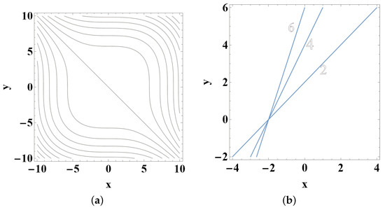
where $a_{30},a_{21},a_{12},a_{03},a_{00}$ are const. and they produce a bi-parametric family of orbits (see Figure 2b)

$$f(x,y)=b_0{x}^3+x^{2}y=c,b_0=const.\ne 0.$$

(77)

The potentials (76) do not have any special properties, but they were used mainly in the problem of integrability (see, e.g., [20]). Thus, we shall work only with Equation (4). We shall offer the following.

Example 5.

We consider the family of orbits (77) and the potential of the form (76). We insert it into (4) and we take the expression

$$q_1{x}^3+q_2{x}^{2}y+q_{3}x{y}^2+q_4{y}^3=0,$$

(78)

where

$$\begin{array}{ccc}\hfill q_1& =& 6(-a_{21}+a_{12}{b}_0+3a_{21}{b}_0^2),\hfill \\ \hfill q_2& =& 3(10a_{21}{b}_0+6(a_{30}+a_{03}{b}_0)+a_{12}(6b_0^2-2)),\hfill \\ \hfill q_3& =& 3(8a_{21}+10a_{12}{b}_0),\hfill \\ \hfill q_4& =& 18a_{12}.\hfill \end{array}$$

The last relation (78) must be identically zero. Thus, we have:

$$a_{12}=0,a_{21}=0,a_{30}=-a_{03}{b}_0.$$

(79)

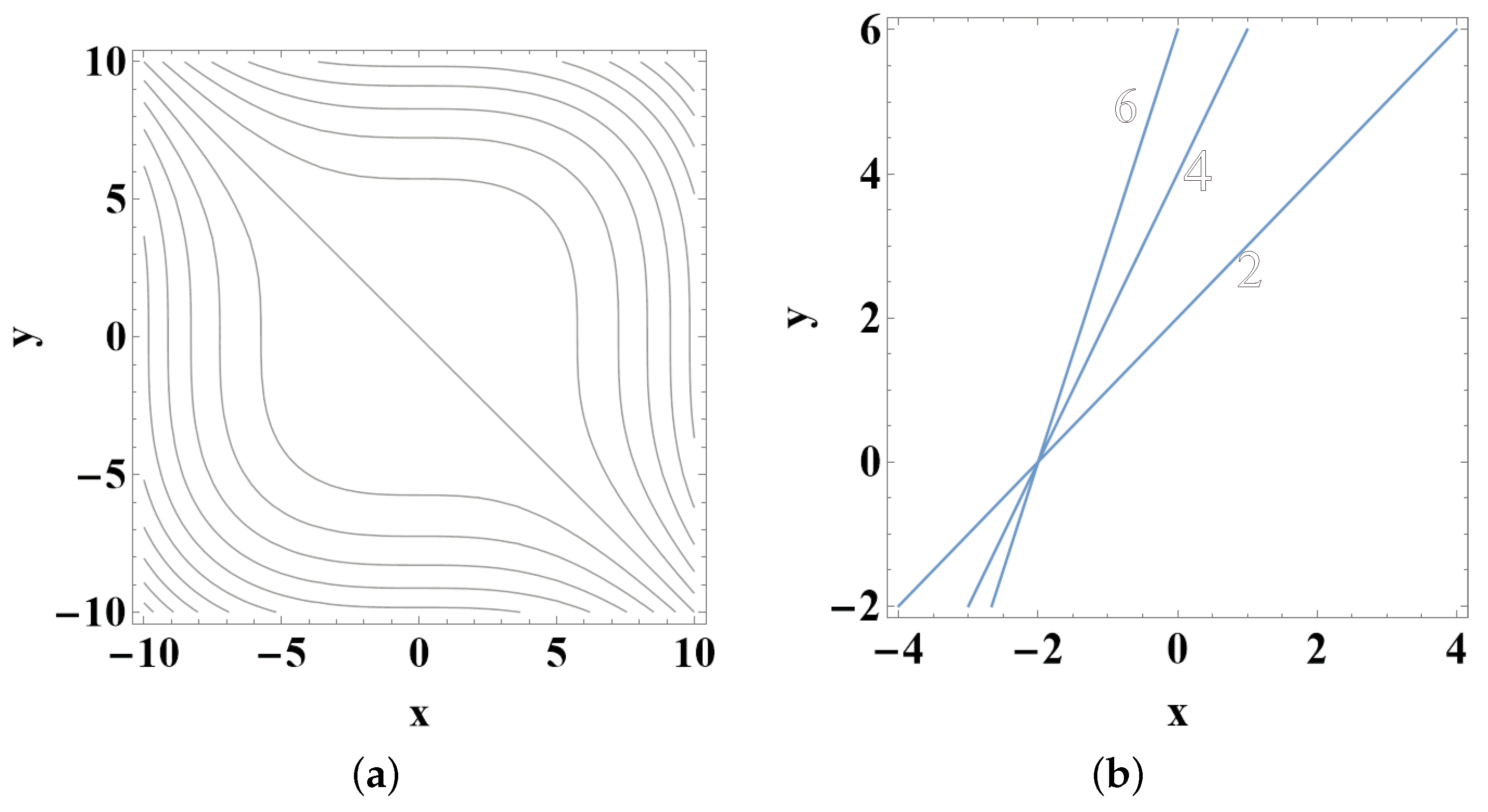
As a conclusion, the potential takes the form

$$V(x,y)=a_{00}+a_{03}(-b_0{x}^3+y^3).$$

(80)

A contour plot of the potential (80) for $a_{00}=0,a_{03}=1,b_0=-1$ is given at Figure 3a.

Figure 3. (a) A contour plot of the potential (80) for $a_{00}=0,a_{03}=1,b_0=-1$. (b) Some members of the family of straight lines (97) for $c=1,2,3$ and $a_1=b_1=$ 2.

The energy of the family of orbits (77) is found to be

$$\mathcal{E}=a_{00}+\frac{1}{4}{a}_{03}(-1+27b_0^2)c.$$

(81)

Example 6.

We consider the family of orbits

$$f(x,y)=x^3+b_0{x}^{2}y-3x{y}^2=c,b_0=const.\ne 0$$

(82)

and the potential of the form (76). We insert it into (4) and we obtain the expression

$$q_1{x}^7+q_2{x}^{6}y+q_3{x}^5{y}^2+q_4{x}^4{y}^3+q_5{x}^3{y}^4+q_6{x}^2{y}^5+q_{7}x{y}^6+q_8{y}^7=0,$$

(83)

where the coefficients $q_j,j=1,\dots ,8$ are given in “Appendix A”. The relation (83) must be identically zero. Thus, we have:

$$a_{30}=\mp \frac{i}{3}\sqrt{\frac{5}{6}}{a}_{21},a_{12}=0,a_{03}=\frac{a_{21}}{3},b_0=\pm i\sqrt{\frac{15}{2}}.$$

(84)

or,

$$a_{30}=\mp \frac{4i}{3\sqrt{3}}{a}_{21},a_{12}=0,a_{03}=\frac{a_{21}}{3},b_0=\pm 2i\sqrt{3}.$$

(85)

So, we have three cases:

• Case 1. $b_0=\pm i\sqrt{\frac{15}{2}}$. In addition to $a_{12}=0$, this choice leads to $a_{21}=a_{30}=a_{03}=$ 0, which gives the trivial solution.
• Case 2. $b_0=-2i\sqrt{3}$. This choice leads to $a_{12}=0,a_{21}=-\frac{3}{4}i\sqrt{3}{a}_{30}$. If we set $a_{30}=-4i\sqrt{3}$, then we obtain $a_{21}=-9$ and finally we determine the coefficient $a_{03}$. It is $a_{03}=-$3. As a conclusion, the potential takes the form

  $$V(x,y)=a_{00}-(4i\sqrt{3}{x}^3+9x^{2}y+3y^3),$$

  (86)
  which produces the monoparametric family of orbits

  $$f(x,y)=x^3-2i\sqrt{3}{x}^{2}y-3x{y}^2=c.$$

  (87)
• Case 3. $b_0=2i\sqrt{3}$. This choice leads to $a_{12}=0,a_{21}=\frac{3}{4}i\sqrt{3}{a}_{30}$. If we set $a_{30}=4i\sqrt{3}$, then we obtain $a_{21}=-9$ and we find the coefficient $a_{03}$ at last. It is $a_{03}=-$3. As a conclusion, the potential is

  $$V(x,y)=a_{00}+4i\sqrt{3}{x}^3-9x^{2}y-3y^3,$$

  (88)

  which produces the monoparametric family of orbits

  $$f(x,y)=x^3+2i\sqrt{3}{x}^{2}y-3x{y}^2=c.$$

  (89)

So, only complex polynomial potentials of the third degree are found as solutions to the last cases.

7. Families of Straight Lines

If $\Gamma$ = 0 ($\Gamma$ is defined in (3)), then we have to study a one-parameter family of straight lines (FSL) in a 2D space. As it was shown by [17], potentials that produce a one-parametric family of curves as straight lines on the $xy$-plane have to satisfy the following necessary and sufficient differential condition

$$\begin{array}{c}\hfill V_x{V}_y(V_{xx}-V_{yy})=V_{xy}(V_x^2-V_y^2).\end{array}$$

(90)

We examined the following potentials:

• I. $V=F\left(u\right)+G\left(v\right)$, where $u=x+y,v=x-y$.
• II. $V=F\left(u\right)+G\left(v\right)$, where $u=x+iy,v=x-iy$ and $i^2=-1$.
• III. $V=F\left(x\right)+G\left(y\right)$.

Inserting $V=F(x+y)+G(x-y)$ into (90), we obtain

$$F^{″}\left(u\right)=G^{″}\left(v\right)=a_0=const.$$

(91)

Thus, the general solution of (91) is

$$\begin{array}{ccc}\hfill F\left(u\right)& =& \frac{1}{2}{a}_0{u}^2+a_{1}u+a_2,a_1,a_2=const.\hfill \\ \hfill G\left(v\right)& =& \frac{1}{2}{a}_0{v}^2+b_{1}v+b_2,b_1,b_2=const.\hfill \end{array}$$

(92)

Then, the potential has the form

$$V=\frac{1}{2}{a}_0(u^2+v^2)+a_{1}u+b_{1}v+a_2+b_2,$$

(93)

or, equivalently,

$$V(x,y)=a_0(x^2+y^2)+a_1(x+y)+b_1(x-y)+a_2+b_2.$$

(94)

Then, we find the corresponding family of straight lines. This is ([17], p. 4)

$$\gamma =-\frac{V_x}{V_y}.$$

(95)

For the first case (94), we obtain

$$\gamma =-\frac{2a_{0}x+a_1+b_1}{2a_{0}y+a_1-b_1}.$$

(96)

Then, we solve Equation (6) and we find the family of straight lines

$$f(x,y)=\frac{2a_{0}y+a_1-b_1}{2a_{0}x+a_1+b_1}=c.$$

(97)

Some members of the family of straght lines (97) are presented at Figure 3b.

Inserting $V=F(x+iy)+G(x-iy)$ into (90), we obtain

$$-{\left[G^{\prime }\left(v\right)\right]}^2{F}^{″}\left(u\right)+{\left[F^{\prime }\left(u\right)\right]}^2{G}^{″}\left(v\right)=0,u=x+iy,v=x-iy,$$

(98)

or, equivalently,

$$\frac{F^{″}\left(u\right)}{{\left[F^{\prime }\left(u\right)\right]}^2}=\frac{G^{″}\left(v\right)}{{\left[G^{\prime }\left(v\right)\right]}^2}=a_0=const.\ne 0.$$

(99)

We set $F^{\prime }\left(u\right)=H\left(u\right)$, and by using (99), we obtain

$$H^{\prime }\left(u\right)=a_{0}H{\left(u\right)}^2,$$

(100)

with the general solution

$$H\left(u\right)=-\frac{1}{a_{0}u+a_1},a_1=const.$$

(101)

Thus, the function $F=F\left(u\right)$ is found to be

$$F\left(u\right)=\int H\left(u\right)du=-\frac{1}{a_0}log(a_{0}u+a_1)+a_2,a_2=const.$$

(102)

Working in a similar way with the right hand of Equation (99), we find that

$$G\left(v\right)=-\frac{1}{a_0}log(a_{0}v+b_1)+b_2,b_2=const.$$

(103)

The potential $V=V(x,y)$ takes a more concise form

$$V(x,y)=-\frac{1}{a_0}log\left[a_0(x+iy)+a_1)(a_0(x-iy)+b_1)\right]+a_2+b_2.$$

(104)

or, equivalently,

$$V(x,y)=-\frac{1}{a_0}log\left[(a_0^2(x^2+y^2)+(a_0{b}_1+a_0{a}_1)x+i(a_0{b}_1-a_1{a}_0)y+a_1{b}_1\right]+a_2+b_2.$$

(105)

Then, the family of straight lines is determined by

$$\gamma =-\frac{2a_0^{2}x+(a_0{b}_1+a_0{a}_1)}{2a_0^{2}y+i(a_0{b}_1-a_1{a}_0)}$$

(106)

and the family of straight lines is

$$f(x,y)=\frac{2a_0^{2}y+i(a_0{b}_1-a_1{a}_0)}{2a_0^{2}x+(a_0{b}_1+a_0{a}_1)}=c.$$

(107)

Finally, we insert $V=F\left(x\right)+G\left(y\right)$ into (90) and obtain

$$F^{″}\left(x\right)=G^{″}\left(y\right)=a_0=const.$$

(108)

Thus, the general solution of (108) is

$$\begin{array}{ccc}\hfill F\left(x\right)& =& \frac{1}{2}{a}_0{x}^2+a_{1}x+a_2,a_1,a_2=const.,\hfill \\ \hfill G\left(y\right)& =& \frac{1}{2}{a}_0{y}^2+b_{1}y+b_2,b_1,b_2=const.\hfill \end{array}$$

(109)

Then, the potential has the form

$$V=\frac{1}{2}{a}_0(x^2+y^2)+a_{1}x+b_{1}y+a_2+b_2,$$

(110)

Then, the family of straight lines is determined by

$$\gamma =-\frac{a_{0}x+a_1}{a_{0}y+b_1}$$

(111)

and the family of straight lines is

$$f(x,y)=\frac{a_{0}y+b_1}{a_{0}x+a_1}=c.$$

(112)

8. Conclusions

In the present paper, we studied four solvable versions of the two-dimensional inverse problem of dynamics. We studied monoparametric families of regular orbits $f(x,y)=c$ = const., which are compatible with two-dimensional potentials $V=V(x,y)$.

We dealt with the basic PDE of the inverse problem of dynamics, i.e., Equation (4), taking into account that the quantity $\Gamma$ is not zero (Section 2). We studied potentials of a special form, which have some properties that are related with physical problems. We focused our interest on potentials that satisfy the 2D wave equation, the well-known Laplace equation and separable potentials that have many applications in physical problems. In order to obtain interesting results, we studied known curves that lie on the $xy$-plane, e.g., circles, ellipses, parabolas, etc., which can be traced by a test particle of the unit mass as orbits. Our results were not restricted only to real potentials, but we extended them to complex potentials, which can give rise to a preassigned family of orbits. Our aim was to find a suitable pair of orbits compatible with these potentials. All the results are really new and original. Our study has been extended to the three-dimensional inverse problem of Newtonian dynamics. In a recent paper [21], we studied two-parametric families of orbits produced by central or polynomial potentials and we gave an application to the 3D harmonic oscillator. Furthermore, we studied families of orbits produced by homogeneous potentials on the outside of a material concentration [22]. In this case, the potentials have to satisfy the 3D Laplace equation too, i.e., ${\nabla }^{2}V$ = 0.

The present paper offers a new idea to the reader about how we treat potentials of a special form and combine them with the 2D inverse problem of dynamics by using the basic equations. The one-dimensional potentials consist of a special case of potentials and were examined separately. The families of the planar orbits compatible with them were also found and are presented in Table 1. Finally, we studied the case of straight lines, which is a special category of orbits in a 2D space.

References

- Szebehely, V. On the determination of the potential by satellite observations. Convegno Internazionale Sulla Rotazione Della Terra Oss. Satelliti Artif. 1974, 44, 31–35. [Google Scholar]
- Bozis, G. Generalization of Szebehely’s Equation. Celest. Mech. 1983, 29, 329–334. [Google Scholar] [CrossRef]
- Puel, F. Intrinsic formulation of the equation of Szebehely. Celest. Mech. 1984, 32, 209–216. [Google Scholar] [CrossRef]
- Bozis, G.; Tsarouhas, G. Conservative fields derived from two monoparametric families of planar orbits. Astron. Astrophys. 1985, 145, 215–220. [Google Scholar]
- Bozis, G. Szebehely’s inverse problem for finite symmetrical material concentrations. Astron. Astrophys. 1984, 134, 360–364. [Google Scholar]
- Bozis, G.; Grigoriadou, S. Families of planar orbits generated by homogeneous potentials. Celest. Mech. Dyn. Astr. 1993, 57, 461–472. [Google Scholar] [CrossRef]
- Bozis, G.; Anisiu, M.-C.; Blaga, C. Inhomogeneous potentials producing homogeneous orbits. Astron. Nach. 1997, 318, 313–318. [Google Scholar] [CrossRef]
- Bozis, G.; Stefiades, A. Geometrically similar orbits in homogeneous potentials. Inverse Probl. 1993, 9, 233–240. [Google Scholar] [CrossRef]
- Bozis, G.; Ichtiaroglou, S. Boundary Curves for Families of Planar Orbits. Celest. Mech. Dyn. Astr. 1993, 58, 371–385. [Google Scholar] [CrossRef]
- Bozis, G. The inverse problem of dynamics: Basic facts. Inverse Probl. 1995, 11, 687–708. [Google Scholar] [CrossRef]
- Anisiu, M.-C. An alternative point of view on the equations of the inverse problem of dynamics. Inverse Probl. 2004, 20, 1865–1872. [Google Scholar] [CrossRef]
- Bozis, G.; Anisiu, M.-C. A solvable version of the inverse problem of dynamics. Inverse Probl. 2005, 21, 487–497. [Google Scholar] [CrossRef]
- Grigoriadou, S.; Bozis, G.; Elmabsout, B. Solvable cases of Szebehely’s equation. Celest. Mech. Dyn. Astr. 1999, 74, 211–221. [Google Scholar] [CrossRef]
- Anisiu, M.-C.; Bozis, G.; Blaga, C. Special families of orbits in the direct problem of dynamics. Celest. Mech. Dyn. Astr. 2004, 88, 245–257. [Google Scholar] [CrossRef]
- Blaga, C.; Anisiu, M.-C.; Bozis, G. New solutions in the direct problem of dynamics. PADEU 2006, 17, 13. [Google Scholar]
- Bozis, G.; Anisiu, M.-C.; Blaga, C. A solavable version of the direct problem of dynamics. Rom. Astron. J. 2000, 10, 59–70. [Google Scholar]
- Bozis, G.; Anisiu, M.-C. Families of straight lines in planar potentials. Rom. Astron. J. 2001, 11, 27–43. [Google Scholar]
- Kotoulas, T. Monoparametric families of orbits produced by planar potentials. Axioms 2023, 12, 423. [Google Scholar] [CrossRef]
- Ichtiaroglou, S.; Meletlidou, E. On monoparametric families of orbits sufficient for integrability of planar potentials with linear or quadratic invariants. J. Phys. A. Math. Gen. 1990, 23, 3673–3679. [Google Scholar] [CrossRef]
- Ramani, A.; Dorizzi, B.; Grammaticos, B. Painlevé conjecture revisited. Phys. Rev. Let. 1982, 49, 1539–1541. [Google Scholar] [CrossRef]
- Kotoulas, T. Families of orbits produced by three-dimensional central and polynomial potentials: An application to the 3D harmonic oscillator. Axioms 2023, 12, 461. [Google Scholar] [CrossRef]
- Kotoulas, T. 3D homogeneous potentials generating two-parametric families of orbits on the outside of a material concentration. Eur. Phys. J. Plus 2023, 138, 124. [Google Scholar] [CrossRef]
Disclaimer/Publisher’s Note: The statements, opinions and data contained in all publications are solely those of the individual author(s) and contributor(s) and not of MDPI and/or the editor(s). MDPI and/or the editor(s) disclaim responsibility for any injury to people or property resulting from any ideas, methods, instructions or products referred to in the content. |
© 2024 by the author. Licensee MDPI, Basel, Switzerland. This article is an open access article distributed under the terms and conditions of the Creative Commons Attribution (CC BY) license (https://creativecommons.org/licenses/by/4.0/).