Portmanteau Test for ARCH-Type Models by Using High-Frequency Data

Abstract

The portmanteau test is an effective tool for testing the goodness of fit of models. Motivated by the fact that high-frequency data can improve the estimation accuracy of models, a modified portmanteau test using high-frequency data is proposed for ARCH-type models in this paper. Simulation results show that the empirical size and power of the modified test statistics of the model using high-frequency data are better than those of the daily model. Three stock indices (CSI 300, SSE 50, CSI 500) are taken as an example to illustrate the practical application of the test.

1. Introduction

Securities trading has always been a prominent topic in the financial sector, and volatility serves as a crucial indicator for analyzing fluctuations in trading price data. Volatility reflects the expected level of price instability in a financial asset or market, which greatly influences investment decisions [1]. In the field of volatility modeling, the autoregressive conditional heteroscedasticity (ARCH) model and the generalized autoregressive conditional heteroscedasticity (GARCH) model are widely recognized as two fundamental models [2]. Let $y_t$ be the log-return of day t. The ARCH model proposed by Engle (1982) [3] is structured as follows:

$$y_t={\sigma }_t{\epsilon }_t,$$

$${\sigma }_t^2=\omega +{\alpha }_1{y}_{t-1}^2+{\alpha }_2{y}_{t-2}^2+\dots +{\alpha }_q{y}_{t-q}^2,$$

where ${\epsilon }_t$ is an independent and identically distributed (i.i.d.) sequence, and ${\sigma }_t$ represents the volatility of $y_t$. Additionally, it is assumed that the expectation of ${\epsilon }_t$ is zero, i.e., $E\left[{\epsilon }_t\right]=0$, and the expectation of ${\epsilon }_t^2$ is equal to one, i.e., $E\left[{\epsilon }_t^2\right]=1$. The parameters $(\omega ,{\alpha }_1,{\alpha }_2,\dots ,{\alpha }_q)$ are the coefficients associated with the lagged squared observations $(1,y_{t-1}^2,y_{t-2}^2,\dots ,y_{t-q}^2)$, which need to be estimated. ARCH models are commonly employed in time-series modeling and analysis. However, when the order q of the ARCH(q) model is large, the number of parameters that require estimation increases. This can lead to challenges in estimation, particularly in cases with finite samples where estimation efficiency may decrease. Furthermore, it is possible for the estimated parameter values to turn out negative. To address these limitations, Bollerslev (1986) [4] proposed the generalized autoregressive conditional heteroscedasticity (GARCH) model. For the pure GARCH(1,1) model, the conditional variance equation is expressed as follows:

$${\sigma }_t^2=\omega +\alpha y_{t-1}^2+\beta {\sigma }_{t-1}^2.$$

(1)

Obviously, Formula (1) is an iterative equation. Let $t=t-1$. Then

$${\sigma }_{t-1}^2=\omega +\alpha y_{t-2}^2+\beta {\sigma }_{t-2}^2.$$

(2)

From (1) and (2), we obtain

$$\begin{array}{cc}\hfill {\sigma }_t^2& =\omega +\alpha y_{t-1}^2+\beta (\omega +\alpha y_{t-2}^2+\beta {\sigma }_{t-2}^2)\hfill \\ & =(1+\beta )\omega +\alpha y_{t-1}^2+\alpha \beta y_{t-2}^2+{\beta }^2{\sigma }_{t-2}^2.\hfill \end{array}$$

Repeating the process above, we expand ${\sigma }_{t-2}^2,{\sigma }_{t-3}^2,\dots$. Then, we can obtain an infinite-order ARCH model. Since the GARCH model is a generalization of the ARCH model, they are collectively referred to as the ARCH-type models. In financial data analysis, apart from heteroscedasticity, there are other prominent characteristics, such as the leverage effect (Black, 1976) [5]. To address this, Geweke (1986) [6] introduced the asymmetric log-GARCH model, while Engle et al. (1993) [7] introduced the asymmetric power GARCH model to account for the leverage effect. Furthermore, Drost and Klassen (1997) [8] modified the pure GARCH(1,1) model as follows:

$$y_t=v_t\tau {\epsilon }_t,$$

(3)

$$v_t^2=1+\gamma y_{t-1}^2+\beta v_{t-1}^2.$$

(4)

For the ARCH(q) case, the conditional variance equation is given by

$$v_t^2=1+{\gamma }_1{y}_{t-1}^2+{\gamma }_2{y}_{t-2}^2+\dots +{\gamma }_q{y}_{t-q}^2.$$

(5)

When $v_t\tau ={\sigma }_t$, ${\tau }^2=\omega$, and $\gamma {\tau }^2=\alpha$, the models (3) and (4) can be transformed into the pure GARCH(1,1) model. Similarly, the models (3) and (5) can be transformed into the pure ARCH(q) model. The advantage of this model is that the standardization of ${\epsilon }_t$ only affects the parameter $\tau$. By standardizing the residuals, they are made unit variance, simplifying the estimation process and allowing the focus to be on estimating the parameters of interest without being influenced by the scale of the residuals.

With the advancement of information technology, obtaining intraday high-frequency data has become effortless, and such data often contain valuable information. Recognizing this, Visser (2011) [9] introduced high-frequency data into models (3) and (4), leading to improved efficiency in model parameters estimation. Subsequently, numerous researchers have extensively explored the enhancement of classical models by utilizing high-frequency data. Huang et al. (2015) [10] incorporated high-frequency data into the GJR model (named by the proponents Glosten, Jagannathan and Runkel) [11] and examined a range of robust M-estimators [12]. Wang et al. (2017) [13] employed composite quantile regression to examine the GARCH model using high-frequency data. Other notable studies include Fan et al. (2017) [14], Deng et al. (2020) [15], and Liang et al. (2021) [16].

In addition to model parameter estimation, model testing plays a crucial role in time-series modeling and analysis as researchers seek to assess the adequacy of the established models. Portmanteau tests have been widely used for this purpose. The earliest work in this area can be traced back to Box and Pierce (1970) [17], who demonstrated the utility of square-residual autocorrelations for model testing. Since then, several researchers have applied this test to time-series models, including Granger et al. (1978) [18] and Mcleod and Li (1983) [19]. For instance, Engle and Bollerslev (1986) [20] and Pantula (1988) [21] proposed the test to examine the presence of ARCH in the error term. However, Li and Mak (1994) [22] showed that the variance of the residual autocorrelation function is not idempotent when using ARCH-type models. To overcome this issue, they developed a modified statistic that incorporated the variance of the residual autocorrelation function. They also proved that when the parameter estimates follow asymptotic normality, the test statistic follows a chi-square distribution. After the emergence of the quasi-maximum exponential likelihood estimation (QMELE) method [23], Li and Li (2005) [24] generalized the test statistic proposed by Li and Mak [22] using a new estimation method. They also proposed a similar test statistic for the autocorrelation function with absolute residuals $|{\epsilon }_t|$. Carbon and Francq (2011) [25] extended the test of Li and Mak [22] to the asymmetric power GARCH model. Furthermore, Chen and Zhu (2015) [26] constructed a rank-based portmanteau test based on Li and Mak’s [22] statistic. They modified the autocorrelation function of the residuals ${\epsilon }_t$ to the autocorrelation function of the rank-based residuals $sgn({\epsilon }_t^2-1)$, making the new test applicable to heavy-tailed data. Even today, scholars like Li and Zhang (2022) [27] continue to show great interest in studying the extension of these tests.

Motivated by the works of Li and Mak (1994) [22] and Visser (2011) [9], this paper introduces a modified portmanteau test for diagnosing ARCH-type models using high-frequency data. The paper also discusses the general procedure for constructing portmanteau test statistics for ARCH-type models based on high-frequency data. It is demonstrated that under weaker conditions such as having a finite residual fourth-order moment and other regularity conditions, the proposed portmanteau test follows a chi-square distribution.

This paper is structured as follows. Section 2 discusses the estimation for ARCH-type models. Section 3 covers the construction of the portmanteau test statistics and provides the corresponding asymptotic distribution. Section 4 presents the simulation process and the related results. Section 5 includes three real data examples along with the analysis of the corresponding results. Finally, the assumptions, proofs, and additional results are deferred to the Appendix B.

2. Estimation Using High-Frequency Data

To introduce high-frequency data, the structure of the log-returns equation has been enhanced. The observed intraday log-return process $Y_t\left(u\right)$ for day t is associated with the standardized intraday trading time variable u, which ranges from 0 to 1. According to Visser (2011) [9], the modified model is a scaling GARCH(1,1) model, which is expressed as:

$$Y_t\left(u\right)=v_t\tau {\epsilon }_t\left(u\right),0\le u\le 1,$$

(6)

$$v_t^2=1+\gamma y_{t-1}^2+\beta v_{t-1}^2,$$

(7)

where $\left\{{\epsilon }_t\left(u\right)\right\}$ represents a standardized process. The assumption is made that for any $k\ne l$, ${\epsilon }_k(·)$ and ${\epsilon }_l(·)$ are independent of each other and share the same distribution. When u is set to 1, the following relationships hold:

$$Y_t\left(1\right)=y_t,{\epsilon }_t\left(1\right)={\epsilon }_t,E{\epsilon }_t{\left(1\right)}^2=1.$$

Hence, when u is set to 1, models (6) and (7) are transformed into models (3) and (4), which combine the scaling model with the pure GARCH model.

In order to estimate the parameters, the scaling model utilizes a volatility proxy. This proxy reduces high-dimensional information to a single dimension. Furthermore, when the conditional mean is zero, the volatility proxy serves as an unbiased estimate of the conditional variance. Specifically, the volatility proxy $H(·)$ is a statistic derived from intraday data and satisfies the following property of positive homogeneity:

$$H\left(\rho Y_t\left(u\right)\right)=\rho H\left(Y_t\left(u\right)\right)>0,\rho \le 0.$$

When t is fixed, $v_t$ becomes a constant. By applying the homogeneity property of $H(·)$, it can be observed that

$$H\left(Y_t\left(u\right)\right)=H\left(v_t\tau {\epsilon }_t\left(u\right)\right)=v_t\tau H\left({\epsilon }_t\left(u\right)\right).$$

For convenience, let $H_t\triangleq H\left(Y_t\left(u\right)\right)$, ${\mu }_H\triangleq \sqrt{E\left(H^2\left({\epsilon }_t\left(u\right)\right)\right)}$, ${\tau }_H\triangleq {\mu }_H\tau$, and ${\epsilon }_t^{*}\triangleq H\left({\epsilon }_t\left(u\right)\right)/{\mu }_H$. Then, the volatility proxy GARCH model has the following structure:

$$H_t=v_t{\tau }_H{\epsilon }_t^{*},$$

(8)

$$v_t^2=1+\gamma y_{t-1}^2+\beta v_{t-1}^2,$$

(9)

where $\left\{{\epsilon }_t^{*}\right\}$ is also an i.i.d. sequence that satisfies $E{\epsilon }_t^{*2}=1$. ${({\tau }_H,\gamma ,\beta )}^{\prime }$ is the parameter of the models (8) and (9) that needs to be estimated. For simplicity, models (8) and (9) are referred to as the VP-GARCH(1,1) model.

In the case of ARCH(q), the return equation aligns with Formula (8), while the conditional variance equation is expressed as:

$$v_t^2=1+{\gamma }_1{y}_{t-1}^2+{\gamma }_2{y}_{t-2}^2+\dots +{\gamma }_q{y}_{t-q}^2.$$

(10)

Similarly, the parameter vector ${({\tau }_H,{\gamma }_1,{\gamma }_2,\dots ,{\gamma }_q)}^{\prime }$ represents the parameters of models (8) and (10), which require estimation. The models (8) and (10) are referred to as the VP-ARCH(q) model.

The Gaussian quasi-maximum likelihood estimation (QMLE) [9] is employed to estimate the parameters of models (8) and (9) and models (8) and (10). The QMLE of $\mathit{\theta }$ is defined as:

$$\tilde{\mathit{\theta }}=arg\underset{\mathit{\theta }\in \mathbf{\Theta }}{min}{L}_n\left(\mathit{\theta }\right),L_n\left(\mathit{\theta }\right)=\frac{1}{2}\sum _{t=1}^n\left(log\left(v_t^2{\tau }_H^2\right)+\frac{H_t^2}{v_t^2{\tau }_H^2}\right).$$

(11)

To differentiate between them, the parameter vector estimate using low-frequency data is denoted as $\widehat{\mathit{\theta }}$, while the parameter vector estimate using high-frequency data is denoted as $\tilde{\mathit{\theta }}$. The asymptotic normality of the parameter estimates for models (8) and (9) has been proven by Visser [9]. This conclusion can also be applied to models (8) and (10). Therefore, the following asymptotic normality can be obtained:

$$\sqrt{n}(\tilde{\mathit{\theta }}-{\mathit{\theta }}_0)\stackrel{d}{⟶}N(0,var\left({\epsilon }_t^{*2}\right){\mathit{G}}^{-1}),$$

$$\mathit{G}=E\left(\frac{1}{{\sigma }_{H,t}^4}\frac{\partial {\sigma }_{H,t}^2}{\partial \mathit{\theta }}\frac{\partial {\sigma }_{H,t}^2}{\partial {\mathit{\theta }}^{\prime }}\right),{\sigma }_{H,t}=v_t{\tau }_H.$$

In particular, when ${\tau }_H$ is known, let $\mathit{\eta }={(\gamma ,\beta )}^{\prime }$ be the parameter vector for models (8) and (9), and let $\mathit{\eta }={({\gamma }_1,\dots ,{\gamma }_q)}^{\prime }$ denote the parameter vector for models (8) and (10). Then

$$\mathit{G}=\mathrm{cov}\left(\frac{1}{v_t^2}\frac{\partial v_t^2}{\partial \mathit{\eta }},\frac{1}{v_t^2}\frac{\partial v_t^2}{\partial {\mathit{\eta }}^{\prime }}\right).$$

3. Portmanteau Test

3.1. Traditional Portmanteau Test

The portmanteau test is employed to evaluate the adequacy of the model’s fit. This statistical test is constructed based on the squared residual autocorrelation function. In cases where the volatility model is inadequate, a certain level of correlation between the squared residual terms exists.

In this paper, the null hypothesis is that the squared residual autocorrelation functions are irrelevant, indicating that the hypothesized model is adequate. The sample squared residual autocorrelation function ${\widehat{r}}_k$ is calculated as follows:

$${\widehat{r}}_k=\frac{{\sum }_{t=k+1}^n(y_t^2/{\widehat{\sigma }}_t^2-1)(y_{t-k}^2/{\widehat{\sigma }}_{t-k}^2-1)}{{\sum }_{t=1}^n{(y_t^2/{\widehat{\sigma }}_t^2-1)}^2},k=1,2,3,\dots$$

According to the central limit theorem, it can be proven that ${\widehat{r}}_k$ follows an asymptotic normal distribution under the null hypothesis. To obtain the test statistic, a finite vector of autocorrelation functions ${\widehat{\mathit{r}}}_M={({\widehat{r}}_1,{\widehat{r}}_2,\dots ,{\widehat{r}}_m)}^{\prime }$ is considered, where m is the maximum lag order of ${\widehat{r}}_k$. Let $\mathit{D}$ denote the asymptotic variance of ${\mathit{r}}_M$. The portmanteau test statistic $Q^2$ can be formulated as:

$$Q^2=n{\widehat{\mathit{r}}}_M^{\prime }{\widehat{\mathit{D}}}^{-1}{\widehat{\mathit{r}}}_M.$$

(12)

Under Assumptions 3 and 4, $\frac{1}{n}{\sum }_{t=1}^n{(y_t^2/{\widehat{\sigma }}_t^2-1)}^2$ converges to constant $E{({\epsilon }_t^2-1)}^2$ in probability. Here, $E{({\epsilon }_t^2-1)}^2$ can be estimated by ${\widehat{C}}_0$, where

$${\widehat{C}}_0=\frac{1}{n}\sum _{t=1}^n\frac{y_t^4}{{\widehat{\sigma }}_t^4}-1.$$

Therefore, only the asymptotic distribution of ${\widehat{C}}_k$ needs to be considered, where

$${\widehat{C}}_k=\sum _{t=k+1}^n(\frac{y_t^2}{{\widehat{\sigma }}_t^2}-1)(\frac{y_{t-k}^2}{{\widehat{\sigma }}_{t-k}^2}-1),k=1,2,\dots ,m.$$

(13)

So, Formula (12) can be changed into

$$Q^2=n{\widehat{\mathit{C}}}_M^{\prime }{\widehat{\mathit{V}}}^{-1}{\widehat{\mathit{C}}}_M\stackrel{d}{⟶}{\chi }^2\left(m\right),$$

where ${\widehat{\mathit{C}}}_M={({\widehat{C}}_1,{\widehat{C}}_2,\dots ,{\widehat{C}}_m)}^{\prime }$, and V is the asymptotic variance of ${\mathit{C}}_M$.

The statistic $Q^2$ asymptotically follows a chi-square distribution with m degrees of freedom. By setting the significance level at 0.05, if the calculated result exceeds the $95\%$ quantile ${\chi }_{0.95}^2\left(m\right)$, the null hypothesis will be rejected. Conversely, if the calculated result is below the quantile, the null hypothesis will not be rejected, indicating that the model can be considered adequate.

3.2. Portmanteau Test Using High-Frequency Data

From Equation (13), we can observe that the estimate ${\widehat{C}}_k$ is dependent on the estimate of ${\widehat{\sigma }}_t^2$. The estimator ${\widehat{\sigma }}_t^2$ is a function of $\mathit{\theta }$. Given that the estimator $\tilde{\mathit{\theta }}$ is obtained using high-frequency data, the volatility estimator ${\tilde{\sigma }}_t^2\left(\tilde{\mathit{\theta }}\right)$ can be easily obtained. Additionally, the statistic ${\tilde{C}}_k\left(\tilde{\mathit{\theta }}\right)$ can be calculated as follows:

$${\tilde{C}}_k\left(\tilde{\mathit{\theta }}\right)=\sum _{t=k+1}^n(\frac{y_t^2}{{\tilde{\sigma }}_t^2\left(\tilde{\mathit{\theta }}\right)}-1)(\frac{y_{t-k}^2}{{\tilde{\sigma }}_{t-k}^2\left(\tilde{\mathit{\theta }}\right)}-1),k=1,2,\dots .$$

(14)

Similarly,

$${\tilde{C}}_0=\frac{1}{n}\sum _{t=1}^n\frac{y_t^4}{{\tilde{\sigma }}_t^4}-1.$$

Furthermore, the asymptotic distribution of the estimator $\tilde{\mathit{\theta }}$ differs from that of the estimator $\widehat{\mathit{\theta }}$, which is a difference that further impacts the asymptotic variance of ${\tilde{C}}_k$. Let $\widetilde{{\mathit{V}}_1}$ denote the modified variance estimator. The following theorem can then be derived.

Theorem 1.

If Assumptions 1–5 are satisfied, then under the null,

$${\tilde{Q}}^2=n{\tilde{\mathit{C}}}_M^{\prime }{\tilde{\mathit{V}}}_1^{-1}{\tilde{\mathit{C}}}_M\stackrel{d}{⟶}{\chi }^2\left(m\right),$$

where ${\tilde{\mathit{C}}}_M={({\tilde{C}}_1,{\tilde{C}}_2,\dots ,{\tilde{C}}_m)}^{\prime }$, ${\tilde{\mathit{V}}}_1={\tilde{C}}_0^2{\mathit{I}}_M+{\tilde{C}}_H\tilde{\mathit{X}}{\tilde{\mathit{G}}}^{-1}{\tilde{\mathit{X}}}^{\prime }-2{\tilde{C}}_{H,0}\tilde{\mathit{X}}{\tilde{\mathit{G}}}^{-1}{\tilde{\mathit{X}}}_H^{\prime }$,

$$\begin{array}{cc}\hfill {\tilde{C}}_H& =\frac{1}{n}\sum _{t=1}^n\frac{H_t^4}{{\tilde{\sigma }}_{H,t}^4}-1,{\tilde{C}}_{H,0}=\frac{1}{n}\sum _{t=1}^n\left\{(\frac{H_t^2}{{\tilde{\sigma }}_{H,t}^2}-1)(\frac{y_t^2}{{\tilde{\sigma }}_t^2}-1)\right\},\hfill \\ \hfill \tilde{\mathit{X}}& ={({\tilde{X}}_1,{\tilde{X}}_2,\dots ,{\tilde{X}}_m)}^{\prime },{\tilde{\mathit{X}}}_H={({\tilde{X}}_{H,1},{\tilde{X}}_{H,2},\dots ,{\tilde{X}}_{H,m})}^{\prime },\hfill \\ \hfill {\tilde{X}}_k& =-\frac{1}{n}\sum _{t=k+1}^n\left(\frac{1}{{\tilde{\sigma }}_t^2}\frac{\partial {\sigma }_t^2}{\partial \theta }\right)(\frac{y_{t-k}^2}{{\tilde{\sigma }}_{t-k}^2}-1),k=1,2,\dots ,m,\hfill \\ \hfill {\tilde{X}}_{H,k}& =-\frac{1}{n}\sum _{t=1}^n\left(\frac{1}{{\tilde{\sigma }}_{H,t}^2}\frac{\partial {\sigma }_{H,t}^2}{\partial \theta }\right)(\frac{y_{t-k}^2}{{\tilde{\sigma }}_{t-k}^2}-1),k=1,2,\dots ,m.\hfill \end{array}$$

The proof of Theorem 1 is presented in Appendix A.2.

Indeed, the presence of the parameter ${\tau }_H$ poses challenges in obtaining the QMLE $\tilde{\mathit{\theta }}$ in practical applications. However, these challenges can be overcome if an appropriate volatility proxy $H(·)$ is identified. When the volatility proxy $H(·)$ satisfies $E{H}^2\left({\epsilon }_t\left(u\right)\right)=1$, indicating ${\mu }_H=1$, then $\tau ={\tau }_H$. Assuming ${\mu }_H=1$, we can establish the following lemma.

Lemma 1.

If Assumptions 1–6 are satisfied, then under the null,

$${\tilde{Q}}^2=n{\tilde{\mathit{C}}}_M^{\prime }{\widetilde{{\mathit{V}}_2}}^{-1}{\tilde{\mathit{C}}}_M\stackrel{d}{⟶}{\chi }^2\left(m\right),$$

where $\widetilde{{\mathit{V}}_2}={\tilde{C}}_0^2{\mathit{I}}_M+({\tilde{C}}_H-2{\tilde{C}}_{H,0})\tilde{\mathit{X}}{\tilde{\mathit{G}}}^{-1}{\tilde{\mathit{X}}}^{\prime }$.

The proof of Lemma 1 is also provided in Appendix A.2.

4. Simulation

In this section, the finite-sample performance of the proposed method is examined through Monte Carlo simulations [28]. All data generation, results calculation, and figures plotting in this section are accomplished by running the R program.

In practical applications, the log-return series $Y_t\left(u\right)$ can be calculated based on the stock price. However, in the simulation, prior to simulating the generation of $Y_t\left(u\right)$, it is necessary to generate the high-frequency residual sequences. Following Visser [9], the high-frequency residual sequences ${\epsilon }_t\left(u\right)$ can be generated using the stationary Ornstein–Uhlenbeck process [29]:

$$d{\mathsf{\Gamma }}_t\left(u\right)=-\delta ({\mathsf{\Gamma }}_t\left(u\right)-{\mu }_{\mathsf{\Gamma }})du+{\sigma }_{\mathsf{\Gamma }}d{B}_t^{\left(2\right)}\left(u\right),$$

$$d{\epsilon }_t\left(u\right)=exp\left({\mathsf{\Gamma }}_t\left(u\right)\right)d{B}_t^{\left(1\right)}\left(u\right),u\in [0,1],$$

where $d{B}_t^{\left(1\right)}$ and $d{B}_t^{\left(2\right)}$ are unrelated Brownian motions [30]. The initial value of ${\epsilon }_t\left(0\right)$ is set to 0, and ${\mathsf{\Gamma }}_t\left(0\right)$ is generated from a stable distribution $N({\mu }_{\mathsf{\Gamma }},{\sigma }_{\mathsf{\Gamma }}^2/2\delta )$. To simulate the Chinese stock exchange market, the interval [0, 1] is divided into 240 small equal intervals, representing every minute of intraday trading. The values of ${\mu }_{\mathsf{\Gamma }}$, ${\sigma }_{\mathsf{\Gamma }}$, and $\delta$ are set to

$$\delta =\frac{1}{2},{\sigma }_{\mathsf{\Gamma }}=\frac{1}{4},{\mu }_{\mathsf{\Gamma }}=-\frac{1}{16}.$$

This ensures that the expected value of ${\epsilon }_t^2\left(1\right)$ is equal to 1 [9]. The calculation of $Y_t\left(u\right)$ is based on the given parameter vector $\mathit{\theta }$ using Equations (6), (7) and (10). For ARCH(2), set $\eta ={(0.6,0.3)}^{\prime }$ and $\eta ={(0.4,0.25)}^{\prime }$. For VP-GARCH(1,1), set $\eta ={(0.1,0.6)}^{\prime }$ and $\eta ={(0.25,0.5)}^{\prime }$. The corresponding equation is as follows:

$$v_t^2=1+0.6y_{t-1}^2+0.3y_{t-2}^2,$$

(15)

$$v_t^2=1+0.4y_{t-1}^2+0.25y_{t-2}^2,$$

(16)

$$v_t^2=1+0.1y_{t-1}^2+0.6v_{t-1}^2,$$

(17)

$$v_t^2=1+0.25y_{t-1}^2+0.5v_{t-1}^2.$$

(18)

Eventually, volatility proxy is selected as the realized volatility (RV). Three sampling frequencies are considered: 5 min, 15 min, and 30 min, which are denoted as RV5, RV15, and RV30, respectively. Taking RV15 as an example, the formula is

$$Ht=RV{15}_t={\left(\sum _{t=1}^{16}[Y_t\left(u_{15i}\right)-Y_t\left(u_{15(i-1)}\right)]\right)}^{1/2}.$$

Similarly, for the high-frequency residual ${\epsilon }_t\left(u\right)$, the formula is

$$H\left({\epsilon }_t\left(u\right)\right)={\left(\sum _{t=1}^{16}[{\epsilon }_t\left(u_{15i}\right)-{\epsilon }_t\left(u_{15(i-1)}\right)]\right)}^{1/2}.$$

To evaluate the performance of the models, let n denote the sample size and four sample sizes are considered: 200, 300, 400, and 500. For each model, 1000 independent replications are generated. Then, the root mean squared error (RMSE) of parameter estimates can be calculated. The formula is as follows:

$$RMSE\left(\widehat{\eta }\right)=\sqrt{\frac{1}{1000}\sum _{i=1}^{1000}{({\widehat{\eta }}_i-\eta )}^2},$$

where ${\widehat{\eta }}_i$ is the parameter estimate for the i-th time and $\eta$ is the true value of the parameter. The RMSE results are presented in

Table 1. RMSE of parameter estimates under four volatility proxy models.

		$\mathit{n}=200$		$\mathit{n}=300$		$\mathit{n}=400$		$\mathit{n}=500$
model (15)		${\gamma }_1$	${\gamma }_2$	${\gamma }_1$	${\gamma }_2$	${\gamma }_1$	${\gamma }_2$	${\gamma }_1$	${\gamma }_2$
	$|y_t|$	0.1755	0.1282	0.1418	0.1088	0.1280	0.0941	0.1097	0.0819
	RV30	0.0788	0.0585	0.0656	0.0489	0.0563	0.0408	0.0490	0.0370
	RV15	0.0663	0.0497	0.0551	0.0410	0.0471	0.0346	0.0414	0.0319
	RV5	0.0573	0.0410	0.0480	0.0355	0.0412	0.0346	0.0353	0.0268
model (16)	$|y_t|$	0.1439	0.1197	0.1184	0.0994	0.1064	0.0847	0.0919	0.0801
	RV30	0.0676	0.0568	0.555	0.0462	0.0465	0.0378	0.0424	0.0344
	RV15	0.0568	0.0469	0.0480	0.0386	0.0385	0.0325	0.0367	0.0293
	RV5	0.0486	0.0392	0.0416	0.0327	0.0330	0.0278	0.0316	0.0253
model (17)		${\gamma }_1$	${\beta }_1$	${\gamma }_1$	${\beta }_1$	${\gamma }_1$	${\beta }_1$	${\gamma }_1$	${\beta }_1$
	$|y_t|$	0.0773	0.0777	0.0651	0.0656	0.0552	0.0559	0.0485	0.0499
	RV30	0.0372	0.0367	0.0304	0.0306	0.0267	0.0257	0.0228	0.0221
	RV15	0.0306	0.0302	0.0259	0.0257	0.0226	0.0217	0.0193	0.0188
	RV5	0.0268	0.0263	0.0226	0.0219	0.0197	0.0191	0.0165	0.0157
model (18)	$|y_t|$	0.1240	0.0941	0.0935	0.0750	0.0856	0.0670	0.0730	0.0573
	RV30	0.0529	0.0411	0.0426	0.0342	0.0373	0.0300	0.0324	0.0254
	RV15	0.0447	0.0342	0.0354	0.0282	0.0313	0.0252	0.0268	0.0219
	RV5	0.0370	0.0287	0.0305	0.0243	0.0263	0.0210	0.0232	0.0187

.

The $|y_t|$ in Table 1 represents the daily model, where $H_t=\left|y_t\right|$ is calculated using daily closing prices. Table 1 clearly shows that the estimation results obtained from the intraday models, using high-frequency data, outperform those of the daily model.

Additionally, it is necessary to examine the distribution of the statistic and compare its performance with the daily model. Therefore,

Table 2. Empirical size of four volatility proxies under four models.

		$\mathit{n}=200$	$\mathit{n}=300$	$\mathit{n}=400$	$\mathit{n}=500$
model (15)	$|y_t|$	0.039	0.033	0.037	0.031
	RV30	0.070	0.064	0.059	0.058
	RV15	0.071	0.064	0.052	0.057
	RV5	0.075	0.059	0.056	0.059
model (16)	$|y_t|$	0.030	0.029	0.033	0.019
	RV30	0.075	0.047	0.052	0.044
	RV15	0.075	0.055	0.054	0.049
	RV5	0.075	0.054	0.057	0.050
model (17)	$|y_t|$	0.024	0.035	0.028	0.030
	RV30	0.068	0.062	0.046	0.047
	RV15	0.061	0.071	0.054	0.054
	RV5	0.064	0.070	0.048	0.058
model (18)	$|y_t|$	0.037	0.024	0.035	0.027
	RV30	0.066	0.059	0.060	0.047
	RV15	0.064	0.064	0.062	0.050
	RV5	0.072	0.062	0.060	0.052

presents the empirical size values for this purpose.

We set $m=6$ and calculate the empirical size by determining the proportions of rejections based on the 95th percentile of ${\chi }^2\left(6\right)$. The results are presented in Table 2. It is evident that as the sample size increases, the results of the intraday models are closer to 0.05 compared to those of the daily model. It suggests that introducing high-frequency data can enhance the accuracy of the model.

Regarding the power, we define the alternative hypotheses for ARCH(2) and GARCH(1,1) as follows:

$$H_1:v_t^2=1+{\gamma }_1{y}_{t-1}^2+{\gamma }_2{y}_{t-2}^2+{\gamma }_3{y}_{t-3}^2,$$

$$H_1:v_t^2=1+{\gamma }_1^{\prime }{y}_{t-1}^2+{\gamma }_2^{\prime }{y}_{t-2}^2+{\beta }_1{v}_{t-1}^2,$$

where ${\gamma }_1$ and ${\gamma }_2$ are obtained from models (15) and models (16), respectively, while ${\gamma }_1^{\prime }$ and ${\beta }_1$ are obtained from models (17) and models (18), respectively, which are all fixed values. Next, we introduce ${\gamma }_3$ and ${\gamma }_2^{\prime }$ as variables to examine the impact on the power.

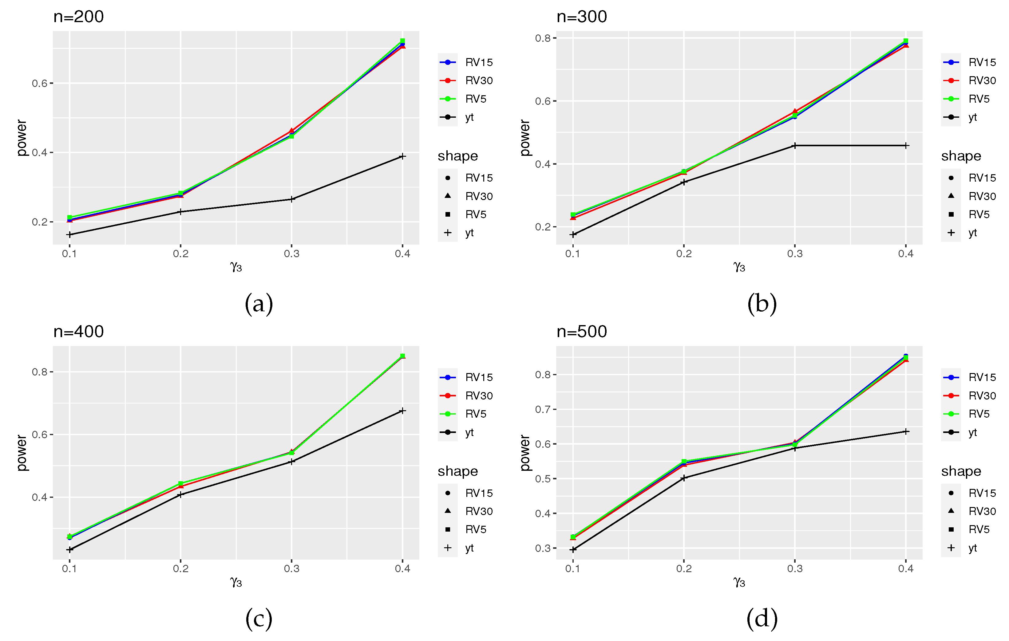
Figure 1 displays the power results of the ARCH(2) model, while Figure 2 presents the power results of the GARCH(1,1) model. The results for models (16) and (18) can be found in Appendix B (Figure A1 and Figure A2). From these figures, it is evident that the power curves of the intraday models exhibit clear distinctions from that of the daily model, although this effect diminishes as the sample size increases. Additionally, upon comparing the power of the four models, we observe that the ARCH model demonstrates a more pronounced power.

5. Application

In our analysis, we focus on three stock indices: the CSI 300, SSE 50, and CSI 500. The data cover the period from 2 January 2004 to 6 June 2019. After deleting missing data, we obtained a dataset consisting of 2610 consecutive days (8 April 2005 to 31 December 2015) for the CSI 300 index, 2856 consecutive days (2 January 2004 to 13 October 2015) for the SSE 50 index, and 2124 consecutive days (15 January 2007 to 13 October 2015) for the CSI 500 index. The calculations and figures presented in this section are generated using the R programming language.

To compute the high-frequency log-return $Y_t\left(u\right)$ [9], the following formula is employed:

$$Y_t\left(u\right)=[log{P}_t\left(u\right)-log{P}_{t-1}\left(u\right)]\times 100,u\in [0,1],$$

where $P_t\left(u\right)$ denotes the trading price within 240 min of day t, and $Y_t\left(1\right)=y_t$ denotes the closing price of day t. The log-return $Y_t\left(1\right)$ values for the three indices are depicted in Figure 3.

From Figure 3, it is evident that all three samples exhibit significant heteroscedasticity and fluctuate around 0. Therefore, it is worth considering the use of pure ARCH or GARCH models.

However, an estimation challenge arises in the process, specifically in estimating the parameter ${\mu }_H$. To overcome this, we assume ${\mu }_H=1$, which leads to ${\tau }_H=\tau$. Noting that $\omega ={\tau }^2$, we can obtain an estimator for ${\tau }^2$ in the daily model. It implies that estimating intraday models will depend on daily models.

We intend to fit the data with the ARCH(2) model first, and the portmanteau test statistics using low-frequency are shown in

Table 3. The results of statistic $Q^2$ of ARCH(2).

	CSI 300	SSE 50	CSI 500
$Q^2\left(y_t\right)$	92.5215	104.0227	76.4603

.

Choose $m=6$. Obviously, the results of all three samples are significantly larger than ${\chi }_{0.95}^2\left(6\right)=12.5916$, leading to the rejection of the null hypothesis. Therefore, the ARCH(2) model is deemed inadequate. To identify a more suitable model, we examine the residuals of these models and observe the log-return figures. Notably, the log-return of the CSI 500 exhibits relatively less fluctuation over a period, indicating the potential need for a higher-order ARCH model. Hence, we consider the GARCH(1,1) model. The parameter estimates are presented in

Table 4. The estimators of parameters of GARCH(1,1).

		${\mathit{\tau }}^2/{\mathit{\tau }}_{\mathit{H}}^2$	$\mathit{\alpha }$	$\mathit{\beta }$
CSI 300	$|y_t|$	0.0069	0.0553	0.9447
	RV30		0.1775	0.8678
	RV15		0.1718	0.8659
	RV5		0.1860	0.8646
SSE 50	$|y_t|$	0.0254	0.0563	0.9372
	RV30		0.1723	0.8592
	RV15		0.1733	0.8653
	RV5		0.1889	0.8570
CSI 500	$|y_t|$	0.0223	0.0532	0.9416
	RV30		0.1704	0.8477
	RV15		0.1773	0.8479
	RV5		0.1748	0.8556

.

Before calculating the test statistic, it is necessary to consider the hypothesis of ${\mu }_H=1$. This hypothesis implies that $E\left(H^2\left({\epsilon }_t\right)\right)=1$. To validate the hypothesis, an estimate for $E\left(H^2\left({\epsilon }_t\right)\right)=1$ can be calculated using the following expression:

$$E\left(H^{\widehat{2}}\left({\epsilon }_t\right)\right)=E\left(\frac{H_t^2}{{\widehat{v}}_t^2{\widehat{\tau }}^2}\right).$$

The calculation results are reported in

Table 5. The estimators of $E\left(H^2\left({\epsilon }_t\right)\right)$ of GARCH(1,1).

	RV30	RV15	RV5
CSI 300	1.0007	1.0004	0.9996
SSE 50	1.0024	1.0026	1.0000
CSI 500	1.0042	1.0033	1.0018

.

The results of Table 5 show that the estimators of $E\left(H^2\left({\epsilon }_t\right)\right)$ are almost close to 1. It suggests that an appropriate volatility measure has been identified. With this in mind, it is straightforward to proceed with the calculation of the portmanteau test statistics. The specific results are shown in

Table 6. The results of statistic $Q^2$ of GARCH(1,1).

	${\mathit{Q}}^2\left({\mathit{y}}_{\mathit{t}}\right)$	${\mathit{Q}}^2\left(\mathbf{RV}30\right)$	${\mathit{Q}}^2\left(\mathbf{RV}15\right)$	${\mathit{Q}}^2\left(\mathbf{RV}5\right)$
CSI 300	3.9670	22.6534	20.1195	19.7573
SSE 50	6.7440	25.4250	20.3720	22.1240
CSI 500	11.3254	9.5863	10.0561	8.4238

.

At a 5% significance level, the critical value for the rejection region is ${\chi }_{0.95}^2\left(6\right)=12.5916$. It is important to note that the null hypothesis of our test is that the model fitting is adequate, while the alternative hypothesis suggests inadequate model fitting. In the portmanteau test, a higher value of the test statistic indicates a greater likelihood of rejecting the null hypothesis, implying inadequate model fitting.

From Table 6, it can be observed that for the daily model, all of the portmanteau test statistics for the three stock indices fall within the accepted region. However, for the intraday model, except for the CSI 500 index, the test statistics for the other two indices fall within the rejection region.

Furthermore, an interesting phenomenon emerges. When the intraday models reject the null hypothesis, the values of the portmanteau test statistic differ significantly from those of the daily model. On the other hand, when the intraday models accept the null hypothesis, the difference between the two is not significant. Specifically, if the intraday model fitting is adequate, then the daily model fitting may be inadequate. Conversely, if the daily model fitting is inadequate, the intraday model fitting will also be inadequate. It suggests that the daily model could serve as a boundary model. In practical terms, when the daily model is inadequate, there is no need to consider the intraday model further.

The fact that the intraday models reject the null hypothesis while the daily model accepts it is a noteworthy issue that warrants further study. To facilitate this analysis, the estimated volatility curves and residual scatter plots are shown in Figure 4 and Figure 5.

Since the results of different high-frequency volatility proxies (RV30, RV15, RV5) are similar and their curves overlap, the model with $E\left(\widehat{H}\left({\epsilon }_t^2\right)\right)$ closer to 1 is selected. Figure 4 illustrates that the estimated volatility curve derived from high-frequency data exhibits greater fluctuations, indicating its ability to capture more information. A similar pattern can be observed for the SSE 50 index, as shown in the Appendix B (Figure A3).

As can be seen from Figure 5, the residuals of the low-frequency model are mainly concentrated within the range of [−3, 3], whereas the residuals of the high-frequency model are primarily concentrated within the range of [−2.5, 2.5]. However, the results also indicate a certain degree of heteroscedasticity. A similar result can be observed for the SSE 50 index, as shown in Appendix B (Figure A4).

6. Discussion

In this study, we aimed to propose a portmanteau test suitable for ARCH models based on high-frequency data. Based on the asymptotic properties of the QMLE for ARCH-type models with high-frequency data, we developed a new portmanteau test.

Firstly, we constructed the modified portmanteau test statistic in this paper using the vector of residual autocorrelation functions and its variance obtained from the QMLE based on high-frequency information. Through the application of the law of large numbers, central limit theorem and Taylor expansion, we proved that this statistic follows a chi-square distribution. The specific form of this statistic was provided for cases where the high-frequency redundant parameters are both known and unknown, as outlined in Theorem 1 and Lemma 1.

Secondly, the simulation results regarding the size of the test provide evidence that the modified test statistic asymptotically follows a chi-square distribution when the chosen model is adequate. It is evident from the fact that the size of the modified test statistic, based on high-frequency information, approaches 0.05. In other words, the proportion of this test statistic exceeding the 0.95 quantile of the derived chi-square distribution is closer to 0.05. Furthermore, the power results from the simulation demonstrate that the modified test statistic is more effective in rejecting the model when it is inadequate and the sample size is small. In conclusion, the modified test statistic improved identification of the adequacy of ARCH-type models.

Furthermore, empirical studies have provided evidence supporting the applicability of the modified portmanteau test. The test results for the three indices indicate that when the test statistic based on low-frequency data accepts the null hypothesis, the test statistic based on high-frequency information does not always accept the null hypothesis. The discrepancy suggests a difference between the tests based on high-frequency information and those based on low-frequency data. Additionally, by examining the residual plots, it becomes evident that the model test results based on high-frequency data are more reasonable.

However, despite the numerous advantages of the modified portmanteau test, there are several challenges and barriers that need to be addressed. Firstly, ARCH-type models based on high-frequency data often include the redundant parameter ${\mu }_H$. In existing studies, estimating this redundant parameter ${\mu }_H$ relies on the estimation results obtained from low-frequency data. Secondly, the modified test statistic based on high-frequency data is more intricate compared to the one based on low-frequency data, requiring additional computational steps. Specifically, the derivation of the modified test statistic becomes feasible when the asymptotic properties of parameter estimation for more complex ARCH-type models are established. It implies a wider applicability of the modified portmanteau test. However, the paper primarily focuses on simpler ARCH-type models, and the study of more complex models or other types of models involving high-frequency data remains unexplored. These areas will be explored in future studies.

7. Conclusions

In conclusion, the modified portmantea test statistic provided a new idea for testing the goodness of fit of the ARCH-type models. This statistic builds upon the principles of the traditional test statistic and the asymptotic properties of QMLE based on high-frequency data. The test statistic takes into account a redundant parameter in ARCH-type models. It is the part left after high-frequency residual regularization, which is not present in traditional portmanteau test. In spite of this redundant parameter, the modified test statistic have been proven to follow a chi-square distribution.

Furthermore, the simulation study confirms that the modified portmanteau test follows a chi-square distribution. The size and power results indicate that the test based on high-frequency data outperforms the test based on low-frequency data in assessing model adequacy. In practical applications, the modified test based on high-frequency data consistently performs well. A comparison of the results from the three indices reveals that the results of tests based on high-frequency data sometimes differ from those based on low-frequency data. Overall, the test based on high-frequency data is more effective in identifying cases of incorrect model selection.

Lastly, it is worth noting that the applicability of the modified portmanteau test extends beyond the simple ARCH-type models examined in this paper. Other ARCH-type models, such as TGARCH and EGARCH models, can also benefit from this portmanteau test. However, the current study focuses solely on the use of simple ARCH-type models. It is important to recognize that leverage effects are prevalent in financial assets, and ARCH-type models capable of capturing such effects should be taken into consideration. We will leave this extension as a task of future study.

References

1. Samuelson, P. The Variation of Certain Speculative Prices. J. Bus. 1966, 39, 34–105. [Google Scholar]
2. Hamilton, J.D. Time Series Analysis, 1st ed.; Princeton University Press: Princeton, NJ, USA, 1994; pp. 154–196. [Google Scholar]
3. Engle, R. Autoregressive Conditional Heteroscedasticity with Estimates of the Variance of United Kingdom Inflation. Econometrica 1982, 50, 987–1007. [Google Scholar] [CrossRef]
4. Bollerslev, T. Generalized autoregressive conditional heteroskedasticity. J. Econom. 1986, 31, 307–327. [Google Scholar] [CrossRef]
5. Black, F. Studies of stock market volatility changes. In Proceedings of the 1976 Meeting of the Business and Economic Statistics Section; American Statistical Association: Washington, DC, USA, 1986; pp. 177–181. [Google Scholar]
6. Geweke, J. Modeling The persistence of Conditional Variances: A Comment. Econom. Rev. 1986, 5, 57–61. [Google Scholar] [CrossRef]
7. Engle, R.F.; Granger, C.W.J.; Ding, Z. A long memory property of stock returns. J. Empri. Financ. 1993, 1, 83–106. [Google Scholar]
8. Drost, F.; Klaassen, C. Efficient estimation in semiparametric GARCH models. J. Econom. 1997, 81, 193–221. [Google Scholar] [CrossRef]
9. Visser, M. GARCH parameter estimation using high-frequency data. J. Financ. 2011, 9, 162–197. [Google Scholar] [CrossRef]
10. Huang, J.S.; Wu, W.Q.; Chen, Z.; Zhou, J.J. Robust M-estimate of gjr model with high frequency data. Acta Math. Appl. Sin. 2015, 31, 591–606. [Google Scholar] [CrossRef]
11. Glosten, L.R.; Jagannathan, R.; Runkle, D.E. On the relation between the expected value and the volatility of the nominal excess return on stocks. J. Financ. 1993, 48, 1779–1801. [Google Scholar] [CrossRef]
12. Huber, P.J. Robust Statistics: A Review. Ann. Stat. 1981, 9, 436–466. [Google Scholar]
13. Wang, M.; Chen, Z.; Wang, C. Composite quantile regression for garch models using high-frequency data. Econ. Stat. 2018, 7, 115–133. [Google Scholar] [CrossRef]
14. Fan, P.; Lan, Y.; Chen, M. The estimating method of var based on pgarch model with high-frequency data. Syst. Eng. 2017, 37, 2052–2059. [Google Scholar]
15. Deng, C.; Zhang, X.; Li, Y.; Song, Z. On the test of the volatility proxy model. Commun. Stat. Simul. Comput. 2022, 51, 7390–7403. [Google Scholar] [CrossRef]
16. Liang, X.; Zhang, X.; Li, Y.; Deng, C. Daily nonparametric ARCH(1) model estimation using intraday high frequency data. AIMS Math. 2021, 6, 3455–3464. [Google Scholar] [CrossRef]
17. Box, G.; Pierce, D. Distribution of Residual Autocorrelations in Autoregressive Integrated Moving Average Time Series Models. J. Am. Stat. Assoc. 1970, 65, 1509–1526. [Google Scholar] [CrossRef]
18. Granger, C.; Granger, C.W.J.; Andersen, A.P. An introduction to bilinear time series models. Int. Stat. Rev. 1978, 8, 7–94. [Google Scholar]
19. McLeod, A.; Li, W. Diagnostic Checking ARMA Time Series Models Using Squared-Residual Autocorrelations. J. Time Ser. Anal. 1983, 4, 269–273. [Google Scholar] [CrossRef]
20. Engle, R.; Bollerslev, T. Modelling the persistence of conditional variances. Econom. Rev. 1986, 5, 1–50. [Google Scholar] [CrossRef]
21. Pantula, S.G. Estimation of Autoregressive Models with Arch Errors. Sankhyā Indian J. Stat. 1988, 50, 119–138. [Google Scholar]
22. Li, W.K.; Mak, T.K. On the squared residual autocorrelations in non-linear time series with conditional heteroskedasticity. J. Time Ser. Anal. 1994, 15, 627–636. [Google Scholar] [CrossRef]
23. Peng, L.; Yao, Q. Least absolute deviations estimation for ARCH and GARCH models. Biometrika 2003, 90, 967–975. [Google Scholar] [CrossRef]
24. Li, G.; Li, W.K. Diagnostic checking for time series models with conditional heteroscedasticity estimated by the least absolute deviation approach. Biometrika 2005, 92, 691–701. [Google Scholar] [CrossRef]
25. Carbon, M.; Francq, C. Portmanteau Goodness-of-Fit Test for Asymmetric Power GARCH Models. Aust. N. Z. J. Stat. 2011, 40, 55–64. [Google Scholar]
26. Chen, M.; Zhu, K. Sign-based portmanteau test for ARCH-type models with heavy-tailed innovations. J. Econom. 2015, 189, 313–320. [Google Scholar] [CrossRef]
27. Li, M.; Zhang, Y. Bootstrapping multivariate portmanteau tests for vector autoregressive models with weak assumptions on errors. Comput. Stat. Data Anal. 2022, 165, 107321. [Google Scholar] [CrossRef]
28. Ulam, S.; von Neumann, J. Monte Carlo Calculations in Problems of Mathematical Physics. Bull. New Ser. Am. Math. Soc. 1947, 53, 1120–1126. [Google Scholar]
29. Uhlenbeck, G.E.; Ornstein, L.S. Carlo Calculations in Problems of Mathematical Physics. Phys. Rev. 1930, 36, 823–841. [Google Scholar] [CrossRef]
30. Brown, R. A Brief Account of Microscopical Observations Made in the Months of June, July and August, 1827, on the Particles Contained in the Pollen of Plants; and on the General Existence of Active Molecules in Organic and Inorganic Bodies. Philos. Mag. 1828, 4, 161–173. [Google Scholar] [CrossRef]
31. Pan, J.; Wang, H.; Tong, H. Estimation and tests for power-transformed and threshold GARCH models. J. Econom. 2008, 142, 352–378. [Google Scholar] [CrossRef]
Figure 1. Power for models (15), where γ 3 takes 0.1, 0.2, 0.3, and 0.4. (a) The variation of power of different volatility proxies as the parameter γ 3 changes when the sample size is 200. (b) The variation of power of different volatility proxies as the parameter γ 3 changes when the sample size is 300. (c) The variation of power of different volatility proxies as the parameter γ 3 changes when the sample size is 400. (d) The variation of power of different volatility proxies as the parameter γ 3 changes when the sample size is 500.
Axioms 13 00141 g001
Figure 2. Power for models (17), where γ 2 takes 0.1, 0.2, …, 0.5. (a) The variation of power of different volatility proxies as the parameter γ 2 changes when the sample size is 200. (b) The variation of power of different volatility proxies as the parameter γ 2 changes when the sample size is 300. (c) The variation of power of different volatility proxies as the parameter γ 2 changes when the sample size is 400. (d) The variation of power of different volatility proxies as the parameter γ 2 changes when the sample size is 500.
Axioms 13 00141 g002
Figure 3. Log-return of three indices: (a) The figure of CSI 300, (b) the figure of SSE 50 and (c) the figure of CSI 500. The vertical ordinate of all figures is log-return, and the horizontal ordinate is time t.
Axioms 13 00141 g003
Figure 4. The estimated volatility curves of CSI 300, where the black curve is the real data curve, the blue curve is the estimated volatility curve of RV15, and the red curve is the estimated volatility curve of the model using low-frenquency data.
Axioms 13 00141 g004
Figure 5. The residual plots of CSI 300, where (a) is of the model using low-frequency data and (b) is of RV15.
Axioms 13 00141 g005