
Randomness Test of Thinning Parameters for the NBRCINAR(1) Process

School of Mathematics and Computer Science, Jilin Normal University, Siping 136000, China
Axioms 2024, 13(4), 260; https://doi.org/10.3390/axioms13040260
Submission received: 20 February 2024
/
Revised: 1 April 2024
/
Accepted: 11 April 2024
/
Published: 14 April 2024
(This article belongs to the Special Issue Time Series Analysis: Research on Data Modeling Methods)
Abstract
:Non-negative integer-valued time series are usually encountered in practice, and a variety of integer-valued autoregressive processes based on various thinning operators are commonly used to model these count data with temporal dependence. In this paper, we consider a first-order integer-valued autoregressive process constructed by the negative binomial thinning operator with random coefficients, to address the problem of constant thinning parameters which might not always accurately represent real-world settings because of numerous external and internal causes. We estimate the model parameters of interest by the two-step conditional least squares method, obtain the asymptotic behaviors of the estimators, and furthermore devise a technique to test the constancy of the thinning parameters, which is essential for determining whether or not the proposed model should consider the parameters’ randomness. The effectiveness and dependability of the suggested approach are illustrated by a series of thorough simulation studies. Finally, two real-world data analysis examples reveal that the suggested approach is very useful and flexible for applications.
Keywords:
NBRCINAR(1) process; thinning parameters; randomness test; two-step conditional least squaresMSC:
62M02; 62M101. Introduction
Integer-valued time series are very widely present in various fields such as economics, sociology, clinical medicine, genetics, finance and meteorology, among others, in both production and practical aspects of life. These types of data often exhibit certain dependencies and structural characteristics. When the values of integer-valued data are sufficiently large, traditional continuous time series models can provide good approximations for them. However, if the values of integer-valued data are small, it is necessary to develop more effective integer-valued time series models for fitting and forecasting. Therefore, since the 1970s, an increasing number of scholars have started to focus on the statistical analysis and application of integer-valued time series, resulting in a large body of research findings.
The Markov chain is one of the earliest methods used to model integer-valued time series. Cox and Miller [1] provides a detailed introduction to this approach. However, Markov chains often suffer from over-parameterization problems and have inherent limitations in characterizing the dependency structures of data. Jacobs and Lewis [2] constructs a class of discrete autoregressive moving average (ARMA) time series with dependency structures similar to the continuous ARMA models. However, it is challenging to find real data that conforms to the corresponding characteristics of the sample trajectory of such models in practice. To overcome these challenges, Al-Osh and Alzaid [3] proposes the first-order integer-valued autoregressive (INAR(1)) process that is expressed as
in which the so-called binomial thinning operator “∘” is put forward by Steutel and van Harn [4] and represent
where the thinning parameter , X is a non-negative integer-valued random variable (count random variable), and , independent of X, is a sequence consisting of independent and identically distributed (i.i.d.) Bernoulli random variables with mean .
As one of the primary methods for analyzing integer-valued time series, the INAR(1) process based on the binomial thinning operator has been widely investigated because of its favorable statistical properties and extensive applications. People can refer to [5,6,7,8] and the references therein for detailed and exhaustive surveys about these models. Based on the definition (2), it is known that will not exceed X, such that it is appropriate for modelling the number of random events, which may only survive or vanish during an observation period, i.e., the observed units can contribute to the overall sum with 0 or 1. However, the observed units could also be more correlated and dependent, and some of them can generate new units. For example, one criminal act in a certain district of a town may provoke one or more other crimes; one COVID-19 patient could infect other people (it was reported that one COVID-19 patient infected 44 people, and there was even a “super spreader” who caused 141 confirmed cases). To address this issue, Ristić et al. [9] introduces the negative binomial thinning operator which is defined from a counting series of i.i.d. Geometric distributed random variable. Furthermore, the INAR(1) processes with the negative binomial thinning operator are also proposed. See also [10,11,12,13,14] for the relevant study.
On the other hand, due to the influences of various external and internal causes, the thinning parameter is often not a constant but varies over time. For example, the number of patients after a while may be affected by the environmental conditions, the medical supply, the policies and the past observations. With this concern in mind, Zheng et al. [15,16] propose the first-order and pth-order random coefficient integer-valued autoregressive (RCINAR) process by means of binomial thinning operator, respectively, in which a sequences of i.i.d. random variables takes the place of the fixed thinning parameter. Zhang et al. [17] considers the empirical likelihood method for the estimation of such a model. Recently, Refs. [18,19,20,21] generalize the threshold autoregressive process, the process with dependent counting series and the binomial autoregressive process to the cases with random coefficients correspondingly. Yu and Tao [22] gives a effectively consistent model selection procedure for the RCINAR process, by using the estimation equation for conditional least squares method.
However, to our knowledge, there are few papers concerning RCINAR process based on the negative binomial thinning operator, among which, Yu et al. [23] introduces the observation-driven RCINAR process based on negative binomial thinning operator, where the thinning parameters depend on the previous observations, and conditional least squares method and empirical likelihood method are used to estimate the unknown parameters. As a continuation of the related investigation, when analyzing real data in practice, a very crucial question is to test whether the thinning parameters are random variables, so that we can choose appropriate models. For this important topic, Zhao and Hu [24] discusses the problem for testing the randomness of the thinning parameters in the INAR(1) process built through a binomial thinning operator by the two-step conditional least squares method and [25] improves their results by developing a so-called locally most powerful-type test method based on the likelihood function of samples. In addition, Lu and Wang [26] proposes a new test approach based on the empirical likelihood method, noting that the methods suggested by Refs. [25,26] heavily rely on the distribution of the innovation term , which is usually difficult to determine in practical application. The goal of this paper is to examine the randomness test of thinning parameters in the RCINAR(1) process based on negative binomial thinning operator, using the two-step conditional least squares method similar with that in [24].
The rest of this paper is organized as follows. In Section 2, we introduce the considered model, as well as some basic probabilistic and statistical properties. In Section 3, we estimate the parameters of interest by the two-step conditional least squares method proposed by Nicholls and Quinn [27] and obtain the asymptotic results of the estimators. In Section 4, we test the constancy of the thinning parameters of the concerned model. In Section 5, a series of numerical simulations are conducted to assess the performance of the suggested method. In Section 6, our suggested method is applied to two sets of real-world data. In Section 7, we discuss some possibility for expansions of this paper, mainly including the limitations of the suggested method and several potential future research. Section 8 summarizes this paper.
2. The Model and Some Properties
In this paper, we consider the first-order random coefficient integer-valued autoregressive process constructed through a negative binomial thinning operator, which is called NBRCINAR(1) for short. This process is defined by the recursive equation as follows:
in which the negative binomial thinning operator * represents
where is a sequence of i.i.d. Geometric random variables conditional on with the common probability mass function
In addition, it is also assumed that
- (A1) is an i.i.d. non-negative sequence with finite mean denoted by and finite variance deneoted by , respectively.
- (A2) is an i.i.d. non-negative integer-valued sequence, and denote the common mean and variance by and , respectively.
- (A3) , and are independent.
- (A4) for any fixed t and s (), the innovation and the counting series are independent. Moreover, and are independent.
Remark 1.
When , , model (3) will reduce to the first-order integer-valued autoregressive process built by negative binomial thinning operator with constant thinning parameter, which is firstly proposed by Ristić et al. [9]. The authors abbreviate their model as NGINAR process. However, it should be noted that the innovation in their model is supposed to follow a mixed geometric distribution, so that the process itself is stationary and has geometric marginals. Afterward this restriction has been relaxed, and the model has been extended to more general cases. We refer to Gomes and Canto [28] for a first-order generalized random coefficient integer-valued autoregressive (GRCINAR(1)) process, which is constructed using a generalized thinning operator that includes the binomial thinning operator and the negative binomial thinning operator, as well as some other thinning operators. Actually, our model can be taken as a special case of GRCINAR(1) process. However, Gomes and Canto [28] mainly considers the estimation of the model parameters, while we further focus on the randomness test of the thinning parameter and also discuss the forecasting problem for model (3) in this paper.
According to Gomes and Canto [28], it is easy to know the following important distributional properties of the NBRCINAR(1) process.
Proposition 1.
The NBRCINAR(1) process defined by (3) is a Markov chain with state space and the transition probabilities are given by
where denotes the probability mass function of .
Proposition 2.
For any , it holds that
(1) .
(2) .
Proposition 3.
If we have , then there exists a unique weakly stationary non-negative integer-valued process satisfying (3).
3. Parameter Estimation and Asymptotic Properties of the Estimators
In this section, we discuss the estimation of parameters in the NBRCINAR(1) process by the two-step conditional least squares method. For convenience, suppose that is a series of observations satisfying (3). The unknown parameters we are interested in include and and denote their true values by and , respectively.
Throughout the rest of the paper, we assume that the following two conditions holds
(C1) is a strictly stationary and ergodic process.
(C2) .
In the first step, we focus on . Let
be the conditional least squares (CLS) criterion function. Then, the CLS estimator of the parameter is given by
Setting , we obtain
Noting that , the above equation can be simplified to
To conduct the randomness test for the thinning parameter , we also need to estimate the parameter and establish the asymptotic behaviors of the estimators in the second step. For this purpose, we refer to Nicholls and Quinn [27] and Hwang and Basaea [31], as well as Zhu and Wang [32], and adopt the two-step least squares method that has been widely used for time series models with random coefficients. Denote
then it is easy to verify from Proposition 2 that
Define , then the CLS estimator of the parameter can be realized through minimizing the sum
in which . Thus, we obtain
Noting that is a function of , we rewrite it as . Substituting into the expression yields , then we can obtain the estimator of the parameter as follows:
in which and composes , while and are the first element and third element of , respectively.
The following theorem establishes the limit asymptotic normality of the estimators.
Theorem 1.
If the assumptions (C1) and (C2) hold, then we have
in which the covariance matrix is
and represent the true values of the parameters and , respectively, and
Proof.
Noting that
we can obtain
Denote , then it is easy to check that
hence, for any , it follows that
Meanwhile, by the assumptions (C1) and (C2), we have
in which
Therefore, applying the central limit theorem for martingales (see Billingsley [33] for example) leads to
Thus, according to the Cramér–Wold device, it holds that
Moreover, from the strict stationarity and ergodicity of the , we have
Hence, it follows that
Similarly, we can prove
Furthermore, by Proposition 6.4.3 in Brockwell and Davis [34], we can derive the following result smoothly.
Theorem 2.
If the assumptions (C1) and (C2) hold, then we have
in which is the true value of , and
4. Testing Problem
For the NBRCINAR(1) process, it is of great importance to test the hypothesis that the thinning parameter is constant across the time, because no stochastic time variation for the thinning parameter will make (3) become the INAR(1) process that is discussed in Ristić et al. [9]. With this end in view, we need to consider the following testing problem:
Let , based on Theorem 1 or Theorem 2, we have
So, we need estimate consistently to obtain the test statistic. In what follows, we consider
By the strict stationarity and ergodicity of , it is easy to verify that
As for , and , the asymptotic properties are given by the following theorem.
Theorem 3.
If the assumptions (C1) and (C2), then we have
Proof.
First, it is easy to calculate that
Because
we have
Furthermore, and ergodic theorem imply that
in which stands for the Frobenius norm. Then, it can be concluded that
Similarly, we can obtain
Therefore, we obtain
By the same arguments, we have
The proof is thus completed. □
5. Simulation Studies
In this section, we present some extensive simulation studies to demonstrate the performances of the estimates and the test discussed in Section 3 and Section 4. To achieve this goal, we consider the following NBRCINAR(1) process:
in which is supposed to be an i.i.d. Poisson sequence with mean , and is assumed to be an i.i.d. sequence of Beta random variables with probability density function
It is easy to calculate that
then for any and , it obviously holds that
which implies that the condition (C1) can be satisfied. On the other hand, define
where , and
then from the proof of Theorem 2.1 in Gomes and Canto [28], the unique strict stationary and ergodic process that satisfies (3) can be obtained as
where represents convergence in the mean square. Because
it follows that
Similarly, we can obtain
repeating this procedure n times, and noting the facts
it holds that
which leads to
By the same method with some tedious calculations, we can verify that the condition (C2) is also satisfied, i.e.,
For the simulations, we carry out all the calculations under the following 6 scenarios with :
(1) ; (2) ;
(3) ; (4) ;
(5) ; (6) .
5.1. Estimate
For the generated samples with and 5000, the effectiveness of two-step CLS estimators is evaluated by adopting the empirical bias (BIAS) and the mean squared errors (MSE), which are defined for parameter by
respectively, where m is the replication times ( in this paper), represents the estimator of the parameter at the kth replication, and denotes the true value of .
A summary of the simulation results is given in Table 1, Table 2 and Table 3. We can see that as the sample size increases, the values of BIAS and MSE gradually decrease, implying that the estimates are consistent for all the parameters. However, the estimates of and converge to their true values vary fast, while for , considered in the second step of CLS method, the convergence seems to be a little slow, and a large sample size is necessary to achieve good estimation results. One of the main reasons for this problem is that values outside the allowed range for might easily be obtained for small sample sizes, i.e., there could emerge the cases that . Therefore, following Karlsen and Tjøstheim [35], we adjust the estimates in a somewhat ad hoc manner by taking into account the restrictions on as follows: if , replace by 0. Moreover, it shall be noted that if more appropriate adjustment methods are adopted, we may have better results.
5.2. Hypothesis Test
Now, we turn to the issue on testing the randomness of the thinning parameter in the NBRCINAR(1) process. For the empirical sizes, we consider the following model
We assume , take , and generate samples from the Poisson NBINAR(1) process (25) with various combinations of the parameters, then compute the test statistic for and 10,000, and carry out 1000 replications in each case to calculate the observed percentage of rejecting the null hypothesis, at significance level and , respectively. Regarding the empirical power, the process is assumed to be (24) with parameters in scenarios 1-6 under the alternative hypothesis, and the rejection region is conducted based on the discussion in Section 4.
Table 4 and Table 5 present the empirical power and size of the tests under different parameter scenarios. It can be observed that as the sample size increases, the empirical power gradually tends towards 1, which indicates that when the thinning parameters of the true model are random variables, they can be effectively identified. On the other hand, although the empirical size of the tests remains small, there is still some gap from the desired significance level. One important reason for this phenomenon is that when the thinning parameters are constant (i.e., ), the estimator and the test statistic may be a lit far from the property of asymptotic normality sometimes, since the true value of falls on the boundary of the parameter space at this moment. In Figure 1, we provide the QQ plot of the estimator under different parameter scenarios for , which also confirms this conclusion, indicating that it is very necessary to conduct further research to address this issue and improve our method. Meanwhile, it should be noted that the larger sample size can result in better performance.
6. Real Data Analysis
In this section, we would like to show how our suggested method can be used to the real life situations. To this aim, we focus on two real-world count data sets.
6.1. The Asymptomatic COVID-19 Cases in China
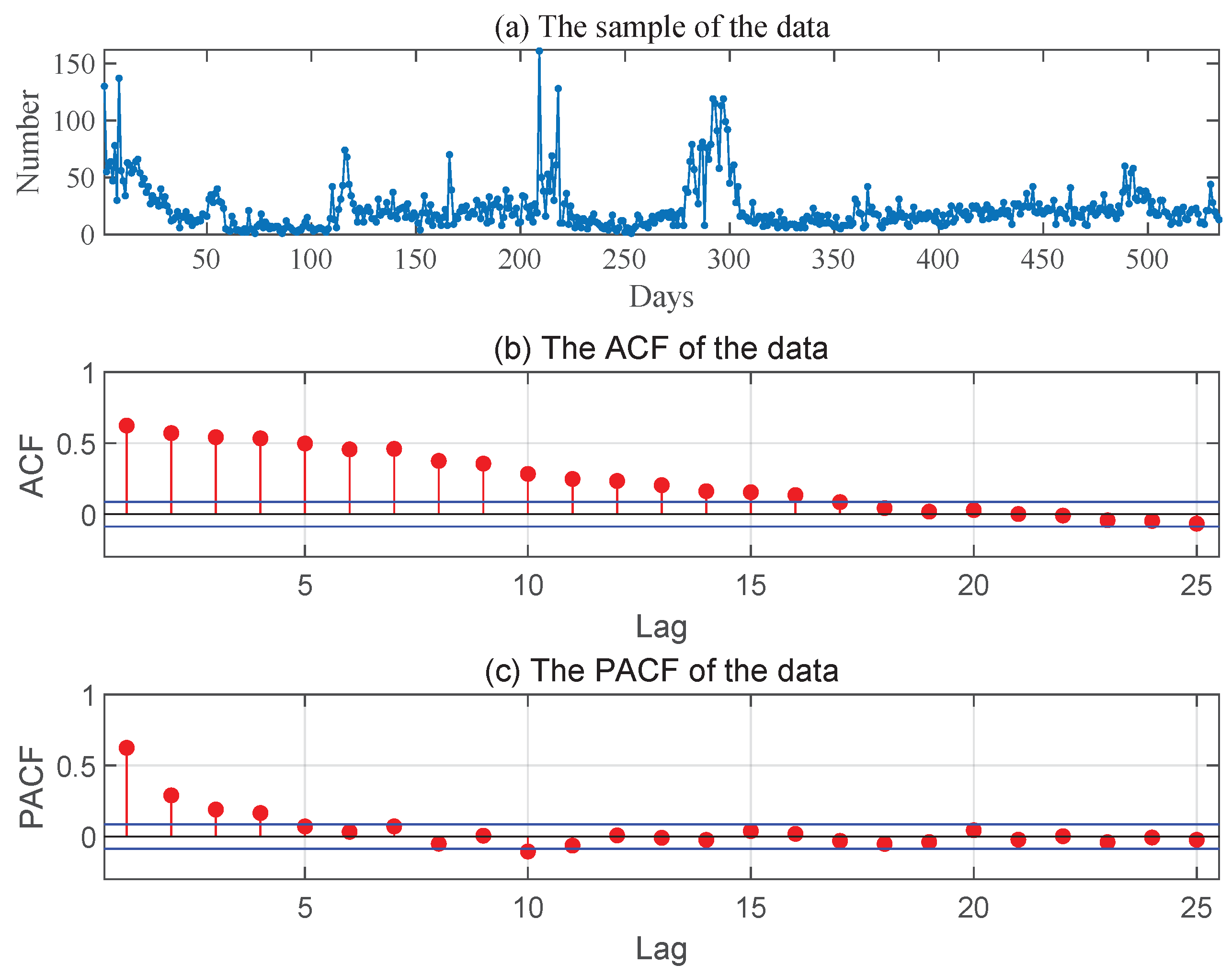
This data consist of the daily numbers of new asymptomatic COVID-19 cases in China, totally 534 observations (from 31 March to 15 September 2021) reported by the National Health Commission of the PRC. Figure 2 gives the sample path, the ACF and PACF of the series, from which it is reasonable for us to assume that these data come from an INAR(1) process.
We mainly apply the following four models to fit and analyze the data, among which the latter two models are considered here in order to show the superiority of the models constructed by the negative binomial thinning operator.
(1) NBRCINAR(1) process: the first-order random coefficient integer-valued autoregressive process constructed by the negative binomial thinning operator, i.e.,
in which .
(2) NBINAR(1) process: the first-order integer-valued autoregressive process with constant coefficient constructed by the negative binomial thinning operator, i.e.,
(3) BRCINAR(1) process: the first-order random coefficient integer-valued autoregressive process based on the binomial thinning operator, i.e.,
in which .
(4) BINAR(1) process: the first-order integer-valued autoregressive process with constant coefficient based on the binomial thinning operator, i.e.,
By using the method described in Section 4 to test the randomness of the thinning parameter, we obtain that the p-value is 0.0887, which suggests that we would reject the null hypothesis in favor of the alternative hypothesis at the significance level of , and thus, we should apply the NBRCINAR(1) process to fit the data.
To make further comparisons between the aforementioned four models, we split the data set into two parts: the first 529 observations from 31 March to 10 September are considered as a training sample to estimate the parameters, retaining the last 5 observations from 11 September to 15 September as a forecasting evaluation sample to perform an out-of-sample experiment. When estimating the parameters, the two-step CLS method makes it not necessary to specify the distribution of the innovation . Meanwhile, to improve the estimation performance, we use the block bootstrap method for the dependent time series proposed by Künsch [36] to derive the model parameters (1000 replications) and then obtain the CLS estimates by averaging the sample bootstrap estimates. Moreover, the forecasting performance of the estimated INAR models is assessed by the forecast mean absolute error (FMAE) statistics of h-step-ahead forecasts, which are defined by
where , , and is the coherent prediction of .
As for time series analysis, conditional expectation (CE for short) is the most common technique to construct forecasts, since it can lead to minimum mean squared error. However, for all the four models mentioned above, we have
which implies that we can not distinguish them because of the same CLS estimates of and . On the other hand, conditional expectation usually fails to preserve the integer-valued nature in making forecasts for count data time series. To cater these problems, Bisaglia and Gerolimetto [37] proposes a new approach based on the autoregressive structure of the INAR model by means of bootstrap techniques. We will also employ this method for further analysis. Taking the NBRCINAR(1) process as an example, the corresponding algorithm steps of this method are given as follows:
Step 1. Estimate the unknown model parameters of interest and by two-step CLS method to obtain and .
Step 2. Compute the residuals as
in which is a sequence of i.i.d. random variables drawn from Beta(,).
Step 3. Define the modified residuals as
and then fit the empirical distribution of .
Step 4. Obtain the bootstrapped series for by
where and are i.i.d. random samples from Beta(,) and , respectively.
Step 5. Based on the bootstrapped series , derive the estimators and of and as those in Step 1, respectively.
Step 6. Calculate the forecasts as
where H denotes the largest prediction horizon, , while and are i.i.d. random samples drawn from Beta(,) and , respectively.
Step 7. Obtain , the point forecast of by taking the median of the replicates for .
Table 6 presents the results of parameter estimation for the four different models we consider in this paper, i.e., the NBRCINAR(1) process (26), the NBINAR(1) process (27), the BRCINAR(1) process (28) and the BINAR(1) process (29). After applying the two-step CLS method, it can be seen that and in all the four models have the same estimates. In addition, the estimates of and in NBRCINAR(1) process and BRCINAR(1) process are also equal, respectively, which makes us dedicate ourselves to developing other estimation methods for these models. Furthermore, when using the model-based INAR bootstrap (MBB for short) technique to construct the forecasts, we set to achieve our goal for model selection, i.e., predict by MBB 501 times, choose the median of the obtained results as the value of , and then calculate the FMAE. According to the report in Table 7, it can be observed that the models with random coefficients outperform the models with a constant coefficient, which is consistent with the hypothesis testing result we have obtained. Additionally, under the same assumption for the thinning parameters, the models based on the negative binomial thinning operator work better than the models based on the binomial thinning operator, and the NBRCINAR(1) process has the best predictive performance. Therefore, we can conclude that our suggested model and method can be very helpful in some practical applications.
6.2. Poliomyelitis Data in USA
In this subsection, we turn to the data set that is comprised of the monthly number of poliomyelitis cases reported by the U.S. Centers for Disease Control. There are totally 168 observations, collected from January 1970 to December 1983. Figure 3 presents the sample path, the ACF and PACF of the time series. This data set has been used by Awale et al. [25] previously to test the constancy of the thinning parameter in a geometric INAR(1) models in which the distribution of the innovation is given. Now, we relax this condition and apply the NBRCINAR(1) process (26), the NBINAR(1) process (27), the BRCINAR(1) process (28) and the BINAR(1) process (29) without specifying to fit the Poliomyelitis data. With the method discussed in Section 4, we carried out the test for , and the p-value turns out to be 0.4960. Hence, the same conclusion as Awale et al. [25] can be reached, i.e, we can not reject the null hypothesis of the constant thinning parameter at the significance levels of and . In order to verify this assertion, we estimate the parameters of interest and list the results in Table 8. Moreover, the predicted values are shown in Table 9, from which it can be seen that the models with the constant coefficient are more appropriate than the models with random coefficients for this poliomyelitis data set.
7. Possibility for Expansions
To handle the variability in thinning parameters that may arise owing to numerous external or internal causes, this paper offers an integer-valued time series model based on the negative binomial thinning operator (the NBRCINAR(1) process) to analyze such count data and devises a technique to evaluate the thinning parameter’s constancy, which is very important for us to determine whether or not we should apply the model with random coefficients.
One of the advantages of the method discussed in this paper is that we need not specify the distribution of the innovation , so it is worthwhile to apply this method to other integer-valued time series models depending on the specific applications, to account for different circumstances or data features. Some straightforward and interesting generalizations for the NBRCINAR(1) process are as follows:
(1) The first-order generalized random coefficient integer-valued autoregressive (GRCINAR(1)) process proposed by Gomes and Canto [28], i.e.,
in which the generalized thinning operator is defined by
where represents a given discrete type distribution with mean and variance , respectively. It is obvious that the generalized thinning operator includes the binomial thinning operator, the negative binomial thinning operator, the expectation thinning operator and the Poisson thinning operator as its special cases.
(2) The first-order random coefficient mixed-thinning integer-valued autoregressive (RCMTINAR(1)) process was studied by Chang et al. [38], i.e.,
where the mixed thinning operator “” represents
in which is a counting series given as
with being a sequence of conditionally independent Bernoulli random variables, and , independent of given , being a sequence of conditionally independent Geometric random variables.
(3) The first-order random coefficients self-exciting integer-valued threshold autoregressive (RCTINAR(1)) process investigated by Yang et al. [18,21], i.e.,
in which “∘” is the binomial thinning operator, and r is the so-called threshold variable.
To test the randomness of the thinning parameters for these models, the attendant problem is how to estimate the parameter , or and , as well as establish the related asymptotic behaviors of the estimators. We will focus on these issues in the future study.
On the other hand, our model and method considered in this paper have some limitations and constraints, which also could provide many interesting future studies. Let us discuss several topics as follows:
(1) Our results heavily rely on the assumptions (A1)–(A4), which may restrict the usefulness and applicability of our method. Therefore, it needs more attention to extend the proposed method to the models that relax the condition of independence for practice. For example, we can introduce the Markov-switching mechanism for like Lu and Wang [39] and explore the random coefficient models with dependent counting series like Liu and Zhang [19], or with serially dependent innovations like Shirozhan and Mohammadpour [40].
(2) As we can see from the simulation results in Section 5, the estimates of , obtained in the second step of CLS method, converge to their true values at a slightly slow rate, and there is some gap between the empirical sizes and the designated significance levels for the test problems. Therefore, large sample sizes are needed to obtain good results. However, this requirement may be not met in practice. To improve the performance of statistical inference, we can apply the so-called locally most powerful-type test method developed by Awale et al. [25], but we have to fit the distribution of the innovation first. We can also try the empirical likelihood test method to obtain the estimators of model parameters, and then consider the constancy test of the thinning parameters, see Lu and Wang [26] for example.
8. Conclusions
In this paper, we consider the first-order random coefficient integer-valued autoregressive (NBRCINAR(1)) process based on the negative binomial thinning operator. We obtain the estimators of model parameters by the two-step conditional least squares method, and derive their asymptotic properties. We also consider the constancy test of thinning parameters. The simulation study demonstrates the effectiveness of our suggested method. The real data analysis reveals that our suggested method can be useful in practice. Finally, some possible extensions of this paper are provided. We leave these issues as our future work.
Funding
This paper is supported by National Natural Science Foundation of China (No. 12226506).
Data Availability Statement
The original data of asymptomatic COVID-19 cases in China presented in the study are openly available on the official website of National Health Commission of the PRC http://www.nhc.gov.cn/xcs/yqtb/list_gzbd.shtml. The Poliomyelitis data in USA presented in the study are available in Zeger [41].
Acknowledgments
The author would like to thank the editor and the three referees for their very constructive and pertinent suggestions that improve this paper a lot.
Conflicts of Interest
The author declares no conflicts of interest.
References
- Cox, D.R.; Miller, H.D. The Theory of Stochastic Processes; Methuen: London, UK, 1965. [Google Scholar]
- Jacobs, P.; Lewis, P. Stationary discrete autoregressive-moving average time series generated by mixtures. J. Time Ser. Anal. 1983, 4, 19–36. [Google Scholar] [CrossRef]
- Al-Osh, M.A.; Alzaid, A.A. First-order integer-valued autoregressive (INAR(1)) process. J. Time Ser. Anal. 1987, 8, 261–275. [Google Scholar] [CrossRef]
- Steutel, F.W.; van Harn, K. Discrete analogues of self-decomposability and stability. Ann. Probab. 1979, 7, 893–899. [Google Scholar] [CrossRef]
- Weiß, C.H. Thinning operations for modeling time series of counts—A survey. AStA Adv. Stat. Anal. 2008, 92, 319–343. [Google Scholar] [CrossRef]
- Scotto, M.G.; Weiß, C.H.; Gouveia, S. Thinning-based models in the analysis of integer-valued time series: A review. Stat. Model. 2015, 15, 590–618. [Google Scholar] [CrossRef]
- Weiß, C.H. An Introduction to Discrete-Valued Time Series; John Wiley and Sons Ltd.: Hoboken, NJ, USA, 2018. [Google Scholar]
- Weiß, C.H. Stationary count time series models. WIREs Comput. Stat. 2021, 13, e1502. [Google Scholar] [CrossRef]
- Ristić, M.M.; Bakouch, H.S.; Nastić, A.S. A new geometric first-order integer-valued autoregressive (NGINAR(1)) process. J. Stat. Plan. Inference 2009, 139, 2218–2226. [Google Scholar] [CrossRef]
- Ristić, M.M.; Nastić, A.S.; Bakouch, H.S. Estimation in an integer-valued autoregressive process with negative binomial marginals (NBINAR(1)). Commun. Stat.—Theory Methods 2012, 41, 606–618. [Google Scholar] [CrossRef]
- Yang, K.; Wang, D.H.; Jia, B.T.; Li, H. An integer-valued threshold autoregressive process based on negative binomial thinning. Stat. Pap. 2018, 59, 1131–1160. [Google Scholar] [CrossRef]
- Tian, S.Q.; Wang, D.H.; Cui, S. A seasonal geometric INAR process based on negative binomial thinning operator. Stat. Pap. 2020, 61, 2561–2581. [Google Scholar] [CrossRef]
- Wang, X.H.; Wang, D.H.; Yang, K.; Xu, D. Estimation and testing for the integer-valued threshold autoregressive models based on negative binomial thinning. Commun. Stat.—Simul. Comput. 2021, 50, 1622–1644. [Google Scholar] [CrossRef]
- Qian, L.Y.; Zhu, F.K. A new minification integer-valued autoregressive process driven by explanatory variables. Aust. N. Z. J. Stat. 2022, 64, 478–494. [Google Scholar] [CrossRef]
- Zheng, H.T.; Basawa, I.V.; Datta, S. Inference for pth-order random coefficient integer-valued autoregressive processes. J. Time Ser. Anal. 2006, 27, 411–440. [Google Scholar] [CrossRef]
- Zheng, H.T.; Basawa, I.V.; Datta, S. First-order random coefficient integer-valued autoregressive process. J. Stat. Plan. Inference 2007, 137, 212–229. [Google Scholar] [CrossRef]
- Zhang, H.X.; Wang, D.H.; Zhu, F.K. Empirical likelihood inference for random coefficient INAR(p) process. J. Time Ser. Anal. 2011, 32, 195–223. [Google Scholar] [CrossRef]
- Yang, K.; Li, H.; Wang, D.H.; Zhang, C.H. Random coefficients integer-valued threshold autoregressive processes driven by logistic regression. AStA Adv. Stat. Anal. 2021, 105, 533–557. [Google Scholar] [CrossRef]
- Liu, J.; Zhang, H.X. First-order random coefficient INAR process with dependent counting series. Commun. Stat.—Simul. Comput. 2022, 51, 3341–3354. [Google Scholar] [CrossRef]
- Li, H.; Liu, Z.J.; Yang, K.; Dong, X.G.; Wang, W.S. A pth-order random coefficients mixed binomial autoregressive process with explanatory variables. Comput. Stat. 2023. [Google Scholar] [CrossRef]
- Yang, K.; Li, A.; Yu, X.Y.; Dong, X.G. On MCMC sampling in random coefficients self-exciting integer-valued threshold autoregressive processes. J. Stat. Comput. Simul. 2024, 94, 164–182. [Google Scholar] [CrossRef]
- Yu, K.Z.; Tao, T.L. Consistent model selection procedure for random coefficient INAR models. Entropy 2023, 25, 1220. [Google Scholar] [CrossRef]
- Yu, M.J.; Wang, D.H.; Yang, K. A class of observation-driven random coefficient INAR(1) processes based on negative binomial thinning. J. Korean Stat. Soc. 2019, 48, 248–264. [Google Scholar] [CrossRef]
- Zhao, Z.W.; Hu, Y.D. Statistical inference for first-order random coefficient integer-valued autoregressive processes. J. Inequalities Appl. 2015, 2015, 359. [Google Scholar] [CrossRef]
- Awale, M.; Balakrishna, N.; Ramanathan, T.V. Testing the constancy of the thinning parameter in a random coefficient integer autoregressive model. Stat. Pap. 2019, 60, 1515–1539. [Google Scholar] [CrossRef]
- Lu, F.L.; Wang, D.H. A new estimation for INAR(1) process with Poisson distribution. Comput. Stat. 2022, 37, 1185–1201. [Google Scholar] [CrossRef]
- Nicholls, D.; Quinn, B. Random Coefficient Autoregressive Models: An Introduction; Springer: Berlin, Germany, 1982. [Google Scholar]
- Gomes, D.; Canto e Castro, L. Generalized integer-valued random coefficient for a first order structure autoregressive (RCINAR) process. J. Stat. Plan. Inference 2009, 139, 4088–4097. [Google Scholar] [CrossRef]
- Zhang, H.X.; Wang, D.H.; Zhu, F.K. Inference for INAR(p) processes with signed generalized power series thinning operator. J. Stat. Plan. Inference 2009, 140, 667–883. [Google Scholar] [CrossRef]
- Zheng, H.T.; Basawa, I.V. First-order observation-driven integer-valued autoregressive processes. Stat. Probab. Lett. 2008, 78, 1–9. [Google Scholar] [CrossRef]
- Hwang, S.; Basaea, I. Parameter estimation for generalized random coefficient autoregressive processes. J. Stat. Plan. Inference 1998, 68, 323–337. [Google Scholar] [CrossRef]
- Zhu, F.K.; Wang, D.H. Estimation of Parameters in the NLAR(p) Model. J. Time Ser. Anal. 2008, 29, 619–628. [Google Scholar] [CrossRef]
- Billingsley, P. The Lindeberg-Lévy theorem for martingales. Proc. Am. Math. Soc. 1961, 12, 788–792. [Google Scholar]
- Brockwell, P.J.; Davis, R.A. Time Series: Theory and Methods, 2nd ed.; Springer: New York, NY, USA, 1991. [Google Scholar]
- Karlsen, H.; Tjøstheim, D. Consistent estimates for the NEAR(2) and NLAR(2) time series models. J. R. Stat.-Soc.-Ser. B 1988, 50, 313–320. [Google Scholar] [CrossRef]
- Künsch, H. The Jackknife and the Boostrapt for general stationary observations. Ann. Stat. 1989, 17, 1217–1241. [Google Scholar] [CrossRef]
- Bisaglta, L.; Geroltmetto, M. Model-based INAR bootstrap for forecasting INAR(p) models. Comput. Stat. 2019, 34, 1815–1848. [Google Scholar] [CrossRef]
- Chang, L.Y.; Liu, X.F.; Wang, D.H.; Jing, Y.C.; Li, C.L. First-order random coefficient mixed-thinning integer-valued autoregressive model. J. Comput. Appl. Math. 2022, 410, 114222. [Google Scholar] [CrossRef]
- Lu, F.L.; Wang, D.H. First-order integer-valued autoregressive process with Markov-switching coefficients. Commun. Stat.—Theory Methods 2022, 51, 4313–4329. [Google Scholar] [CrossRef]
- Shirozhan, M.; Mohammadpour, M. A dependent counting INAR model with serially dependent innovation. J. Appl. Stat. 2021, 48, 1975–1997. [Google Scholar] [CrossRef]
- Zeger, S.L. A regression model for time series of counts. Biometrika 1988, 75, 621–629. [Google Scholar] [CrossRef]
Figure 1.
QQ plots of estimator .

Figure 2.
The sample path, ACF and PACF of the asymptomatic cases of COVID-19 in China.

Figure 3.
The sample path, ACF and PACF of the poliomyelitis data in USA.


Table 1.
Simulation results for and .
| n | Parameter | Parameter | ||||||
|---|---|---|---|---|---|---|---|---|
| Estimate | BIAS | MES | Estimate | BIAS | MSE | |||
| 100 | 0.4030 | −0.0970 | 0.0324 | 0.4096 | −0.0904 | 0.0286 | ||
| 0.0380 | −0.1703 | 0.0350 | 0.0529 | −0.1554 | 0.0338 | |||
| 1.1550 | 0.1550 | 0.0893 | 2.2974 | 0.2974 | 0.3045 | |||
| 300 | 0.4527 | −0.0473 | 0.0139 | 0.4550 | −0.0450 | 0.0127 | ||
| 0.0680 | −0.1403 | 0.0279 | 0.0875 | −0.1208 | 0.0235 | |||
| 1.0761 | 0.0761 | 0.0347 | 2.1435 | 0.1435 | 0.1260 | |||
| 500 | 0.4689 | −0.0311 | 0.0102 | 0.4749 | −0.0251 | 0.0086 | ||
| 0.0864 | −0.1219 | 0.0228 | 0.1085 | −0.0998 | 0.0179 | |||
| 1.0478 | 0.0478 | 0.0254 | 2.0895 | 0.0895 | 0.0942 | |||
| 1000 | 0.4789 | −0.0211 | 0.0059 | 0.4850 | −0.0150 | 0.0047 | ||
| 0.1149 | −0.0934 | 0.0157 | 0.1401 | −0.0682 | 0.0112 | |||
| 1.0387 | 0.0387 | 0.0159 | 2.0489 | 0.0489 | 0.0501 | |||
| 2000 | 0.4861 | −0.0139 | 0.0033 | 0.4928 | −0.0072 | 0.0028 | ||
| 0.1332 | −0.0751 | 0.0111 | 0.1597 | −0.0486 | 0.0068 | |||
| 1.0228 | 0.0228 | 0.0086 | 2.0265 | 0.0265 | 0.0308 | |||
| 5000 | 0.4965 | −0.0035 | 0.0015 | 0.4970 | −0.0030 | 0.0012 | ||
| 0.1649 | −0.0434 | 0.0054 | 0.1800 | −0.0283 | 0.0034 | |||
| 1.0044 | 0.0044 | 0.0044 | 2.0118 | 0.0118 | 0.0140 | |||
Table 2.
Simulation results for and .
| n | Parameter | Parameter | ||||||
|---|---|---|---|---|---|---|---|---|
| Estimate | BIAS | MES | Estimate | BIAS | MSE | |||
| 100 | 0.3179 | −0.0821 | 0.0290 | 0.3238 | −0.0762 | 0.0278 | ||
| 0.0258 | −0.1662 | 0.0314 | 0.0318 | −0.1602 | 0.0300 | |||
| 1.1072 | 0.1072 | 0.0566 | 2.2093 | 0.2093 | 0.2294 | |||
| 300 | 0.3622 | −0.0378 | 0.0120 | 0.3694 | −0.0306 | 0.0119 | ||
| 0.0531 | −0.1380 | 0.0249 | 0.0629 | −0.1291 | 0.0230 | |||
| 1.0480 | 0.0480 | 0.0219 | 2.0892 | 0.0892 | 0.0905 | |||
| 500 | 0.3712 | −0.0288 | 0.0087 | 0.3778 | −0.0222 | 0.0080 | ||
| 0.0597 | −0.1323 | 0.0227 | 0.0760 | −0.1160 | 0.0192 | |||
| 1.0421 | 0.0421 | 0.0174 | 2.0573 | 0.0573 | 0.0604 | |||
| 1000 | 0.3830 | −0.0170 | 0.0055 | 0.3859 | −0.0141 | 0.0043 | ||
| 0.0836 | −0.1084 | 0.0176 | 0.1045 | −0.0875 | 0.0129 | |||
| 1.0227 | 0.0227 | 0.0108 | 2.0386 | 0.0386 | 0.0353 | |||
| 2000 | 0.3925 | −0.0075 | 0.0029 | 0.3954 | −0.0046 | 0.0025 | ||
| 0.1056 | −0.0864 | 0.0121 | 0.1271 | −0.0649 | 0.0082 | |||
| 1.0105 | 0.0105 | 0.0061 | 2.0122 | 0.0122 | 0.0201 | |||
| 5000 | 0.3970 | −0.0030 | 0.0013 | 0.3978 | −0.0022 | 0.0011 | ||
| 0.1387 | −0.0533 | 0.0063 | 0.1492 | −0.0428 | 0.0044 | |||
| 1.0037 | 0.0037 | 0.0027 | 2.0059 | 0.0059 | 0.0091 | |||
Table 3.
Simulation results for and .
| n | Parameter | Parameter | ||||||
|---|---|---|---|---|---|---|---|---|
| Estimate | BIAS | MES | Estimate | BIAS | MSE | |||
| 100 | 0.4920 | −0.1080 | 0.0343 | 0.5084 | −0.0916 | 0.0291 | ||
| 0.0532 | −0.1388 | 0.0292 | 0.0822 | −0.1098 | 0.0275 | |||
| 1.2004 | 0.2004 | 0.1267 | 2.3671 | 0.3671 | 0.4273 | |||
| 300 | 0.5428 | −0.0572 | 0.0140 | 0.5542 | −0.0458 | 0.0108 | ||
| 0.0921 | −0.0999 | 0.0215 | 0.1186 | −0.0734 | 0.0184 | |||
| 1.1124 | 0.1124 | 0.0538 | 2.1917 | 0.1917 | 0.1665 | |||
| 500 | 0.5615 | −0.0385 | 0.0096 | 0.5714 | −0.0286 | 0.0075 | ||
| 0.1046 | −0.0874 | 0.0183 | 0.1356 | −0.0564 | 0.0146 | |||
| 1.0732 | 0.0732 | 0.0358 | 2.1285 | 0.1285 | 0.1184 | |||
| 1000 | 0.5615 | −0.0385 | 0.0096 | 0.5793 | −0.0207 | 0.0044 | ||
| 0.1338 | −0.0582 | 0.0136 | 0.1532 | −0.0388 | 0.0101 | |||
| 1.0446 | 0.0446 | 0.0222 | 2.0824 | 0.0824 | 0.0693 | |||
| 2000 | 0.5851 | −0.0149 | 0.0030 | 0.5924 | −0.0076 | 0.0022 | ||
| 0.1496 | −0.0424 | 0.0093 | 0.1623 | −0.0297 | 0.0073 | |||
| 1.0276 | 0.0276 | 0.0117 | 2.0362 | 0.0362 | 0.0390 | |||
| 5000 | 0.5939 | −0.0061 | 0.0014 | 0.5956 | −0.0044 | 0.0009 | ||
| 0.1664 | −0.0256 | 0.0056 | 0.1739 | −0.0181 | 0.0041 | |||
| 1.0130 | 0.0130 | 0.0060 | 2.0191 | 0.0191 | 0.0161 | |||
Table 4.
Empirical power of the test at significance levels and .
| Level | Parameter | 10,000 | |||||
|---|---|---|---|---|---|---|---|
| 0.10 | 0.248 | 0.302 | 0.462 | 0.652 | 0.902 | 0.973 | |
| 0.256 | 0.432 | 0.639 | 0.812 | 0.962 | 0.990 | ||
| 0.233 | 0.271 | 0.302 | 0.475 | 0.812 | 0.943 | ||
| 0.208 | 0.258 | 0.440 | 0.748 | 0.923 | 0.983 | ||
| 0.284 | 0.374 | 0.484 | 0.633 | 0.858 | 0.968 | ||
| 0.303 | 0.459 | 0.599 | 0.745 | 0.948 | 0.999 | ||
| 0.05 | 0.158 | 0.234 | 0.393 | 0.577 | 0.844 | 0.945 | |
| 0.172 | 0.357 | 0.552 | 0.738 | 0.923 | 0.975 | ||
| 0.130 | 0.150 | 0.200 | 0.370 | 0.699 | 0.890 | ||
| 0.122 | 0.178 | 0.314 | 0.520 | 0.857 | 0.967 | ||
| 0.210 | 0.309 | 0.410 | 0.536 | 0.767 | 0.943 | ||
| 0.237 | 0.398 | 0.500 | 0.638 | 0.893 | 0.975 |
Table 5.
Empirical size of the test at significance levels and .
| Level | Parameter | 10,000 | 20,000 | |||||
|---|---|---|---|---|---|---|---|---|
| 0.10 | 0.037 | 0.033 | 0.034 | 0.031 | 0.038 | 0.045 | 0.057 | |
| 0.037 | 0.029 | 0.033 | 0.048 | 0.049 | 0.058 | 0.065 | ||
| 0.033 | 0.033 | 0.042 | 0.037 | 0.043 | 0.042 | 0.059 | ||
| 0.037 | 0.028 | 0.033 | 0.048 | 0.049 | 0.058 | 0.063 | ||
| 0.039 | 0.043 | 0.035 | 0.039 | 0.043 | 0.040 | 0.052 | ||
| 0.036 | 0.032 | 0.027 | 0.032 | 0.043 | 0.048 | 0.065 | ||
| 0.05 | 0.021 | 0.022 | 0.012 | 0.011 | 0.015 | 0.017 | 0.026 | |
| 0.020 | 0.014 | 0.016 | 0.025 | 0.019 | 0.027 | 0.031 | ||
| 0.019 | 0.015 | 0.016 | 0.017 | 0.015 | 0.015 | 0.023 | ||
| 0.022 | 0.014 | 0.016 | 0.025 | 0.019 | 0.027 | 0.034 | ||
| 0.028 | 0.013 | 0.015 | 0.017 | 0.013 | 0.015 | 0.027 | ||
| 0.017 | 0.017 | 0.012 | 0.005 | 0.014 | 0.016 | 0.023 |
Table 6.
Estimate of parameters in the models for the asymptomatic cases of COVID-19 in China.
| Parameters | ||||
|---|---|---|---|---|
| Model | ||||
| NBINAR(1) and BINAR(1) | 0.5788 | - | - | 9.3869 |
| NBRCINAR(1) and BRCINAR(1) | 0.5788 | 2.5027 | 1.8209 | 9.3869 |
Table 7.
Forecasting performance results for the asymptomatic cases of COVID-19 in China.
| Date | 1 September | 2 September | 3 September | 4 September | 5 September | FMAE |
|---|---|---|---|---|---|---|
| Observations | 44 | 28 | 20 | 16 | 13 | - |
| Forecast-CE | 21.5425 | 21.8565 | 22.0382 | 22.1434 | 22.2043 | 9.1974 |
| Forecast-MBB for NBRCINAR(1) | 19 | 20 | 19 | 18 | 19 | 8.4000 |
| Forecast-MBB for NBINAR(1) | 18 | 19 | 19 | 19 | 20 | 9.2000 |
| Forecast-MBB for BRCINAR(1) | 19 | 19 | 19 | 19 | 19 | 8.8000 |
| Forecast-MBB for BINAR(1) | 17 | 17 | 18 | 18 | 18 | 9.4000 |
Table 8.
Estimate of parameters in the models for the poliomyelitis data in USA.
| Parameters | ||||
|---|---|---|---|---|
| Model | ||||
| NBINAR(1) and BINAR(1) | 0.2540 | - | - | 0.9720 |
| NBRCINAR(1) and BRCINAR(1) | 0.2540 | 2.2654 | 6.6521 | 0.9720 |
Table 9.
Forecasting performance results for the poliomyelitis dat in USA.
| Time | August 1983 | September 1983 | October 1983 | November 1983 | December 1983 | FMAE |
|---|---|---|---|---|---|---|
| Observations | 1 | 0 | 1 | 3 | 6 | - |
| Forecast-CE | 1.4767 | 1.3442 | 1.3106 | 1.3021 | 1.2999 | 1.7059 |
| Forecast-MBB for NBRCINAR(1) | 1 | 1 | 1 | 1 | 1 | 1.6000 |
| Forecast-MBB for NBINAR(1) | 2 | 1 | 1 | 2 | 2 | 1.4000 |
| Forecast-MBB for BRCINAR(1) | 1 | 2 | 1 | 1 | 1 | 1.8000 |
| Forecast-MBB for BINAR(1) | 1 | 1 | 1 | 1 | 1 | 1.6000 |
Disclaimer/Publisher’s Note: The statements, opinions and data contained in all publications are solely those of the individual author(s) and contributor(s) and not of MDPI and/or the editor(s). MDPI and/or the editor(s) disclaim responsibility for any injury to people or property resulting from any ideas, methods, instructions or products referred to in the content. |
© 2024 by the author. Licensee MDPI, Basel, Switzerland. This article is an open access article distributed under the terms and conditions of the Creative Commons Attribution (CC BY) license (https://creativecommons.org/licenses/by/4.0/).
Share and Cite
MDPI and ACS Style
Zhang, S. Randomness Test of Thinning Parameters for the NBRCINAR(1) Process. Axioms 2024, 13, 260. https://doi.org/10.3390/axioms13040260
AMA Style
Zhang S. Randomness Test of Thinning Parameters for the NBRCINAR(1) Process. Axioms. 2024; 13(4):260. https://doi.org/10.3390/axioms13040260
Chicago/Turabian StyleZhang, Shuanghong. 2024. "Randomness Test of Thinning Parameters for the NBRCINAR(1) Process" Axioms 13, no. 4: 260. https://doi.org/10.3390/axioms13040260
Note that from the first issue of 2016, this journal uses article numbers instead of page numbers. See further details here.