Research on the Optimization of Pricing and the Replenishment Decision-Making Problem Based on LightGBM and Dynamic Programming

Abstract

Vegetables have a short period of freshness, and therefore, the purchase of vegetables has to be carefully matched with sales, especially in the “small production and big market” setting prevalent in China. Therefore, it is worthwhile to develop a systematic and comprehensive mathematical model of replenishment plans and pricing strategies for each category of vegetables and individual products. In this paper, we analyze the following three questions: Question One: What is the distribution law and relationship between the sales volume of vegetable categories and single products? Question Two: What is the relationship between total sales volume and cost-plus pricing of vegetable categories? And is it possible to provide the daily total replenishment and pricing strategy of each vegetable category for the following week to maximize supermarket profit? Question Three: How can we incorporate the market demand for single vegetable products into a profit-maximizing program for supermarkets? Is it possible to further formulate the replenishment plan requirements for single products? To answer the first question, we created pivot tables to analyze occupancy. We found that mosaic leaves, peppers, and edible mushrooms accounted for a larger proportion of occupacy, while cauliflowers, aquatic rhizomes, and eggplants accounted for a smaller proportion. For the single items, lettuce, cabbage, green pepper, screw pepper, enoki mushroom, and shiitake mushroom accounted for a large proportion of their respective categories. We used the Pearson correlation coefficient and the Mfuzz package based on fuzzy c-means (FCM) algorithm to analyze the correlation between vegetable categories and single products. We found that there was a strong correlation between vegetable categories. Moreover, the sale of vegetable items belonging to the same category exhibited the same patterns of change over time. In order to address the second question, we established the LightGBM sales forecasting model. Combined with previous sales data, we forecasted and planned an efficient daily replenishment volume for each vegetable category in the coming week. In addition, we developed a pricing strategy for vegetable categories to maximize supermarket profits. For the third question, we built a dynamic programming model combining an optimal replenishment volume with a product pricing strategy for single items, which let the supermarket maximize its expected profits.

1. Introduction

The quality of vegetable products in fresh food stores declines as the time to sale increases. Most varieties cannot be sold on the first day, and it is difficult to sell them on the following day, which also requires a price reduction. In order to mitigate losses, retailers have to decide whether to replenish each vegetable category on a daily basis, even if they are unsure of the specific single product and purchase price [1]. The production cycle of vegetables and the volatility of vegetable prices are unavoidable economic phenomena that cause vegetable prices to fluctuate dramatically and affect the harmony and stability of society and the daily lives of the population. They also represent a severe challenge to the healthy operation of the social economy [2]. Currently, the “cost-plus pricing” method is generally used to determine the price of vegetables [3].

In 2002, while studying the core ideas of dynamic programming, Zhu et al. [4] concluded that it is essential to identify states that can be used as state transitions and actions that can be used as decisions. In 2007, Yang et al. [5] resolved the development process of the fuzzy c-means (FCM) algorithm, which is a clustering method for processing gene expression or protein expression profiling data. This method can also identify underlying time-series patterns in expression profiles and divide factors with similar patterns into clusters. In 2010, Lu [6] studied the importance of fresh vegetable selling prices to supermarkets’ operations in relation to such commodities. He proposed a new dynamic pricing method, i.e., the value loss pricing method, for the handling of high-quality fresh vegetables. In 2012, Yan et al. [7] introduced state variables and decision variables to solve the problem of how to define the state transition equation. In 2014, Wang [8] used case studies, field research, interviews, econometric analyses, and other methods and drew the following conclusions: vegetable retailers generally adopt a psychological pricing strategy in which the markup of expensive vegetables is significantly higher than that of cheaper vegetables; on the other hand, consumers’ sense of price fairness can, in turn, significantly affect vegetable retail prices. In 2015, Song [9] made a specific analysis of the current situation and existing problems of vegetable supply chain inventory management in Shouguang City and proposed an optimization model for inventory management of the vegetable supply chain. In 2020, Wu [10] proposed the state transition function as a useful tool to describe the evolution of the state variables and introduced the specific mathematical expression of this function. In 2021, Lu et al. [11] proposed an optimizable replenishment strategy based on the dynamic matrix model for different application scenarios and demands in traditional retail to achieve on-demand intelligent replenishment. In 2022, Feng et al. [12] studied the data-fitting problem in relation to monomial polynomials and used the least squares method to minimize the residuals of the fit curve and data points to solve application problems. In 2023, Li [13] investigated the equilibrium relationship between freshness technology investment and product inventory, pricing, and revenue and proposed an exponential function of the spoilage rate associated with freshness technology investment under the premise of a multi-product joint replenishment strategy. In 2023, Xie et al. [14] studied LightGBM, which is an improved model based on decision tree and gradient boosting models, and used this model to solve various classification and regression problems. In 2024, Xu et al. [15] classified the inventory commodities of a trading company, selected the best method of classification by comparison, and formulated a corresponding inventory management strategy.

Scholars and experts have come to their own conclusions about automatic pricing and replenishment decisions in relation to vegetable products; however, there are still some factors that have not been taken into account. In this paper, we address the following three questions:

Question One: What is the distribution law and relationship between the sales volume of vegetable categories and single products?

Question Two: What is the relationship between total sales volume and cost-plus pricing of vegetable categories? And is it possible to provide the daily total replenishment and pricing strategy of each vegetable category for the following week to maximize supermarket profit?

Question Three: How can we incorporate the market demand for vegetable single products into the profit-maximizing program for supermarkets? Is it possible to further formulate the replenishment plan’s requirements for single products?

The three questions are not independent and are interrelated. If we want to explore how to develop a replenishment plan and pricing strategy for vegetable categories, we must first have a general understanding of the distribution law and the relationship between vegetable categories and items. After formulating the replenishment plan and pricing strategy for vegetable categories, it was natural for us to think of subdividing the research object from vegetable categories to vegetable items. According to the requirements of the market, we added constraints and further formulated the replenishment plan and pricing strategy of single vegetable items on the basis of the vegetable categories, so that supermarkets could obtain maximum profit.

To answer the first question, we created pivot tables to analyze occupancy. We found that mosaic leaves, peppers, and edible mushrooms accounted for a larger proportion, while cauliflowers, aquatic rhizomes, and eggplants accounted for a smaller proportion. For single items, lettuce, cabbage, green pepper, screw pepper, enoki mushroom, and shiitake mushroom accounted for a large proportion of their respective categories. We used the Pearson correlation coefficient and the Mfuzz package based on the fuzzy c-means (FCM) algorithm to analyze the correlation between vegetable categories and single products. We found that there was a strong correlation between vegetable categories. Moreover, the sales of vegetable items belonging to the same category exhibited the same patterns of change over time. In order to address the second question, we established the LightGBM sales forecasting model. Combined with previous sales data, we forecasted and planned an efficient daily replenishment volume for each vegetable category in the coming week. In addition, we developed a pricing strategy for vegetable categories to maximize supermarket profits. For the third question, we built a dynamic programming model combining an optimal replenishment volume with a product pricing strategy for single items, which let the supermarket maximize its expected profits.

In this study, we combined the impact of seasonal factors on the sales situation and used previous sales data to establish a scientific and effective mathematical model. This model provides a theoretical basis for the reasonable prediction of the sales of various categories of vegetables and individual products. We used it to develop a reasonable replenishment and pricing strategy. Our model is of great significance for reducing resource waste and environmental pollution, maximizing retailer profits, and promoting the sustainable development of the vegetable industry.

2. Basic Assumptions and Data Pre-Processing

2.1. Basic Assumptions

In this study, we made the following assumptions:

(1)

The vegetable items in the annex were sold on the same day and not on the next day;

(2)

Vegetables with different supply sources but the same individual item name in the annex were considered to be the same individual item;

(3)

The current day’s sales data for a single vegetable item approximated the previous day’s sales data;

(4)

Vegetable sales were independent of whether or not they were discounted.

2.2. Data Pre-Processing

In this paper, we pre-processed the data using Python, including data consolidation, outlier handling, and missing value processing.

2.2.1. Data Consolidation

To simplify the study, we processed the data as follows:

Step 1: Based on days, the sales volume of products with the same item code on the same day was computed. To simplify the research, we ignored the impact of product discounts and used the maximum sales unit price of the same item on the same day as the unit price of this item.

Step 2: We assumed that vegetables not sold on the same day could not then be sold the following day. We processed the “Sales Date” and “Date” columns together as the “Sales Date” since their meanings are the same. In addition, we deleted the data on unpurchased vegetable products since vegetables that had not been restocked could not be sold the next day. We merged the data according to whether they had the same values of “Sales Date” and “Item Code”.

Step 3: Firstly, we further merged the merged data according to the “Item Code” field. Secondly, we ignored the fields “Sales Type”, “Discounted or Not”, “Sweep Code Sales Time”, and “Classification Code” since they had low relevance to the study subject. Lastly, we generated a new field “Profit Margin” to better describe supermarket revenue.

Part of the processed data is shown in

Table 1. Selected data display tables for processing.

Item Name	Amaranth Greens (Amaranthus)	Yunnan Lettuce	Brussels Sprouts (Brassica oleracea)	Brassica Chinensis	Shanghai Youth
Product Code	10290000	10290000	10290000	10290000	10290000
	5115762	5115779	5115786	5115793	5115823
Single-Variety Category	Philodendron	Philodendron	Philodendron	Philodendron	Philodendron
Date of Sale	1 July 2020	1 July 2020	1 July 2020	1 July 2020	1 July 2020
Daily Sales (kg)	6.841	41.966	11.352	4.288	11.476
Selling Unit Price (CNY/kg)	6	8	6	16	10
Wholesale Price (CNY/kg)	3.88	6.72	3.19	9.24	7.03
Profitability (%)	54.64	19.05	88.09	73.16	42.25
Loss Rate (%)	18.52	15.25	13.62	7.59	14.43

.

2.2.2. Outlier Handling

We assumed that vegetables not sold on the same day could not then be sold the next day. In addition, we removed data values for which daily sales were less than 0. Since neither the “Sales Unit Price (yuan/kg)” nor the “wholesale price (yuan/kg)” could be directly judged as outliers, we used “Profit Margin (%)” as an indicator to determine whether the data were abnormal. In this study, we used a box plot to detect outliers in the logarithmically transformed “Sales Volume (kg)” and “Profit Margin (%)” data. Combined with the box plots (e.g., Figure 1 and Figure 2), we found and deleted data that contained anomalous values.

2.2.3. Missing Value Processing

Since there were missing data on daily total sales for certain vegetable categories, we used the sliding time window analysis to fill the vacant data. Firstly, we used multiple time segments of information and set them as a window that always maintained the total unchanged value of the time period. When the data were updated, the window contained the data for the latest time period. Secondly, we defined the data time interval series as $\left[T_0,T_1,T_2,\cdots ,T_n\right]$ and set the time intervals to be equal in length. Lastly, we set $\left[T_i,T_{i+1},T_{i+2},\cdots ,T_{i+n}\right]$ to be a sliding window, where i was an integer that was not less than 0 and $T_i$ represented the time interval between time $t_{i-1}$ and time $t_i$. As shown in Figure 3, when the window advanced to the next time interval, the data were updated, thus filling the vacant data.

3. Solution to Question One

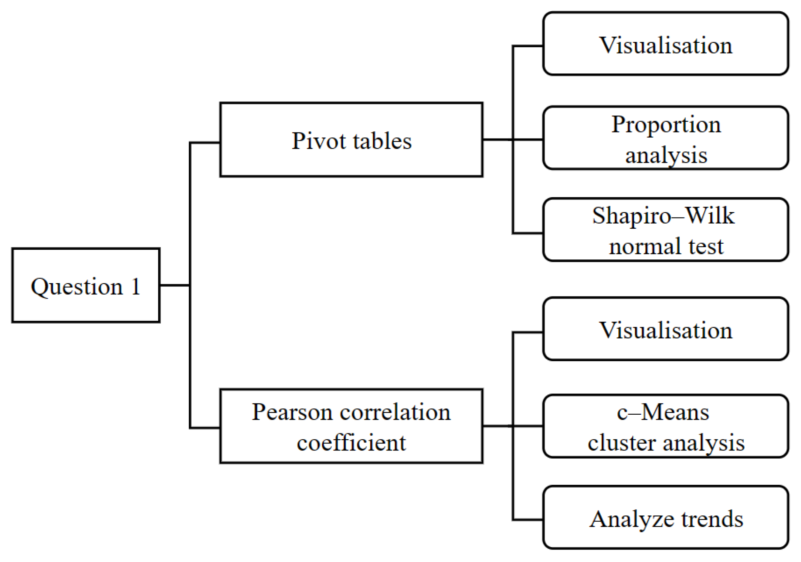
3.1. Research Ideas

Firstly, since the sales volume of each category and individual item of vegetable goods is a continuous variable, we calculated the total sales of each category and individual item using a pivot table and analyzed the percentage situation. Secondly, we used the Shapiro–Wilk test on the total sales volume data of each category and individual item to check whether the data had a normal distribution or not. Thirdly, we used the Pearson correlation coefficient to calculate the interrelationship between the total sales of each vegetable category and further investigated the correlation using a heat map. Finally, since the total sales volume of individual items is greatly affected by season, in order to better study the interrelationship between the sales volume of individual items, we used the Mfuzz package based on the fuzzy c-means (FCM) algorithm to perform a cluster analysis of the normalized monthly sales volume of a single item on an annual basis. In order to illustrate our thinking, a flowchart is shown in Figure 4.

3.2. Preparation

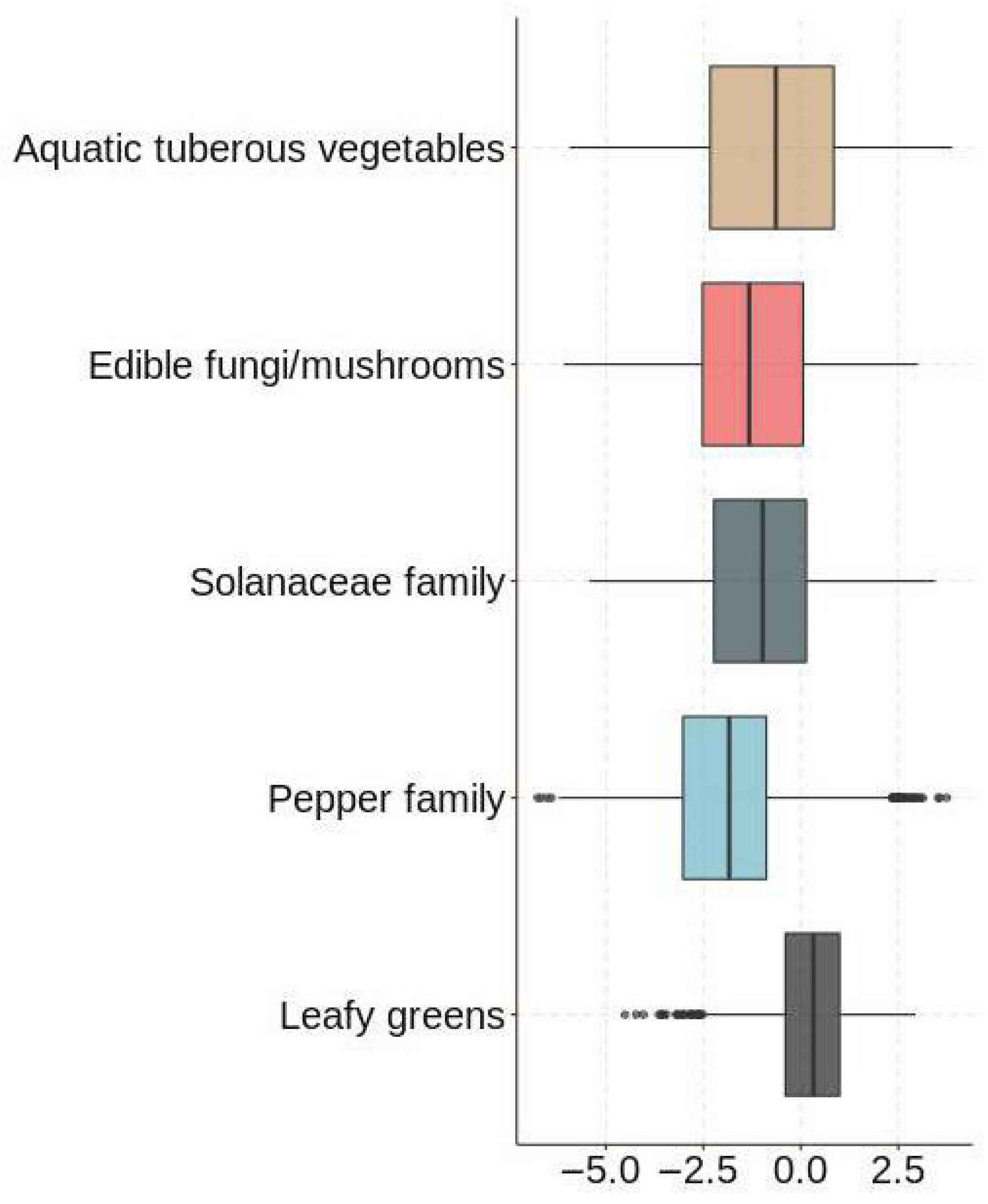
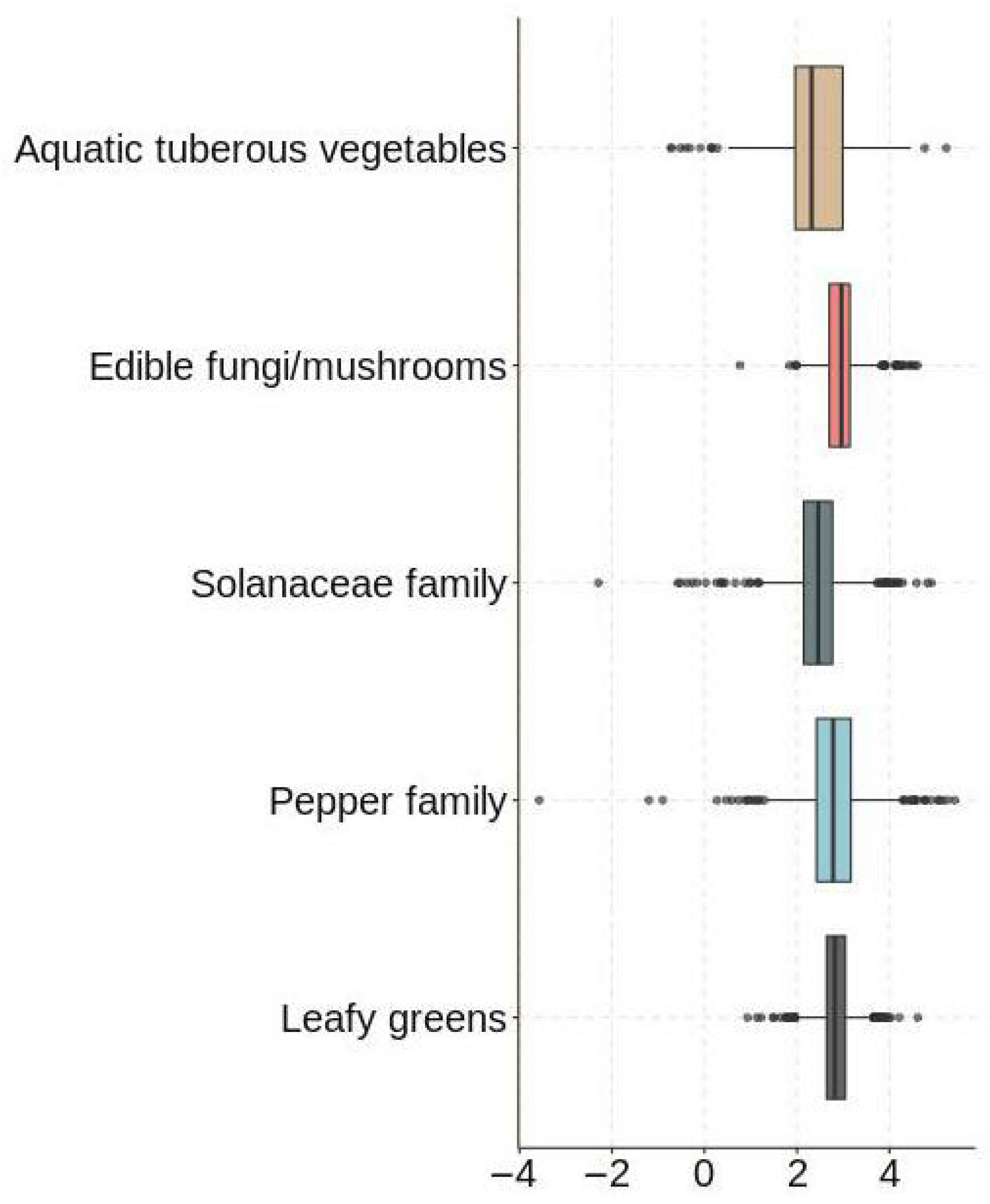
3.2.1. Visualization and Analysis of Data

After merging the data and eliminating the outliers, a pivot table was established with the help of Python to calculate the total sales of each category and single product. Then, we analyzed the percentage situation and visualized it. Because there were too many types of single items in certain vegetable categories, only the top three items in each category were selected and recorded in the table. The statistical results of the proportions of total sales are shown in

Table 2. Category and unit sales share statistics from 2020-07 to 2022-06.

Vegetable Category	Total Sales Volume by Category (kg)	Percentage of Total	Single Vegetables	Total Sales of Individual Products (kg)	Percentage Share	Percentage of Total
Philodendron	197,395	42.15%	Yunnan Lettuce	30,177	15.29%	6.44%
			Brassica Pekinensis	19,100	9.68%	4.08%
			Yunnan Oilseed Rape (Brassica napus)	19,081	9.66%	4.07%
Capsicum	90,561	19.34%	Wuhu Green Pepper	27,628	30.51%	5.9%
			King Cobra or Chili (Naga Jolokia)	15,893	17.55%	3.39%
			Chili	12,185	11.87%	2.61%
Edible Mushroom	75,909	16.21%	Enoki Mushroom	23,411	30.8%	5.01%
			Xixia Shiitake Mushroom	11,910	15.68%	2.54%
			Agaricus Bisporus (Botany)	4228	5.57%	0.9%
Cauliflower (Brassica oleracea var. botrytis)	41,667	8.9%	Broccoli	27,502.53	66.0%	5.87%
			Chinese Green Stem with Scattered Flowers	8339.201	20.01%	1.78%
			Zijiang Qingdian Scattered Flowers	5811.909	13.95%	1.24%
Aquatic Rhizomes	40,466	8.64%	Net Lotus Root	27,105.79	66.98%	5.79%
			Lotus Root	6034	14.91%	1.29%
			Lotus Seedling (Pcs)	2075	5.13%	0.44%
Eggplant	22,361	4.77%	Purple Eggplant (Solanum melongena L.)	13,856	61.97%	2.96%
			Eggplant (Solanum melongena L.)	3687	15.66%	0.79%
			Long-Term Eggplant	2493.227	11.15%	0.53%

.

It can be observed from Table 2 that philodendron, capsicum, and edible mushrooms accounted for a larger proportion, and there were many types of single items in these categories. Among them, lettuce, cabbage, green pepper, screw pepper, enoki mushroom, and shiitake mushroom accounted for a large proportion of their respective categories. Moreover, cauliflowers, aquatic rhizomes, and eggplants accounted for a small proportion, and their types of single items were relatively simple.

3.2.2. Statistical Tests

For the statistical tests, we used the Pearson correlation coefficient to quantitatively analyze the interrelationship between the total sales of each category. An explanation of the Pearson correlation coefficient can be found in [16]. The use of the Pearson correlation coefficient not only required a linear correlation between the two variables but also required them to obey a normal distribution.

Since the sample totals of the data to be tested were very small, we selected the Shapiro–Wilk test to assess their normality. The results of the test are shown in

Table 3. Statistical tests’ results for vegetable categories.

Vegetable Category	Upper Quartile	Average Value	Standard Deviation	Skewness	Kurtosis	S–W Test	p-Value
Philodendron	186.329	2035.007	3626.467	2.507	7.096	0.628	0.988
Capsicum	368.459	2106.073	4804.619	4.038	19.248	0.475	0.761
Edible Mushroom	212.171	1100.134	2467.288	4.407	22.079	0.465	0.197
Cauliflower (Brassica oleracea var. botrytis)	5811.909	8333.502	11,318.942	1.687	3.017	0.803	0.304
Aquatic Rhizomes	232.403	2248.137	6369.707	3.916	15.852	0.389	0.311
Eggplant	1047.247	2484.639	4321.602	2.595	7.086	0.620	0.514

.

It can be seen from Table 3 that the p-value of each vegetable category was greater than 0.05, and the sales volume of each individual item in each vegetable category conformed to a normal distribution. Thus, these data were deemed ready for the next step: the Pearson coefficient linear correlation analysis.

3.3. Modeling and Solving

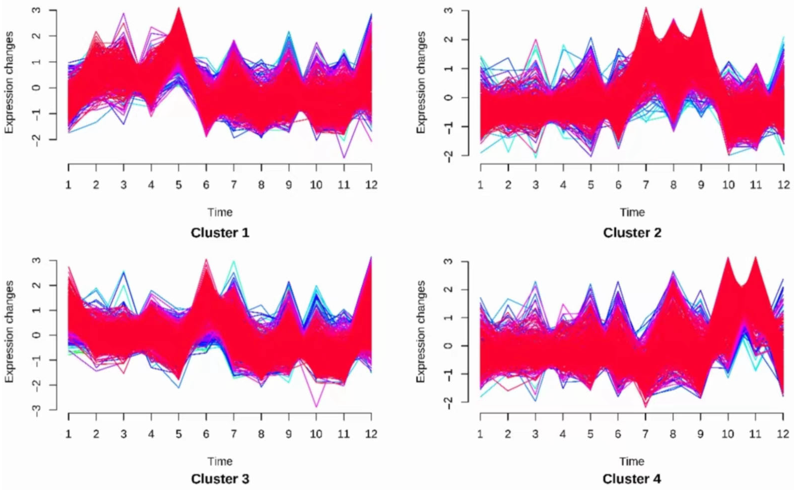
3.3.1. Establishing and Solving the Category Sales Volume Correlation Model

To explore the interrelationship between the sales volume of vegetable categories, we calculated the Pearson correlation coefficient with the help of Python for the qualitative analysis. The specific values are shown in

Table 4. Analysis results of Pearson’s correlation coefficient between the sales volume of vegetable categories.

	Aquatic Rhizomes	Philodendron	Cauliflower (Brassica oleracea var. botrytis)	Eggplant	Capsicum	Edible Mushroom
Aquatic rhizomes	1	0.637374104	0.796073285	0.595787529	0.808103253	0.684693022
Philodendron	0.637374104	1	0.713041043	0.54202519	0.640759134	0.542313018
Cauliflower (Brassica oleracea var. botrytis)	0.796073285	0.713041043	1	0.62882682	0.592117531	0.506056629
Eggplant	0.595787529	0.54202519	0.62882682	1	0.742529242	0.600157973
Capsicum	0.808103253	0.640759134	0.592117531	0.742529242	1	0.598800308
Edible Mushroom	0.684693022	0.542313018	0.506056629	0.600157973	0.598800308	1

.

As can be seen from Table 4, the interval range of the correlation coefficient values obtained was $[0.5060,0.8081]$, and there was a linear correlation between the sales volume of each category.

3.3.2. Establishing and Solving the Single Product Sales Volume Correlation Model

Since single-item sales were more likely to vary as a result of seasonal influences than vegetable categories, we used the Mfuzz package in Python based on the fuzzy c-means (FCM) algorithm to perform a cluster analysis of the normalized monthly sales volume for each single item.

A single data point can belong to multiple clusters, and the core idea of the fuzzy c-means (FCM) algorithm is to divide n data points into k fuzzy clusters and find the center of each cluster to minimize the value of the objective function. Therefore, let $X=\left\{x_1,x_2,\cdots ,x_n\right\}$ be n data samples. In addition, let c be the number of data sample classifications with a value in the range $2\le c\le n$. Moreover, let $\left\{A_1,A_2,\cdots ,A_c\right\}$ be the corresponding c categories, and let U be the similarity classification matrix. Finally, let $\left\{v_1,v_2,\cdots ,v_c\right\}$ be the clustering center of each category, and let ${\mu }_{\mathrm{k}}\left(x_i\right)$ be the degree of affiliation of samples $x_i$ to class $A_{\mathrm{k}}$ (abbreviated as ${\mu }_{\mathrm{ik}}$). Thus, the objective function $J_{\mathrm{b}}$ is as follows:

$$J_b(\mathbf{U},v)=\sum _{i=1}^n\sum _{k=1}^c{\left({\mu }_{ik}\right)}^b{\left(d_{ik}\right)}^2,$$

where b is a weighting parameter with a value in the range $1\le b<\infty$, and $d_{ik}$ is the distance between $x_i$ and the centroid of the k class in the i sample

$$d_{ik}=d\left(x_i-v_k\right)=\sqrt{\sum _{j=1}^m{\left(x_{ij}-v_{kj}\right)}^2},$$

where m is the number of sample features. The fuzzy c-means (FCM) algorithm aims to find an optimal classification that yields the smallest function value $j_b$. It requires a sample in which the sum of the degree of affiliation for each cluster is 1, i.e.,

$$\sum _{j=1}^c{\mu }_j\left(x_i\right)=1,i=1,2,\cdots ,n.$$

After iteratively modifying the clustering centers and data affiliation, when the minimum loss was reached, the clustering centers of each class and the degree of affiliation of each sample to each class were obtained. At this point, the fuzzy c-means (FCM) algorithm was complete. Thereafter, the items were divided into four classes according to the monthly sales volume. The classification results are as shown in Figure 5.

Cluster 1 shows that sales were higher in March and April, but sales continued to decline as the temperature rose and then stabilized.

Cluster 2 shows that sales were stable across the whole year except in July and August, when sales were the highest.

Cluster 3 shows that sales kept increasing in summer and winter and were stable in spring and fall.

Cluster 4 shows that sales kept increasing in autumn, and were stable in the other seasons.

We found that vegetable items in the same cluster were closely correlated in terms of sales volume variation. This is reflected in Figure 5, i.e., items belonging to the same cluster show the same change rule in sale volumes as the month changes.

In summary, we used the Pearson correlation coefficient and the Mfuzz package based on the fuzzy c-means (FCM) algorithm to analyze the distribution law and correlation between vegetable categories and single products. We found that mosaic leaves, peppers, and edible mushrooms accounted for a larger proportion, while cauliflowers, aquatic rhizomes, and eggplants accounted for a small proportion. Moreover, for single items, lettuce, cabbage, green pepper, screw pepper, enoki mushroom, and shiitake mushroom accounted for a large proportion of their respective categories. We also found that there was a strong correlation between vegetable categories. In addition, the sales of vegetable items belonging to the same category exhibited the same patterns of change over time.

4. Solution to Question Two

4.1. Research Ideas

To address question two, firstly, we quantitatively studied the relationship between the total sales volume of each vegetable category and their cost-plus pricing. Thus, we established a functional expression of the daily total sales of each vegetable category and their daily average sales price using polynomial regression. Secondly, we established the LightGBM sales volume prediction model and predicted the daily replenishment of each vegetable variety for the following week based on the past sales data. Lastly, we developed a pricing strategy that maximized profits by introducing the idea of optimization.

In the first step, we considered the vegetable unit sale price to be the cost-plus pricing. In the second step, we performed model four-fold cross-validation and used the mean squared error (MSE) as the evaluation index after establishing the prediction model.

4.2. Preparation

4.2.1. Calculation of the Average Daily Price of Each Vegetable Category

Since we considered the vegetable unit sale price to be the cost-plus pricing, we adopted a weighted average method to calculate the daily average price of each vegetable category. The formula for calculating the daily average price is as follows:

$$A_i=M_i/S_i,$$

where $M_i={\sum }_j^n{s}_{ij}\ast a_{ij}$ is the daily sales for the i-th category, $S_i$ is the daily total sales for the i-th category, $s_{ij}$ is the daily total sales of the j-th item for the i-th category, and $a_{ij}$ is the maximum sales unit price of the j-th item for the i-th category.

4.2.2. Preparation of LightGBM Sales Forecasting Model

Data manipulation: Firstly, we used the sliding window to fill in the missing data. Secondly, we ordinally encoded the vegetable categories. Lastly, we arranged the dates ordinally in order of precedence, for example, if the first date was 1 July 2020, then it was recorded as ordinal 1.

Training set: This comprised 716 days of historical sales volume data.

Test set: This comprised historical sales volume data for the last 7 days.

Data fields: This consisted of the fields “Date Sold”, “Category Name Code”, “Daily Average Price”, and “Daily Average sales”.

Feature engineering: For sales forecasts that generally contained time variables, feature engineering mainly started with the following aspects: time features, historical sales features, and price features [17]. Since we desensitized the temporal features, feature engineering mainly started with sales volume and price.

Volume features:

(1)

Lagging characteristics: sales with a lag of 1–14 days;

(2)

Sliding characteristics: min/max/median/mean/std of sliding 2–14 day sales volume;

(3)

Category coding characteristics: mean and std of sales of each vegetable category;

(4)

Category lag characteristics: sales with a lag of 1–14 days of each vegetable category.

Price features:

(1)

The original value of the price: this contained the original features and filled features. The filling strategy was to fill forward and then backward at first, and then to fill with the mode those that were not filled;

(2)

Category characteristics: mean and std of sales of each vegetable category;

(3)

Price difference characteristics: the difference between the current price and the average of the price;

(4)

Price change characteristics: the difference between the current price and the average price from the last week and the previous month.

4.3. Modeling and Solving

4.3.1. Establishing and Solving the Polynomial Fitting Model

In this chapter, we establish the fitted expression as follows:

$$y=b+w_1\ast x+w_2\ast x^2+\dots +w_n\ast x^n,$$

where y is the daily average price of each category, x is the daily sales volume of each category, $w_i$ is the coefficient of the polynomial, and b is the intercept of the polynomial.

We normalized the sample point data and used the least squares method to adjust the coefficients of the polynomial to minimize the sum of the squares of the residuals between the fitting curve and the data points. The optimization problem can be expressed in the following equation:

$$\left(w^{\ast },b^{\ast }\right)=argmin\sum _{i=1}^m{\left(f\left(x_i\right)-y_i\right)}^2.$$

We needed to solve two parameters: $w^{\ast }$ and $b^{\ast }$. The solution was to find the partial derivatives of the polynomial:

$$\begin{array}{cc}\hfill & \frac{\partial E(w,b)}{\partial w}=2\left(w\sum _{i=1}^m{x}_i^2-\sum _{i=1}^m\left(y_i-b\right)x_i\right)\hfill \\ \hfill & \frac{\partial E(w,b)}{\partial b}=2\left(mb-\sum _{i=1}^m\left(y_i-w{x}_i\right)\right).\hfill \end{array}$$

Let the above equations be equal to 0 to obtain the optimal solution of w and b. Thus, the solutions are as follows:

$$\begin{array}{cc}\hfill w& =\frac{{\sum }_{i=1}^m{y}_i\left(x_i-\overline{x}\right)}{{\sum }_{i=1}^m{x_i}^2-\frac{1}{m}{\left({\sum }_{i=1}^m{x}_i\right)}^2}\hfill \\ \hfill b& =\frac{1}{m}\sum _{i=1}^m\left(y_i-w{x}_i\right).\hfill \end{array}$$

In this chapter, we outline the process of polynomial fitting of the sample point data for each vegetable category and optimize the polynomial parameters using the least squares method. We obtained the polynomial fitting expression for each category as follows:

$$\begin{array}{c}{Y}_1=0.0035X^2+1.27X+0.0385\hfill \\ Y_2=-0.0016X^2+0.816X+0.0732\hfill \\ Y_3=-0.056X^3+0.953X^2+0.0421X+0.915\hfill \\ Y_4=0.019X^2+1.64X+0.193\hfill \\ Y_5=-0.034X^2+0.792X+0.0187\hfill \\ Y_6=0.296X^3+0.583X^2+0.278X+0.197.\hfill \end{array}$$

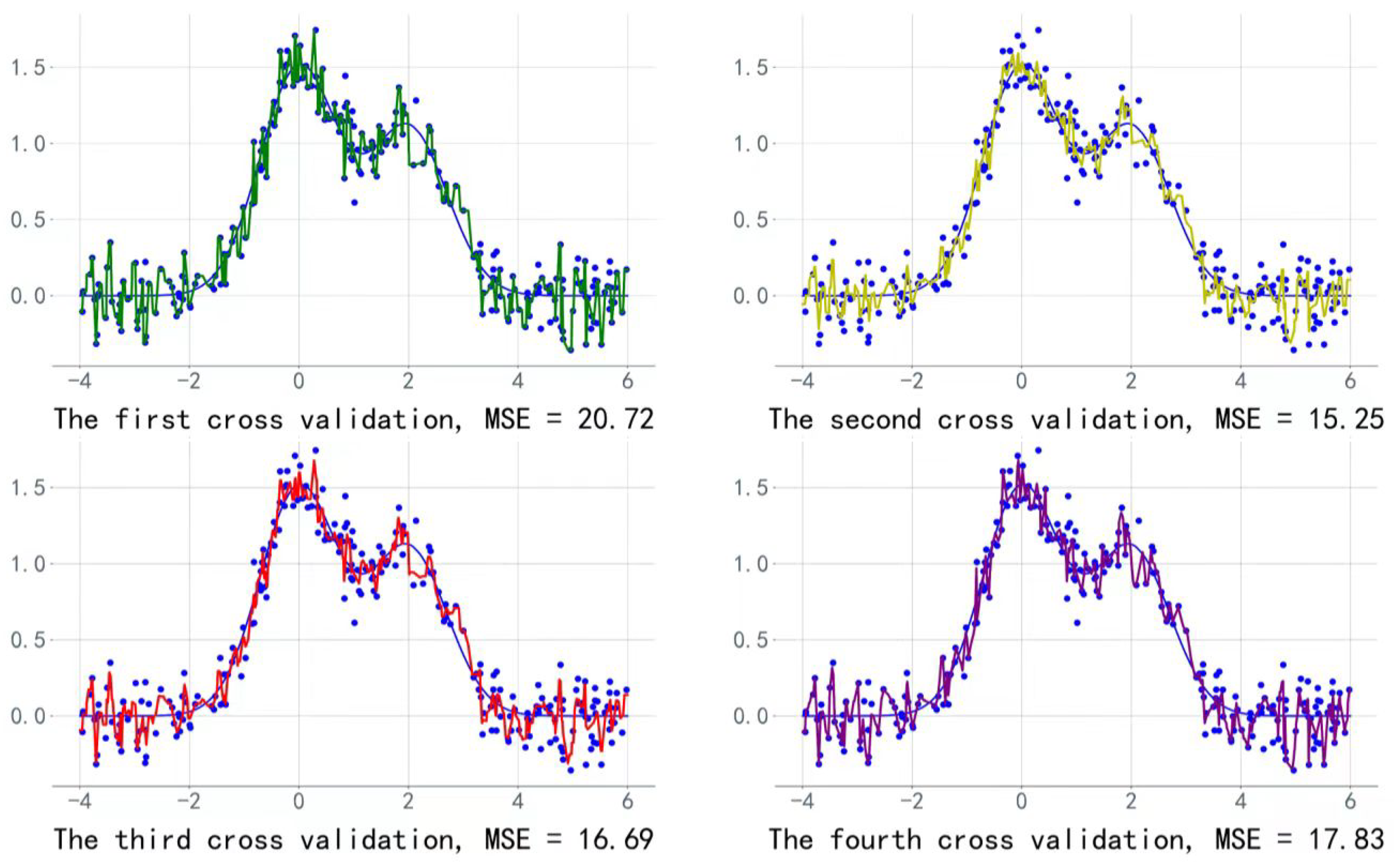
4.3.2. Establishing and Solving the LightGBM Sales Forecasting Model

LightGBM is an improved model based on decision tree and gradient boosting models that can be used for classification and regression problems. In addition, LightGBM has high accuracy in processing time-series-related data.

We set tweedie as the loss function in order to measure the degree of difference between the predicted values and the true values. Since the time series data existed in sequence and random partitions could lead to future data leakage, we adopted four-fold cross-validation instead of a random partition.

Using four-fold cross-validation required us to build the following four LGB models with the help of Python:

(1)

The training set used the data from the first 713 days and the validation set used the data from the 714-th day; early stop = 50 rounds;

(2)

The training set used the data from the first 714 days and the validation set used the data from the 715-th day; early stop = 50 rounds;

(3)

The training set used the data from the first 715 days and the validation set used the data from the 716-th day; early stop = 50 rounds;

(4)

The training set used the data from the first 716 days and the validation set used the data from the 717-th day; early stop = 50 rounds.

Calculations of the MSE metrics and visualization of the prediction effect of each round of cross-validation are shown in Figure 6.

We chose the LightGBM model with the smallest MSE value to predict the daily sales data of each vegetable category from 1 to 7 July 2023, as shown in

Table 5. LightGBM model forecast of the daily sales of each vegetable category in the following week.

Dates	Aquatic Rhizomes	Philodendron	Cauliflower (Brassica oleracea var. botrytis)	Eggplant	Capsicum	Edible Mushroom
1 July 2023	19.66	143.34	20.01	19.46	92.48	56.49
2 July 2023	21.82	131.05	24.49	29.69	88.75	55.61
3 July 2023	21.78	122.72	22.32	25.73	83.63	54.62
4 July 2023	25.10	112.13	26.64	28.91	76.74	53.47
5 July 2023	22.71	135.93	25.02	19.80	83.03	43.74
6 July 2023	26.69	118.42	28.44	26.72	81.63	51.71
7 July 2023	29.64	132.63	31.36	26.81	88.37	51.92

.

By combining the fitting expression with the daily sales volume and the daily average price of each vegetable category, we calculated the pricing strategy of the daily average price of each vegetable category from 1 to 7 July 2023, as shown in

Table 6. Forecast of the daily average prices of each vegetable category for the following week based on polynomial fitting.

Dates	Aquatic Rhizomes	Philodendron	Cauliflower (Brassica oleracea var. botrytis)	Eggplant	Capsicum	Edible Mushroom
1 July 2023	19.9	5.1	13.7	7.4	5.9	6.5
2 July 2023	19.0	5.2	15.2	7.5	5.7	5.5
3 July 2023	18.6	5.1	15.1	6.7	6.0	5.8
4 July 2023	18.5	5.7	15.2	6.4	6.5	5.9
5 July 2023	18.2	5.3	15.1	8.0	6.3	5.8
6 July 2023	17.1	5.2	13.2	7.8	6.3	5.5
7 July 2023	18.7	5.0	13.7	7.5	6.2	4.7

.

In summary, we established the LightGBM sales forecasting model to solve question two. Combined with previous sales data, we forecast the daily replenishment volume of each vegetable category for the following week. In addition, we developed a pricing strategy to maximize supermarket profits.

5. Solution to Question Three

5.1. Research Ideas

In this study, we constructed a model on the premise of meeting constraints and explored the optimal replenishment volume and pricing strategy to maximize supermarket revenue. Considering the large number of single items available for sale, the complex single-item sales attributes, and the various cumbersome constraints, we adopted the traditional dynamic programming model to solve the problem.

5.2. Preparation

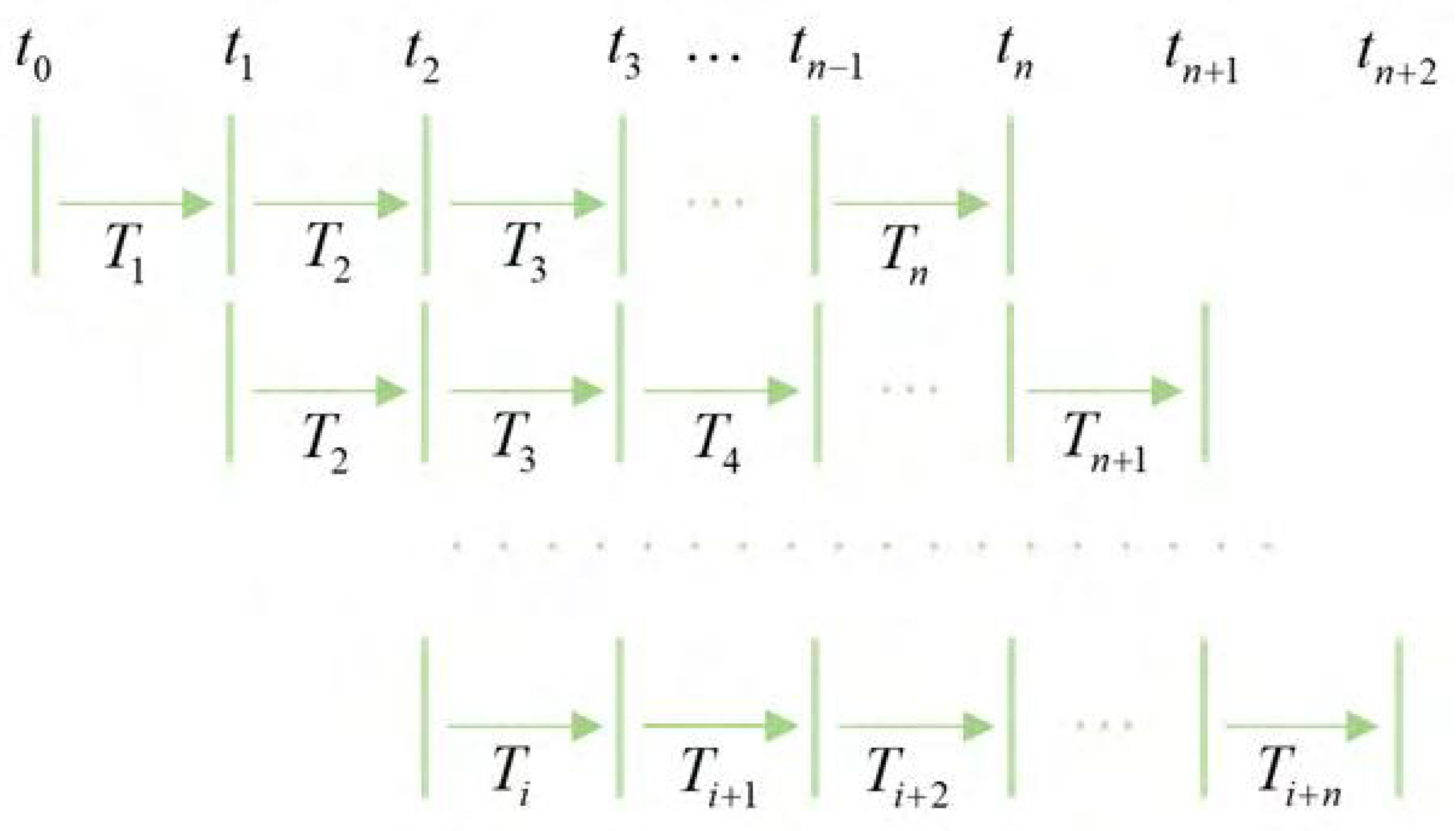
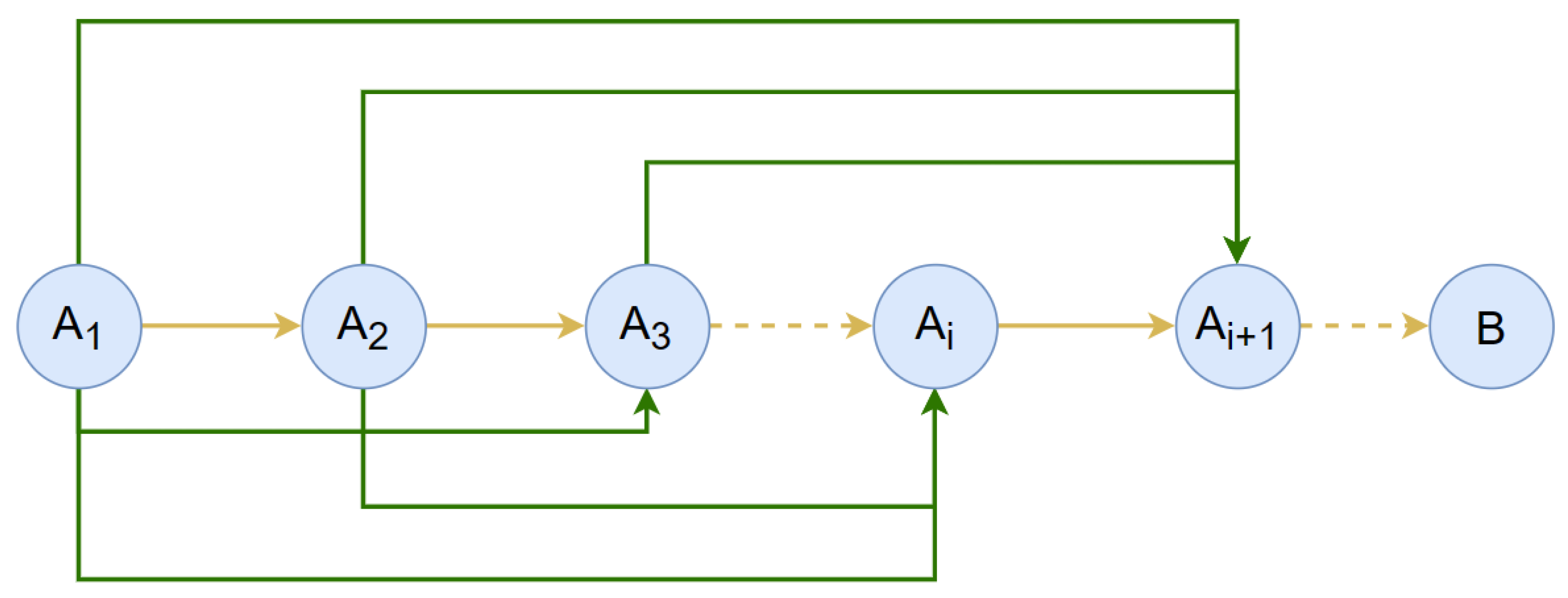
5.2.1. Preparation of the Dynamic Programming Sales Forecasting Model

Dynamic programming is the process of splitting a given problem into subproblems. The answers to the subproblems are inverted to arrive at a solution to the original problem. The principle of the dynamic programming model is to use mathematical induction to solve the surmised solution B based on the premise $A_n$ whose problem size is n. When the problem size is 0, it is known that inductive basis $A_0$ can derive B. For each integer i greater than or equal to 1, we assume that $A_i$ can derive B. Next, we add new conditions and information to $A_i$, and then we consider whether B can be deduced by $A_{i+1}$. The dynamic programming model principle is shown in Figure 7, where yellow arrows represent direct derivations, dashed arrows represent the omission of the procedure, and green arrows represent the processes that provide the conditions and information for direct derivations.

The core idea of dynamic programming is to achieve optimal allocation results according to constraints. The optimal value function is the optimal value of the indicator function, denoted as $f_k\left(s_k\right)$, which indicates the process from the beginning state in the $k-th$ stage to the termination state in the $n-th$ stage. The value of the indicator function is obtained by adopting the optimal strategy (generally, the maximum/minimum value), as follows:

$$f_k\left(s_k\right)=\underset{\left\{u_k,\cdots ,u_n\right\}}{opt}{V}_{k,n}\left(s_k,u_k,\cdots ,s_{n+1}\right).$$

In this study, firstly, we analyzed the actual supermarket sales and obtained the constraints, including the limit on the number of single products, the minimum purchase limit, the total purchase limit, and so on. Secondly, we processed the sales data from 24 to 30 June. Lastly, we analyzed the rationality and reliability of using these data.

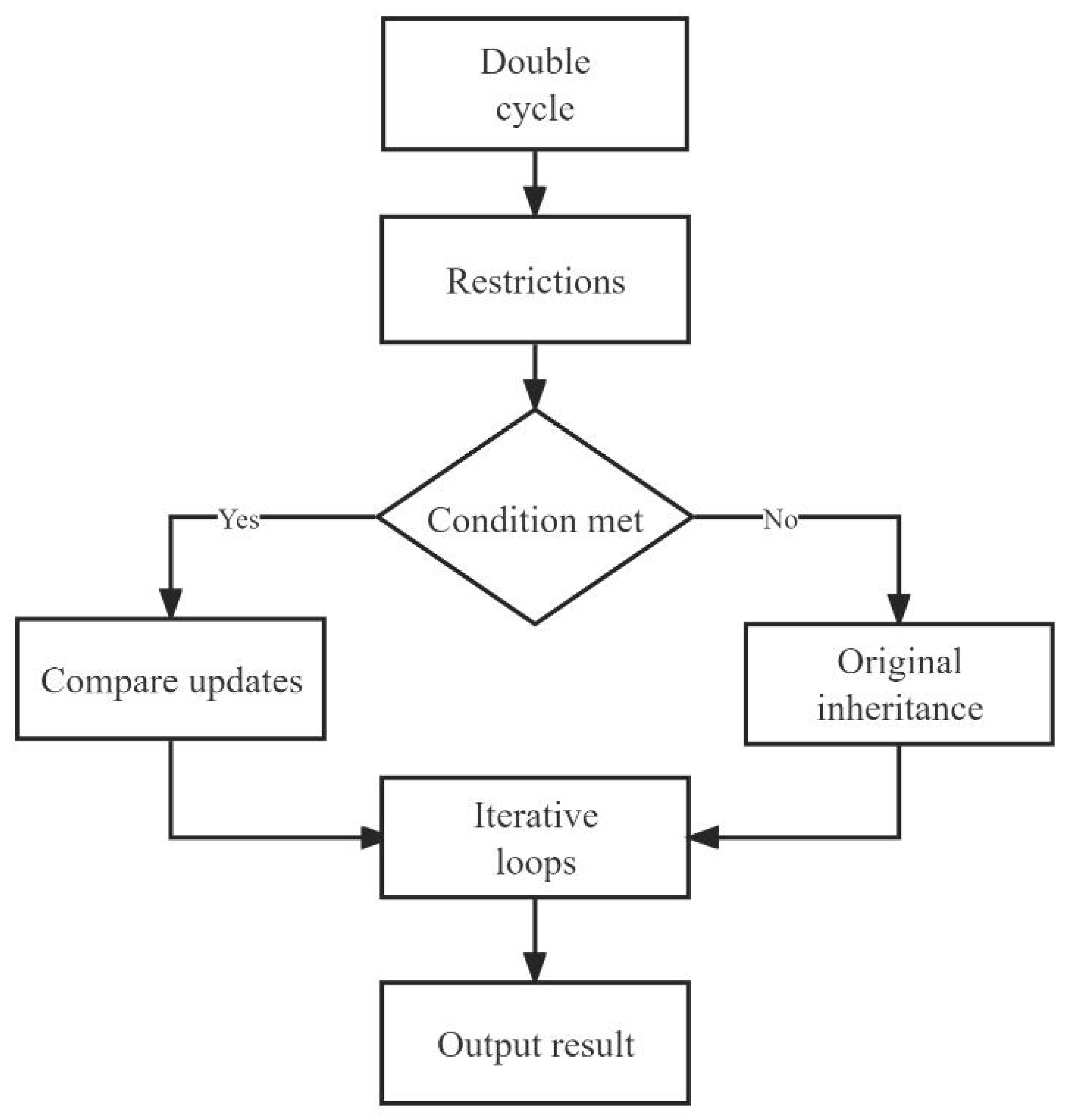
5.2.2. Modeling and Solving

Firstly, we decided upon the state and decision, which are key to dynamic programming. In the case of forecasting the sales of vegetable items, the state was “the number of items currently available for sale” and the decision was “whether to buy a new item” or “whether to increase/decrease the price of the item”.

Secondly, we defined the state transfer equation. The state transfer equation describes how a state variable transfers to another. In the $k-th$ stage, we already knew the value of the state variable. Then, once the decision variable was determined, we could determine the value of the state variable in the next stage. This correspondence can be expressed mathematically as

$$s_{k+1}=T_k(s_k,u_k),$$

where $s_{k+1}$ is the state variable in the k-th + 1 stage, $T_k$ is the state transfer function that describes the evolution of the state variables, $s_k$ is the state variable in the k-th stage, and $u_k$ is the decision variable in the k-th stage.

Finally, we defined the initial and boundary conditions, which are necessary for any dynamic programming problem. In this question, the initial condition was “the number and types of items available for sale on July 1” and the boundary conditions were “the purchase quantity of a single product shall not be less than 2.5 kg”, “the number of single products shall not exceed the upper limit”, and “the total purchase quantity shall not be higher than the upper limit”. The model traversed single items and weight ranges through two nested loops. The outer loop variable i represents the index of the single item and the inner loop variable j represents the current weight range. In each inner loop, the model performed a series of calculations and judgments. If the conditions were met, the model compared the value of whether or not to purchase the current individual item. If a greater value could be obtained by purchasing the current individual item, then the model updated the maximum value and the sequence of purchased items. Otherwise, the current item was not purchased. Our research ideas are shown in Figure 8.

After completing the iterative cycle, we obtained the maximum profit of USD $1239.86$. The single product sequence was the best purchase choice, as shown in

Table 7. Individual product replenishment volume and pricing table for July 1.

Single Vegetables	Replenishment (kg)	Sales Price (USD/kg)	Single Vegetables	Replenishment (kg)	Sales Price (USD/kg)
Shanghai Youth	3.86	4.12	Yunnan Oilseed Rape (Brassica campestris L.)	21.29	2.86
Yunnan Lettuce	2.92	5.73	Agaricus bisporus (Box)	10.00	3.40
Baby Chinese Cabbage (Mini-Sized Variety)	10.43	4.73	Small Wrinkled Skin (Portions)	11.29	1.54
Millet Peppers (Servings)	21.43	2.14	Baby Bok Choy	4.90	2.83
Snow Fungus (Tremella fuciformis)	5.93	3.21	Net Lotus Root	6.03	10.75
Honghu Lotus Roots	4.03	18.00	Seafood Mushroom (Pack)	8.86	1.95
Brussels Sprouts (Brassica oleracea var. botrytis)	13.30	2.32	Purple Eggplant (Solanum melongena L.)	10.90	3.75
Sweet Potato Tip	4.51	3.20	Wuhu Green Pepper	14.23	3.38
Amaranth Greens (Genus Amaranthus)	8.92	2.32	Spinach (Servings)	9.80	4.10
King Cobra or Chili (Naga Jolokia)	6.84	7.52	Screw Peppers (Servings)	11.29	3.28
Broccoli	12.56	7.82	Xixia Shiitake Mushroom	4.62	15.60
Golden Needle Mushroom (Box)	16.14	1.45	Long-Term Eggplant	4.21	6.98
Eggplant (Solanum melongena L.)	3.12	4.05	Cucumber	3.00	11.54
Zijiang Qingdian Scattered Flowers	6.30	9.36	Yunnan Lettuce (Servings)	32.29	3.60
Cabbage (Common in Chinese Medicine)	7.49	2.53	Fresh Fungus (Portions)	4.00	1.30
Ginger, Garlic, and  Millet Pepper Combo	7.00	2.44
Maximum Profit: USD 1239.86

.

In summary, we used Python to build a dynamic programming model to solve question three. We developed an optimal replenishment volume and pricing strategy, which let the supermarket maximize its income on the premise of meeting the constraints.

6. Conclusions

In this study, we addressed three questions. To answer the first question, we created pivot tables to analyze occupancy. We found that mosaic leaves, peppers, and edible mushrooms accounted for a larger proportion of the occupancy, while cauliflowers, aquatic rhizomes, and eggplants accounted for a smaller proportion. For single items, lettuce, cabbage, green pepper, screw pepper, enoki mushroom, and shiitake mushroom accounted for a large proportion of their respective categories. We used the Pearson correlation coefficient and the Mfuzz package based on fuzzy c-means (FCM) algorithm to analyze the correlation between vegetable categories and single products. We found that there was a strong correlation between vegetable categories. Moreover, the sales of vegetable items belonging to the same category exhibited the same patterns of change over time. In order to address the second question, we established the LightGBM sales forecasting model. Combined with previous sales data, we forecasted and planned an efficient daily replenishment volume for each vegetable category in the coming week. In addition, we developed a pricing strategy for vegetable categories to maximize supermarket profits. For the third question, we built a dynamic programming model combining an optimal replenishment volume with a product pricing strategy for single items that let the supermarket maximize its expected profits.

When constructing the dynamic programming model, we did not take into account whether the vegetable items were discounted or not. We conjecture that if we add a discount judgment to the model, we could be expected to solve some more complex and life-related problems, for example, how to develop replenishment plans and pricing strategies during holiday promotions.

References

1. Zhang, S.; Zhou, J. Analysis of factors and strategies affecting the efficiency of “agricultural super docking” of bulk vegetables. Shanxi Agric. Econ. 2023, 263–268. [Google Scholar] [CrossRef]
2. Li, G. Research on Price Formation and Stabilization Measures of the Whole Vegetable Industry Chain. Ph.D. Thesis, Nanjing University of Aeronautics and Astronautics, Nanjing, China, 2016. [Google Scholar]
3. Wei, D. Research on vegetable revenue insurance risk and pricing in Shandong. Rural Econ. Technol. 2021, 32, 69–70+160. [Google Scholar]
4. Zhu, R.; Fan, Z. Dynamic planning model and application of solution for merchandising. J. Shijiazhuang Econ. Coll. 2002, 3, 234–237. [Google Scholar] [CrossRef]
5. Yang, P.; Yin, X.; Zhang, G. Cluster analysis of fuzzy C-mean seismic attributes. Pet. Geophys. Explor. 2007, 42, 322–324+242+347+362. [Google Scholar]
6. Lu, Y. Research on Dynamic Pricing Problem of High Quality Fresh Vegetables in Supermarkets in China. Ph.D. Thesis, Beijing Jiaotong University, Beijing, China, 2010. [Google Scholar]
7. Yan, J.; Li, R. Research on resource allocation of health service stations based on state transfer equation. China Health Econ. 2012, 31, 61–64. [Google Scholar]
8. Wang, S. Research on the Formation Problem of Retail Price of Vegetables in Farmers’ Market. Ph.D. Thesis, Huazhong Agricultural University, Wuhan, China, 2014. [Google Scholar]
9. Song, J. Research on Optimization of Inventory Management of Vegetable Supply Chain in Shouguang City. Coop. Econ. Sci. Technol. 2015, 138–139. [Google Scholar] [CrossRef]
10. Wu, R. Application of state transfer equation in multi-stage decision-making evaluation of emergencies. Decis.-Mak. Explor. 2020, 7, 36–37. [Google Scholar]
11. Lu, M.; Zhang, W.; Xu, T. Optimizable replenishment strategy based on dynamic matrix model. Comput. Eng. Appl. 2021, 57, 263–268. [Google Scholar]
12. Feng, Z.; Zhang, H. A parameter estimation method for multivariate linear models based on residual vector l1-paradigm minimization with basis tracking. J. Hainan Norm. Univ. Nat. Sci. Ed. 2022, 35, 250–259+267. [Google Scholar]
13. Li, Y. Joint Replenishment and Pricing Collaborative Decision Making Considering Investment in Preservation Technology. Ph.D. Thesis, Chongqing Jiaotong University, Chongqing, China, 2023. [Google Scholar]
14. Xie, J.; Zhang, H.; Li, D.; Yu, X.; Deng, J. Optimized deep forest algorithm based on Lightgbm and XGBoost. J. Nanjing Univ. Nat. Sci. 2023, 59, 833–840. [Google Scholar] [CrossRef]
15. Xu, X.; Zhang, Y.; Fang, Y.; Liu, S. Research on Inventory Management Optimization of A Trading Company Based on k-means Clustering Algorithm. China Storage Transp. 2024, 143–144. [Google Scholar] [CrossRef]
16. Guo, L.; Guo, Z.; Jia, H.; Fan, R. Identification of residential electricity theft based on Pearson correlation coefficient and SVM. J. Hebei Univ. Nat. Sci. Ed. 2023, 43, 357–363. [Google Scholar]
17. Liu, H. Research and application of network intrusion detection method based on deep learning. Comput. Program. Ski. Maint. 2023, 162–165. [Google Scholar] [CrossRef]
Figure 1. Sales’ outliers box plot test.
Axioms 13 00257 g001
Figure 2. Profitability outliers box plot test.
Axioms 13 00257 g002
Figure 3. Sliding time window null processing diagram.
Axioms 13 00257 g003
Figure 4. Flowchart of solution to question one.
Axioms 13 00257 g004
Figure 5. Vegetable item clustering visualization results plot.
Axioms 13 00257 g005
Figure 6. Visualization of the fitting effect of each round of cross-validation.
Axioms 13 00257 g006
Figure 7. Schematic diagram of dynamic programming.
Axioms 13 00257 g007
Figure 8. Flowchart of solution to question three.
Axioms 13 00257 g008