

Distributed Charging Strategy of PEVs in SCS with Feeder Constraints Based on Generalized Nash Equilibria


Abstract
:1. Introduction
1.1. Background and Research Gaps
1.2. Motivation
1.3. Contributions
- (1)
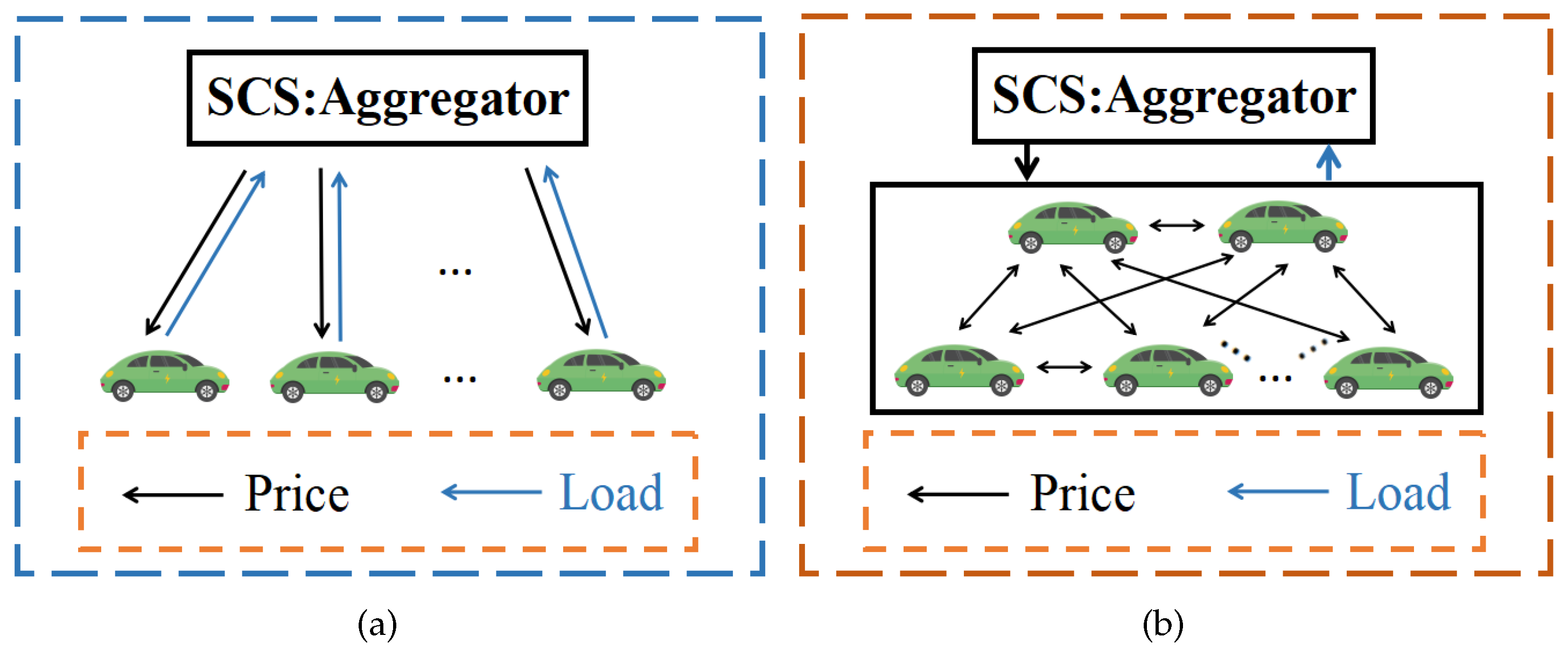
- To take into account the flexible property of PEVs to a greater extent; unlike the interactions considered by the V2G mechanism [20], we employ a novel interaction mechanism between PEVs and SCS, which integrates the V2V mechanism to allow the interaction between PEVs. At the same time, in order to reduce the duration of the total SCS load peak and minimize the cost to the PEV owner, we develop a non-cooperative game framework that considers distribution feeder overload constraints and propose a novel price-driven charging control game that considers both minimizing charging costs and reducing feeder overload and avoids grid collapse.
- (2)
- To solve the generalized Nash equilibria problem (GNEP) considered in this article, we employ a distributed algorithm based on forward–backward operator splitting methods [30,31,32]. Using this algorithm, we can simultaneously treat the inequality constraints and the equality constraints in GNEP. We put together the constraints of all PEVs in GNEP from a global perspective, putting the local constraints into the global coupling constraints, and then treating the inequality constraints in GNEP together. Simulation results verify the effectiveness of the algorithm.
2. System Model and Problem Formulation
2.1. System Model
2.2. Problem Formulation
3. Non-Cooperative PEV Charging Game
3.1. Game Model
3.2. Existence of GNE
4. Distributed Algorithm
4.1. Target Question
4.2. Constraint Handling
4.3. Element Derivation
4.4. Distributed Algorithm
| Algorithm 1 Distributed Algorithm Based on Forward-Backward Operator Splitting Methods |
|
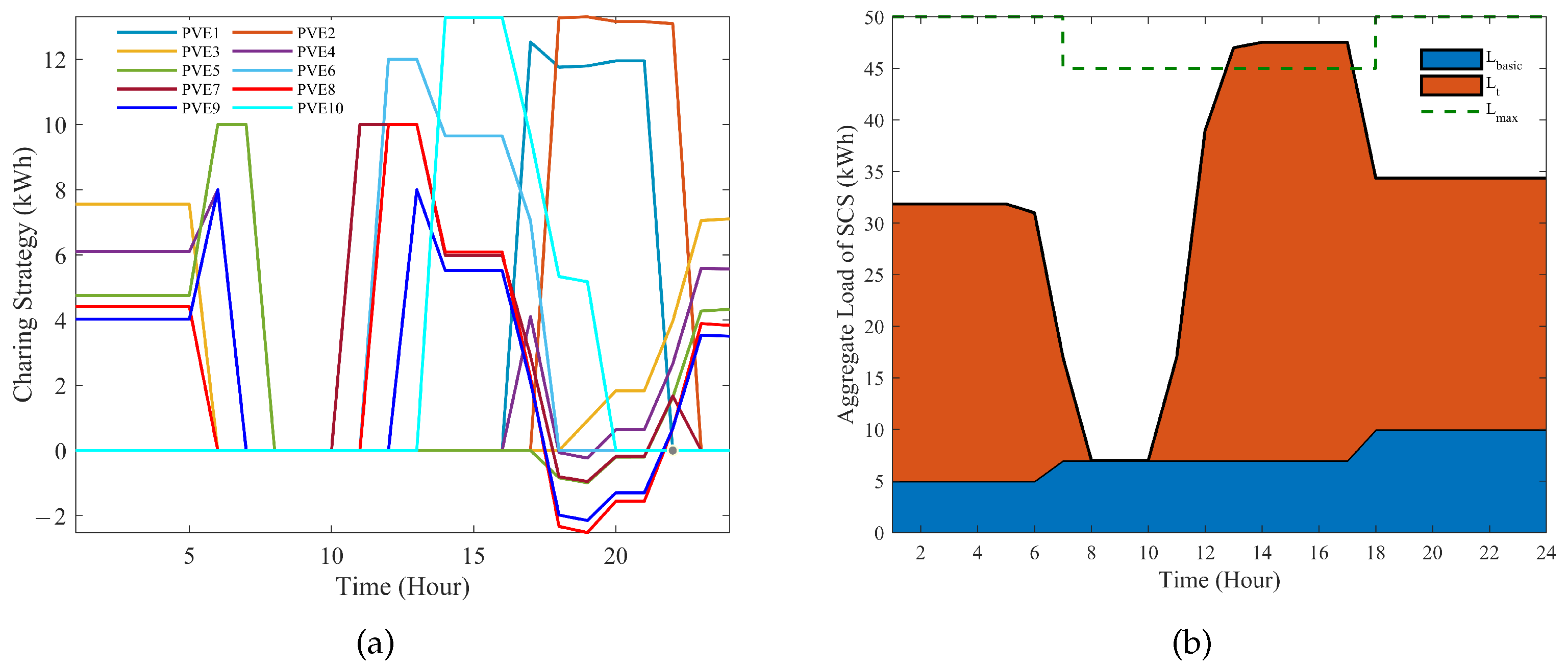
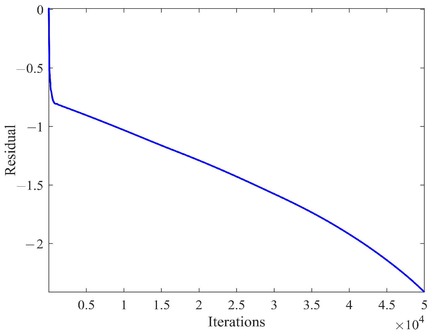
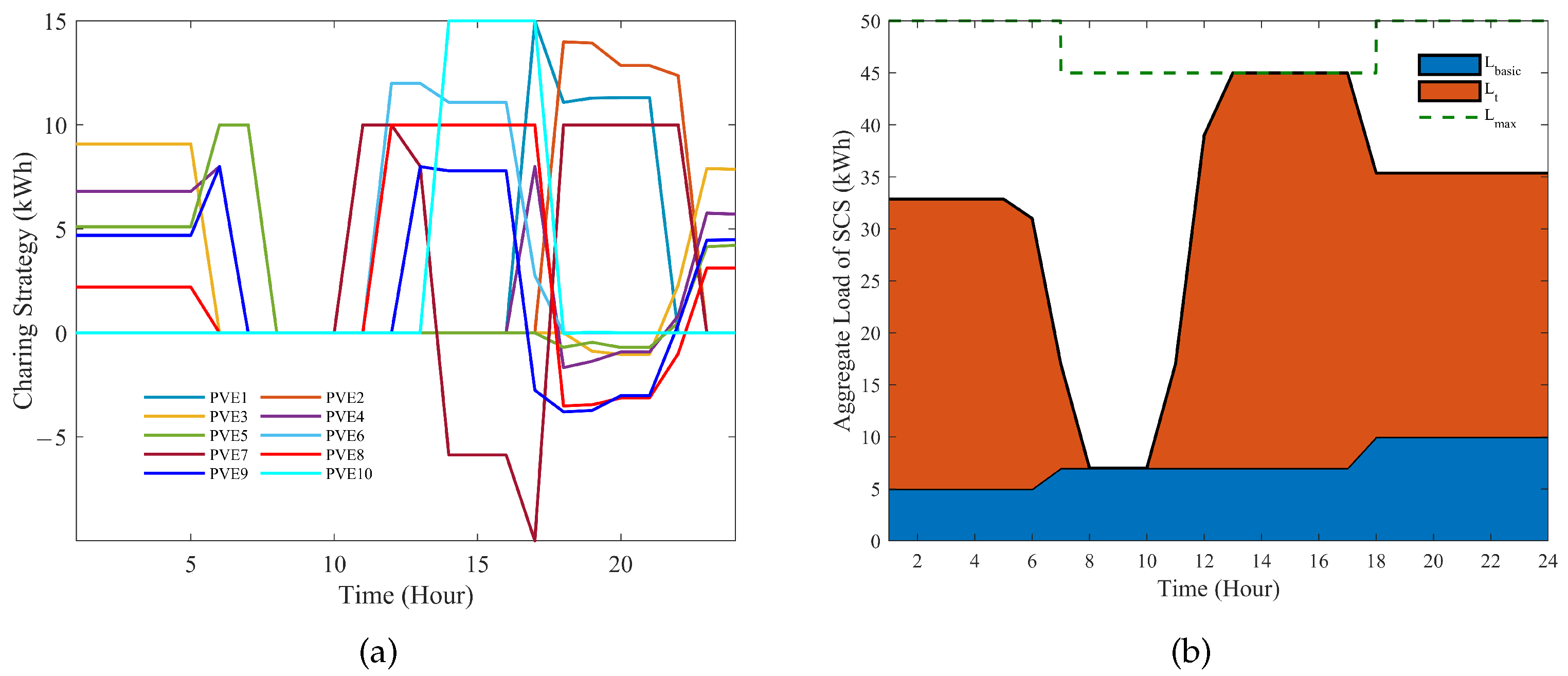
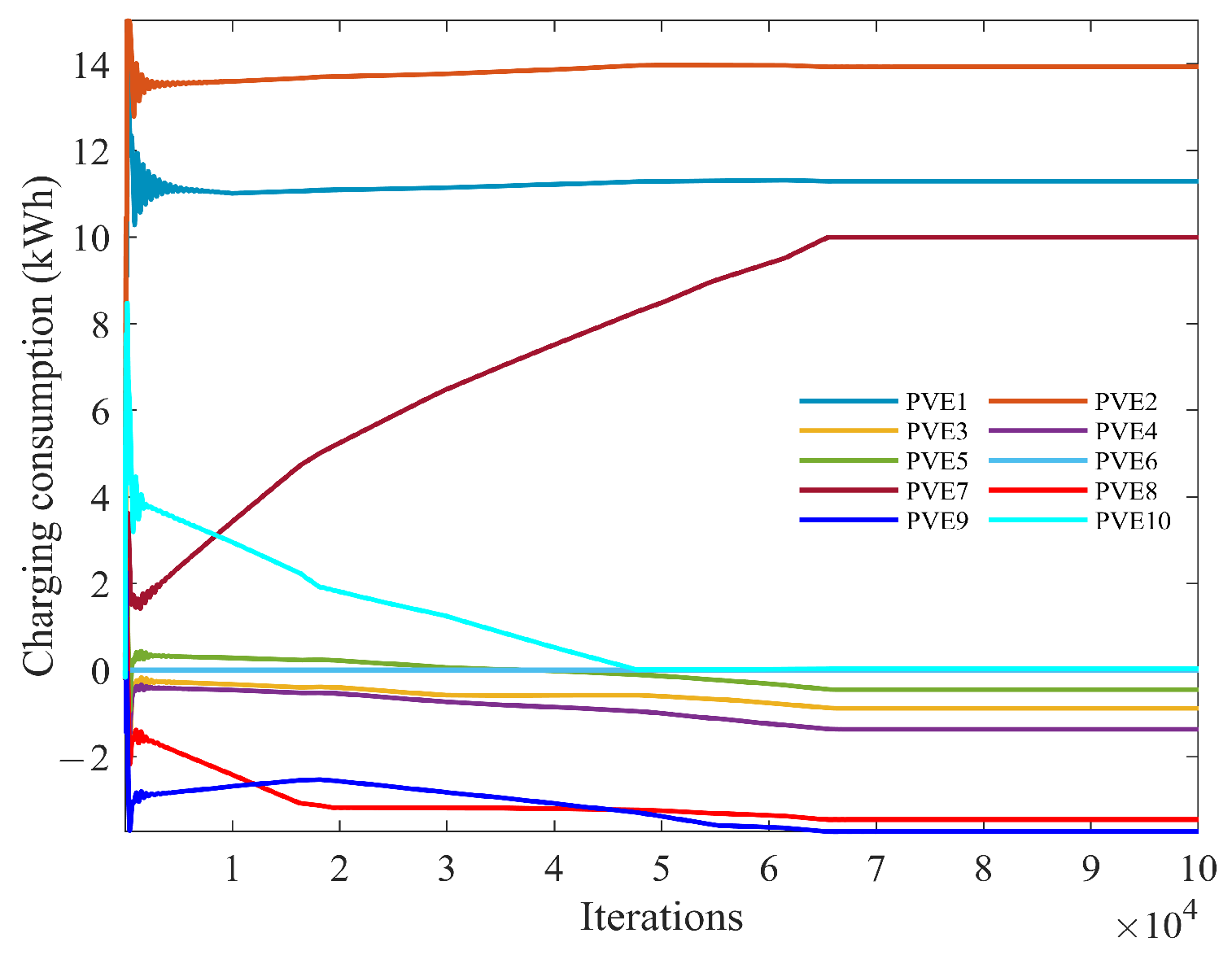
5. Simulation Results
6. Conclusions
Author Contributions
Funding
Data Availability Statement
Conflicts of Interest
Nomenclature
| Set of all PEVs | |
| Set of charging time periods | |
| Set of distribution feeders | |
| Charging power of PEV n at time t | |
| Charging curve of PEV n (PEVs) over the entire charging horizon | |
| Required energy of PEV n | |
| Initial/Terminal energy level of PEV n | |
| Lower/Upper battery capacity limit of PEV n | |
| Energy level of PEV n at time t | |
| Rated charging/discharging power of PEV n | |
| Total load of PEVs on feeder l at time t | |
| Overload control threshold on feeder l at time t | |
| Maximum PEV demand that feeder l can support at time t | |
| Maximum loading capacity of feeder l at time t | |
| Basic demand load (i.e., non-PEV demand) transmitted on feeder l at time t (over the entire charging horizon) | |
| Set of distribution feeders that transfer power from the distribution substation to PEV n | |
| Set of PEVs using the distribution feeder l to carry the power | |
| Set of feasible charging configurations for PEV n (PEVs) | |
| Electricity price at time t | |
| Positive price coefficients at time | |
| Aggregate load of SCS at time t | |
| Energy cost of SCS at time t | |
| Total energy cost of SCS | |
| Fees paid by PEV n | |
| Index of profitability | |
| Proportion of the total energy consumption of PEV n in the aggregate load of SCS | |
| Cost function of PEV n | |
| Charging strategies of all PEVs except PEV n | |
| Generalized Nash equilibria of G | |
| Local data of PEV n (PEVs) | |
| One vector of T dimension | |
| Transpose of A | |
| Pseudo gradient for cost function of PEV n | |
| Column vector of pseudo gradient for cost function of PEVs | |
| Inequality constraint factors of PEV n (PEVs) | |
| Equality constraint factors of PEV n (PEVs) | |
| Dual variables of PEV n (PEVs) | |
| Zero vector (matrix) of n () dimension | |
| Set of neighbors of PEV n | |
| Local copy of multiplier of PEV n | |
| Local auxiliary variable of PEV n | |
| k | Index of iterations |
| M | Dimension of local data for PEV n |
| Euclidean space of M dimension (non-negative) | |
| Fixed constant step-sizes of PEV n |
References
- You, Y.; Yi, L. Energy industry Carbon neutrality transition path: Corpus-based AHP-DEMATEL system modelling. Energy Rep. 2022, 8, 25–39. [Google Scholar] [CrossRef]
- Esmaili, M.; Goldoust, A. Multi-objective optimal charging of plug-in electric vehicles in unbalanced distribution networks. Int. J. Electr. Power Energy Syst. 2015, 73, 644–652. [Google Scholar] [CrossRef]
- Jiang, H.; Ning, S.; Ge, Q. Multi-objective optimal dispatching of microgrid with large-scale electric vehicles. IEEE Access 2019, 7, 145880–145888. [Google Scholar] [CrossRef]
- Rahbari-Asr, N.; Chow, M.Y. Cooperative distributed demand management for community charging of PHEV/PEVs based on KKT conditions and consensus networks. IEEE Trans. Ind. Inform. 2014, 10, 1907–1916. [Google Scholar] [CrossRef]
- You, P.; Yang, Z.; Chow, M.Y.; Sun, Y. Optimal cooperative charging strategy for a smart charging station of electric vehicles. IEEE Trans. Power Syst. 2015, 31, 2946–2956. [Google Scholar] [CrossRef]
- Tan, K.M.; Ramachandaramurthy, V.K.; Yong, J.Y. Integration of electric vehicles in smart grid: A review on vehicle to grid technologies and optimization techniques. Renew. Sustain. Energy Rev. 2016, 53, 720–732. [Google Scholar] [CrossRef]
- Berthold, F.; Ravey, A.; Blunier, B.; Bouquain, D.; Williamson, S.; Miraoui, A. Design and development of a smart control strategy for plug-in hybrid vehicles including vehicle-to-home functionality. IEEE Trans. Transp. Electrif. 2015, 1, 168–177. [Google Scholar] [CrossRef]
- Nguyen, D.T.; Le, L.B. Joint optimization of electric vehicle and home energy scheduling considering user comfort preference. IEEE Trans. Smart Grid 2013, 5, 188–199. [Google Scholar] [CrossRef]
- Tuballa, M.L.; Abundo, M.L. A review of the development of Smart Grid technologies. Renew. Sustain. Energy Rev. 2016, 59, 710–725. [Google Scholar] [CrossRef]
- Goli, P.; Shireen, W. PV powered smart charging station for PHEVs. Renew. Energy 2014, 66, 280–287. [Google Scholar] [CrossRef]
- Wan, Y.; Qin, J.; Li, F.; Yu, X.; Kang, Y. Game theoretic-based distributed charging strategy for PEVs in a smart charging station. IEEE Trans. Smart Grid 2020, 12, 538–547. [Google Scholar] [CrossRef]
- Zhang, H.; Moura, S.J.; Hu, Z.; Qi, W.; Song, Y. A second-order cone programming model for planning PEV fast-charging stations. IEEE Trans. Power Syst. 2017, 33, 2763–2777. [Google Scholar] [CrossRef]
- Tan, J.; Wang, L. Integration of plug-in hybrid electric vehicles into residential distribution grid based on two-layer intelligent optimization. IEEE Trans. Smart Grid 2014, 5, 1774–1784. [Google Scholar] [CrossRef]
- Hagh, M.T.; Gargari, M.Z.; Pakdel, M.J.V. Sequential analysis of optimal transmission switching with contingency assessment. IET Gener. Transm. Distrib. 2018, 12, 1390–1396. [Google Scholar] [CrossRef]
- Bai, X.; Qiao, W.; Wei, H.; Huang, F.; Chen, Y. Bidirectional coordinating dispatch of large-scale V2G in a future smart grid using complementarity optimization. Int. J. Electr. Power Energy Syst. 2015, 68, 269–277. [Google Scholar] [CrossRef]
- Sun, S.; Yang, Q.; Yan, W. Optimal temporal-spatial electric vehicle charging demand scheduling considering transportation-power grid couplings. In Proceedings of the 2018 IEEE Power & Energy Society General Meeting (PESGM), Portland, OR, USA, 5–10 August 2018; pp. 1–5. [Google Scholar]
- Cheng, P.H.; Huang, T.H.; Chien, Y.W.; Wu, C.L.; Tai, C.S.; Fu, L.C. Demand-side management in residential community realizing sharing economy with bidirectional PEV while additionally considering commercial area. Int. J. Electr. Power Energy Syst. 2020, 116, 105512. [Google Scholar] [CrossRef]
- Wang, L.; Chen, B. Distributed control for large-scale plug-in electric vehicle charging with a consensus algorithm. Int. J. Electr. Power Energy Syst. 2019, 109, 369–383. [Google Scholar] [CrossRef]
- Lee, M. Multi-Task Deep Learning Games: Investigating Nash Equilibria and Convergence Properties. Axioms 2023, 12, 569. [Google Scholar] [CrossRef]
- Tushar, W.; Saad, W.; Poor, H.V.; Smith, D.B. Economics of electric vehicle charging: A game theoretic approach. IEEE Trans. Smart Grid 2012, 3, 1767–1778. [Google Scholar] [CrossRef]
- Yang, X.; Wang, G.; He, H.; Lu, J.; Zhang, Y. Automated demand response framework in ELNs: Decentralized scheduling and smart contract. IEEE Trans. Syst. Man Cybern. Syst. 2019, 50, 58–72. [Google Scholar] [CrossRef]
- Li, J.; Li, C.; Xu, Y.; Dong, Z.Y.; Wong, K.P.; Huang, T. Noncooperative game-based distributed charging control for plug-in electric vehicles in distribution networks. IEEE Trans. Ind. Inform. 2016, 14, 301–310. [Google Scholar] [CrossRef]
- Li, C.; Liu, C.; Deng, K.; Yu, X.; Huang, T. Data-driven charging strategy of PEVs under transformer aging risk. IEEE Trans. Control Syst. Technol. 2017, 26, 1386–1399. [Google Scholar] [CrossRef]
- Alsabbagh, A.; Yin, H.; Ma, C. Distributed electric vehicles charging management with social contribution concept. IEEE Trans. Ind. Inform. 2019, 16, 3483–3492. [Google Scholar] [CrossRef]
- Iria, J.; Coelho, A.; Soares, F. Network-secure bidding strategy for aggregators under uncertainty. Sustain. Energy Grids Netw. 2022, 30, 100666. [Google Scholar] [CrossRef]
- Ghavami, A.; Kar, K.; Gupta, A. Decentralized charging of plug-in electric vehicles with distribution feeder overload control. IEEE Trans. Autom. Control 2016, 61, 3527–3532. [Google Scholar] [CrossRef]
- Ardakanian, O.; Keshav, S.; Rosenberg, C. Real-time distributed control for smart electric vehicle chargers: From a static to a dynamic study. IEEE Trans. Smart Grid 2014, 5, 2295–2305. [Google Scholar] [CrossRef]
- Harks, T.; Schwarz, J. Generalized Nash equilibrium problems with mixed-integer variables. Math. Program. 2024, 2024, 1–47. [Google Scholar] [CrossRef]
- Drăgan, V.; Ivanov, I.G.; Popa, I.L. A Game—Theoretic Model for a Stochastic Linear Quadratic Tracking Problem. Axioms 2023, 12, 76. [Google Scholar] [CrossRef]
- Yi, P.; Pavel, L. An operator splitting approach for distributed generalized Nash equilibria computation. Automatica 2019, 102, 111–121. [Google Scholar] [CrossRef]
- Izuchukwu, C.; Reich, S.; Shehu, Y.; Taiwo, A. Strong convergence of forward–reflected–backward splitting methods for solving monotone inclusions with applications to image restoration and optimal control. J. Sci. Comput. 2023, 94, 73. [Google Scholar] [CrossRef]
- Dadashi, V.; Postolache, M. Forward–backward splitting algorithm for fixed point problems and zeros of the sum of monotone operators. Arab. J. Math. 2020, 9, 89–99. [Google Scholar] [CrossRef]
- Lin, X.; Zhang, T.; Li, M.; Zhang, R.; Zhang, W. Multi-Player Non-Cooperative Game Strategy of a Nonlinear Stochastic System with Time-Varying Parameters. Axioms 2023, 13, 3. [Google Scholar] [CrossRef]
- Wang, Z.; Li, X.; Liang, W.; Ma, J. Does a New Electric Vehicle Manufacturer Have the Incentive for Battery Life Investment? A Study Based on the Game Framework. Mathematics 2023, 11, 3551. [Google Scholar] [CrossRef]
- Yang, L.; Li, X.; Sun, M.; Sun, C. Hybrid policy-based reinforcement learning of adaptive energy management for the Energy transmission-constrained island group. IEEE Trans. Ind. Inform. 2023. [Google Scholar] [CrossRef]
- Li, Y.; Zhang, H.; Liang, X.; Huang, B. Event-triggered-based distributed cooperative energy management for multienergy systems. IEEE Trans. Ind. Inform. 2018, 15, 2008–2022. [Google Scholar] [CrossRef]


| PEV | AT | DT | |||||
|---|---|---|---|---|---|---|---|
| 1 | 7.5 | 67.5 | 5 | 75 | 15 | 17:00 | 22:00 |
| 2 | 6 | 72 | 5 | 80 | 15 | 18:00 | 23:00 |
| 3 | 7 | 67.5 | 5 | 75 | 10 | 19:00 | 6:00 |
| 4 | 5.6 | 63 | 5 | 70 | 8 | 17:00 | 7:00 |
| 5 | 6.7 | 58.5 | 5 | 65 | 10 | 11:00 | 23:00 |
| 6 | 7.5 | 67.5 | 5 | 75 | 12 | 12:00 | 18:00 |
| 7 | 8.1 | 58.5 | 5 | 65 | 10 | 11:00 | 23:00 |
| 8 | 9 | 72 | 5 | 80 | 10 | 12:00 | 6:00 |
| 9 | 7.2 | 63 | 5 | 70 | 8 | 13:00 | 7:00 |
| 10 | 7.5 | 67.5 | 5 | 75 | 15 | 14:00 | 20:00 |
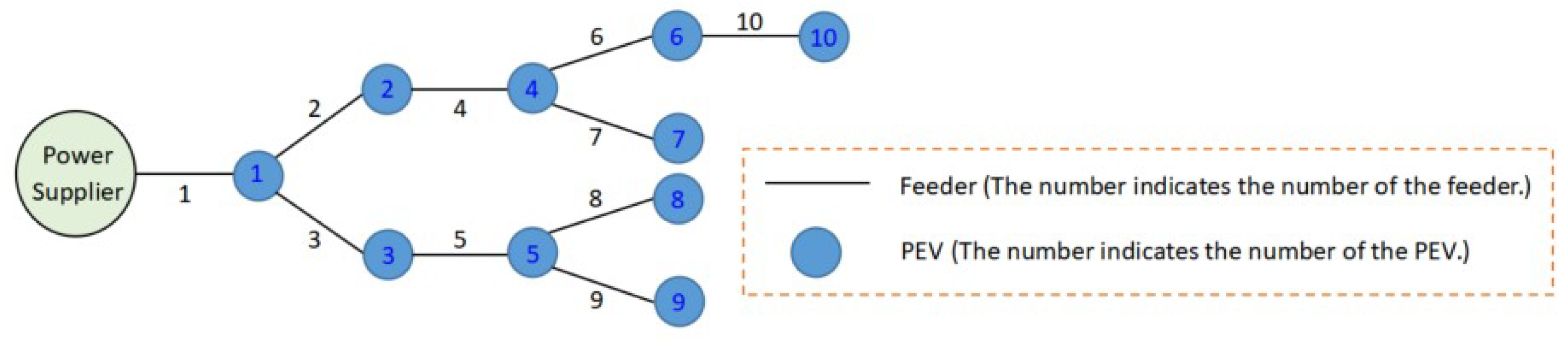
| Feeder | Affected PEVs (Remaining at 0) |
|---|---|
| 1 | 1, 2, 3, 4, 5, 6, 7, 8, 9, 10 |
| 2 | 2, 4, 6, 7, 10, 0, 0, 0, 0, 0 |
| 3 | 3, 5, 8, 9, 0, 0, 0, 0, 0, 0 |
| 4 | 4, 6, 7, 10, 0, 0, 0, 0, 0, 0 |
| 5 | 5, 8, 9, 0, 0, 0, 0, 0, 0, 0 |
| 6 | 6, 10, 0, 0, 0, 0, 0, 0, 0, 0 |
| 7 | 7, 0, 0, 0, 0, 0, 0, 0, 0, 0 |
| 8 | 8, 0, 0, 0, 0, 0, 0, 0, 0, 0 |
| 9 | 9, 0, 0, 0, 0, 0, 0, 0, 0, 0 |
| 10 | 10, 0, 0, 0, 0, 0, 0, 0, 0, 0 |
| Feeder | 1:00–6:00 | 7:00–17:00 | 18:00–24:00 |
|---|---|---|---|
| 1 | 50 | 45 | 50 |
| 2 | 48 | 44.5 | 47 |
| 3 | 46 | 44 | 44 |
| 4 | 44 | 43.5 | 41 |
| 5 | 42 | 43 | 38 |
| 6 | 40 | 42.5 | 35 |
| 7 | 38 | 42 | 32 |
| 8 | 36 | 41.5 | 29 |
| 9 | 34 | 41 | 26 |
| 10 | 32 | 40.5 | 23 |
| Feeder | 1:00–6:00 | 7:00–17:00 | 18:00–24:00 |
|---|---|---|---|
| 1 | 5 | 7 | 10 |
| 2 | 4.8 | 6.9 | 9 |
| 3 | 4.6 | 6.8 | 8.1 |
| 4 | 4.4 | 6.7 | 7.3 |
| 5 | 4.2 | 6.6 | 6.6 |
| 6 | 4 | 6.5 | 6 |
| 7 | 3.8 | 6.4 | 5.5 |
| 8 | 3.6 | 6.3 | 5.1 |
| 9 | 3.4 | 6.2 | 4.8 |
| 10 | 3.2 | 6.1 | 4.6 |
Disclaimer/Publisher’s Note: The statements, opinions and data contained in all publications are solely those of the individual author(s) and contributor(s) and not of MDPI and/or the editor(s). MDPI and/or the editor(s) disclaim responsibility for any injury to people or property resulting from any ideas, methods, instructions or products referred to in the content. |
© 2024 by the authors. Licensee MDPI, Basel, Switzerland. This article is an open access article distributed under the terms and conditions of the Creative Commons Attribution (CC BY) license (https://creativecommons.org/licenses/by/4.0/).
Share and Cite
Tang, J.; Li, H.; Chen, M.; Shi, Y.; Zheng, L.; Wang, H. Distributed Charging Strategy of PEVs in SCS with Feeder Constraints Based on Generalized Nash Equilibria. Axioms 2024, 13, 259. https://doi.org/10.3390/axioms13040259
Tang J, Li H, Chen M, Shi Y, Zheng L, Wang H. Distributed Charging Strategy of PEVs in SCS with Feeder Constraints Based on Generalized Nash Equilibria. Axioms. 2024; 13(4):259. https://doi.org/10.3390/axioms13040259
Chicago/Turabian StyleTang, Jialong, Huaqing Li, Menggang Chen, Yawei Shi, Lifeng Zheng, and Huiwei Wang. 2024. "Distributed Charging Strategy of PEVs in SCS with Feeder Constraints Based on Generalized Nash Equilibria" Axioms 13, no. 4: 259. https://doi.org/10.3390/axioms13040259