Hermite–Hadamard–Mercer-Type Inequalities for Three-Times Differentiable Functions

Abstract

In this study, an integral identity is given in order to present some Hermite–Hadamard–Mercer-type inequalities for functions whose powers of the absolute values of the third derivatives are convex. Several consequences and three applications to special means are given, as well as four examples with graphics which illustrate the validity of the results. Moreover, several Hermite–Hadamard–Mercer-type inequalities for fractional integrals for functions whose powers of the absolute values of the third derivatives are convex are presented.

1. Introduction

Convex analysis, as a branch of mathematical analysis, has an important role in mathematics, numerical analysis, optimization theory, convex programming and statistics, with convex functions being very important in the literature. Applications of mathematical inequalities play significant roles in mathematics, special functions, physics, fractals, number theory, and many other fields. So is not surprising that this subject has generated considerable interest for many mathematicians, being a very useful instrument in the recent development of different branches of mathematics. The classical inequality of Hermite–Hadamard was extended and generalized in many directions in the last decade, due to its quality among mathematical inequalities. This inequality has been studied by many scholars, for example, [1,2,3,4,5,6,7,8,9,10,11,12,13,14,15], and references therein. From the study of the Hermite–Hadamard inequality the Ostrowski, Simpson, midpoint, and trapezoidal inequalities were also obtained, as well as many Hermite–Hadamard-like inequalities [16,17]. Some studies on Hermite–Hadamard-like inequalities for functions whose third derivatives in absolute value are convex can also be found in [18,19,20].

We begin by recalling below the classical definition for convex functions; see [7].

Definition 1 

([7]). A function $h:I\subset \mathbb{R}\to \mathbb{R}$ is said to be convex on the interval I if we have

$$h(tx+(1-t\left)y\right)\le th\left(x\right)+(1-t)h\left(y\right)$$

(1)

for all $x,y\in I$, and $t\in [0,1].$ The function h is said to be concave on I if the inequality (1) is satisfied in the reverse direction.

The classical Hermite–Hadamard inequality for convex functions, known from the literature, see [21], is “

$$h\left(\frac{b+c}{2}\right)\le \frac{1}{c-b}{\int }_b^{c}h\left(x\right)dx\le \frac{h\left(b\right)+h\left(c\right)}{2},$$

(2)

with $h:[b,c]\to \mathbb{R}$ being the convex function. Moreover, if the function h is concave, then the inequality (2) holds in the reverse direction”. This inequality was introduced by C. Hermite in [22] and studied by J. Hadamard in [21].

An interesting form of Jensen’s inequality, which was given in 2003 by Mercer in [23], is stated below. This inequality is known as the Jensen–Mercer inequality.

Theorem 1 

([23]). For a convex mapping $h:[b,c]\to \mathbb{R}$, the subsequent inequality is valid for all values of ${\omega }_j\in [b,c](j=1,\dots ,n)$:

$$h(b+c-\sum _{j=1}^n{u}_j{\omega }_j)\le h\left(b\right)+h\left(c\right)-\sum _{j=1}^n{u}_{j}h\left({\omega }_j\right),$$

(3)

where $u_j\in [0,1](j=1,\dots ,n)$ and ${\sum }_{j=1}^n{u}_j=1.$

The Jensen–Mercer inequality is important also in information theory; see Khan et al. [24], where they presented new estimates for Csiszar divergence and Zipf–Mandelbrot entropy.

A refinement of the Hermite–Hadamard inequality was presented by using a previous inequality in [25]:

Theorem 2. 

For a convex mapping $h:[b,c]\to \mathbb{R}$, the subsequent inequalities are valid for every value of $\omega ,\mu \in [b,c]$ and $\omega <\mu$:

$$h(b+c-\frac{\omega +\mu }{2})\le h\left(b\right)+h\left(c\right)-\frac{1}{\mu -\omega }{\int }_{\omega }^{\mu }h\left(u\right)du\le h\left(b\right)+h\left(c\right)-h(\frac{\omega +\mu }{2})$$

(4)

and

$$h(b+c-\frac{\omega +\mu }{2})\le \frac{1}{\mu -\omega }{\int }_{b+c-\mu }^{b+c-\omega }h\left(u\right)du$$

(5)

$$\le \frac{h(b+c-\omega )+h(b+c-\mu )}{2}$$

$$\le h\left(b\right)+h\left(c\right)-\frac{h\left(\omega \right)+h\left(\mu \right)}{2}.$$

If $b=\omega$ and $c=\mu$ are chosen in (5), then we have the classical Hermite–Hadamard inequality.

The Hermite–Hadamard–Mercer inequalities have been improved and generalized in many directions in recent years by many researchers; see, for example, [26,27,28,29,30,31,32]. Thus, in [26,27] new variants of Hermite–Hadamard–Mercer inequalities are established for Riemann–Liouville fractional integrals, and in [28,29] Hermite–Hadamard–Mercer-type inequalities for generalized fractional integrals and for fractional integrals and differentiable functions are proven. New estimate bounds are given for Ostrowski-type inequalities by using the Jensen–Mercer inequality in [30] and the concept of convexity for interval-valued functions was used to find fractional Hermite–Hadamard–Mercer-type inequalities in [31]. In addition, several Hermite–Hadamard–Mercer-type inequalities were presented for harmonically convex functions in [32].

It is necessary for our goal to recall the following three Hermite–Hadamard–Mercer-type inequalities established in [33] for twice-differentiable and convex functions.

Theorem 3 

([33]). If the conditions of lemma 1 from [33] hold for the function $h:[b,c]\to \mathbb{R}$ and $|h^{″}|$ is convex, then we have the following inequality:

$$|\frac{1}{\mu -\omega }{\int }_{b+c-\mu }^{b+c-\omega }h\left(w\right)dw-h\left(b+c-\frac{\omega +\mu }{2}\right)|$$

$$\le \frac{{(\mu -\omega )}^2}{16}[\frac{2}{3}\left(\right|h^{″}\left(b\right)|+|h^{″}\left(c\right)\left|\right)-\frac{1}{3}\left(\right|h^{″}\left(\omega \right)|+|h^{″}\left(\mu \right)\left|\right)].$$

Theorem 4 

([33]). If the conditions of lemma 1 from [33] hold for the function $h:[b,c]\to \mathbb{R}$ and $|h^{″}{|}^q,q\ge 1$ is convex, then we have the following inequality:

$$|\frac{1}{\mu -\omega }{\int }_{b+c-\mu }^{b+c-\omega }h\left(w\right)dw-h\left(b+c-\frac{\omega +\mu }{2}\right)|$$

$$\le \frac{{(\mu -\omega )}^2}{16}{\left(\frac{1}{3}\right)}^{1-\frac{1}{q}}[(\frac{1}{3}\left(\right|h^{″}{\left(b\right)|}^q+|h^{″}{\left(c\right)|}^q)-\frac{1}{8}\left(\right|h^{″}{\left(\omega \right)|}^q+\frac{5}{8}|h^{″}{\left(\mu \right)|}^q{\left)\right)}^{\frac{1}{q}}$$

$$+(\frac{1}{3}\left(\right|h^{″}{\left(b\right)|}^q+|h^{″}{\left(c\right)|}^q)-\frac{1}{8}\left(\right|h^{″}{\left(\mu \right)|}^q+\frac{5}{8}|h^{″}{\left(\omega \right)|}^q{\left)\right)}^{\frac{1}{q}}].$$

Theorem 5 

([33]). If the conditions of lemma 1 from [33] hold for the function $h:[b,c]\to \mathbb{R}$ and $|h^{″}{|}^q,q>1$ is convex, then we have the following inequality:

$$|\frac{1}{\mu -\omega }{\int }_{b+c-\mu }^{b+c-\omega }h\left(w\right)dw-h\left(b+c-\frac{\omega +\mu }{2}\right)|$$

$$\le \frac{{(\mu -\omega )}^2}{16\times 2^{p+1}}[(|h^{″}{\left(b\right)|}^q+|h^{″}\left(c\right){{|}^q-\frac{3|h^{″}{\left(\omega \right)|}^q+{\left|h^{″}\left(\mu \right)\right|}^q}{4})}^{\frac{1}{q}}$$

$$+\left(\right|h^{″}{\left(b\right)|}^q+|h^{″}{\left(c\right)|}^q)-\frac{3|h^{″}{\left(\mu \right)|}^q+{|h^{″}\left(\omega \right)|}^q}{4}{)}^{\frac{1}{q}}].”$$

In the second part of this paper, we have to mention some words about fractional derivatives as well as their main properties which will be used below.

In [33], the authors generalized several results obtained by Sarikaya and Kiris in [15], i.e., Theorems 3–5 for $s=1$. In our case, we found midpoint and trapezoid inequalities containing terms like $h(\frac{b+c}{2})$ and also $\frac{h\left(b\right)+h\left(c\right)}{2}$ together with ${\int }_b^{c}h\left(v\right)dv$ in the left member.

This paper is divided into two main parts, which present the main findings of this study. Having in mind the Hermite–Hadamard–Mercer-type inequalities established in [33] for twice-differentiable and convex functions, the goal of this paper is to give several similar Hermite–Hadamard–Mercer inequalities for differentiable functions whose powers of the absolute values of their third derivatives are convex. With this aim, in Section 2 an integral identity is given as a key lemma, representing a main tool in the demonstration of these results. Thus, in Theorems 6–8, the power mean and Hölder inequality are used. In addition, for particular values of $\omega$ and $\mu$ several novel midpoint- and trapezoidal-type inequalities are also obtained in Remarks 2–4. Applications of these results to special means are provided in Propositions 1–3 in Section 3. Also, two examples which illustrate the validity of our results are given in this section. The results in Section 2 have the advantage that they can be generalized for a large category of integrals like k-Riemann–Liouville fractional integrals, conformable fractional integrals, generalized fractional integrals, and post quantum calculus, not only for Riemann–Liouville fractional integrals.

Starting from the results of [19], in Section 4, and motivated by recent studies such as [16,17], several Hermite–Hadamard–Mercer-type inequalities are presented in the frame of fractional integrals, for functions whose third derivative, in absolute values, is convex in Theorems 9–11. For that a key result is given in Lemma 2. In addition, there are some generalizations of these results for k-Riemann–Liouville fractional integrals given and also for the case of functions whose derivatives of order n in absolute value are convex. Section 5 concludes with several recommendations for future research.

The article brings some new elements; in the first part of the article, in Section 2, the novelty consists in the fact that Hermite–Hadamard–Mercer (H-H-M)-type inequalities are presented for functions whose third derivative in absolute value is convex, as opposed to functions with the second derivative in absolute value as convex, as in [33] and applications; in the second part of the article, in Section 4, another novelty is that the new Hermite–Hadamard–Mercer inequalities are established within fractional calculus for functions that have absolute values of derivatives of order three that are convex in Theorems 9–11 by using the approach given by the Jensen–Mercer inequality.

The advantage of Hermite–Hadamard–Mercer-type inequalities is that they are more general than Hermite–Hadamard inequalities because we can choose different values for parameters $\omega$ and $\mu$, not only $\omega =b$ and $\mu =c$, for which Hermite–Hadamard-type inequalities will be obtained. The second advantage of these results is that derivatives of order 1 or other terms do not appear in the left member, as in [18,19,20] for third derivatives, but only the terms $h(\frac{b+c}{2})$, $h\left(b\right)+h\left(c\right)$, and $\frac{1}{c-b}{\int }_b^{c}h\left(v\right)dv$ appear. We also have to mention that for the inequalities that contain derivatives of order 1, 2, or 3, fewer terms appear in the left member than when we have derivatives of order n, where all derivatives of smaller order appear in a sum in the left member, therefore these inequalities can be more easily utilized.

2. Some Hermite–Hadamard–Mercer-Type Inequalities for Convex Functions

Starting from [33], the aim of this section is to establish several Hermite–Hadamard–Mercer-type inequalities for functions whose powers of the absolute values of their third derivatives are convex.

Lemma 1. 

Let $h:[b,c]\subset \mathbb{R}\to \mathbb{R}$ be a three-times differentiable mapping. If h is integrable and continuous, then the following equality takes place for all $\omega ,\mu \in [b,c]$ and $\omega <\mu$:

$$\frac{6}{\mu -\omega }{\int }_{b+c-\mu }^{b+c-\omega }h\left(v\right)dv-4h(b+c-\frac{\mu +\omega }{2})-[h(b+c-\omega )+h(b+c-\mu )]$$

$$=\frac{{(\mu -\omega )}^3}{16}{\int }_0^1{\theta }^2(1-\theta )[h^{‴}\left(b+c-(\frac{\theta }{2}\omega +\frac{2-\theta }{2}\mu )\right)-h^{‴}\left(b+c-(\frac{\theta }{2}\mu +\frac{2-\theta }{2}\omega )\right)]d\theta .$$

Proof. 

Let $I_1={\int }_0^1{\theta }^2(\theta -1)h^{‴}(b+c-(\frac{\theta }{2}\mu +\frac{2-\theta }{2}\omega ))d\theta$ and $I_2={\int }_0^1{\theta }^2(\theta -1)h^{‴}\left(b+c-(\frac{\theta }{2}\omega +\frac{2-\theta }{2}\mu )\right)d\theta .$

Integrating by parts three times for $I_1$ gives

$$\begin{array}{ccc}\hfill I_1& =& -\frac{2}{\mu -\omega }({\theta }^3-{\theta }^2)h^{″}\left(b+c-(\frac{\theta }{2}\mu +\frac{2-\theta }{2}\omega )\right){|}_0^1\hfill \\ & +& \frac{2}{\mu -\omega }{\int }_0^1(3{\theta }^2-2\theta )h^{″}\left(b+c-(\frac{\theta }{2}\mu +\frac{2-\theta }{2}\omega )\right)d\theta \hfill \\ & =& \frac{2}{\mu -\omega }{[-\frac{2(3{\theta }^2-2\theta )}{\mu -\omega }{h}^{\prime }\left(b+c-(\frac{\theta }{2}\mu +\frac{2-\theta }{2}\omega )\right)|}_0^1\hfill \\ & +& \frac{2}{\mu -\omega }{\int }_0^1(6\theta -2)h^{\prime }\left(b+c-(\frac{\theta }{2}\mu +\frac{2-\theta }{2}\omega )\right)d\theta ]\hfill \\ & =& -\frac{4}{{(\mu -\omega )}^2}{h}^{\prime }\left(b+c-\frac{\mu +\omega }{2}\right)\hfill \\ & +& \frac{4}{{(\mu -\omega )}^2}{[-\frac{2(6\theta -2)}{\mu -\omega }h\left(b+c-(\frac{\theta }{2}\mu +\frac{2-\theta }{2}\omega )\right)|}_0^1\hfill \\ & +& \frac{12}{\mu -\omega }{\int }_0^{1}h\left(b+c-(\frac{\theta }{2}\mu +\frac{2-\theta }{2}\omega )\right)d\theta ]\hfill \\ & =& -\frac{4}{{(\mu -\omega )}^2}{h}^{\prime }\left(b+c-\frac{\mu +\omega }{2}\right)-\frac{32}{{(\mu -\omega )}^3}h\left(b+c-\frac{\mu +\omega }{2}\right)\hfill \\ & -& \frac{16}{{(\mu -\omega )}^3}h(b+c-\omega )+\frac{48}{{(\mu -\omega )}^3}{\int }_0^{1}h\left(b+c-(\frac{\theta }{2}\mu +\frac{2-\theta }{2}\omega )\right)d\theta .\hfill \end{array}$$

Here, by using $v=b+c-(\frac{\theta }{2}\mu +\frac{2-\theta }{2}\omega )$, we obtain

$$\begin{array}{ccc}\hfill I_1& =& -\frac{4}{{(\mu -\omega )}^2}{h}^{\prime }\left(b+c-\frac{\mu +\omega }{2}\right)-\frac{32}{{(\mu -\omega )}^3}h\left(b+c-\frac{\mu +\omega }{2}\right)\hfill \\ & -& \frac{16}{{(\mu -\omega )}^3}h(b+c-\omega )+\frac{96}{{(\mu -\omega )}^4}{\int }_{b+c-\frac{\mu +\omega }{2}}^{b+c-\omega }h\left(v\right)dv.\hfill \end{array}$$

Similarly, for $I_2$ we have

$$\begin{array}{ccc}\hfill I_2& =& -\frac{4}{{(\omega -\mu )}^2}{h}^{\prime }\left(b+c-\frac{\mu +\omega }{2}\right)-\frac{32}{{(\omega -\mu )}^3}h\left(b+c-\frac{\mu +\omega }{2}\right)\hfill \\ & -& \frac{16}{{(\omega -\mu )}^3}h(b+c-\mu )-\frac{96}{{(\omega -\mu )}^4}{\int }_{b+c-\mu }^{b+c-\frac{\mu +\omega }{2}}h\left(w\right)dw,\hfill \end{array}$$

where $w=b+c-(\frac{\theta }{2}\omega +\frac{2-\theta }{2}\mu )$.

Subtracting $I_2$ from $I_1$, we obtain

$$\begin{array}{ccc}\hfill I_1-I_2& =& \frac{96}{{(\mu -\omega )}^4}{\int }_{b+c-\mu }^{b+c-\omega }h\left(v\right)dv-\frac{64}{{(\mu -\omega )}^3}h(b+c-\frac{\mu +\omega }{2})\hfill \\ & -& \frac{16}{{(\mu -\omega )}^3}[h(b+c-\omega )+h(b+c-\mu )],\hfill \end{array}$$

and multiplying the last equality by $\frac{{(\mu -\omega )}^3}{16}$ the desired inequality is found. □

Remark 1. 

If we take $\omega =b$ and $\mu =c$, then the previous equality can be written as follows:

$$\begin{array}{ccc}& & \frac{6}{c-b}{\int }_b^{c}h\left(v\right)dv-4h\left(\frac{b+c}{2}\right)-[h\left(b\right)+h\left(c\right)]\hfill \\ & & =\frac{{(c-b)}^3}{16}{\int }_0^1{\theta }^2(1-\theta )[h^{‴}\left((1-\frac{\theta }{2})b+\frac{\theta }{2}c\right)-h^{‴}\left((1-\frac{\theta }{2})c+\frac{\theta }{2}b\right)]d\theta .\hfill \end{array}$$

Theorem 6. 

Under the conditions of Lemma 1, if $|h^{‴}|$ is a convex function, then we have the following inequality:

$$\begin{array}{ccc}& & |\frac{6}{\mu -\omega }{\int }_{b+c-\mu }^{b+c-\omega }h\left(v\right)dv-4h(b+c-\frac{\mu +\omega }{2})-[h(b+c-\omega )+h(b+c-\mu )]|\hfill \\ & & \le \frac{{(\mu -\omega )}^3}{96}[|h^{‴}\left(b\right)|+|h^{‴}\left(c\right)|-\frac{1}{2}\left(\right|h^{‴}\left(\mu \right)|+|h^{‴}\left(\omega \right)\left|\right)].\hfill \end{array}$$

Proof. 

Using Lemma 1 and the Jensen–Mercer inequality for $|h^{‴}|$, we obtain

$$\begin{array}{ccc}& & |\frac{6}{\mu -\omega }{\int }_{b+c-\mu }^{b+c-\omega }h\left(v\right)dv-4h(b+c-\frac{\mu +\omega }{2})-[h(b+c-\omega )+h(b+c-\mu )]|\hfill \\ & & \le \frac{{(\mu -\omega )}^3}{16}[{\int }_0^1{\theta }^2(1-\theta )|h^{‴}(b+c-(\frac{\theta }{2}\mu +\frac{2-\theta }{2}\omega ))|d\theta \hfill \\ & & +{\int }_0^1{\theta }^2(1-\theta )|h^{‴}(b+c-(\frac{\theta }{2}\omega +\frac{2-\theta }{2}\mu ))|d\theta ]\hfill \\ & & \le \frac{{(\mu -\omega )}^3}{16}[{\int }_0^1{\theta }^2(1-\theta )[|h^{‴}\left(b\right)|+|h^{‴}\left(c\right)|-(\frac{\theta }{2}|h^{‴}\left(\mu \right)|+\frac{2-\theta }{2}|h^{‴}\left(\omega \right)|)]d\theta \hfill \\ & & +{\int }_0^1{\theta }^2(1-\theta )[|h^{‴}\left(b\right)|+|h^{‴}\left(c\right)|-(\frac{\theta }{2}|h^{‴}\left(\omega \right)|+\frac{2-\theta }{2}|h^{‴}\left(\mu \right)|)]d\theta ].\hfill \end{array}$$

By calculus, we obtain

$$\begin{array}{ccc}& & |\frac{6}{\mu -\omega }{\int }_{b+c-\mu }^{b+c-\omega }h\left(v\right)dv-4h(b+c-\frac{\mu +\omega }{2})-[h(b+c-\omega )+h(b+c-\mu )]|\hfill \\ & & \le \frac{{(\mu -\omega )}^3}{96}[|h^{‴}\left(b\right)|+|h^{‴}\left(c\right)|-\frac{1}{2}\left(\right|h^{‴}\left(\mu \right)|+|h^{‴}\left(\omega \right)\left|\right)],\hfill \end{array}$$

which completes the demonstration. □

Remark 2. 

For $\omega =b$ and $\mu =c$ in Theorem 6, the previous inequality becomes

$$\begin{array}{ccc}& & |\frac{6}{c-b}{\int }_b^{c}h\left(v\right)dv-4h\left(\frac{b+c}{2}\right)-[h\left(b\right)+h\left(c\right)]|\hfill \\ & & \le \frac{{(c-b)}^3}{192}[|h^{‴}\left(b\right)|+|h^{‴}\left(c\right)|].\hfill \end{array}$$

Theorem 7. 

Under the conditions of Lemma 1, if $|h^{‴}{|}^q,q\ge 1$ is convex, then we obtain the following inequality:

$$\begin{array}{ccc}& & |\frac{6}{\mu -\omega }{\int }_{b+c-\mu }^{b+c-\omega }h\left(v\right)dv-4h(b+c-\frac{\mu +\omega }{2})-[h(b+c-\omega )+h(b+c-\mu )]|\hfill \\ & & \le \frac{{(\mu -\omega )}^3}{192}\{[|h^{‴}{\left(b\right)|}^q+|h^{‴}{\left(c\right)|}^q-\frac{1}{10}\left(3\right|h^{‴}{\left(\mu \right)|}^q+7|h^{‴}{\left(\omega \right)|}^q{)]}^{\frac{1}{q}}\hfill \\ & & +[|h^{‴}{\left(b\right)|}^q+|h^{‴}{\left(c\right)|}^q-\frac{1}{10}\left(3\right|h^{‴}{\left(\omega \right)|}^q+7|h^{‴}{\left(\mu \right)|}^q{)]}^{\frac{1}{q}}\}.\hfill \end{array}$$

Proof. 

Here, we use, for $|h^{‴}{|}^q$, the Jensen–Mercer inequality, the equality from Lemma 1, and the power mean inequality, giving

$$\begin{array}{ccc}& & |\frac{6}{\mu -\omega }{\int }_{b+c-\mu }^{b+c-\omega }h\left(v\right)dv-4h(b+c-\frac{\mu +\omega }{2})-[h(b+c-\omega )+h(b+c-\mu )]|\hfill \\ & & \le \frac{{(\mu -\omega )}^3}{16}[{\int }_0^1{\theta }^2(1-\theta )|h^{‴}(b+c-(\frac{\theta }{2}\mu +\frac{2-\theta }{2}\omega ))|d\theta \hfill \\ & & +{\int }_0^1{\theta }^2(1-\theta )|h^{‴}(b+c-(\frac{\theta }{2}\omega +\frac{2-\theta }{2}\mu ))|d\theta ]\hfill \\ & & \le \frac{{(\mu -\omega )}^3}{16}{\left({\int }_0^1{\theta }^2(1-\theta )d\theta \right)}^{1-\frac{1}{q}}\{[{\int }_0^1{\theta }^2(1-\theta )|h^{‴}(b+c-(\frac{\theta }{2}\mu +\frac{2-\theta }{2}\omega )){{|}^{q}d\theta ]}^{\frac{1}{q}}\hfill \\ & & +[{\int }_0^1{\theta }^2(1-\theta )|h^{‴}(b+c-(\frac{\theta }{2}\omega +\frac{2-\theta }{2}\mu )){|}^{q}d\theta {]}^{\frac{1}{q}}\}\hfill \\ & & \le \frac{{(\mu -\omega )}^3}{16}{\left(\frac{1}{12}\right)}^{1-\frac{1}{q}}[({\int }_0^1{\theta }^2(1-\theta )\left(\right|h^{‴}{\left(b\right)|}^q+|h^{‴}{\left(c\right)|}^q-\frac{\theta }{2}{\left|h^{‴}\left(\mu \right)\right|}^q\hfill \\ & & -\frac{2-\theta }{2}|h^{‴}{\left(\omega \right)|}^q{\left)d\theta \right)}^{\frac{1}{q}}+({\int }_0^1{\theta }^2(1-\theta )\left(\right|h^{‴}{\left(b\right)|}^q+{\left|h^{‴}\left(c\right)\right|}^q\hfill \\ & & -\frac{\theta }{2}|h^{‴}{\left(\omega \right)|}^q-\frac{2-\theta }{2}|h^{‴}{\left(\mu \right)|}^q{\left)d\theta \right)}^{\frac{1}{q}}].\hfill \end{array}$$

By calculus the proof is then completed. □

Remark 3. 

We consider now $\omega =b$ and $\mu =c$ in Theorem 7 and we obtain the following inequality:

$$\begin{array}{ccc}& & |\frac{6}{c-b}{\int }_b^{c}h\left(v\right)dv-4h\left(\frac{b+c}{2}\right)-[h\left(b\right)+h\left(c\right)]|\hfill \\ & & \le \frac{{(c-b)}^3}{192}\frac{1}{{10}^{\frac{1}{q}}}[(3|h^{‴}{\left(b\right)|}^q+7|h^{‴}{\left(c\right)|}^q{)}^{\frac{1}{q}}+\left(7\right|h^{‴}{\left(b\right)|}^q+3|h^{‴}{\left(c\right)|}^q{)}^{\frac{1}{q}}].\hfill \end{array}$$

Theorem 8. 

We suppose that the conditions from Lemma 1 are satisfied. If $|h^{‴}{|}^q,q>1$ is convex, then the following inequality holds:

$$\begin{array}{ccc}& & |\frac{6}{\mu -\omega }{\int }_{b+c-\mu }^{b+c-\omega }h\left(v\right)dv-4h(b+c-\frac{\mu +\omega }{2})-[h(b+c-\omega )+h(b+c-\mu )]|\hfill \\ & & \le \frac{{(\mu -\omega )}^3}{16}{B}^{\frac{1}{p}}(2p+1,p+1)\{[|h^{‴}{\left(b\right)|}^q+|h^{‴}{\left(c\right)|}^q-\frac{1}{4}\left(\right|h^{‴}{\left(\mu \right)|}^q+3|h^{‴}{\left(\omega \right)|}^q{)]}^{\frac{1}{q}}\hfill \\ & & +[|h^{‴}{\left(b\right)|}^q+|h^{‴}{\left(c\right)|}^q-\frac{1}{4}\left(\right|h^{‴}{\left(\omega \right)|}^q+3|h^{‴}{\left(\mu \right)|}^q{)]}^{\frac{1}{q}}\},\hfill \end{array}$$

where $\frac{1}{p}+\frac{1}{q}=1,$ and B is the beta function of Euler, $B(p,q)={\int }_0^1{t}^{p-1}{(1-t)}^{q-1}dt$.

Proof. 

Using Lemma 1, the Hölder inequality, and the Jensen–Mercer inequality we have, successively,

$$|\frac{6}{\mu -\omega }{\int }_{b+c-\mu }^{b+c-\omega }h\left(v\right)dv-4h(b+c-\frac{\mu +\omega }{2})-[h(b+c-\omega )+h(b+c-\mu )]|$$

$$\begin{array}{ccc}& & \le \frac{{(\mu -\omega )}^3}{16}{\int }_0^1{\theta }^2(1-\theta )[|h^{‴}(b+c-(\frac{\theta }{2}\mu +\frac{2-\theta }{2}\omega ))|\hfill \\ & & +|h^{‴}(b+c-(\frac{\theta }{2}\omega +\frac{2-\theta }{2}\mu ))|]d\theta \hfill \\ & & \le \frac{{(\mu -\omega )}^3}{16}{\left({\int }_0^1{\theta }^2(1-\theta )d\theta \right)}^{\frac{1}{p}}[{\left({\int }_0^1{\left|h^{‴}(b+c-(\frac{\theta }{2}\mu +\frac{2-\theta }{2}\omega ))\right|}^{q}d\theta \right)}^{\frac{1}{q}}\hfill \\ & & +{\left({\int }_0^1{\left|h^{‴}(b+c-(\frac{\theta }{2}\omega +\frac{2-\theta }{2}\mu ))\right|}^{q}d\theta \right)}^{\frac{1}{q}}]\hfill \\ & & \le \frac{{(\mu -\omega )}^3}{16}{B}^{\frac{1}{p}}(2p+1,p+1)[({\int }_0^1\left(\right|(h^{‴}{\left(b\right)|}^q+\left|\right(h^{‴}{\left(c\right)|}^q\hfill \\ & & -(\frac{\theta }{2}\left|\right(h^{‴}{\left(\mu \right)|}^q+\frac{2-\theta }{2}|\left(h^{‴}\left(\omega \right){|}^q\right){\left)d\theta \right)}^{\frac{1}{q}}\hfill \\ & & +{\left({\int }_0^1\left(\right|(h^{‴}{\left(b\right)|}^q+\left|\right(h^{‴}{\left(c\right)|}^q-(\frac{\theta }{2}\left|\right(h^{‴}{\left(\omega \right)|}^q+\frac{2-\theta }{2}\left|\left(h^{‴}\left(\mu \right){|}^q\right)\right)d\theta \right)}^{\frac{1}{q}}].\hfill \end{array}$$

By calculus the proof is completed. □

Remark 4. 

For $\omega =b$ and $\mu =c$ in Theorem 8, we have

$$\begin{array}{ccc}& & |\frac{6}{c-b}{\int }_b^{c}h\left(v\right)dv-4h\left(\frac{b+c}{2}\right)-[h\left(b\right)+h\left(c\right)]|\hfill \\ & & \le \frac{{(c-b)}^3}{16}{\left(\frac{1}{4}\right)}^{\frac{1}{q}}{B}^{\frac{1}{p}}(2p+1,p+1)\{[|h^{‴}{\left(b\right)|}^q+3|h^{‴}{\left(c\right)|}^q{]}^{\frac{1}{q}}+[3|h^{‴}{\left(b\right)|}^q+|h^{‴}{\left(c\right)|}^q{]}^{\frac{1}{q}}\}.\hfill \end{array}$$

Remark 5. 

From the Hermite–Hadamard–Mercer inequality, the classical Hermite–Hadamard inequality is obtained in [33] when $b=\omega$ and $c=\mu$ are chosen for the second derivative of a function h. The authors generalized several results obtained by Sarikaya and Kiris in [15], i.e., Theorem 3, Theorem 5, and Theorem 4 for $s=1$. Analogous inequalities for functions whose third derivative in modulus are convex have been established in Remark 2, Remark 3, and Remark 4. In our case, we obtain midpoint and trapezoid inequalities containing terms like $h\left(\frac{b+c}{2}\right)$ and also $\frac{h\left(b\right)+h\left(c\right)}{2}$, together with ${\int }_b^{c}h\left(v\right)dv$ in the left member.

3. Applications to Special Means

Being given two positive real numbers $b,c$, with $b\ne c$, the following definitions for means are well known:

The arithmetic mean,

$$A(b,c)=\frac{b+c}{2},$$

the harmonic mean,

$$H(b,c)=\frac{2bc}{b+c},$$

the logarithmic mean, and

$$L(b,c)=\frac{c-b}{ln\left(c\right)-ln\left(b\right)},$$

the p-logarithmic mean

$$L_p(b,c)={\left(\frac{c^{p+1}-b^{p+1}}{(p+1)(c-b)}\right)}^{\frac{1}{p}},$$

where $p\in \mathbb{R}-\{-1,0\}$.

Proposition 1. 

We consider the function $h:[b,c]\subset \mathbb{R}\to \mathbb{R}$. For $\omega ,\mu \in [b,c]$, with $\omega <\mu$, the following inequality takes place:

$$|3L_3^3(b+c-\mu ,b_c-\omega )-2{(2A(b,c)-A(\mu ,\omega ))}^3-A({(b+c-\omega )}^3,{(b+c-\omega )}^3)|\le \frac{{(\mu -\omega )}^3}{32}.$$

Proof. 

In Theorem 6, we take the function $h\left(w\right)=w^3$ and by calculus we obtain the desired inequality. □

Proposition 2. 

We consider the function $h:[b,c]\subset \mathbb{R}\to \mathbb{R}$. For $\omega ,\mu \in [b,c]$, with $\omega <\mu$, the following inequality takes place:

$$\begin{array}{ccc}& & |3L_3^3(b+c-\mu ,b_c-\omega )-2{(2A(b,c)-A(\mu ,\omega ))}^3-A({(b+c-\omega )}^3,{(b+c-\omega )}^3)|\hfill \\ & & \le \frac{3{(\mu -\omega )}^3}{8}{\left(\frac{2}{3}\right)}^{\frac{1}{p}}{\left(\frac{p}{3p+1}\right)}^{\frac{1}{p}}{\left(\frac{\mathsf{\Gamma }\left(p\right)\mathsf{\Gamma }\left(2p\right)}{\mathsf{\Gamma }\left(3p\right)}\right)}^{\frac{1}{p}},\hfill \end{array}$$

where Γ is the gamma function of Euler, $\mathsf{\Gamma }\left(x\right)={\int }_0^{\infty }{t}^{x-1}{e}^{-t}dt,x>0$.

Proof. 

In Theorem 7, we take the function $h\left(w\right)=w^3$ and by calculus the proof is achieved. □

Proposition 3. 

We consider the function $h:[b,c]\subset \mathbb{R}\to \mathbb{R}$, $b>0$. For $\omega ,\mu \in [b,c]$, with $\omega <\mu$, the following inequality holds:

$$\begin{array}{ccc}& & |3L^{-1}(b+c-\mu ,b_c-\omega )-2{(2A(b,c)-A(\mu ,\omega ))}^{-1}-H^{-1}(b+c-\omega ,b+c-\omega )|\hfill \\ & & \le \frac{{(\mu -\omega )}^3}{32}(2H^{-1}(b^4,c^4)-H^{-1}({\omega }^4,{\mu }^4)).\hfill \end{array}$$

Proof. 

In Theorem 6, we use the function $h\left(w\right)=\frac{1}{w}$, and by calculus we obtain the desired inequality. □

Remark 6. 

Propositions 1–3 are similar to the results from [33] when the absolute value of the third derivative of the function h is considered instead of the absolute value of the second derivative or first derivative.

Example 1. 

When we take in Theorem 6, $h:[b,c]\subset \mathbb{R}\to \mathbb{R},h\left(\theta \right)={\theta }^v$, $b=1,c=4$, $\omega =2,\mu =3$, and $v\in [5,8]$, we see that $|h^{‴}\left(\theta \right)|=v(v-1)(v-2){\theta }^{v-3}$ is a convex function on $[b,c]$, and the conditions of Theorem 6 are satisfied.

We compute the left member and the right member of the inequality, obtaining, successively,

$$Ms=|6{\int }_2^{3}h\left(\theta \right)d\theta -4h\left(\frac{5}{2}\right)-[h\left(3\right)+h\left(2\right)]|$$

$$=|6{\int }_2^3{\theta }^{v}d\theta -4{\left(\frac{5}{2}\right)}^v-(3^v+2^v)|=|16\frac{3^{v+1}-2^{v+1}}{v+1}-4{\left(\frac{5}{2}\right)}^v-(3^v+2^v)|,$$

and, respectively,

$$Md=\frac{1}{96}[|h^{‴}\left(1\right)|+|h^{‴}\left(4\right)|-\frac{1}{2}\left(\right|h^{‴}\left(2\right)|+|h^{‴}\left(3\right)\left|\right)]$$

$$=\frac{v(v-1)(v-2)}{96}[1+4^{v-3}-\frac{1}{2}(2^{v-3}+3^{v-3})].$$

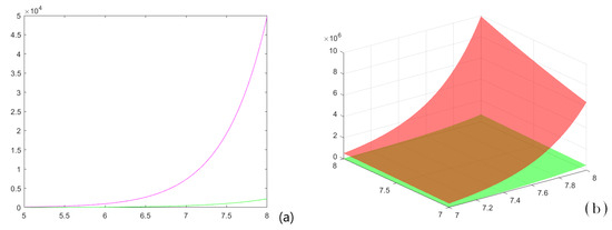
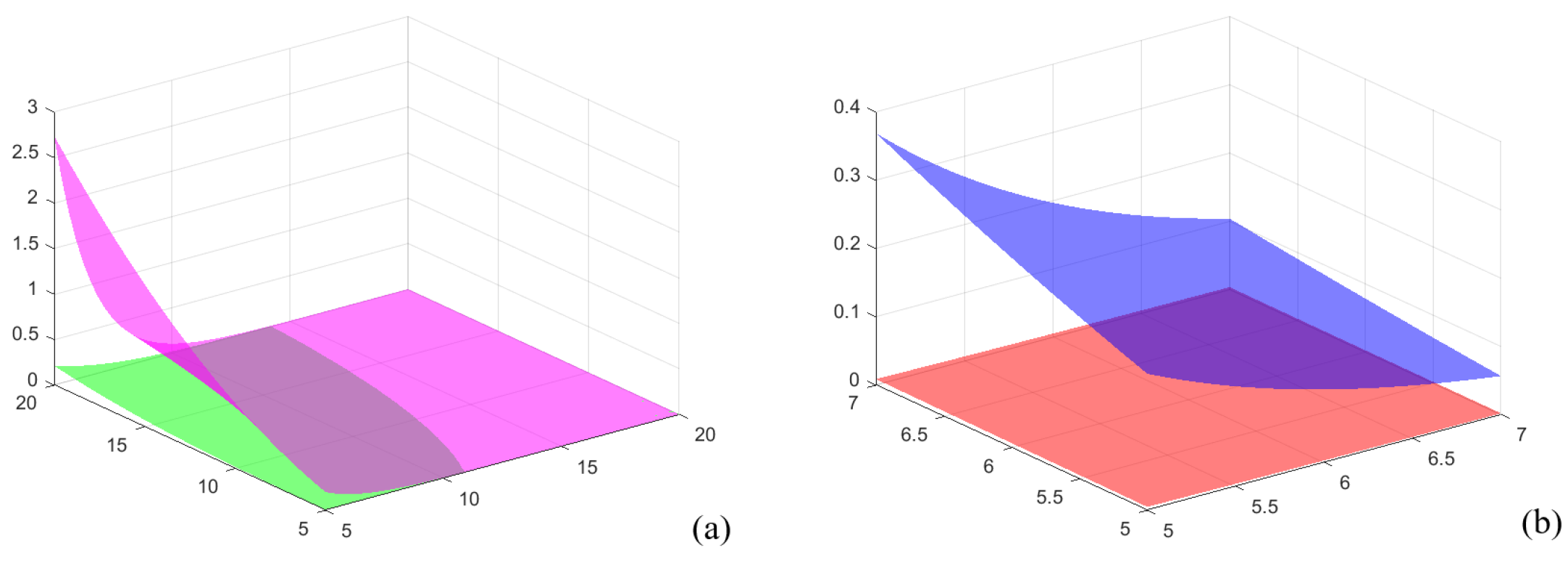
In Figure 1a, graphs of the left member (green) and the right member (magenta) of the inequality for the previously specified parameters and the function h are given.

A second numerical example with a 3-dimensional graphical representation of the left- and right-hand sides of the inequality from Theorem 6 is stated below.

Example 2. 

We assume now that in Theorem 6 we take $h:[b,c]\subset \mathbb{R}\to \mathbb{R},h\left(\theta \right)={(\theta +a_1)}^v$, $b=1,c=4$, $\omega =2,\mu =3$, and $v,a_1\in [5,8]$. It can be seen that $|h^{‴}\left(\theta \right)|=v(v-1)(v-2){(\theta +a_1)}^{v-3}$ is a convex function on $[b,c]$ and the hypothesis of Theorem 6 is satisfied.

By computing the left member and the right member of the inequality, we have

$$\begin{array}{ccc}\hfill Ms& =& |6{\int }_2^{3}h\left(\theta \right)d\theta -4h\left(\frac{5}{2}\right)-[h\left(3\right)+h\left(2\right)]|\hfill \\ & =& |6{\int }_2^3{(\theta +a_1)}^{v}d\theta -4{\left(\frac{5}{2}+a_1\right)}^v-({(3+a_1)}^v+{(2+a_1)}^v)|\hfill \\ & =& |16\frac{{(3+a_1)}^{v+1}-{(2+a_1)}^{v+1}}{v+1}-4{\left(\frac{5}{2}+a_1\right)}^v-({(3+a_1)}^v+{(2+a_1)}^v)|,\hfill \end{array}$$

and, respectively,

$$\begin{array}{ccc}\hfill Md& =& \frac{1}{96}[|h^{‴}\left(1\right)|+|h^{‴}\left(4\right)|-\frac{1}{2}\left(\right|h^{‴}\left(2\right)|+|h^{‴}\left(3\right)\left|\right)]\hfill \\ & =& \frac{v(v-1)(v-2)}{96}[{(1+a_1)}^{v-3}+{(4+a_1)}^{v-3}-\frac{1}{2}({(2+a_1)}^{v-3}+{(3+a_1)}^{v-3})].\hfill \end{array}$$

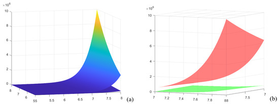
A graph of the left- and right-hand sides of the inequality from Theorem 6 when $h\left(\theta \right)=(\theta {+a_1)}^v$ and $b=1,c=4$, $\omega =2,\mu =3$, and $a_1,v\in [5,8]$ is given in Figure 2a for example 2, when the domain of definition of the represented functions is $[5,8]\times [5,8]$, which contains as a subdomain $[7,8]\times [7,8]$.

In Figure 2a,b, graph surfaces of the left member and the right member of the inequality for the previously specified parameters and function h in example 2 are given, considering functions of two variables $v,a_1\in [5,8]$ for the left member and right member.

4. Fractional Integral Hermite–Hadamard–Mercer-Type Inequalities

In this section, some Hermite–Hadamard–Mercer-type inequalities for fractional integrals for functions whose third derivative in the absolute value is convex are given.

Definition 2 

([13]). Let $h\in L_1[b,c]$. The Riemann–Liouville fractional integrals $J_{a^{+}}^{\alpha }h$ and $J_{b^{-}}^{\alpha }h$ of order $\alpha >0$, with $a\ge 0$, are defined as follows:

$$J_{a^{+}}^{\alpha }h\left(x\right)=\frac{1}{\mathsf{\Gamma }\left(\alpha \right)}{\int }_a^x{(x-t)}^{\alpha -1}h\left(t\right)dt,x>a,$$

and

$$J_{b^{-}}^{\alpha }h\left(x\right)=\frac{1}{\mathsf{\Gamma }\left(\alpha \right)}{\int }_x^b{(t-x)}^{\alpha -1}h\left(t\right)dt,x<b,$$

respectively, where Γ is the well-known gamma function.

For more important properties about fractional calculus, see the books [34,35]. In this section, we establish an integral identity in the case of differentiable functions via Riemann–Liouville fractional integrals necessary for the main results.

Lemma 2. 

Let $h:[b,c]\to \mathbb{R}$ be a three-times differentiable mapping. If h is integrable and continuous, then the following equality holds for all $\omega ,\mu \in [b,c]$, with $\omega <\mu$:

$$\begin{array}{ccc}& & \frac{\alpha (\alpha +3)}{2^{\alpha -3}{(\mu -\omega )}^3}h(b+c-\frac{\omega +\mu }{2})+\frac{1}{2^{\alpha -3}{(\mu -\omega )}^3}[h(b+c-\omega )+h(b+c-\mu )]\hfill \\ & & -\frac{4\mathsf{\Gamma }(\alpha +3)}{{(\mu -\omega )}^{\alpha +3}}[J_{{(b+c-\frac{\omega +\mu }{2})}^{+}}^{\alpha }h(b+c-\omega )+J_{{(b+c-\frac{\omega +\mu }{2})}^{-}}^{\alpha }h(b+c-\mu )]\hfill \\ & & =\frac{1}{2^{\alpha +1}}[{\int }_0^1{\theta }^2({\theta }^{\alpha }-1)h^{‴}(b+c-(\frac{\theta }{2}\omega +(1-\frac{\theta }{2})\mu ))d\theta \hfill \\ & & +{\int }_0^1{\theta }^2(1-{\theta }^{\alpha })h^{‴}(b+c-(\frac{\theta }{2}\mu +(1-\frac{\theta }{2})\omega ))d\theta ].\hfill \end{array}$$

Proof. 

By using the rule of integration and integration by parts, we obtain

$$\begin{array}{ccc}\hfill I_1& =& \frac{1}{2^{\alpha +1}}[{\int }_0^1{\theta }^2({\theta }^{\alpha }-1)h^{‴}(b+c-(\frac{\theta }{2}\omega +(1-\frac{\theta }{2})\mu ))d\theta \hfill \\ & =& \frac{1}{2^{\alpha +1}}{[\frac{2({\theta }^{\alpha +2}-{\theta }^2)}{\mu -\omega }{h}^{″}(b+c-(\frac{\theta }{2}\omega +(1-\frac{\theta }{2})\mu ))|}_0^1\hfill \\ & -& \frac{2}{\mu -\omega }{\int }_0^1((\alpha +2){\theta }^{\alpha +1}-2\theta )h^{″}(b+c-(\frac{\theta }{2}\omega +(1-\frac{\theta }{2})\mu ))d\theta ]\hfill \\ & =& -\frac{1}{2^{\alpha }(\mu -\omega )}{[\frac{2((\alpha +2){\theta }^{\alpha +1}-2\theta )}{\mu -\omega }{h}^{\prime }(b+c-(\frac{\theta }{2}\omega +(1-\frac{\theta }{2})\mu ))|}_0^1\hfill \\ & -& \frac{2}{\mu -\omega }{\int }_0^1((\alpha +2)(\alpha +1){\theta }^{\alpha }-2)h^{\prime }(b+c-(\frac{\theta }{2}\omega +(1-\frac{\theta }{2})\mu ))d\theta ]\hfill \\ & =& -\frac{\alpha }{2^{\alpha -1}{(\mu -\omega )}^2}{h}^{\prime }(b+c-\frac{\omega +\mu }{2})\hfill \\ & +& \frac{1}{2^{\alpha -2}{(\mu -\omega )}^3}{[\frac{((\alpha +2)(\alpha +1){\theta }^{\alpha }-2)}{\mu -\omega }h(b+c-(\frac{\theta }{2}\omega +(1-\frac{\theta }{2})\mu ))|}_0^1\hfill \\ & -& {\int }_0^1(\alpha +2)(\alpha +1)\alpha {\theta }^{\alpha -1}h(b+c-(\frac{\theta }{2}\omega +(1-\frac{\theta }{2})\mu ))d\theta ]\hfill \\ & =& -\frac{\alpha }{2^{\alpha -1}{(\mu -\omega )}^2}{h}^{\prime }(b+c-\frac{\omega +\mu }{2})+\frac{\alpha (\alpha +3)}{2^{\alpha -2}{(\mu -\omega )}^3}h(b+c-\frac{\omega +\mu }{2})\hfill \\ & +& \frac{1}{2^{\alpha -3}{(\mu -\omega )}^3}h(b+c-\mu )-\frac{4(\alpha +2)(\alpha +1)\alpha }{{(\mu -\omega )}^{\alpha +3}}\mathsf{\Gamma }\left(\alpha \right)J_{{(b+c-\frac{\mu +\omega }{2})}^{-}}^{\alpha }h(b+c-\mu ).\hfill \end{array}$$

Similarly, we obtain

$$\begin{array}{ccc}\hfill I_2& =& \frac{1}{2^{\alpha +1}}[{\int }_0^1{\theta }^2(1-{\theta }^{\alpha })h^{‴}(b+c-(\frac{\theta }{2}\mu +(1-\frac{\theta }{2})\omega ))d\theta \hfill \\ & =& \frac{\alpha }{2^{\alpha -1}{(\mu -\omega )}^2}{h}^{\prime }(b+c-\frac{\omega +\mu }{2})+\frac{\alpha (\alpha +3)}{2^{\alpha -2}{(\mu -\omega )}^3}h(b+c-\frac{\omega +\mu }{2})\hfill \\ & +& \frac{1}{2^{\alpha -3}{(\mu -\omega )}^3}h(b+c-\mu )-\frac{4(\alpha +2)(\alpha +1)\alpha }{{(\mu -\omega )}^{\alpha +3}}\mathsf{\Gamma }\left(\alpha \right)J_{{(b+c-\frac{\mu +\omega }{2})}^{+}}^{\alpha }h(b+c-\omega ).\hfill \end{array}$$

By adding $I_1$ to $I_2$ we have the desired identity. □

Theorem 9. 

If the hypothesis of Lemma 2 takes place and $|h^{‴}|$ satisfies inequality (3) from Theorem 1, then the following inequality holds:

$$|\frac{\alpha (\alpha +3)}{2^{\alpha -3}{(\mu -\omega )}^3}h(b+c-\frac{\omega +\mu }{2})+\frac{1}{2^{\alpha -3}{(\mu -\omega )}^3}[h(b+c-\omega )+h(b+c-\mu )]$$

$$-\frac{4\mathsf{\Gamma }(\alpha +3)}{{(\mu -\omega )}^{\alpha +3}}[J_{{(b+c-\frac{\omega +\mu }{2})}^{+}}^{\alpha }h(b+c-\omega )+J_{{(b+c-\frac{\omega +\mu }{2})}^{-}}^{\alpha }h(b+c-\mu )]|$$

(6)

$$\le \frac{\alpha }{3(\alpha +3)2^{\alpha +1}}[2(|h^{‴}\left(b\right)|+|h^{‴}\left(c\right)\left|\right)-\left(\right|h^{‴}\left(\omega \right)|+|h^{‴}\left(\mu \right)\left|\right)].$$

Proof. 

The modulus property in the identity from Lemma 2 is used, and we have

$$\begin{array}{ccc}& & |\frac{\alpha (\alpha +3)}{2^{\alpha -3}{(\mu -\omega )}^3}h(b+c-\frac{\omega +\mu }{2})+\frac{1}{2^{\alpha -3}{(\mu -\omega )}^3}[h(b+c-\omega )+h(b+c-\mu )]\hfill \\ & & -\frac{4\mathsf{\Gamma }(\alpha +3)}{{(\mu -\omega )}^{\alpha +3}}[J_{{(b+c-\frac{\omega +\mu }{2})}^{+}}^{\alpha }h(b+c-\omega )+J_{{(b+c-\frac{\omega +\mu }{2})}^{-}}^{\alpha }h(b+c-\mu )]|\hfill \\ & & \le \frac{1}{2^{\alpha +1}}[{\int }_0^1{\theta }^2(1-{\theta }^{\alpha })\left|h^{‴}(b+c-(\frac{\theta }{2}\omega +(1-\frac{\theta }{2})\mu ))\right|d\theta \hfill \\ & & +\frac{1}{2^{\alpha +1}}[{\int }_0^1{\theta }^2(1-{\theta }^{\alpha })|h^{‴}(b+c-(\frac{\theta }{2}\mu +(1-\frac{\theta }{2})\omega ))|d\theta ]\hfill \\ & & \le \frac{1}{2^{\alpha +1}}\{{\int }_0^1{\theta }^2(1-{\theta }^{\alpha })[|h^{‴}\left(b\right)|+|h^{‴}\left(c\right)|-\frac{\theta }{2}|h^{‴}\left(\omega \right)|-(1-\frac{\theta }{2})|h^{‴}\left(\mu \right)|]d\theta \hfill \\ & & +{\int }_0^1{\theta }^2(1-{\theta }^{\alpha })[|h^{‴}\left(b\right)|+|h^{‴}\left(c\right)|-\frac{\theta }{2}|h^{‴}\left(\mu \right)|-(1-\frac{\theta }{2})|h^{‴}\left(\omega \right)|]d\theta \}\hfill \\ & & \le \frac{1}{2^{\alpha +1}}\left({\int }_0^1{\theta }^2(1-{\theta }^{\alpha })d\theta \right)\{2[|h^{‴}\left(b\right)|+|h^{‴}\left(c\right)|]-|h^{‴}\left(\omega \right)|-|h^{‴}\left(\mu \right)\left|\right\}\hfill \end{array}$$

and because ${\int }_0^1{\theta }^2(1-{\theta }^{\alpha })d\theta =\frac{\alpha }{3(\alpha +3)}$, we obtain the desired inequality. □

Theorem 10. 

If the hypothesis of Lemma 2 takes place and $|h^{‴}{|}^q$, $q\ge 1$ satisfies inequality (3) from Theorem 1, then the following inequality holds:

$$\begin{array}{ccc}& & |\frac{\alpha (\alpha +3)}{2^{\alpha -3}{(\mu -\omega )}^3}h(b+c-\frac{\omega +\mu }{2})+\frac{1}{2^{\alpha -3}{(\mu -\omega )}^3}[h(b+c-\omega )+h(b+c-\mu )]\hfill \\ & & -\frac{4\mathsf{\Gamma }(\alpha +3)}{{(\mu -\omega )}^{\alpha +3}}[J_{{(b+c-\frac{\omega +\mu }{2})}^{+}}^{\alpha }h(b+c-\omega )+J_{{(b+c-\frac{\omega +\mu }{2})}^{-}}^{\alpha }h(b+c-\mu )]|\hfill \\ & & \le \frac{1}{{\alpha }^{\frac{1}{p}}{2}^{\alpha +1}}{B}^{\frac{1}{p}}(\frac{2p+1}{\alpha },p+1)[(|h^{‴}\left(b\right){|}^q+|h^{‴}\left(c\right){{|}^q-\frac{|h^{‴}{\left(\omega \right)|}^q+3{\left|h^{‴}\left(\mu \right)\right|}^q}{4})}^{\frac{1}{q}}+\hfill \\ & & +\left(\right|h^{‴}{\left(b\right)|}^q+|h^{‴}{\left(c\right)|}^q-\frac{|h^{‴}{\left(\mu \right)|}^q+3{\left|h^{‴}\left(\omega \right)\right|}^q}{4}{)}^{\frac{1}{q}}],\hfill \end{array}$$

where B is the beta function of Euler.

Proof. 

The modulus property in the identity from Lemma 2 is used, and we use the Hölder inequality and inequality (3) from Theorem 1:

$$\begin{array}{ccc}& & |\frac{\alpha (\alpha +3)}{2^{\alpha -3}{(\mu -\omega )}^3}h(b+c-\frac{\omega +\mu }{2})+\frac{1}{2^{\alpha -3}{(\mu -\omega )}^3}[h(b+c-\omega )+h(b+c-\mu )]\hfill \\ & & -\frac{4\mathsf{\Gamma }(\alpha +3)}{{(\mu -\omega )}^{\alpha +3}}[J_{{(b+c-\frac{\omega +\mu }{2})}^{+}}^{\alpha }h(b+c-\omega )+J_{{(b+c-\frac{\omega +\mu }{2})}^{-}}^{\alpha }h(b+c-\mu )]|\hfill \\ & & \le \frac{1}{2^{\alpha +1}}[{\int }_0^1{\theta }^2(1-{\theta }^{\alpha })\left|h^{‴}(b+c-(\frac{\theta }{2}\omega +(1-\frac{\theta }{2})\mu ))\right|d\theta \hfill \\ & & +\frac{1}{2^{\alpha +1}}[{\int }_0^1{\theta }^2(1-{\theta }^{\alpha })|h^{‴}(b+c-(\frac{\theta }{2}\mu +(1-\frac{\theta }{2})\omega ))|d\theta ]\hfill \\ & & \le \frac{1}{2^{\alpha +1}}{\left({\int }_0^1{\theta }^{2p}{(1-{\theta }^{\alpha })}^{p}d\theta \right)}^{\frac{1}{p}}[({\int }_0^1|h^{‴}{(b+c-(\frac{\theta }{2}\omega +(1-\frac{\theta }{2})\mu ){|}^{q}d\theta )}^{\frac{1}{q}}\hfill \end{array}$$

$$\begin{array}{ccc}& & +\left({\int }_0^1\right|h^{‴}{(b+c-(\frac{\theta }{2}\mu +(1-\frac{\theta }{2})\omega ){|}^{q}d\theta )}^{\frac{1}{q}}]\hfill \\ & & \le \frac{1}{2^{\alpha +1}{\alpha }^{\frac{1}{p}}}{\left({\int }_0^1{t}^{\frac{2p+1}{\alpha }-1}{(1-t)}^{p}dt\right)}^{\frac{1}{p}}[(|h^{‴}{\left(b\right)|}^q+|h^{‴}{\left(c\right)|}^q-{\left|h^{‴}\left(\omega \right)\right|}^q{\int }_0^1\frac{\theta }{2}d\theta \hfill \\ & & -|h^{‴}{\left(\mu \right)|}^q{\int }_0^1(1-\frac{\theta }{2}){d\theta )}^{\frac{1}{q}}+\left(\right|h^{‴}\left(b\right){|}^q+|h^{‴}\left(c\right){|}^q-{\left|h^{‴}\left(\mu \right)\right|}^q{\int }_0^1\frac{\theta }{2}d\theta \hfill \\ & & -|h^{‴}{\left(\omega \right)|}^q{\int }_0^1(1-\frac{\theta }{2})d\theta {)}^{\frac{1}{q}}].\hfill \end{array}$$

From here, by calculus we obtain the desired result. □

Theorem 11. 

If the hypothesis of Lemma 2 holds, and $|h^{‴}{|}^q$ satisfies inequality (3) from Theorem 1, where $q>1,$$\frac{1}{p}+\frac{1}{q}=1$, then we have

$$|\frac{\alpha (\alpha +3)}{2^{\alpha -3}{(\mu -\omega )}^3}h(b+c-\frac{\omega +\mu }{2})+\frac{1}{2^{\alpha -3}{(\mu -\omega )}^3}[h(b+c-\omega )+h(b+c-\mu )]$$

$$-\frac{4\mathsf{\Gamma }(\alpha +3)}{{(\mu -\omega )}^{\alpha +3}}[J_{{(b+c-\frac{\omega +\mu }{2})}^{+}}^{\alpha }h(b+c-\omega )+J_{{(b+c-\frac{\omega +\mu }{2})}^{-}}^{\alpha }h(b+c-\mu )]|$$

$$\begin{array}{ccc}& & \le \frac{1}{2^{\alpha +1}}{\left(\frac{\alpha }{3(\alpha +3)}\right)}^{1-\frac{1}{q}}[\frac{\alpha }{3(\alpha +3)}\left(\right(|h^{‴}{\left(b\right)|}^q+|h^{‴}{\left(c\right)|}^q)-\frac{\alpha }{8(\alpha +4)}{\left|h^{‴}\left(\omega \right)\right|}^q\hfill \\ & & -(\frac{5}{24}-\frac{\alpha +5}{2(\alpha +3)(\alpha +4)})|h^{‴}\left(\mu \right){|}^q{)}^{\frac{1}{q}}+(\frac{\alpha }{3(\alpha +3)}\left(\right|h^{‴}\left(b\right){|}^q+{\left|h^{‴}\left(c\right)\right|}^q)\hfill \\ & & -\frac{\alpha }{8(\alpha +4)}|h^{‴}{\left(\mu \right)|}^q-(\frac{5}{24}-\frac{\alpha +5}{2(\alpha +3)(\alpha +4)})|h^{‴}\left(\omega \right){|}^q{)}^{\frac{1}{q}}],\hfill \end{array}$$

where B is the beta function of Euler.

Proof. 

Using the modulus property, the power mean inequality, and the identity from Lemma 2, then we have

$$\begin{array}{ccc}& & |\frac{\alpha (\alpha +3)}{2^{\alpha -3}{(\mu -\omega )}^3}h(b+c-\frac{\omega +\mu }{2})+\frac{1}{2^{\alpha -3}{(\mu -\omega )}^3}[h(b+c-\omega )+h(b+c-\mu )]\hfill \\ & & -\frac{4\mathsf{\Gamma }(\alpha +3)}{{(\mu -\omega )}^{\alpha +3}}[J_{{(b+c-\frac{\omega +\mu }{2})}^{+}}^{\alpha }h(b+c-\omega )+J_{{(b+c-\frac{\omega +\mu }{2})}^{-}}^{\alpha }h(b+c-\mu )]|\hfill \\ & & \le \frac{1}{2^{\alpha +1}}[{\int }_0^1{\theta }^2(1-{\theta }^{\alpha })\left|h^{‴}(b+c-(\frac{\theta }{2}\omega +(1-\frac{\theta }{2})\mu ))\right|d\theta \hfill \\ & & +\frac{1}{2^{\alpha +1}}[{\int }_0^1{\theta }^2(1-{\theta }^{\alpha })|h^{‴}(b+c-(\frac{\theta }{2}\mu +(1-\frac{\theta }{2})\omega ))|d\theta ]\hfill \\ & & \le \frac{1}{2^{\alpha +1}}\{{\left({\int }_0^1{\theta }^2(1-{\theta }^{\alpha })d\theta \right)}^{1-\frac{1}{q}}[{\int }_0^1{\theta }^2(1-{\theta }^{\alpha })|h^{‴}(b+c-(\frac{\theta }{2}\omega +(1-\frac{\theta }{2})\mu )){{|}^{q}d\theta ]}^{\frac{1}{q}}\hfill \end{array}$$

$$\begin{array}{ccc}& & +{\left({\int }_0^1{\theta }^2(1-{\theta }^{\alpha })d\theta \right)}^{1-\frac{1}{q}}[{\int }_0^1{\theta }^2(1-{\theta }^{\alpha })|h^{‴}(b+c-(\frac{\theta }{2}\mu +(1-\frac{\theta }{2})\omega )){|}^{q}d\theta {]}^{\frac{1}{q}}\}\hfill \\ & & \le \frac{1}{2^{\alpha +1}}{\left(\frac{\alpha }{3(\alpha +3)}\right)}^{1-\frac{1}{q}}\{[\frac{\alpha }{3(\alpha +3)}\left(\right|h^{‴}{\left(b\right)|}^q+|h^{‴}\left(c\right){|}^q)\hfill \\ & & -|h^{‴}{\left(\omega \right)|}^q{\int }_0^1\frac{{\theta }^3}{2}(1-{\theta }^{\alpha })d\theta -|h^{‴}\left(\mu \right){{|}^q{\int }_0^1{\theta }^2(1-{\theta }^{\alpha })(1-\frac{\theta }{2})d\theta ]}^{\frac{1}{q}}\hfill \\ & & +[\frac{\alpha }{3(\alpha +3)}\left(\right|h^{‴}{\left(b\right)|}^q+|h^{‴}{\left(c\right)|}^q)-|h^{‴}{\left(\mu \right)|}^q{\int }_0^1\frac{{\theta }^3}{2}(1-{\theta }^{\alpha })d\theta \hfill \\ & & -|h^{‴}{\left(\omega \right)|}^q{\int }_0^1{\theta }^2(1-{\theta }^{\alpha })(1-\frac{\theta }{2})d\theta {]}^{\frac{1}{q}}\}.\hfill \end{array}$$

By easy calculus we find the right member of the desired inequality. □

Remark 7. 

If we take $\omega =b$ and $\mu =c$, then the equality from Lemma 2 can be written as follows:

$$\frac{\alpha (\alpha +3)}{2^{\alpha -3}{(c-b)}^3}h\left(\frac{b+c}{2}\right)+\frac{h\left(b\right)+h\left(c\right)}{2^{\alpha -3}{(c-b)}^3}-4\frac{\mathsf{\Gamma }(\alpha +3)}{{(c-b)}^{\alpha +3}}[J_{{\left(\frac{b+c}{2}\right)}^{+}}^{\alpha }h\left(c\right)+J_{{\left(\frac{b+c}{2}\right)}^{-}}^{\alpha }h\left(b\right)]$$

$$=\frac{1}{2^{\alpha +1}}[{\int }_0^1{\theta }^2({\theta }^{\alpha }-1)h^{‴}\left((1-\frac{\theta }{2})b+\frac{\theta }{2}c\right)d\theta +{\int }_0^1{\theta }^2(1-{\theta }^{\alpha })h^{‴}\left((1-\frac{\theta }{2})c+\frac{\theta }{2}b\right)d\theta ].$$

Remark 8. 

If we take $\alpha =1$ in Remark 7, then we obtain the equality from Remark 1.

Remark 9. 

If we take $\omega =b$ and $\mu =c$ in Theorem 9, then the inequality from there can be written as follows:

$$\begin{array}{ccc}& & |\frac{\alpha (\alpha +3)}{2^{\alpha -3}{(c-b)}^3}h\left(\frac{b+c}{2}\right)+\frac{h\left(b\right)+h\left(c\right)}{2^{\alpha -3}{(c-b)}^3}-4\frac{\mathsf{\Gamma }(\alpha +3)}{{(c-b)}^{\alpha +3}}[J_{{\left(\frac{b+c}{2}\right)}^{+}}^{\alpha }h\left(c\right)+J_{{\left(\frac{b+c}{2}\right)}^{-}}^{\alpha }h\left(b\right)]|\hfill \\ & & \le \frac{\alpha }{3(\alpha +3)2^{\alpha +1}}[|h^{‴}\left(b\right)|+|h^{‴}\left(c\right)|].\hfill \end{array}$$

Remark 10. 

If we take $\alpha =1$ in Remark 9, then we obtain the inequality from Remark 2.

Remark 11. 

If we take $\omega =b$ and $\mu =c$ in Theorem 10, then we obtain the following inequality:

$$|\frac{\alpha (\alpha +3)}{2^{\alpha -3}{(c-b)}^3}h\left(\frac{b+c}{2}\right)+\frac{h\left(b\right)+h\left(c\right)}{2^{\alpha -3}{(c-b)}^3}-4\frac{\mathsf{\Gamma }(\alpha +3)}{{(c-b)}^{\alpha +3}}[J_{{\left(\frac{b+c}{2}\right)}^{+}}^{\alpha }h\left(c\right)+J_{{\left(\frac{b+c}{2}\right)}^{-}}^{\alpha }h\left(b\right)]|$$

$$\le \frac{\alpha }{2^{\alpha +1}{\alpha }^{\frac{1}{p}}}{B}^{\frac{1}{p}}(\frac{2p+1}{\alpha },p+1)[{\left(\frac{3|h^{‴}{\left(b\right)|}^q+{\left|h^{‴}\left(c\right)\right|}^q}{4}\right)}^{\frac{1}{q}}+{\left(\frac{|h^{‴}{\left(b\right)|}^q+3{\left|h^{‴}\left(c\right)\right|}^q}{4}\right)}^{\frac{1}{q}}].$$

Remark 12. 

If we take $\alpha =1$ in Remark 11, then we obtain the inequality from Remark 4.

Remark 13. 

If we take $\omega =b$ and $\mu =c$ in Theorem 11, then we find the following inequality:

$$\begin{array}{ccc}& & |\frac{\alpha (\alpha +3)}{2^{\alpha -3}{(c-b)}^3}h\left(\frac{b+c}{2}\right)+\frac{h\left(b\right)+h\left(c\right)}{2^{\alpha -3}{(c-b)}^3}-4\frac{\mathsf{\Gamma }(\alpha +3)}{{(c-b)}^{\alpha +3}}[J_{{\left(\frac{b+c}{2}\right)}^{+}}^{\alpha }h\left(c\right)+J_{{\left(\frac{b+c}{2}\right)}^{-}}^{\alpha }h\left(b\right)]|\hfill \\ & & \le \frac{1}{2^{\alpha +1}}{\left(\frac{\alpha }{3(\alpha +3)}\right)}^{1-\frac{1}{q}}\{[\frac{\alpha (5\alpha +23)}{24(\alpha +3)(\alpha +4)}|h^{‴}{\left(b\right)|}^q+\frac{\alpha }{8(\alpha +4)}|h^{‴}\left(c\right){{|}^q]}^{\frac{1}{q}}\hfill \\ & & +[\frac{\alpha }{8(\alpha +4)}|h^{‴}{\left(b\right)|}^q+\frac{\alpha (5\alpha +23)}{24(\alpha +3)(\alpha +4)}|h^{‴}{\left(c\right)|}^q{]}^{\frac{1}{q}}\}.\hfill \end{array}$$

Remark 14. 

If we take $\alpha =1$ in Remark 13, then we obtain the equality from Remark 3.

Remark 15. 

It can be seen that for the particular case of $\alpha =1$, Lemma 2 becomes Lemma 1, Theorem 9 becomes Theorem 6, Theorem 10 becomes Theorem 8, and Theorem 11 becomes Theorem 7.

As applications to special means, the following can be mentioned:

Remark 16. 

We take $\omega =b$ and $\mu =c$, and then, we can rewrite Theorem 9 as follows:

$$\begin{array}{ccc}& & |\frac{\alpha (\alpha +3)}{2^{\alpha -3}{(c-b)}^3}h\left(\mathcal{A}(b,c)\right)+\frac{\mathcal{A}\left(h\right(b),h(c\left)\right)}{2^{\alpha -4}{(c-b)}^3}-8\frac{\mathsf{\Gamma }(\alpha +3)}{{(c-b)}^{\alpha +3}}\mathcal{A}(J_{{\left(\mathcal{A}(b,c)\right)}^{+}}^{\alpha }h\left(c\right),J_{{\left(\mathcal{A}(b,c)\right)}^{-}}^{\alpha }h\left(b\right)|\hfill \\ & & \le \frac{\alpha }{3(\alpha +3)2^{\alpha }}\mathcal{A}(h^{‴}\left(b\right),h^{‴}\left(c\right)),\hfill \end{array}$$

where $\mathcal{A}(b,c)$ is the arithmetic mean of b and c.

Example 3. 

Now, we put into Theorem 9, $h:[b,c]\subset \mathbb{R}\to \mathbb{R},h\left(\theta \right)=\frac{{(\theta +a_1)}^5}{60}$, $b=0,c=1$, $\omega =\frac{1}{3},\mu =\frac{2}{3}$, and $\alpha \in [5,20]$; we see that $|h^{‴}\left(\theta \right)|={(\theta +a_1)}^2$ is a convex function and the conditions of Theorem 9 are satisfied.

Computing the left member and the right member of inequality (6), we find, successively,

$$Ms=|\frac{27\alpha (\alpha +3)}{2^{\alpha -3}}h\left(\frac{1}{2}\right)+\frac{27}{2^{\alpha -3}}[h\left(\frac{2}{3}\right)+h\left(\frac{1}{3}\right)]-4\mathsf{\Gamma }(\alpha +3)3^{\alpha +3}[J_{{\frac{1}{2}}^{+}}^{\alpha }h\left(\frac{2}{3}\right)+J_{{\frac{1}{2}}^{-}}^{\alpha }h\left(\frac{1}{3}\right)]|$$

$$\begin{array}{ccc}& & =|\frac{9}{20·2^{\alpha -3}}[{(a_1+\frac{2}{3})}^5+{(a_1+\frac{1}{3})}^5+\alpha (\alpha +3){(a_1+\frac{1}{2})}^5]\hfill \\ & & -4·3^{\alpha +3}\frac{\mathsf{\Gamma }(\alpha +3)}{\mathsf{\Gamma }\left(\alpha \right)}[{\int }_{\frac{1}{2}}^{\frac{2}{3}}{(\frac{2}{3}-t)}^{\alpha -1}\frac{{(t+a_1)}^5}{60}dt+{\int }_{\frac{1}{3}}^{\frac{1}{2}}{(t-\frac{1}{3})}^{\alpha -1}\frac{{(t+a_1)}^5}{60}dt]|,\hfill \end{array}$$

and, respectively,

$$Md=\frac{\alpha }{3(\alpha +3)2^{\alpha +1}}[2a_1^2+2{(1+a_1)}^2-{(a_1+\frac{1}{3})}^2-{(a_1+\frac{2}{3})}^2].$$

Some calculus from these examples and all the figures were made using the Matlab R2023b software.

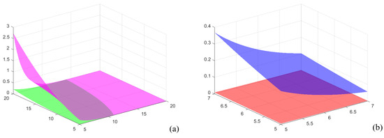
In Figure 3a, graph surfaces of the left member (green) and the right member (magenta) of inequality (6) are given for the previously specified parameters and function h, and in Figure 3b graphs of the left member (red) and the right member (blue) of inequality (6) for the previously specified parameters and function h are given, but for when $\alpha ,a_1\in [5,8]$. We considered here functions of two variables α and $a_1$ for the surfaces.

A second numerical example, as a particular case of the previous example, when $a_1=0$ and $\alpha \in [5,10]$ with a 2-dimensional graphical representation, is presented below.

Example 4. 

We assume now that in Theorem 9 we take $h:[b,c]\subset \mathbb{R}\to \mathbb{R},h\left(\theta \right)=\frac{{\theta }^5}{60}$, $b=0,c=1$, $\omega =\frac{1}{3},\mu =\frac{2}{3}$, and $\alpha \in [5,10]$. It can be seen that $|h^{‴}\left(\theta \right)|={\theta }^2$ is a convex function and the hypothesis of Theorem 9 is satisfied.

Computing the left member and the right member of inequality (6), we obtain

$$\begin{array}{ccc}\hfill Ms& =& |\frac{9}{20·2^{\alpha -3}}[{\left(\frac{2}{3}\right)}^5+{\left(\frac{1}{3}\right)}^5+\alpha (\alpha +3){\left(\frac{1}{2}\right)}^5]\hfill \\ & -& \frac{3^{\alpha +2}(\alpha +2)(\alpha +1)\alpha }{5}[{\int }_{\frac{1}{2}}^{\frac{2}{3}}{(\frac{2}{3}-t)}^{\alpha -1}{t}^{5}dt+{\int }_{\frac{1}{3}}^{\frac{1}{2}}{(t-\frac{1}{3})}^{\alpha -1}{t}^{5}dt]|,\hfill \end{array}$$

and, respectively,

$$Md=\frac{13\alpha }{27(\alpha +3)2^{\alpha +1}}.$$

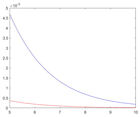
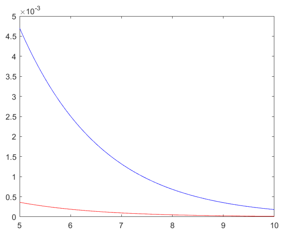
In Figure 4, graphs of the left member (red line) and of the right member (blue line) of the inequality (6) are given for the previously specified parameters and function h, considering functions of one variable, α, for the left member and right member.

The k-Riemann–Liouville fractional integrals ${}_{k}J_{a^{+}}^{\alpha }h$ can be seen as a generalization of Riemann–Liouville fractional integrals with a parameter k.

Definition 3 

([16,36]). “Let $h\in L_1[b,c]$. The k-Riemann–Liouville fractional integrals ${}_{k}J_{a^{+}}^{\alpha }h$ and ${}_{k}J_{b^{-}}^{\alpha }h$ of order α, where $k>0$, with $a\ge 0$, are defined as follows:

$${}_{k}J_{a^{+}}^{\alpha }h\left(x\right)=\frac{1}{k{\mathsf{\Gamma }}_k\left(\alpha \right)}{\int }_a^x{(x-t)}^{\frac{\alpha }{k}-1}h\left(t\right)dt,x>a,$$

and

$${}_{k}J_{b^{-}}^{\alpha }h\left(x\right)=\frac{1}{k{\mathsf{\Gamma }}_k\left(\alpha \right)}{\int }_x^b{(t-x)}^{\frac{\alpha }{k}-1}h\left(t\right)dt,x<b,$$

respectively, where ${\mathsf{\Gamma }}_k\left(x\right)={\int }_0^{\infty }{t}^{x-1}{e}^{-\frac{t^k}{k}}dt,x>0$”.

An analogous integral identity in the case of differentiable functions via k-Riemann–Liouville fractional integrals is the following:

Remark 17. 

Let $h:[b,c]\to \mathbb{R}$ be a three-times differentiable mapping. If h is integrable and continuous, then the following equality holds for all $\omega ,\mu \in [b,c]$, with $\omega <\mu$:

$$\begin{array}{ccc}& & \frac{\alpha }{k}(\frac{\alpha }{k}+3)\frac{1}{2^{\frac{\alpha }{k}-3}{(\mu -\omega )}^3}h(b+c-\frac{\omega +\mu }{2})+\frac{1}{2^{\frac{\alpha }{k}-3}{(\mu -\omega )}^3}[h(b+c-\omega )+h(b+c-\mu )]\hfill \\ & & -\frac{4{\mathsf{\Gamma }}_k(\alpha +3k)}{k^2{(\mu -\omega )}^{\frac{\alpha }{k}+3}}[{}_{k}J_{{(b+c-\frac{\omega +\mu }{2})}^{+}}^{\alpha }h(b+c-\omega )+{}_{k}J_{{(b+c-\frac{\omega +\mu }{2})}^{-}}^{\alpha }h(b+c-\mu )]\hfill \\ & & =\frac{1}{2^{\frac{\alpha }{k}+1}}[{\int }_0^1{\theta }^2({\theta }^{\frac{\alpha }{k}}-1)h^{‴}(b+c-(\frac{\theta }{2}\omega +(1-\frac{\theta }{2})\mu ))d\theta \hfill \\ & & +{\int }_0^1{\theta }^2(1-{\theta }^{\frac{\alpha }{k}})h^{‴}(b+c-(\frac{\theta }{2}\mu +(1-\frac{\theta }{2})\omega ))d\theta ].\hfill \end{array}$$

Proof. 

The demonstration is similar to Lemma 2. □

The following results present some Hermite–Hadamard–Mercer inequalities for k-Riemann–Liouville fractional integrals for functions whose third derivative in the absolute value is convex.

Remark 18. 

If the hypothesis of Remark 17 takes place and $|h^{‴}|$ satisfies inequality (3) from Theorem 1, then the following inequality holds:

$$\begin{array}{ccc}& & |\frac{\alpha }{k}(\frac{\alpha }{k}+3)\frac{1}{2^{\frac{\alpha }{k}-3}{(\mu -\omega )}^3}h(b+c-\frac{\omega +\mu }{2})+\frac{1}{2^{\frac{\alpha }{k}-3}{(\mu -\omega )}^3}[h(b+c-\omega )+h(b+c-\mu )]\hfill \\ & & -\frac{4{\mathsf{\Gamma }}_k(\alpha +3k)}{k^2{(\mu -\omega )}^{\frac{\alpha }{k}+3}}[{}_{k}J_{{(b+c-\frac{\omega +\mu }{2})}^{+}}^{\alpha }h(b+c-\omega )+{}_{k}J_{{(b+c-\frac{\omega +\mu }{2})}^{-}}^{\alpha }h(b+c-\mu )]|\hfill \\ & & \le \frac{\alpha }{3(\alpha +3k)2^{\frac{\alpha }{k}+1}}[2(|h^{‴}\left(b\right)|+|h^{‴}\left(c\right)\left|\right)-\left(\right|h^{‴}\left(\omega \right)|+|h^{‴}\left(\mu \right)\left|\right)].\hfill \end{array}$$

Proof. 

The demonstration is similar to Theorem 9. □

Remark 19. 

If the hypothesis of Remark 17 takes place and $|h^{‴}{|}^q$, $q\ge 1$ satisfies inequality (3) from Theorem 1, then the following inequality holds:

$$\begin{array}{c}|\frac{\alpha }{k}(\frac{\alpha }{k}+3)\frac{1}{2^{\frac{\alpha }{k}-3}{(\mu -\omega )}^3}h(b+c-\frac{\omega +\mu }{2})+\frac{1}{2^{\frac{\alpha }{k}-3}{(\mu -\omega )}^3}[h(b+c-\omega )+h(b+c-\mu )]\hfill \\ -\frac{4{\mathsf{\Gamma }}_k(\alpha +3k)}{k^2{(\mu -\omega )}^{\frac{\alpha }{k}+3}}[{}_{k}J_{{(b+c-\frac{\omega +\mu }{2})}^{+}}^{\alpha }h(b+c-\omega )+{}_{k}J_{{(b+c-\frac{\omega +\mu }{2})}^{-}}^{\alpha }h(b+c-\mu )]|\hfill \\ \le {\left(\frac{k}{\alpha }\right)}^{\frac{1}{p}}{B}^{\frac{1}{p}}((2p+1)\frac{k}{\alpha },p+1)[(|h^{‴}\left(b\right){|}^q+|h^{‴}\left(c\right){{|}^q-\frac{|h^{‴}{\left(\omega \right)|}^q+3{\left|h^{‴}\left(\mu \right)\right|}^q}{4})}^{\frac{1}{q}}\hfill \\ +\left(\right|h^{‴}{\left(b\right)|}^q+|h^{‴}{\left(c\right)|}^q-\frac{|h^{‴}{\left(\mu \right)|}^q+3{\left|h^{‴}\left(\omega \right)\right|}^q}{4}{)}^{\frac{1}{q}}],\hfill \end{array}$$

where B is the beta function of Euler.

Proof. 

The demonstration is similar to Theorem 10. □

Remark 20. 

If the hypothesis of Remark 17 holds, and $|h^{‴}{|}^q$ satisfies inequality (3) from Theorem 1, where $q>1,$$\frac{1}{p}+\frac{1}{q}=1$, then we have

$$\begin{array}{ccc}& & |\frac{\alpha }{k}(\frac{\alpha }{k}+3)\frac{1}{2^{\frac{\alpha }{k}-3}{(\mu -\omega )}^3}h(b+c-\frac{\omega +\mu }{2})+\frac{1}{2^{\frac{\alpha }{k}-3}{(\mu -\omega )}^3}[h(b+c-\omega )+h(b+c-\mu )]\hfill \\ & & -\frac{4{\mathsf{\Gamma }}_k(\alpha +3k)}{k^2{(\mu -\omega )}^{\frac{\alpha }{k}+3}}[{}_{k}J_{{(b+c-\frac{\omega +\mu }{2})}^{+}}^{\alpha }h(b+c-\omega )+{}_{k}J_{{(b+c-\frac{\omega +\mu }{2})}^{-}}^{\alpha }h(b+c-\mu )]|\hfill \end{array}$$

$$\begin{array}{ccc}& \le & \frac{1}{2^{\frac{\alpha }{k}+1}}{\left(\frac{\alpha }{3(\alpha +3k)}\right)}^{1-\frac{1}{q}}[(\frac{\alpha }{3(\alpha +3k)}\left(\right|h^{‴}{\left(b\right)|}^q+|h^{‴}{\left(c\right)|}^q)-\frac{\alpha }{8(\alpha +4k)}{\left|h^{‴}\left(\omega \right)\right|}^q\hfill \\ & & -\frac{\alpha (5\alpha +23k)}{24(\alpha +3k)(\alpha +4k)}|h^{‴}{\left(\mu \right)|}^q{)}^{\frac{1}{q}}+(\frac{\alpha }{3(\alpha +3k)}\left(\right|h^{‴}{\left(b\right)|}^q+{\left|h^{‴}\left(c\right)\right|}^q)\hfill \\ & & -\frac{\alpha }{8(\alpha +4k)}|h^{‴}{\left(\mu \right)|}^q-\frac{\alpha (5\alpha +23k)}{24(\alpha +3k)(\alpha +4k)}|h^{‴}{\left(\omega \right)|}^q{)}^{\frac{1}{q}}],\hfill \end{array}$$

where B is the beta function of Euler.

Proof. 

The demonstration is similar to Theorem 11. □

Remark 21. 

Let $h:[b,c]\to \mathbb{R}$ be an n-times differentiable mapping, $n\in \mathbf{N},n\ge 3$. If h is integrable and continuous, then the following equality holds for all $\omega ,\mu \in [b,c]$, with $\omega <\mu$:

$$\begin{array}{ccc}& & \sum _{k=2}^{n-1}\frac{{(-1)}^{k-1}+1}{{(\mu -\omega )}^k}{2}^k[\frac{\mathsf{\Gamma }(\alpha +n)}{\mathsf{\Gamma }(\alpha +n-(k-1\left)\right)}-\frac{\mathsf{\Gamma }\left(n\right)}{\mathsf{\Gamma }(n-(k-1\left)\right)}]h^{(n-k)}(b+c-\frac{\omega +\mu }{2})\hfill \\ & & +\frac{2^n[{(-1)}^{n-1}+1]}{{(\mu -\omega )}^n}[\frac{\mathsf{\Gamma }(\alpha +n)}{\mathsf{\Gamma }(\alpha +1)}-\mathsf{\Gamma }\left(n\right)]h(b+c-\frac{\omega +\mu }{2})\hfill \\ & & +\frac{2^n\mathsf{\Gamma }\left(n\right)}{{(\mu -\omega )}^n}[{(-1)}^{n-1}h(b+c-\mu )+h(b+c-\omega )]\hfill \\ & & -\frac{2^{\alpha +n}\mathsf{\Gamma }(\alpha +n)}{{(\mu -\omega )}^{\alpha +n}}[{(-1)}^{n-1}{J}_{{(b+c-\frac{\omega +\mu }{2})}^{-}}^{\alpha }h(b+c-\mu )+J_{{(b+c-\frac{\omega +\mu }{2})}^{+}}^{\alpha }h(b+c-\omega )]\hfill \\ & & ={\int }_0^1{\theta }^{n-1}({\theta }^{\alpha }-1)h^{\left(n\right)}(b+c-(\frac{\theta }{2}\omega +(1-\frac{\theta }{2})\mu ))d\theta \hfill \\ & & +{\int }_0^1{\theta }^{n-1}(1-{\theta }^{\alpha })h^{\left(n\right)}(b+c-(\frac{\theta }{2}\mu +(1-\frac{\theta }{2})\omega ))d\theta .\hfill \end{array}$$

Proof. 

The demonstration is similar to Lemma 2. □

Remark 22. 

If we put $n=3$ into Remark 21, we obtain Lemma 2.

Remark 23. 

If the hypothesis of Remark 21 takes place and $|h^{\left(n\right)}|$ satisfies inequality (3) from Theorem 1, then the following inequality holds:

$$\begin{array}{ccc}& & |\sum _{k=2}^{n-1}\frac{{(-1)}^{k-1}+1}{{(\mu -\omega )}^k}{2}^k[\frac{\mathsf{\Gamma }(\alpha +n)}{\mathsf{\Gamma }(\alpha +n-(k-1\left)\right)}-\frac{\mathsf{\Gamma }\left(n\right)}{\mathsf{\Gamma }(n-(k-1\left)\right)}]h^{(n-k)}(b+c-\frac{\omega +\mu }{2})\hfill \\ & & +\frac{2^n[{(-1)}^{n-1}+1]}{{(\mu -\omega )}^n}[\frac{\mathsf{\Gamma }(\alpha +n)}{\mathsf{\Gamma }(\alpha +1)}-\mathsf{\Gamma }\left(n\right)]h(b+c-\frac{\omega +\mu }{2})\hfill \\ & & +\frac{2^n\mathsf{\Gamma }\left(n\right)}{{(\mu -\omega )}^n}[{(-1)}^{n-1}h(b+c-\mu )+h(b+c-\omega )]\hfill \\ & & -\frac{2^{\alpha +n}\mathsf{\Gamma }(\alpha +n)}{{(\mu -\omega )}^{\alpha +n}}[{(-1)}^{n-1}{J}_{{(b+c-\frac{\omega +\mu }{2})}^{-}}^{\alpha }h(b+c-\mu )+J_{{(b+c-\frac{\omega +\mu }{2})}^{+}}^{\alpha }h(b+c-\omega )]|\hfill \\ & & \le \frac{\alpha }{n(\alpha +n)}[2(|h^{\left(n\right)}\left(b\right)|+|h^{\left(n\right)}\left(c\right)\left|\right)-\left(\right|h^{\left(n\right)}\left(\omega \right)|+|h^{\left(n\right)}\left(\mu \right)\left|\right)].\hfill \end{array}$$

Remark 24. 

If the hypothesis of Remark 21 takes place and $|h^{\left(n\right)}{|}^q$, $q\ge 1$ satisfies inequality (3) from Theorem 1, then the following inequality holds:

$$\begin{array}{ccc}& & |\sum _{k=2}^{n-1}\frac{{(-1)}^{k-1}+1}{{(\mu -\omega )}^k}{2}^k[\frac{\mathsf{\Gamma }(\alpha +n)}{\mathsf{\Gamma }(\alpha +n-(k-1\left)\right)}-\frac{\mathsf{\Gamma }\left(n\right)}{\mathsf{\Gamma }(n-(k-1\left)\right)}]h^{(n-k)}(b+c-\frac{\omega +\mu }{2})\hfill \\ & & +\frac{2^n[{(-1)}^{n-1}+1]}{{(\mu -\omega )}^n}[\frac{\mathsf{\Gamma }(\alpha +n)}{\mathsf{\Gamma }(\alpha +1)}-\mathsf{\Gamma }\left(n\right)]h(b+c-\frac{\omega +\mu }{2})\hfill \\ & & +\frac{2^n\mathsf{\Gamma }\left(n\right)}{{(\mu -\omega )}^n}[{(-1)}^{n-1}h(b+c-\mu )+h(b+c-\omega )]\hfill \\ & & -\frac{2^{\alpha +n}\mathsf{\Gamma }(\alpha +n)}{{(\mu -\omega )}^{\alpha +n}}[{(-1)}^{n-1}{J}_{{(b+c-\frac{\omega +\mu }{2})}^{-}}^{\alpha }h(b+c-\mu )+J_{{(b+c-\frac{\omega +\mu }{2})}^{+}}^{\alpha }h(b+c-\omega )]|\hfill \\ & & \le \frac{1}{{\alpha }^{\frac{1}{p}}}{B}^{\frac{1}{p}}(\frac{n(p-1)+1}{\alpha },p+1)[(|h^{\left(n\right)}\left(b\right){|}^q+|h^{\left(n\right)}\left(c\right){{|}^q-\frac{|h^{\left(n\right)}{\left(\omega \right)|}^q+3{\left|h^{\left(n\right)}\left(\mu \right)\right|}^q}{4})}^{\frac{1}{q}}+\hfill \\ & & +\left(\right|h^{\left(n\right)}{\left(b\right)|}^q+|h^{\left(n\right)}{\left(c\right)|}^q-\frac{|h^{\left(n\right)}{\left(\mu \right)|}^q+3{\left|h^{\left(n\right)}\left(\omega \right)\right|}^q}{4}{)}^{\frac{1}{q}}],\hfill \end{array}$$

where B is the beta function of Euler.

Remark 25. 

If the hypothesis of Remark 21 holds, and $|h^{\left(n\right)}{|}^q$ satisfies inequality (3) from Theorem 1, where $q>1,$$\frac{1}{p}+\frac{1}{q}=1$, then we have

$$\begin{array}{ccc}& & |\sum _{k=2}^{n-1}\frac{{(-1)}^{k-1}+1}{{(\mu -\omega )}^k}{2}^k[\frac{\mathsf{\Gamma }(\alpha +n)}{\mathsf{\Gamma }(\alpha +n-(k-1\left)\right)}-\frac{\mathsf{\Gamma }\left(n\right)}{\mathsf{\Gamma }(n-(k-1\left)\right)}]h^{(n-k)}(b+c-\frac{\omega +\mu }{2})\hfill \\ & & +\frac{2^n[{(-1)}^{n-1}+1]}{{(\mu -\omega )}^n}[\frac{\mathsf{\Gamma }(\alpha +n)}{\mathsf{\Gamma }(\alpha +1)}-\mathsf{\Gamma }\left(n\right)]h(b+c-\frac{\omega +\mu }{2})\hfill \\ & & +\frac{2^n\mathsf{\Gamma }\left(n\right)}{{(\mu -\omega )}^n}[{(-1)}^{n-1}h(b+c-\mu )+h(b+c-\omega )]\hfill \\ & & -\frac{2^{\alpha +n}\mathsf{\Gamma }(\alpha +n)}{{(\mu -\omega )}^{\alpha +n}}[{(-1)}^{n-1}{J}_{{(b+c-\frac{\omega +\mu }{2})}^{-}}^{\alpha }h(b+c-\mu )+J_{{(b+c-\frac{\omega +\mu }{2})}^{+}}^{\alpha }h(b+c-\omega )]|\hfill \\ & & \le {\left(\frac{\alpha }{n(\alpha +n)}\right)}^{1-\frac{1}{q}}[(\frac{\alpha }{n(\alpha +n)}\left(\right|h^{\left(n\right)}{\left(b\right)|}^q+|h^{\left(n\right)}{\left(c\right)|}^q)-\frac{\alpha }{2(n+1)(\alpha +n+1)}{\left|h^{\left(n\right)}\left(\omega \right)\right|}^q\hfill \\ & & -(\frac{\alpha }{n(n+\alpha )}-\frac{\alpha }{2(n+1)(n+\alpha +1)})|h^{\left(n\right)}\left(\mu \right){|}^q{)}^{\frac{1}{q}}+(\frac{\alpha }{n(\alpha +n)}\left(\right|h^{\left(n\right)}\left(b\right){|}^q+{\left|h^{\left(n\right)}\left(c\right)\right|}^q)\hfill \\ & & -\frac{\alpha }{2(n+1)(\alpha +n+1)}|h^{\left(n\right)}{\left(\mu \right)|}^q-(\frac{\alpha }{n(n+\alpha )}-\frac{\alpha }{2(n+1)(n+\alpha +1)})|h^{\left(n\right)}\left(\omega \right){|}^q{)}^{\frac{1}{q}}],\hfill \end{array}$$

where B is the beta function of Euler.

5. Discussion and Conclusions

In this paper, new Hermite–Hadamard–Mercer-type inequalities are given for three-times differentiable convex functions. These results are generalizations of some inequalities existing in the literature. In addition, some applications to special means have been presented in order to verify their usefulness. In addition, several Hermite–Hadamard–Mercer-type inequalities for fractional integrals are presented by using the Jensen–Mercer inequality for three-times differentiable functions for which the absolute values of the third derivatives are convex. Some examples are given and the figures illustrate the validity of the obtained results. For the figures the Matlab R2023b software was used.

The novelty of the approach consists in the fact that the two posited lemmas represent new equalities that pave the way for the establishment of new H-H-M-type inequalities for the respective types of functions from the two main sections of the article. The methods are contained in the two lemmas.

The use of the Jensen–Mercer inequality makes the results more general than those previously studied and they can be obtained through the particularizations of the variables $\omega$ and $\mu$. Moreover, several customizations can be made that can lead to other H-H-M-type inequalities. In addition, new H-H-M-type inequalities have been established for the case when instead of the function h we have its $n^{th}$ derivative, by using first a key lemma, and also for k-Riemann–Liouville fractional integrals, too.

In addition, four examples are presented here in which the functions in these cases have one and two parameters, which allows us to graphically represent the two members of the inequalities (the left member and the right member) from Theorem 7, both in plane and in space.

The obtained results could also be useful in the case of the analysis of symmetric functions. The results we reached in this study pave the way for further research. For example, the results could be extended to quantum and post-quantum calculus.

The presented results contribute to the development of the theory of inequalities and can initiate possible applications in the field of differential equations for determining the uniqueness of solutions in fractional boundary value problems as well as in the field of information theory.

References

- Alomari, M.; Darus, M.; Kirmaci, U.S. Some inequalities of Hermite-Hadamard type for s-convex functions. Acta Math. Sci. 2011, 8, 1643–1652. [Google Scholar] [CrossRef]
- Ekinci, A.; Akdemir, A.O.; Ozdemir, M.E. Integral inequalities for different kinds of convexity via classical inequalities. Turk. J. Sci. 2020, 5, 305–313. [Google Scholar]
- Khan, A.; Chu, Y.M.; Khan, T.U.; Khan, J. Some inequalities of Hermite-Hadamard type for s-convex functions with applications. Open Math. 2017, 15, 1414–1430. [Google Scholar] [CrossRef]
- Ozdemir, M.E.; Ekinci, A.; Akdemir, A.O. Some new integral inequalities for functions whose derivatives of absolute values are convex and concave. TWMS J. Pure Appl. Math. 2019, 2, 212–224. [Google Scholar]
- Barsam, H.; Ramezani, S.M.; Sayyari, Y. On the new Hermite-Hadamard type inequalities for s-convex functions. Afr. Mat. 2021, 32, 1355–1367. [Google Scholar] [CrossRef]
- Barsam, H.; Sattarzadeh, A.R. Hermite-Hadamard inequalities for uniformly convex functions and its applications in means. Miskolc Math. Notes 2020, 2, 1787–2413. [Google Scholar] [CrossRef]
- Dragomir, S.S.; Pearce, C.E.M. Selected topic on Hermite-Hadamard inequalities and applications. Melb. Adel. 2001, 4, S1574-0358. [Google Scholar]
- Dragomir, S.S.; Fitzpatrick, S. The Hadamard’s inequality for s-convex functionsin the second sense. Demonstratio Math. 1999, 32, 687–696. [Google Scholar]
- Butt, S.I.; Nadeem, M.; Farid, G. On Caputo fractional derivatives via exponential s-convex functions. Turk. J. Sci. 2020, 5, 140–146. [Google Scholar]
- Latif, M.A.; Kunt, M.; Dragomir, S.S.; Iscan, I. Post-quantum trapezoid type inequalities. AIMS Math. 2020, 5, 4011–4026. [Google Scholar] [CrossRef]
- Kunt, M.; Iscan, I. Fractional Hermite-Hadamard-Fejer type inequalities for GA-convex functions. Turk. J. Inequal. 2018, 2, 1–20. [Google Scholar]
- Luangboon, W.; Nonlaopon, K.; Tariboon, J.; Ntouyas, S.K.; Budak, H. Post-Quantum Ostrowski type integral inequalities for two (p,q)-differentiable functions. J. Math. Ineq. 2022, 16, 1129–1144. [Google Scholar] [CrossRef]
- Sitthiwirattham, T.; Viva-Cortes, M.; Ali, M.A.; Budak, H. A study of fractional Hermite-Hadamard-Mercer inequalities for differentiable functions. Fractals 2024, 32, 13. [Google Scholar] [CrossRef]
- Alp, N.; Budak, H.; Sarikaya, M.Z.; Ali, M.A. On new refinements and generalizations of q-Hermite-Hadamard inequalities for convex functions. Rocky Mt. J. Math. 2023, 54, 361–374. [Google Scholar] [CrossRef]
- Sarikaya, M.Z.; Kiris, M.E. Some new inequalities of Hermite-Hadamard-type for s-convex functions. Miskolc Math. Notes 2015, 16, 491–501. [Google Scholar] [CrossRef]
- Ramezan, S.; Awan, M.U.; Dragomir, S.S.; Bin-Mohsin, B.; Noor, M.A. Analysis and Applications of some new fractional integral inequalities. Fractal Fract. 2023, 7, 797. [Google Scholar] [CrossRef]
- Sahoo, S.K.; Kashuri, A.; Aljuaid, M.; Mishra, S.; De la Sen, M. On Ostrowski-Mercer type fractional inequalities for convex functions and applications. Fractal Fract. 2023, 7, 215. [Google Scholar] [CrossRef]
- Park, J. Hermite-Hadamard-like Type Inequalities for s-Convex Functions and s-Godunova-Levin Functions of two kinds. Appl. Math. Sci. 2015, 69, 3431–3447. [Google Scholar] [CrossRef]
- Ciurdariu, L. Some Hermite-Hadamard type inequalities involving fractional integral operators. J. Sci. Arts 2022, 22, 941–952. [Google Scholar] [CrossRef]
- Ciurdariu, L.; Grecu, E. Several quantum Hermite-Hadamard-type integral inequalities for convex functions. Fractal Fract. 2023, 7, 463. [Google Scholar] [CrossRef]
- Hadamard, J. Etude sur le proprietes des fonctions entieres en particulier d’ une fonction consideree par Riemann. J. Math. Pures Appl. 1893, 58, 171–215. [Google Scholar]
- Hermite, C. Sur deux limites d’une integrale definie. Mathesis 1883, 3, 382. [Google Scholar]
- Mercer, A.M. A variant of Jensen’s inequality. J. Inequalities Pure Appl. Math. 2003, 4, 73. [Google Scholar]
- Khan, M.A.; Husain, Z.; Chu, Y.M. New estimates for Csiszar divergence and Zipf-Mandelbrot entropy via Jensen-Mercer’s inequality. Complexity 2022, 2020, 8928691. [Google Scholar]
- Kian, M.; Moslehian, M.S. Refinements of the operator Jensen-Mercer inequality. Electron. J. Linear Algebra 2013, 26, 742–753. [Google Scholar] [CrossRef]
- Wang, H.; Khan, J.; Khan, M.A.; Khalid, S.; Khan, R. The Hermite-Hadamard-Jensen-Mercer-type inequalities for Riemann Liouville fractional integral. J. Math. 2021, 2021, 5516987. [Google Scholar] [CrossRef]
- Abdeljawad, T.; Ali, M.A.; Mohammed, P.O.; Kashuri, A. On inequalities of Hermite-Hadamard-Mercer-type involving Riemann-Liouville fractional integrals. AIMS Math. 2021, 6, 712–725. [Google Scholar] [CrossRef]
- Chu, H.H.; Rashid, S.; Hammouch, Z.; Chu, Y.M. New fractional estimates for Hermite-Hadamard-Mercer’s type inequalities. Alex. Eng. J. 2020, 59, 3079–3089. [Google Scholar] [CrossRef]
- Set, E.; Celik, B.; Ozdemir, M.E.; Aslan, M. Some new results on Hermite-Hadamard-Mercer-type inequality using a general family of fractional integral operators. Fractal Fract. 2021, 5, 68. [Google Scholar] [CrossRef]
- Sial, I.B.; Patanarapeelert, N.; Ali, M.A.; Budak, H.; Sitthiwirattham, T. On some new Ostrowski-Mercer-type inequalities for differentiable functions. Axioms 2022, 11, 132. [Google Scholar] [CrossRef]
- Kara, H.; Ali, M.A.; Budak, H. Hermite-Hadamard-Mercer-type inclusions for interval valued functions via Riemann-Liouville fractional integrals. Turk. J. Math. 2022, 46, 2193–2207. [Google Scholar] [CrossRef]
- Butt, S.I.; Yousaf, S.; Asghar, A.; Khan, K.A.; Moraldi, H.R. New fractional Hermite-Hadamard-Mercer inequalities for harmonically convex function. J. Funct. Spaces 2021, 2021, 5868326. [Google Scholar] [CrossRef]
- Ali, M.A.; Sitthiwirattham, T.; Kobis, E.; Hanif, A. Hermite-Hadamard-Mercer inequalities associated with twice-differentiable functions with applications. Axioms 2024, 13, 114. [Google Scholar] [CrossRef]
- Gorenflo, R.; Mainardi, F. Fractional Calculus: Integral and Differential Equations of Fractional Order; Springer: Berlin/Heidelberg, Germany, 1997. [Google Scholar]
- Kilbas, A.A.; Srivastava, H.M.; Trujillo, J.J. Theory and Applications of Fractional Differential Equations, North-Holland Mathematics Studies; Elsevier: Amsterdam, The Netherlands, 2006; Volume 20. [Google Scholar]
- Mubeen, S.; Habibullah, G.M. k-Fractional integrals and applications. Int. J. Contemp. Math. 2012, 7, 89–94. [Google Scholar]
Disclaimer/Publisher’s Note: The statements, opinions and data contained in all publications are solely those of the individual author(s) and contributor(s) and not of MDPI and/or the editor(s). MDPI and/or the editor(s) disclaim responsibility for any injury to people or property resulting from any ideas, methods, instructions or products referred to in the content. |
© 2024 by the authors. Licensee MDPI, Basel, Switzerland. This article is an open access article distributed under the terms and conditions of the Creative Commons Attribution (CC BY) license (https://creativecommons.org/licenses/by/4.0/).