Generalized Partially Functional Linear Model with Interaction between Functional Predictors

Abstract

This paper proposes a generalized partially functional linear model with interaction terms. It is suitable for cases where the response variable is scalar, and the predictor variables include a mix of functional and scalar types, while considering the correlations among functional predictor variables. The model uses principal component analysis for dimensionality reduction, employs maximum likelihood estimation to obtain parameter values, proves the asymptotic properties of the estimates, and validates the model’s accuracy through data simulation experiments. Finally, the proposed model was applied to investigate the influence of air quality, climate factors, and medical and social indicators, along with their interactions, on cancer incidence, which is a binary response.

1. Introduction

With the advent of the big data era, more and more functional data, providing information about objects varying over a continuum, are collected.

Currently, functional data analysis is being applied in various fields such as medicine, environmental science, and economics and is receiving increasing attention. For details on functional data analysis, see monographs by Ramsay and Silverman [1], Horváth and Kokoszka [2], and Hsing and Eubank [3].

Several variants of functional linear regression models have been proposed to investigate the influence of functional and/or scalar predictors on functional or scalar response and, therefore, to make predictions. Cardot [4], Tony [5], and others have utilized spline methods for estimation and prediction in functional linear regression models. In 2007, Cardot et al. [6] extended the population least squares method to functional linear models, proposing smooth spline estimates for model function coefficients and providing asymptotic results for this estimation. In 2012, Delaigle and Hall [7] utilized partial least squares to demonstrate the consistency and convergence of functional linear models. Tony and Ming [8] studied the estimation and prediction issues of functional linear regression models within the framework of reproducing kernel Hilbert spaces. Nevertheless, these models cannot deal with general responses such as binary and Poisson.

An important tool for functional data analysis is the functional linear regression model, while the generalized functional regression model is an extension of the functional linear regression model. As research progressed, the generalized functional regression model was introduced to handle more complex response variables. This model was first introduced by Nelder and Wedderburn [9] in 1972, and it investigates the relationship between continuous and discrete response variables and the predictor variables through a link function. In 2002, James [10] proposed generalized linear models with functional predictors and applied it to standard missing data problems. In 2005, Müller and Stadtmüller [11] proposed a generalized functional linear regression model where the response variable is a discrete scalar and the predictor is functional. In 2011, Goldsmith et al. [12] developed fast fitting methods for generalized functional linear models that can be applied to various functional data designs, including functions measured with and without error and sparsely or densely sampled. In 2021, Xiao et al. [13] proposed a generalized partially functional linear regression model where the response variable is general and the predictors are scalar and functional. However, none of these models incorporate the interaction of functional predictors.

To better address complex data that include both functional predictors and scalar predictors, scholars have improved the functional linear model and proposed a functional regression model with mixed predictors. In 2016, Kong et al. [14] explored the estimation and variable selection problems in cases where the parametric part is high-dimensional and the functional predictors are multidimensional. Yao [15] and Ma et al. [16] further built upon the work of Kong [14], conducting more in-depth research and proving the large sample properties of the estimators. In 2020, Xu et al. [17] studied the estimation and hypothesis testing issues for models with multiple functional predictors and demonstrated the corresponding large sample properties.

In many practical applications, we need to consider the interactions between variables, and failure to consider the interaction term may lead to the problem of missing variables in the model, thus introducing inaccurate predictions and inappropriate interpretations. By introducing interaction terms, the inaccuracy can be reduced and the model can be made more reliable, thereby improving the prediction by the model and providing more reliable decision support. Indeed, functional linear regressions models with interaction between functional predictors have been proposed recently; several examples follow. In 2016, Usset et al. [18] proposed a functional regression model with a scalar response and multiple functional predictors with two-way interactions in addition to their main effects. In 2019, Luo and Qin [19] proposed function-on-function regression models with interaction and quadratic effects, together with an efficient estimation method that has a minimum prediction error. In 2013, Yang et al. [20] introduced a class of nonlinear multivariate time-frequency functional models that can identify important features in each signal as well as the interaction of signals. Some models considered the interaction of two different time points in the functional data. In 2020, Matsui [21] proposed a functional quadratic model which took the interaction between two different time points of the functional data into consideration. In 2020, Sun and Wang [22] also considered a quadratic regression model where the predictor and the response are both functional; it estimated predictions for the coefficient functions, and unknown responses and asymptotics were demonstrated. Nonetheless, these models cannot be applied to general scalar responses. As far as we know, only Fuchs et al. [23] in 2015 considered general scalar response with functional predictors to include linear functional interaction terms. However, one drawback of the method of Fuchs et al. [23] is that scalar predictors are not included, and a second drawback is that the asymptotic properties of estimated regression coefficients were not established.

A practical motivation of this paper is the investigation of the influence of air qualities, climate factors, medical and social indicators, and their interactions on cancer incidence, which is a binary response. Cancer is one of the leading causes of death in humans; therefore, it is crucial to analyze the factors related to cancer incidence. Studying cancer incidence can help improve public health and quality of life, reduce social medical costs, and promote human health and socio-economic development. In 2022, Qiu et al. [24] pointed out that cancer incidence in China is much higher than those in the United States and the United Kingdom due to the fact that China faces problems such as a large population, uneven development in various regions, and a relative lag in cancer control strategies. In 2014, Qin et al. [25] indicated that long-term exposure to air pollutants or short-term exposure to some high concentrations of air pollutants such as PM2.5 may be associated with some increased incidence rates of overall cancer, especially prostate cancer and female breast cancer. In 2022, Wu et al. [26] found that areas with high green coverage have a lower risk of cancer. In 2023, Cao et al. [27] analyzed the relationship between per capita GDP and cancer incidence in 55 regions of China, showing that regions with high GDP have high cancer incidence. In 2017, Xu et al. [28] conducted a statistical analysis of the current situation of PM2.5 in Changzhou in China and considered an interaction between PM2.5 and relative humidity during the same period, indicating a certain degree of interaction between the two. In 2022, Yang et al. [29] used the generalized linear model to study the effects of PM2.5 and relative humidity on visibility and found a significant interaction between PM2.5 and relative humidity.

Therefore, we collected data on average daily PM2.5 concentration (from 1 January 2015 to 31 December 2020), average daily humidity (from 1 January 2015 to 31 December 2020), per capita GDP, green coverage rate in built-up areas, the proportion of medical personnel (PMP) (which is the ratio of the number of licensed (assistant) doctors to the population in the locality), and the binary cancer incidence in 49 cities in China from http://www.cnemc.cn/, http://www.stats.gov.cn/sj/ndsj/ and http://www.chinancpcn.org.cn/home. Our aim was to investigate the influence of PM2.5 concentration, air humidity, per capita GDP, green coverage, and PMP on cancer incidence, with the focus not only on the main effects but also on the interaction between PM2.5 concentration and air humidity to, therefore, make predictions.

Existing models with interaction terms between functional predictors and general scalar responses cannot deal with multiple functional and scalar predictors, which is the case in our motivated datasets. Moreover, the asymptotic properties of estimators have not been addressed in existing models. Therefore, in Section 2, we fully consider the combined influence of functional predictors, scalar predictors, and interactions between functional predictors on general scalar response by proposing a generalized partially functional linear model with interaction terms. In Section 3, the asymptotic properties of our proposed estimators are established. Extensive simulation studies are given in Section 4. Section 5 is reserved for the real data analysis.

2. Model and Estimation

2.1. Model Introduction

Suppose we have n subjects, and the data we observe for the i-th subject are $\{(X_{i1}\left(t_1\right),t_1\in T_1),(X_{i2}\left(t_2\right),t_2\in T_2),Z_i,Y_i\}$, $i=1,\dots ,n.$ For $j=1,2,$ the functional predictor $X_{ij}\left(t_j\right)$ is a random curve, which is observed for subject i and $X_{ij}\left(t_j\right)\in L^2\left(T_j\right)$, where $T_j$ is a bounded interval of $\mathbb{R}$. Notice that, for the sake of simplicity in notations, we only consider the case with two functional predictors, and the case with multiple functional predictors can be easily similarly established. The scalar predictor vector $Z={(Z_1,Z_2,\dots ,Z_q)}^T$ is a q-dimensional random vector. The response $Y_i$ is a real-valued random variable that may be continuous or discrete (e.g., binary, count, etc.).

We assume that there is a known link function $g(·)$, which is a monotone and twice continuously differentiable function with bounded derivatives that is, thus, invertible.

We introduce the following generalized partially functional linear model with interaction between the functional predictors:

$$\begin{array}{cc}\hfill Y_i=& g\left(\alpha +{\int }_{T_1}{X}_{i1}\left(t_1\right){\beta }_1\left(t_1\right)d{t}_1+{\int }_{T_2}{X}_{i2}\left(t_2\right){\beta }_2\left(t_2\right)d{t}_2\right.\hfill \\ \hfill & \left.+{\int \int }_{T_1\times T_2}{X}_{i1}\left(t_1\right)X_{i2}\left(t_2\right)\beta \left(t_1,t_2\right)d{t}_{1}d{t}_2+Z_i^T\gamma \right)+{\epsilon }_i,\hfill \end{array}$$

(1)

where $\alpha \in \mathbb{R}$ is the intercept, ${\beta }_1\left(t_1\right),{\beta }_2\left(t_2\right)$, and $\beta (t_1,t_2)$ are the regression coefficient functions corresponding to the two functional predictors and the interaction term, respectively, $Z_i$ represents the i-th random variable in Z, and $\gamma ={({\gamma }_1,{\gamma }_2,\dots ,{\gamma }_q)}^T$ is the regression coefficient corresponding to the multiple scalar predictors Z. It is assumed that ${\epsilon }_i$ has mean 0 and variance ${\sigma }^2$ and that ${\epsilon }_i$ is independent with ${\epsilon }_j$ if $i\ne j$.

Define the linear operator ℓ:

$$\begin{array}{cc}\hfill \ell =& \alpha +{\int }_{T_1}{X}_1\left(t_1\right){\beta }_1\left(t_1\right)d{t}_1+{\int }_{T_2}{X}_2\left(t_2\right){\beta }_2\left(t_2\right)d{t}_2\hfill \\ & +{\int \int }_{T_1\times T_2}{X}_1\left(t_1\right)X_2\left(t_2\right)\beta \left(t_1,t_2\right)d{t}_{1}d{t}_2+Z^T\gamma .\hfill \end{array}$$

We specify

$$E\left(Y\right|X_1(·),X_2(·),Z)=\eta =g(\ell ),Var\left(Y\right|X_1(·),X_2(·),Z)={\sigma }^2\left(\eta \right).$$

For simplicity, we assume that the predictors $X_j\left(t_j\right)$ and Z are both centralized, i.e., $E\left(X_j\left(t_j\right)\right)=0,j=1,2$ and $E\left(Z_l\right)=0,l=1,\dots ,q$. The Karhunen–Loève expansion is a mathematical technique for representing stochastic processes in terms of an orthonormal basis derived from the process’s covariance function. It decomposes a random process into a series of orthogonal functions, each weighted by uncorrelated random coefficients. The basis functions are the eigenfunctions of the covariance function, and the expansion efficiently captures the process’s variability, often using only a few terms. For a detailed introduction to the Karhunen–Loève expansion, please refer to Equation (2.8) in [2]. Based on Karhunen–Loève expansion, $X_{ij}\left(t_j\right)$ can be expanded as

$$X_{i1}\left(t_1\right)=\sum _{k=1}^{\infty }{\chi }_{i1k}{\phi }_{1k}\left(t_1\right),$$

$$X_{i2}\left(t_2\right)=\sum _{l=1}^{\infty }{\chi }_{i2l}{\phi }_{2l}\left(t_2\right),$$

where ${\chi }_{i1k},{\chi }_{i2l}$ are the functional principal component scores, ${\phi }_{1k}\left(t_1\right),{\phi }_{2l}\left(t_2\right)$ are the functional principal component bases, and

$${\int }_{T_1}{\phi }_{1k}^2\left(t_1\right)d{t}_1=1,{\int }_{T_2}{\phi }_{2l}^2\left(t_2\right)d{t}_2=1.$$

Using the functional principal component bases, the regression coefficient functions ${\beta }_j\left(t_j\right),\beta (t_1,t_2)$ are expanded as

$${\beta }_1\left(t_1\right)=\sum _{k=1}^{\infty }{b}_{1k}{\phi }_{1k}\left(t_1\right),$$

$${\beta }_2\left(t_2\right)=\sum _{l=1}^{\infty }{b}_{2l}{\phi }_{2l}\left(t_2\right),$$

$$\beta (t_1,t_2)=\sum _{k=1}^{\infty }\sum _{l=1}^{\infty }{u}_{kl}{\phi }_{1k}\left(t_1\right){\phi }_{2l}\left(t_2\right).$$

Plugging the above expansions into Model (1) and truncating the predictors at $p_j$, which increases asymptotically with $n\to \infty$, we can obtain truncated Model (2):

$$Y_i=g(\alpha +\sum _{k=1}^{p_1}{\chi }_{i1k}{b}_{1k}+\sum _{l=1}^{p_2}{\chi }_{i2l}{b}_{2l}+\sum _{k=1}^{p_1}\sum _{l=1}^{p_2}{\rho }_{ikl}{u}_{kl}+{Z_i}^T\gamma )+{\epsilon }_i,$$

(2)

where ${\rho }_{ikl}={\chi }_{i1k}·{\chi }_{i2l}$.

2.2. Parameter Estimation

Define the parameter vector

$$\begin{array}{cc}\hfill \Omega =& \left(b_{11},\dots ,b_{1p1},b_{21},\dots ,b_{2p_2},u_{11},\dots ,u_{1p_2},u_{21},\dots ,u_{2p_2},\dots ,\right.\hfill \\ & {\left.u_{p_{1}1},\dots ,u_{p_1{p}_2},{\gamma }_0,{\gamma }_1,\dots ,{\gamma }_q\right)}^T,\hfill \end{array}$$

and define

$${\ell }_i=\alpha +\sum _{k=1}^{p_1}{\chi }_{i1k}{b}_{1k}+\sum _{l=1}^{p_2}{\chi }_{i2l}{b}_{2l}+{\rho }_i^{T}u+{Z_i}^T\gamma ,$$

$${\eta }_i=g\left({\ell }_i\right),$$

$$\begin{array}{cc}\hfill {\omega }_i=& \left({\chi }_{i11},\dots ,{\chi }_{i1p1},{\chi }_{i21},\dots ,{\chi }_{i2p_2},{\rho }_{i11},\dots ,{\rho }_{i1p_2},{\rho }_{i21},\dots ,{\rho }_{i2p_2},\dots ,\right.\hfill \\ & {\left.{\rho }_{i{p}_{1}1},\dots ,{\rho }_{i{p}_1{p}_2},z_{i0},z_{i1},\dots ,z_{iq}\right)}^T,\hfill \end{array}$$

where

$$b_j={(b_{j1},\dots ,b_{j{p}_j})}^T,j=1,2,$$

$$u={\left(u_{11},\dots ,u_{1p_2},u_{21},\dots ,u_{2p_2},\dots ,u_{p_{1}1},\dots ,u_{p_1{p}_2}\right)}^T,$$

$$\gamma ={({\gamma }_0,{\gamma }_1,\dots ,{\gamma }_q)}^T,$$

$${\rho }_i={({\rho }_{i11},\dots ,{\rho }_{i1p_2},{\rho }_{i21},\dots ,{\rho }_{i2p_2},\dots ,{\rho }_{i{p}_{1}1},\dots ,{\rho }_{i{p}_1{p}_2})}^T,$$

$z_{i0}=1$, and ${\gamma }_0=\alpha$.

The maximum likelihood estimate $\widehat{\Omega }$ of $\Omega$ can be obtained by solving Equation (3):

$$U(\Omega )=\sum _{i=1}^n{\displaystyle \frac{(Y_i-g\left({\ell }_i\right))g^{\prime }\left({\ell }_i\right)}{{\sigma }^2\left({\eta }_i\right)}}{\omega }_i=0,$$

(3)

$$\begin{array}{cc}\hfill \widehat{\Omega }=& \left({\widehat{b}}_{11},\dots ,{\widehat{b}}_{1p_1},{\widehat{b}}_{21},\dots ,{\widehat{b}}_{2p_2},{\widehat{u}}_{11},\dots ,{\widehat{u}}_{1p_2},{\widehat{u}}_{21},\dots ,{\widehat{u}}_{2p_2},\dots ,\right.\hfill \\ & {\left.{\widehat{u}}_{p_{1}1},\dots ,{\widehat{u}}_{p_1{p}_2},{\widehat{\gamma }}_0,{\widehat{\gamma }}_1,\dots ,{\widehat{\gamma }}_q\right)}^T,\hfill \end{array}$$

where

$${\widehat{b}}_j={({\widehat{b}}_{j1},\dots ,{\widehat{b}}_{j{p}_j})}^T,j=1,2,$$

$$\widehat{u}={\left({\widehat{u}}_{11},\dots ,{\widehat{u}}_{1p_2},{\widehat{u}}_{21},\dots ,{\widehat{u}}_{2p_2},\dots ,{\widehat{u}}_{p_{1}1},\dots ,{\widehat{u}}_{p_1{p}_2}\right)}^T,$$

$\widehat{\alpha }={\widehat{\gamma }}_0$, and $\widehat{\gamma }={({\widehat{\gamma }}_0,{\widehat{\gamma }}_1,\dots ,{\widehat{\gamma }}_q)}^T$ are the estimates of $b_j,u,\alpha ,\gamma$, respectively.

Introducing the following matrices:

$$V=diag({\sigma }^2\left({\eta }_1\right),\dots ,{\sigma }^2\left({\eta }_n\right)),$$

$$W=diag(g^{\prime }\left({\ell }_1\right),g^{\prime }\left({\ell }_2\right),\dots ,g^{\prime }\left({\ell }_n\right)),$$

$$A_0=A_{n,q+1}={\left(\frac{g^{\prime }\left({\ell }_i\right)z_{im}}{\sigma \left({\eta }_i\right)}\right)}_{1\le i\le n,0\le m\le q},$$

$$A_j=A_{n,p_j}={\left(\frac{g^{\prime }\left({\ell }_i\right){\chi }_{ijr}}{\sigma \left({\eta }_i\right)}\right)}_{1\le i\le n,0\le r\le p_j},j\in \{1,2\},$$

$$A_{12}=A_{n,t}={\left(\frac{g^{\prime }\left({\ell }_i\right){\rho }_{it}}{\sigma \left({\eta }_i\right)}\right)}_{1\le i\le n,1\le t\le p_1{p}_2,}$$

$$\begin{array}{cc}\hfill A& =A_{n,q+1+p_1+p_2+p_1{p}_2}=diag\left(A_1,A_2,A_{12},A_0\right),\hfill \end{array}$$

and the vectors $Y={(Y_1,\dots ,Y_n)}^T,$ $\eta ={({\eta }_1,\dots ,{\eta }_n)}^T,$ then Equation (3) can be written as

$$A^T{V}^{-{\displaystyle \frac{1}{2}}}(Y-\eta )=0.$$

The estimation of $\Omega$ is usually solved iteratively using a weighted least squares method. By Taylor expansion, we have

$$\begin{array}{cc}\hfill g^{-1}\left(Y\right)=& g^{-1}\left(\eta \right)+[g^{-1}\left(\eta \right){]}^{\prime }(Y-\eta )\hfill \\ \hfill =& \ell +W^{-1}(Y-\eta );\hfill \end{array}$$

thus, there is

$$A^{T}H(g^{-1}\left(Y\right)-\ell )=0,$$

where $H=V^{-{\displaystyle \frac{1}{2}}}W$.

Simplify to obtain estimates of $b_j,\gamma ,u$:

$${\tilde{b}}_j={\left(A_j^T{A}_j\right)}^{-1}{A}_j^{T}H{g}^{-1}\left(Y\right),$$

$$\tilde{\gamma }={\left(A_0^T{A}_0\right)}^{-1}{A}_0^{T}H{g}^{-1}\left(Y\right),$$

$$\tilde{u}={\left(A_{12}^T{A}_{12}\right)}^{-1}{A}_{12}^{T}H{g}^{-1}\left(Y\right).$$

Repeat the above process until convergence; then, the estimate of $\Omega$ is obtained:

$$\begin{array}{cc}\hfill \widehat{\Omega }=& \left({\widehat{b}}_{11},\dots ,{\widehat{b}}_{1p_1},{\widehat{b}}_{21},\dots ,{\widehat{b}}_{2p_2},{\widehat{u}}_{11},\dots ,{\widehat{u}}_{1p_2},{\widehat{u}}_{21},\dots ,{\widehat{u}}_{2p_2},\dots ,\right.\hfill \\ & {\left.{\widehat{u}}_{p_{1}1},\dots ,{\widehat{u}}_{p_1{p}_2},{\widehat{\gamma }}_0,{\widehat{\gamma }}_1,\dots ,{\widehat{\gamma }}_q\right)}^T.\hfill \end{array}$$

3. Asymptotic Properties

Considering the truncated Model (2), we have the metric

$$d_G^2({\widehat{\beta }}_j,{\beta }_j)={({\widehat{b}}_j-b_j)}^T{\tilde{\Gamma }}_j({\widehat{b}}_j-b_j)+\sum _{k_1,k_2=p_j+1}^{\infty }{\lambda }_{j,k_1{k}_2}{{\overline{b}}_j}^2,j=1,2,$$

where

$$b_j=(b_{j1},b_{j2},\dots ,b_{j{p}_j}),$$

$${\tilde{\Gamma }}_j={\left({\lambda }_{j,k_1{k}_2}\right)}_{1\le k_1,k_2\le p_j}$$

is a symmetric positive definite matrix and

$${\lambda }_{j,k_1{k}_2}=E{\left[{\displaystyle \frac{g^{\prime }{(\ell )}^2}{{\sigma }^2\left(\eta \right)}}{\chi }_{j{k}_1}{\chi }_{j{k}_2}\right]}_{1\le k_1,k_2\le p_j}$$

is an eigenvalue of the generalized self-covariance operator $A_{G_j}$ with kernel

$$G_j(s,t)=E\left[{\displaystyle \frac{g^{\prime }{(\ell )}^2}{{\sigma }^2\left(\eta \right)}}{X}_j\left(s\right)X_j\left(t\right)\right],$$

and we have

$${{\tilde{\Gamma }}_j}^{-1}={\left({\xi }_{j,k_1{k}_2}\right)}_{1\le k_1,k_2\le p_j}$$

and

$${\overline{b}}_j={(b_{j(p_j+1)},b_{j(p_j+2)},\dots )}^T.$$

Combined with Corollary 4.1 in Müller (2005) [11], we have

$$\sum _{k_1,k_2=p_j+1}^{\infty }{\lambda }_{j,k_1{k}_2}{{\overline{b}}_j}^2=o\left(\frac{\sqrt{p_j}}{n}\right).$$

We specify

$${∥f∥}^2={\int }_{S}f{\left(s\right)}^{2}ds,f\in L^2\left(S\right),$$

$${∥g∥}^2={\int }_S{\int }_{T}g{(s,t)}^{2}dsdt,g\in L^2(S\times T)$$

and

$$(f\otimes g)(x,y)=f\left(x\right)g\left(y\right),x\in X,y\in Y,$$

where $X,Y$ are the domains of $f,g$, respectively.

Define $C_{X_j}$ as the covariance function of a random function $X_j$, for $j=1,2$. By Mercer’s theorem,

$$C_{X_1}(t_{11},t_{12})=\sum _{k\ge 1}{\lambda }_k{\phi }_{1k}\left(t_{11}\right){\phi }_{1k}\left(t_{12}\right),$$

$$C_{X_2}(t_{21},t_{22})=\sum _{l\ge 1}{\sigma }_l{\phi }_{2l}\left(t_{21}\right){\phi }_{2l}\left(t_{22}\right),$$

where $t_{11},t_{12}\in T_1;$ $t_{21},t_{22}\in T_2;$ ${\lambda }_k$ and ${\phi }_{1k}$, $k=1,2,\dots$, are the non-negative eigenvalues and the corresponding eigenfunctions of the covariance function $C_{X_1}(t_{11},t_{12})$; and ${\sigma }_l$ and ${\phi }_{2l}$, $l=1,2,\dots$, are the non-negative eigenvalues and the corresponding eigenfunctions of the covariance function $C_{X_2}(t_{21},t_{22})$.

In order to derive the asymptotic nature of the regression coefficients, we have made the following assumptions in addition to the basic conditions in Section 2:

(i)

The connected function $g(·)$ is monotonically invertible and has bounded second-order derivatives, the derivative of the variance function ${\sigma }^2(·)$ is continuously bounded, and there exists an $\sigma (·)>\Delta >0$;

(ii)

The scalar predictor variable Z and the functional predictor variable $X_j\left(t_j\right)$ are independent of each other;

(iii)

When $n\to \infty$, $p_j$ satisfies $p_j\to \infty$ and $p_j{n}^{-{\displaystyle \frac{1}{4}}}\to 0$;

(iv)

$E\left[{\int }_{T_j}{\left\{X_j\left(t_j\right)\right\}}^{4}d{t}_j\right]<\infty$;

(v)

Define ${\mu }_{X_1,k}={\displaystyle \underset{1\le k\le p_1}{min}}({\lambda }_{p_1}-{\lambda }_{k+1})$, ${\mu }_{X_2,l}={\displaystyle \underset{1\le l\le p_2}{min}}({\sigma }_l-{\sigma }_{l+1})$, and ${\mu }_{X_1,k}>0$, ${\mu }_{X_2,l}>0$;

(vi)

Define $d_n=∥{\widehat{C}}_X-C_X∥$, ${\tilde{K}}_n=min\left\{k\ge 1:{\lambda }_k\le 2d_n\right\}-1$, ${\tilde{L}}_n=min\left\{l\ge 1:{\sigma }_l\le 2d_n\right\}-1$; $d_n\to 0$, ${\tilde{K}}_n\to \infty$, and ${\tilde{L}}_n\to \infty$ when $n\to \infty$.

Lemma 1.

If the above basic conditions and assumptions hold, while $p_1\le {\tilde{K}}_n$, $p_2\le {\tilde{L}}_n$ and

$$\sum _{k=1}^{p_1}\sum _{l=1}^{p_2}{\displaystyle \frac{1}{n}}({\displaystyle \frac{1}{{\mu }_{X_1,k}^2}}+{\displaystyle \frac{1}{{\mu }_{X_2,l}^2}})\to 0,$$

we have ${∥\widehat{\beta }-\beta ∥}^2=O_p\left({\displaystyle \sum _{t=1}^{p_1{p}_2}}{(u_t-{\widehat{u}}_t)}^2\right).$

Proof. 

$$\begin{array}{cc}\hfill {∥\beta -\widehat{\beta }∥}^2=& {∥\sum _{k=1}^{\infty }\sum _{l=1}^{\infty }{u}_{kl}{\phi }_{1k}\otimes {\phi }_{2l}-\sum _{k=1}^{p_1}\sum _{l=1}^{p_2}{\widehat{u}}_{kl}{\widehat{\phi }}_{1k}\otimes {\widehat{\phi }}_{2l}∥}^2\hfill \\ \hfill =& ∥\sum _{k=1}^{p_1}\sum _{l=1}^{p_2}{u}_{kl}({\phi }_{1k}\otimes {\phi }_{2l}-{\widehat{\phi }}_{1k}\otimes {\widehat{\phi }}_{2l})+\sum _{k=1}^{p_1}\sum _{l=1}^{p_2}(u_{kl}-{\widehat{u}}_{kl}){\widehat{\phi }}_{1k}\otimes {\widehat{\phi }}_{2l}\hfill \\ & +{\sum _{k=1}^{p_1}\sum _{l>p_2}{u}_{kl}{\phi }_{1k}\otimes {\phi }_{2l}+\sum _{k>p_1}\sum _{l=1}^{\infty }{u}_{kl}{\phi }_{1k}\otimes {\phi }_{2l}∥}^2\hfill \\ \hfill \le & 4{∥\sum _{k=1}^{p_1}\sum _{l=1}^{p_2}{u}_{kl}({\phi }_{1k}\otimes {\phi }_{2l}-{\widehat{\phi }}_{1k}\otimes {\widehat{\phi }}_{2l})∥}^2+4\sum _{k=1}^{p_1}\sum _{l=1}^{p_2}{(u_{kl}-{\widehat{u}}_{kl})}^2\hfill \\ & +4\sum _{k=1}^{p_1}\sum _{l>p_2}{u}_{kl}^2+4\sum _{k>p_1}\sum _{l=1}^{\infty }{u}_{kl}^2\hfill \\ \hfill =& 4I_1+4\sum _{t=1}^{p_1{p}_2}{(u_t-{\widehat{u}}_t)}^2+4R_{\beta }{(p_1,p_2)}^2,\hfill \end{array}$$

where $R_{\beta }(p_1,p_2)={\left({\displaystyle \sum _{k=1}^{p_1}}{\displaystyle \sum _{l>p_2}}{u}_{kl}^2+{\displaystyle \sum _{k>p_1}}{\displaystyle \sum _{l=1}^{\infty }}{u}_{kl}^2\right)}^{{\displaystyle \frac{1}{2}}}\to 0,$ ${∥\beta ∥}^2<\infty (p_1,p_2\to \infty ).$

From the Cauchy–Schwarz’s inequality and Yifan Sun (2020) [22] Lemmas 1 and 2, we obtain

$$\begin{array}{cc}& I_1={∥\sum _{k=1}^{p_1}\sum _{l=1}^{p_2}{u}_{kl}({\phi }_{1k}\otimes {\phi }_{2l}-{\widehat{\phi }}_{1k}\otimes {\widehat{\phi }}_{2l})∥}^2\hfill \\ & ={\int }_{T_1}{{\int }_{T_2}\left[\sum _{k=1}^{p_1}\sum _{l=1}^{p_2}{u}_{kl}({\phi }_{1k}\otimes {\phi }_{2l}-{\widehat{\phi }}_{1k}\otimes {\widehat{\phi }}_{2l})\right]}^{2}dsdt\hfill \\ & \le {\int }_{T_1}{\int }_{T_2}\left(\sum _{k=1}^{p_1}\sum _{l=1}^{p_2}{u}_{kl}^2\right)\left[\sum _{k=1}^{p_1}\sum _{l=1}^{p_2}{({\phi }_{1k}\otimes {\phi }_{2l}-{\widehat{\phi }}_{1k}\otimes {\widehat{\phi }}_{2l})}^2\right]dsdt\hfill \\ & \le {∥\beta ∥}^2\sum _{k=1}^{p_1}\sum _{l=1}^{p_2}{∥{\phi }_{1k}\otimes {\phi }_{2l}-{\widehat{\phi }}_{1k}\otimes {\widehat{\phi }}_{2l}∥}^2\hfill \\ & ={∥\beta ∥}^2\sum _{k=1}^{p_1}\sum _{l=1}^{p_2}{\displaystyle \frac{C}{n}}\left({\displaystyle \frac{1}{{\mu }_{X_1,k}^2}}+{\displaystyle \frac{1}{{\mu }_{X_2,l}^2}}\right).\hfill \end{array}$$

Therefore, we have

$$I_1=O_p\left(\begin{array}{c}{\displaystyle \sum _{k=1}^{p_1}}{\displaystyle \sum _{l=1}^{p_2}}{\displaystyle \frac{1}{n}}\left({\displaystyle \frac{1}{{\mu }_{X_1,k}^2}}+{\displaystyle \frac{1}{{\mu }_{X_2,l}^2}}\right)\end{array}\right)\to 0.$$

Thus, we conclude that

$$∥\beta -\widehat{\beta }∥=O_p\left(\sum _{t=1}^{p_1{p}_2}{(u_t-{\widehat{u}}_t)}^2\right).$$

Therefore, Lemma 1 is proven. □

Theorem 1.

If the above conditions and assumptions hold, then we have

$$\left(\begin{array}{c}\begin{array}{c}\begin{array}{c}\begin{array}{c}{\displaystyle \frac{n{d}_G^2({\widehat{\beta }}_1,{\beta }_1)-p_1}{\sqrt{2p_1}}}\\ {\displaystyle \frac{n{d}_G^2({\widehat{\beta }}_2,{\beta }_2)-p_2}{\sqrt{2p_2}}}\\ {\displaystyle \frac{n{d}^2(\beta ,\widehat{\beta })-p_1{p}_2\tau }{\sqrt{2p_1{p}_2\tau }}}\end{array}\\ \sqrt{n{\Theta }_0}({\gamma }_0-{\widehat{\gamma }}_0)\end{array}\\ \sqrt{n{\Theta }_1}({\gamma }_1-{\widehat{\gamma }}_1)\end{array}\\ \begin{array}{c}⋮\\ \sqrt{n{\Theta }_q}({\gamma }_q-{\widehat{\gamma }}_q)\end{array}\end{array}\right)\to N(0,I),$$

where ${\Theta }_m=E\left[\frac{g^{\prime }{\left({\ell }_i\right)}^2}{{\sigma }^2\left({\eta }_i\right)}{z}_{im}^2\right],$$\tau =E\left[\frac{g^{\prime }{\left({\ell }_i\right)}^2}{{\sigma }^2\left({\eta }_i\right)}{\rho }_{it}^2\right]$, and I is a unit matrix of $(q+1+p_1+p_2)\times (q+1+p_1+p_2)$.

Proof. 

A Taylor expansion-based approach is used to prove the asymptotic normality of the estimates. The Hessian of the proposed likelihood is $J_{\Omega }={\Delta }_{\Omega }U(\Omega )$ and

$$A^{T}A=\sum _{i=1}^n\frac{g^{\prime }{\left({\ell }_i\right)}^2}{{\sigma }^2\left({\eta }_i\right)}{\omega }_i{{\omega }_i}^T.$$

Thus, we have

$$\begin{array}{cc}\hfill J_{\Omega }& ={\displaystyle \frac{\partial U(\Omega )}{\partial \Omega }}={\displaystyle \frac{\partial U(\Omega )}{\partial {\ell }_i}}{\displaystyle \frac{\partial {\ell }_i}{\partial \Omega }}\hfill \\ & =-\sum _{i=1}^n{\displaystyle \frac{{g^{\prime }}^2\left({\ell }_i\right){\omega }_i{{\omega }^{\prime }}_i}{{\sigma }^2\left(g\left({\ell }_i\right)\right)}}+\sum _{i=1}^n\left({\displaystyle \frac{g^{″}\left({\ell }_i\right)}{{\sigma }^2\left({\eta }_i\right)}}-{\displaystyle \frac{{g^{\prime }}^2\left({\ell }_i\right){{\sigma }^2}^{\prime }\left({\eta }_i\right)}{{\sigma }^4\left({\eta }_i\right)}}\right)(Y_i-g\left({\ell }_i\right)){\omega }_i{{\omega }^{\prime }}_i\hfill \\ & =-A^{T}A+R.\hfill \end{array}$$

The remainder term R can be ignored and, using Taylor expansions, we obtain a $\tilde{\Omega }$ that lies between $\Omega$ and $\widehat{\Omega }$. We have

$${\displaystyle \frac{U(\Omega )-U\left(\widehat{\Omega }\right)}{\Omega -\widehat{\Omega }}}=J_{\tilde{\Omega }};$$

therefore,

$$\sqrt{n}(\Omega -\widehat{\Omega })={\left[I+M+N\right]}^{-1}{\left({\displaystyle \frac{A^{T}A}{n}}\right)}^{-1}{\displaystyle \frac{U(\Omega )}{\sqrt{n}}},$$

where $M={\left({\displaystyle \frac{A^{T}A}{n}}\right)}^{-1}{\displaystyle \frac{J_{\tilde{\Omega }}-J_{\Omega }}{n}}$, $N={\left({\displaystyle \frac{A^{T}A}{n}}\right)}^{-1}{\displaystyle \frac{J_{\Omega }-A^{T}A}{n}}$.

From Lemma 7.1 in Müller (2005) [11], it follows that

$$\sqrt{n}(\Omega -\widehat{\Omega })\sim {\left({\displaystyle \frac{A^{T}A}{n}}\right)}^{-1}{\displaystyle \frac{U(\Omega )}{\sqrt{n}}}.$$

Asymptotic convergence of the lower proof ${\left({\displaystyle \frac{A^{T}A}{n}}\right)}^{-1}{\displaystyle \frac{U(\Omega )}{\sqrt{n}}}$ gives

$${\left({\displaystyle \frac{A^{T}A}{n}}\right)}^{-1}{\displaystyle \frac{U(\Omega )}{\sqrt{n}}}={\left({\displaystyle \frac{A^{T}A}{n}}\right)}^{-1}{\displaystyle \frac{A^T{V}^{-\frac{1}{2}}(Y-\eta )}{\sqrt{n}}}={\left({\displaystyle \frac{A^{T}A}{n}}\right)}^{-1}{\displaystyle \frac{A^T\overline{\epsilon }}{\sqrt{n}}},$$

where $\overline{\epsilon }={\displaystyle \frac{\epsilon }{\sigma \left(\eta \right)}}$ and follows a standard normal distribution.

Thus, we have

$$\sqrt{n}(\Omega -\widehat{\Omega })\sim {\left({\displaystyle \frac{A^{T}A}{n}}\right)}^{-1}{\displaystyle \frac{A^T\overline{\epsilon }}{\sqrt{n}}}.$$

Since ${\beta }_j\left(t_j\right)$, $\beta (t_1,t_2)$, and $\gamma$ are of different data types, $\sqrt{n}(\Omega -\widehat{\Omega })$ is divided into three terms, i.e.,

$$\sqrt{n}(b_j-{\widehat{b}}_j)\sim {\left({\displaystyle \frac{{A_j}^T{A}_j}{n}}\right)}^{-1}{\displaystyle \frac{{A_j}^T\overline{\epsilon }}{\sqrt{n}}},j=1,2,$$

$$\sqrt{n}(u-\widehat{u})\sim {\left({\displaystyle \frac{{A_{12}}^T{A}_{12}}{n}}\right)}^{-1}{\displaystyle \frac{{A_{12}}^T\overline{\epsilon }}{\sqrt{n}}},$$

$$\sqrt{n}(\gamma -\widehat{\gamma })\sim {\left({\displaystyle \frac{{A_0}^T{A}_0}{n}}\right)}^{-1}{\displaystyle \frac{{A_0}^T\overline{\epsilon }}{\sqrt{n}}},$$

where ${A_j}^T{A}_j$ are symmetric matrices and ${A_0}^T{A}_0$ are diagonal matrices.

First, we prove

$$\sqrt{n}(b_j-{\widehat{b}}_j)\sim {\left({\displaystyle \frac{{A_j}^T{A}_j}{n}}\right)}^{-1}{\displaystyle \frac{{A_j}^T\overline{\epsilon }}{\sqrt{n}}},j=1,2.$$

Let

$${\mathcal{X}}_{nj}={\displaystyle \frac{{\tilde{\Lambda }}_j^{-\frac{1}{2}}{A_j}^T\overline{\epsilon }}{\sqrt{n}}},{\mathcal{Z}}_{nj}={\left({\displaystyle \frac{{A_j}^T{A}_j}{n}}\right)}^{-1}{\displaystyle \frac{{A_j}^T\overline{\epsilon }}{\sqrt{n}}},$$

$${\Psi }_{nj}={\tilde{\Gamma }}_j^{{\displaystyle \frac{1}{2}}}{\left({\displaystyle \frac{{A_j}^T{A}_j}{n}}\right)}^{-1}{\tilde{\Gamma }}_j^{{\displaystyle \frac{1}{2}}}.$$

Thus, we have

$$\begin{array}{cc}\hfill n{d}_G^2(\beta ,\widehat{\beta })& ={\mathcal{Z}}_{nj}^T{\tilde{\Gamma }}_j{\mathcal{Z}}_{nj}={\mathcal{X}}_{nj}^T{\Psi }_{nj}^2{\mathcal{X}}_{nj}\hfill \\ & ={\mathcal{X}}_{nj}^T{\mathcal{X}}_{nj}+2{\mathcal{X}}_{nj}^T({\Psi }_{nj}-I_{nj}){\mathcal{X}}_{nj}+{\mathcal{X}}_{nj}^T({\Psi }_{nj}-I_{nj})({\Psi }_{nj}-I_{nj}){\mathcal{X}}_{nj},\hfill \end{array}$$

From Lemma 7.2 in Müller (2005) [11], it follows that

$$n{d}_G^2({\widehat{\beta }}_j,{\beta }_j)={\mathcal{X}}_{nj}^T{\mathcal{X}}_{nj}.$$

Then,

$$\begin{array}{cc}\hfill {\mathcal{X}}_{nj}^T{\mathcal{X}}_{nj}& ={\displaystyle \frac{1}{n}}{\sum _{k_1=1}^{p_j}\left(\sum _{k_2=1}^{p_j}{{\zeta }_{j,k_1{k}_2}}^{{\displaystyle \frac{1}{2}}}\sum _{i=1}^n{\displaystyle \frac{g^{\prime }\left({\eta }_i\right){\chi }_{ij{k}_2}}{\sigma \left({\mu }_i\right)}}{\overline{\epsilon }}_i\right)}^2\hfill \\ & =E+F,\hfill \end{array}$$

where

$$E={\displaystyle \frac{1}{n}}\sum _{i=1}^n{{\overline{\epsilon }}_i}^2\sum _{k_{2^{\prime }},k_{2^{″}}=1}^{p_j}{\displaystyle \frac{g^{\prime }{\left({\ell }_i\right)}^2}{{\sigma }^2\left({\eta }_i\right)}}{\chi }_{ij{k}_{2^{\prime }}}{\chi }_{ij{k}_{2^{″}}}\sum _{k_1=1}^{p_j}{{\zeta }_{j,k_1{k}_{2^{\prime }}}}^{{\displaystyle \frac{1}{2}}}{{\zeta }_{j,k_1{k}_{2^{″}}}}^{{\displaystyle \frac{1}{2}}},$$

$$F={\displaystyle \frac{1}{n}}\sum _{i_1\ne i_2=1}^n{\overline{\epsilon }}_{i_1}{\overline{\epsilon }}_{i_2}{\displaystyle \frac{g^{\prime }\left({\ell }_{i_1}\right)g^{\prime }\left({\ell }_{i_2}\right)}{\sigma \left({\eta }_{i_1}\right)\sigma \left({\eta }_{i_2}\right)}}\sum _{k_{2^{\prime }},k_{2^{″}}=1}^{p_j}{\chi }_{i_{1}j{k}_{2^{\prime }}}{\chi }_{i_{2}j{k}_{2^{″}}}\sum _{k_1=1}^{p_j}{{\zeta }_{j,k_1{k}_{2^{\prime }}}}^{{\displaystyle \frac{1}{2}}}{{\zeta }_{j,k_1{k}_{2^{″}}}}^{{\displaystyle \frac{1}{2}}}.$$

Since $\overline{\epsilon }$ follows a standard normal distribution, we have

$$E\left[{\mathcal{X}}_{nj}^T{\mathcal{X}}_{nj}\right]=p_j,Var\left[{\mathcal{X}}_{nj}^T{\mathcal{X}}_{nj}\right]=2p_j.$$

Therefore,

$${\displaystyle \frac{n{d}_G^2({\widehat{\beta }}_j,{\beta }_j)-p_j}{\sqrt{2p_j}}}\to N(0,1)j=1,2.$$

The following proves that

$$\sqrt{n}(u-\widehat{u})\sim {\left({\displaystyle \frac{{A_{12}}^T{A}_{12}}{n}}\right)}^{-1}{\displaystyle \frac{{A_{12}}^T\overline{\epsilon }}{\sqrt{n}}}.$$

For the coefficient function of the interaction term, we have the metric $d^2(\beta ,\widehat{\beta })={∥\beta -\widehat{\beta }∥}^2,$ so, according to Lemma 1, we have

$$d^2(\beta ,\widehat{\beta })=\sum _{t=1}^{p_1{p}_2}{(u_t-{\widehat{u}}_t)}^2={(u-\widehat{u})}^T(u-\widehat{u}).$$

Let

$$Q_{nt}={\left({\displaystyle \frac{{A_{12}}^T{A}_{12}}{n}}\right)}^{-1}{\displaystyle \frac{{A_{12}}^T\overline{\epsilon }}{\sqrt{n}}},$$

$${\mathcal{A}}_{nt}={\displaystyle \frac{A_{12}^T\overline{\epsilon }}{\sqrt{n}}},{\mathcal{F}}_{nt}={\left({\displaystyle \frac{A_{12}^T{A}_{12}}{n}}\right)}^{-1}.$$

Thus, we have

$$\begin{array}{cc}\hfill n{d}^2(\beta ,\widehat{\beta })& =Q_{nt}^T{Q}_{nt}={\mathcal{A}}_{nt}^T{\mathcal{F}}_{nt}^2{\mathcal{A}}_{nt}\hfill \\ & ={\mathcal{A}}_{nt}^T{\mathcal{A}}_{nt}+2{\mathcal{A}}_{nt}^T({\mathcal{F}}_{nt}-I_{nt}){\mathcal{A}}_{nt}+{\mathcal{A}}_{nt}^T({\mathcal{F}}_{nt}-I_{nt})({\mathcal{F}}_{nt}-I_{nt}){\mathcal{A}}_{nt},\hfill \end{array}$$

From Lemma 7.2 in Müller (2005) [11], it follows that

$$n{d}^2(\beta ,\widehat{\beta })={\mathcal{A}}_{nt}^T{\mathcal{A}}_{nt}.$$

Then,

$$\begin{array}{cc}\hfill {\mathcal{A}}_{nt}^T{\mathcal{A}}_{nt}=& {\displaystyle \frac{1}{n}}\sum _{t=1}^{p_1{p}_2}{\left(\sum _{i=1}^n{\displaystyle \frac{g^{\prime }\left({\ell }_i\right){\rho }_{it}}{\sigma \left({\eta }_i\right)}}{\overline{\epsilon }}_i\right)}^2\hfill \\ \hfill =& {\displaystyle \frac{1}{n}}\sum _{i=1}^n{\overline{\epsilon }}_i^2\sum _{t=1}^{p_1{p}_2}{\displaystyle \frac{g^{\prime }{\left({\ell }_i\right)}^2}{{\sigma }^2\left({\eta }_i\right)}}{{\rho }_{it}}^2\hfill \\ & +{\displaystyle \frac{1}{n}}\sum _{i_1\ne i_2=1}^n{\overline{\epsilon }}_{i_1}{\overline{\epsilon }}_{i_2}{\displaystyle \frac{g^{\prime }\left({\ell }_{i_1}\right)}{\sigma \left({\eta }_{i_1}\right)}}{\displaystyle \frac{g^{\prime }\left({\ell }_{i_2}\right)}{\sigma \left({\eta }_{i_2}\right)}}\sum _{t=1}^{p_1{p}_2}{\rho }_{i_{1}t}{\rho }_{i_{2}t}.\hfill \end{array}$$

We have

$$E\left[{\mathcal{A}}_{nk}^T{\mathcal{A}}_{nk}\right]=p_1{p}_2\tau ,Var\left[{\mathcal{A}}_{nk}^T{\mathcal{A}}_{nk}\right]=2p_1{p}_2\tau .$$

Thus, there is

$${\displaystyle \frac{n{d}^2(\beta ,\widehat{\beta })-p_1{p}_2\tau }{\sqrt{2p_1{p}_2\tau }}}\to N(0,1).$$

Next, prove that

$$\sqrt{n}(\gamma -\widehat{\gamma })\sim {\left({\displaystyle \frac{{A_0}^T{A}_0}{n}}\right)}^{-1}{\displaystyle \frac{{A_0}^T\overline{\epsilon }}{\sqrt{n}}}.$$

Let

$${\mathcal{Z}}_0={\left({\displaystyle \frac{{A_0}^T{A}_0}{n}}\right)}^{-1}{\displaystyle \frac{{A_0}^T\overline{\epsilon }}{\sqrt{n}}}.$$

Then, its matrix form is

$${\mathcal{Z}}_0=\sqrt{n}{\left(\sum _{i=1}^n\frac{g^{\prime }{\left({\ell }_i\right)}^2}{{\sigma }^2\left({\eta }_i\right)}{z}_{im}^2\right)}^{-1}\sum _{i=1}^n\frac{g^{\prime }\left({\ell }_i\right)z_{im}}{\sigma \left({\eta }_i\right)}{\overline{\epsilon }}_i.$$

Therefore, we have

$$\sqrt{n}\left({\gamma }_m-{\widehat{\gamma }}_m\right)\sim \sqrt{n}{\left(\sum _{i=1}^n\frac{g^{\prime }{\left({\ell }_i\right)}^2}{{\sigma }^2\left({\eta }_i\right)}{z}_{im}^2\right)}^{-1}\sum _{i=1}^n\frac{g^{\prime }\left({\ell }_i\right)z_{im}}{\sigma \left({\eta }_i\right)}{\overline{\epsilon }}_i.$$

Since

$$E\left[\sqrt{n}\left({\gamma }_m-{\widehat{\gamma }}_m\right)\right]=0,$$

$$Var\left[\sqrt{n}\left({\gamma }_m-{\widehat{\gamma }}_m\right)\right]={\left(E\left[{\displaystyle \frac{g^{\prime }{\left({\ell }_i\right)}^2}{{\sigma }^2\left({\eta }_i\right)}}{z}_{im}^2\right]\right)}^{-1}={\Theta }_m^{-1}.$$

There is

$$\sqrt{n{\Theta }_m}\left({\gamma }_m-{\widehat{\gamma }}_m\right)\to N(0,1).$$

Therefore, Theorem 1 is proven. □

4. Simulation

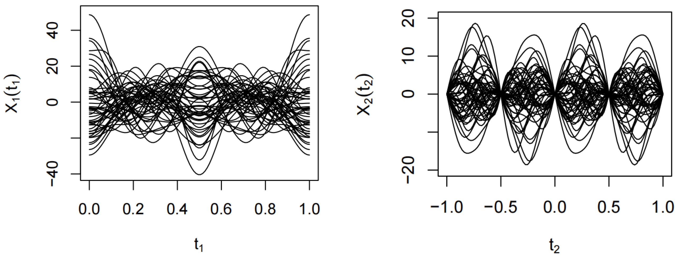
In this simulation, we consider the case that has two functional predictors, three scalar predictors, an interaction term between the two functional predictors, and a binary response. In order to include the case in which the functional predictors do not have the same domain, we define the functional predictors $X_{i1}\left(t_1\right),t_1\in [0,1]$ and $X_{i2}\left(t_2\right),t_2\in [-1,1]$, $i=1,\dots ,n,$ where n can be any positive integer. In the latter sample size, n takes the values of 50, 100, and 500, and, for each n, we run 100 simulations. First, we define two standard orthogonal bases ${\phi }_{1k}\left(t_1\right),t_1\in [0,1]$ and ${\phi }_{2l}\left(t_2\right),t_2\in [-1,1]$, satisfying

$${\phi }_{1k}\left(t_1\right)=\sqrt{2}cos\left(2k\pi t_1\right),k=1,\dots ,4,$$

$${\phi }_{2l}\left(t_2\right)=\sqrt{2}sin\left(2l\pi t_2\right),l=1,\dots ,5.$$

Under the Gaussian assumption, we define the two randomly generated functional principal component scores ${\chi }_{i1k},{\chi }_{i2l}$ that satisfy

$${\chi }_{i1k}\sim N(0,{\lambda }_{1k}),k=1,\dots ,4,$$

$${\chi }_{i2l}\sim N(0,{\lambda }_{2l}),l=1,\dots ,5,$$

where ${\lambda }_{11}=8,{\lambda }_{12}=6,{\lambda }_{13}=4,{\lambda }_{14}=2,$ ${\lambda }_{21}=4,{\lambda }_{22}=2,{\lambda }_{23}=1,{\lambda }_{24}={\displaystyle \frac{1}{2}},{\lambda }_{25}={\displaystyle \frac{1}{4}}$. Notice that the first three functional principal components explain up to 90% of the variation in the two predictors. So, we have

$$X_{i1}\left(t_1\right)=\sum _{k=1}^4{\chi }_{i1k}{\phi }_{1k}\left(t_1\right),$$

$$X_{i2}\left(t_2\right)=\sum _{l=1}^5{\chi }_{i2l}{\phi }_{2l}\left(t_2\right).$$

Fifty images of $X_1\left(t_1\right)$ and $X_2\left(t_2\right)$ are shown in Figure 1.

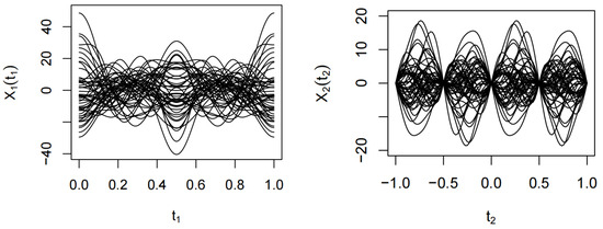
Figure 1. Functional predictors $X_1\left(t_1\right)$ and $X_2\left(t_2\right)$.

For scalar predictors, we assume $Z_1\sim N(0,2),$ $Z_2\sim N(0,5)$, and $Z_3\sim N(0,6).$

We assume that the theoretical values of the regression coefficients are

$$\gamma ={(4,6,8)}^T,$$

$${\beta }_1\left(t_1\right)=\sum _{k=1}^4{b}_{1k}{\phi }_{1k}\left(t_1\right),$$

$${\beta }_2\left(t_2\right)=\sum _{l=1}^5{b}_{2l}{\phi }_{2l}\left(t_2\right),$$

where $b_{1k}={\displaystyle \frac{k}{5}}$, $b_{2l}={\displaystyle \frac{l^2}{25}}.$

For the interaction term, its principal component score is denoted by ${\rho }_{ikl}$ and satisfies

$${\rho }_{ikl}={\chi }_{i1k}{\chi }_{i2l},$$

$${\psi }_{kl}(t_1,t_2)={\phi }_{1k}\left(t_1\right){\phi }_{2l}\left(t_2\right),$$

$$\beta (t_1,t_2)=\sum _{k=1}^4\sum _{l=1}^5{u}_{kl}{\phi }_{1k}\left(t_1\right){\phi }_{2l}\left(t_2\right),$$

where $u_{kl}={\left(\frac{k}{10}\right)}^2.$

The corresponding response variable is generated by

$$\begin{array}{cc}\hfill p(X_i,Z_i)=& g\left({\int }_{T_1}{X}_{i1}\left(t_1\right){\beta }_1\left(t_1\right)d{t}_1+{\int }_{T_2}{X}_{i2}\left(t_2\right){\beta }_2\left(t_2\right)d{t}_2\right.\hfill \\ & \left.+{\int \int }_{T_1\times T_2}{X}_{i1}\left(t_1\right)X_{i2}\left(t_2\right)\beta \left(t_1,t_2\right)d{t}_{1}d{t}_2+Z_i^T\gamma \right),\hfill \end{array}$$

where the link function $g\left(x\right)={\displaystyle \frac{exp\left(x\right)}{1+exp\left(x\right)}}$ and $Y(X,Z)\sim Bernoulli\left(p\right(X,Z\left)\right)$ is a sequence of pseudo-random numbers.

The principal component analysis was performed for $n=50,100,500$, and the running results showed that the principal component scores of $X_1$ with $90\%$ cumulative contribution were 3, 3, 3 for each sample size, respectively and the principal component scores of $X_2$ with $90\%$ cumulative contribution were 2, 2, 2.

Table 1 shows how the standardized prediction error (SPE) varies with different sample sizes, and the results show that the model’s predictions become more and more accurate as the sample size increases. Here, SPE is defined by ${\sum }_i|{\widehat{Y}}_i-Y_i|/{\sum }_i\left|Y_i\right|$.

Table 1. Standardized prediction error for different sample sizes.

n	SPE
50	0.0156
100	0.0130
500	0.0106

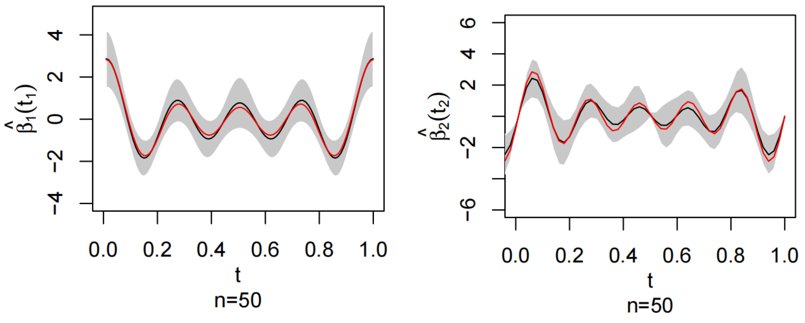
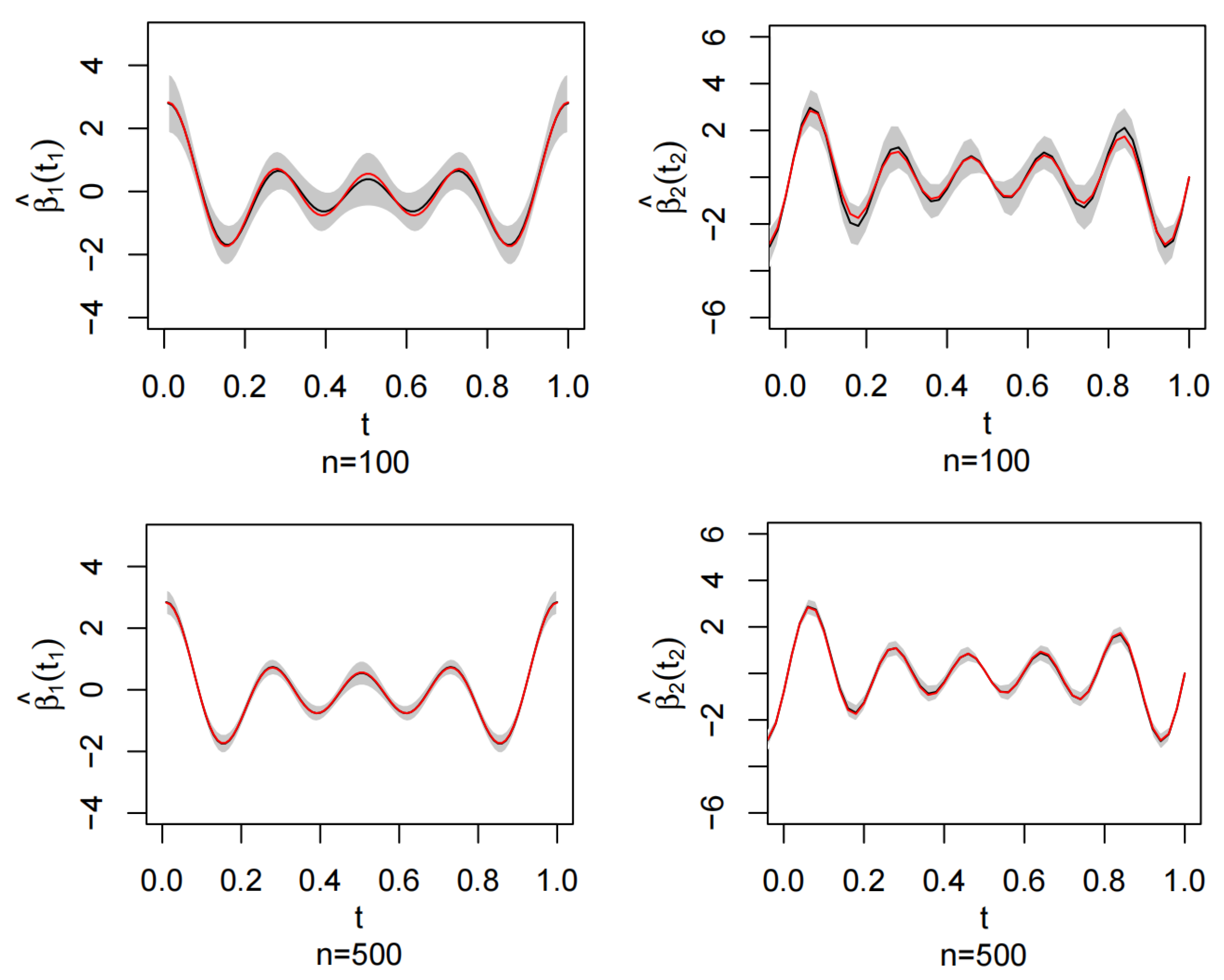
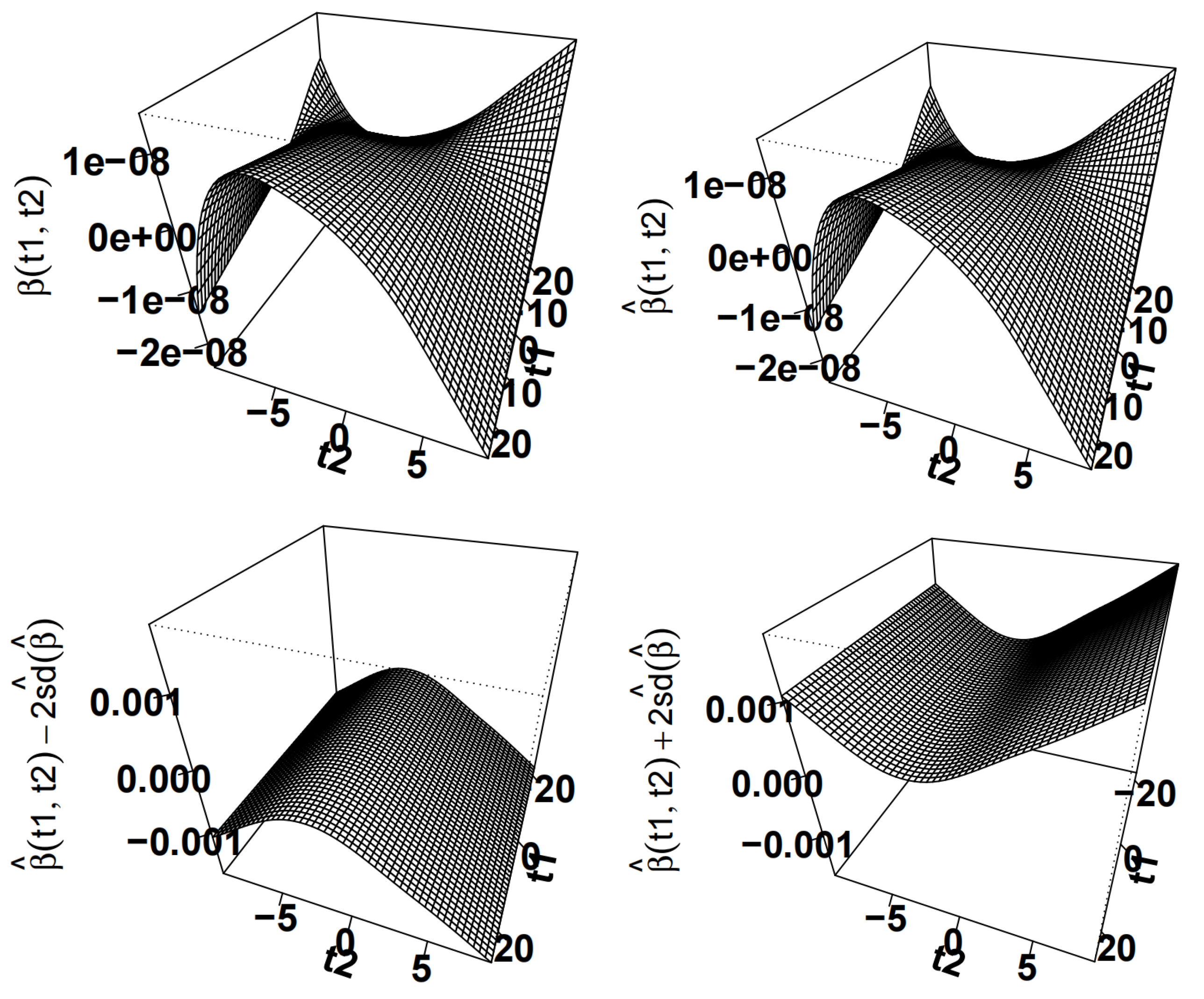
Figure 2 shows ${\widehat{\beta }}_1\left(t_1\right)$, ${\widehat{\beta }}_2\left(t_2\right)$ and the corresponding $95\%$ confidence interval bands for different sample sizes, where the red curves are the theoretical values of ${\beta }_1\left(t_1\right)$ and ${\beta }_2\left(t_2\right)$ and the black curves are the corresponding estimates ${\widehat{\beta }}_1\left(t_1\right)$ and ${\widehat{\beta }}_2\left(t_2\right).$ From Figure 2, it can be seen that, as the sample size increases, the estimated value becomes closer to the theoretical value. Figure 3 $\widehat{\beta }(t_1,t_2)$ shows the visualized 3D plot with $\widehat{\beta }(t_1,t_2)$ in the middle panel and the $95\%$ confidence intervals for $\widehat{\beta }(t_1,t_2)$ in the left and right panels.

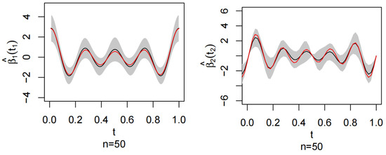
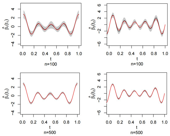
Figure 2. Estimated regression coefficient functions ${\widehat{\beta }}_1\left(t_1\right)$, ${\widehat{\beta }}_2\left(t_2\right)$ (black curves) and their $95\%$ confidence bands (grey area) for different sample sizes, where the red curves are the theoretical regression coefficient functions ${\beta }_1\left(t_1\right)$, ${\beta }_2\left(t_2\right)$.

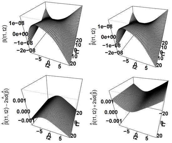
Figure 3. $\beta (t_1,t_2)$ and $\widehat{\beta }(t_1,t_2)$ are visualized in 3D.

Table 2 shows the estimated values of $\widehat{\gamma }$ and their corresponding standard deviations for different sample sizes. It can be seen that, as n increases, the standard deviation becomes smaller and the estimated value of $\gamma$ becomes closer to the theoretical value, where the theoretical values of $\gamma$ are 4, 6, and 8, respectively. Table 3 shows the standard deviation and root mean square error for ${\widehat{\beta }}_1,$ ${\widehat{\beta }}_2$ and $\widehat{\beta }(t_1,t_2)$ for different sample sizes. Here, we use the coefficients of the basis expansion of the regression coefficient function to calculate the root mean square error. For example, the root mean square error of ${\widehat{\beta }}_1$ is $\sqrt{{\sum }_{k=1}^4{({\widehat{b}}_{1k}-b_{1k})}^2}$. The results show that, as n increases, both the standard deviation and the RMS error become smaller, indicating that, as sample size increases, the prediction becomes more accurate.

Table 2. Estimates of the regression coefficients and their standard deviations.

n	${\widehat{\mathit{\gamma }}}_1$	${\widehat{\mathit{\gamma }}}_2$	${\widehat{\mathit{\gamma }}}_3$
50	3.912 (0.193)	5.902 (0.068)	8.053 (0.045)
100	4.013 (0.062)	5.958 (0.026)	8.015 (0.018)
500	3.998 (0.022)	5.993 (0.006)	7.996 (0.007)

Table 3. Standard deviation and root mean square error of the estimated values of the regression coefficient function.

	n	Sd	RMSE
${\widehat{\beta }}_1$	50	0.034	0.026
	100	0.018	0.006
	500	0.008	0.001
${\widehat{\beta }}_2$	50	0.325	0.204
	100	0.126	0.044
	500	0.043	0.004
$\widehat{\beta }(t_1,t_2)$	50	0.137	0.094
	100	0.054	0.024
	500	0.020	0.004

5. Application

To investigate the influence of the influence of air qualities, climate factors, medical and social indicators, and their interactions on cancer incidence using the proposed model, we collected data on average daily PM2.5 concentration, average daily humidity, per capita GDP, green coverage rate in built-up areas, the proportion of medical personnel (PMP), and the incidence of cancer in 49 cities in China from http://www.cnemc.cn/, http://www.stats.gov.cn/sj/ndsj/, and http://www.chinancpcn.org.cn/home.

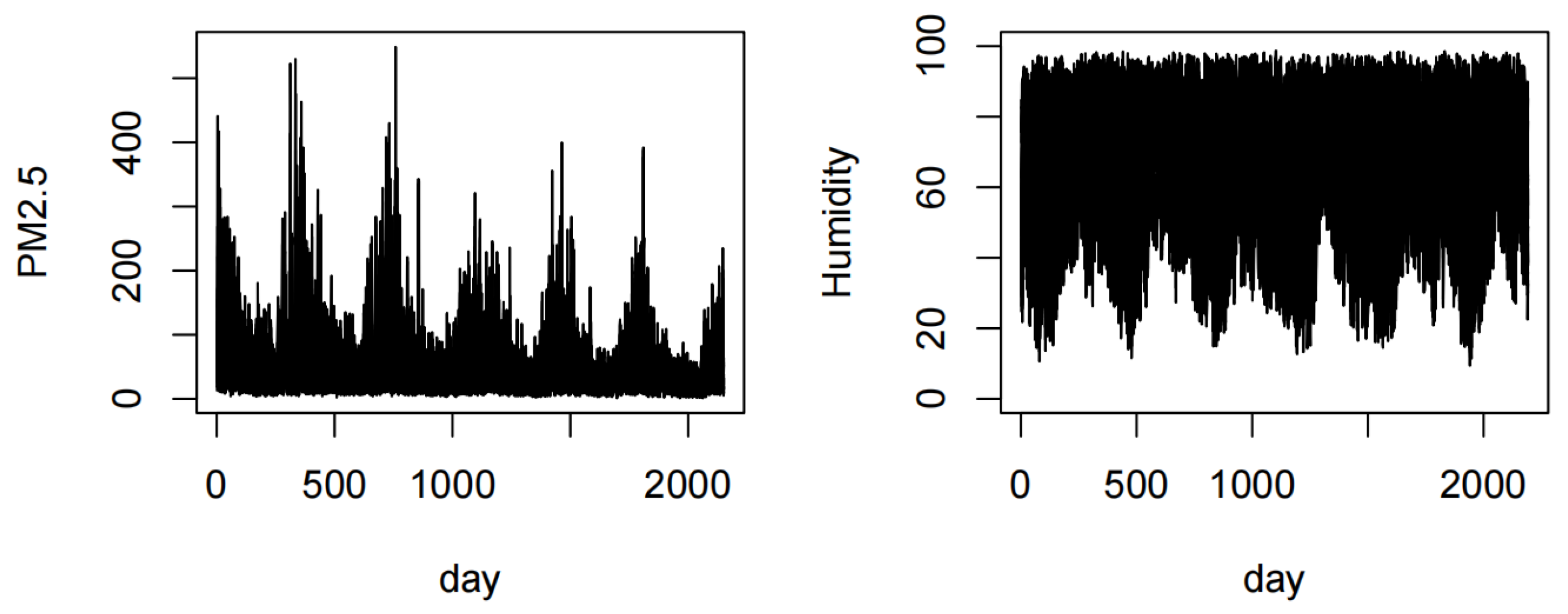
There are two functional predictors (average daily PM2.5 concentration and average daily humidity from 1 January 2015 to 31 December 2020), three scalar predictors (per capita GDP, greenery coverage, and PMP in 2020), and the response is the cancer incidence in 2020. The ratio of the number of new cancer cases to the total number of people in China in 2020 is $0.3156\%$. The data of the cancer incidence can only contain 0 and 1, indicating high or low cancer incidence rate. When the cancer incidence of a city was less than $0.3156\%$, the city was considered to have a low cancer incidence rate, denoted by 0; otherwise, the cancer incidence was high, denoted by 1. Figure 4 shows average daily PM2.5 concentration and daily relative humidity in 21 cities selected from the 49 cities.

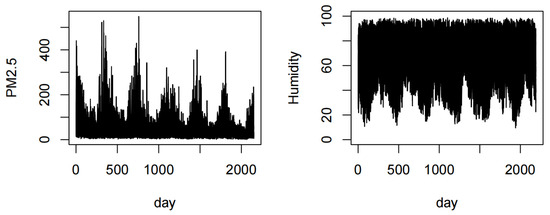
Figure 4. PM2.5 concentrations and average daily humidity in 21 selected cities in 2020.

We chose $g\left(x\right)={\displaystyle \frac{exp\left(x\right)}{1+exp\left(x\right)}}$ as the link function. The model was first subjected to principal component analysis and then the number of principal components was determined based on the cumulative contribution to obtain the number of functional principal components for PM2.5 concentrations and relative humidity, which were chosen as $p_{PM2.5}=7$, $p_{\mathrm{Humidity}}=14$ in order to explain 75% of the variation.

The prediction accuracy is shown by the Generalized Cross Validation (GCV) with a value of 0.0038.

The results of the regression coefficients for the scalar predictor variable $\widehat{\gamma }$ are shown in Table 4, where we can see that the per capita GDP is positively correlated with the incidence of cancer, i.e., the higher the GDP per capita, the higher the incidence of cancer in that city, which is consistent with the findings of Cao et al. [27]. The reason for this situation is that the promotion of cancer screening, early diagnosis, and treatment in the more economically developed regions has, to some extent, facilitated the detection of the disease. The greenery coverage is negatively correlated with the cancer incidence, i.e., the higher the greenery coverage, the lower the cancer incidence, which is also consistent with the findings of Wu et al. [26]. A high green coverage rate implies better air quality, which in turn reduces the risk of cancer. Additionally, a high green coverage rate may provide more outdoor recreational spaces, promoting physical activity and exercise, contributing to maintaining good physical health, and, thus, reducing the risk of cancer. The PMP is positively correlated with the incidence of cancer. As we all know, cancer incidence is age-related, and older people are more susceptible to cancer. The higher PMP, the better the medical conditions, the longer the average life expectancy of the people, and, therefore, the higher the cancer incidence.

Table 4. Estimates of regression coefficients and their levels of significance.

	Estimate	Std. Error	t Value	Pr (>|t|)
GDP	1.165 × 10−6	2.632 × 10−7	4.424	6.45 × 10−5 ***
Greenery coverage	−2.062 × 10−1	1.920 × 10−1	−2.654	0.0378 *
PMP	3.676 × 10−4	1.642 × 10−4	2.239	0.0491 *

PMP—Proportion of medical personnel. * indicates that the result is significant at the 5% significance level. *** indicates that the result is significant at the 0.1% significance level.

The regression coefficient functions ${\widehat{\beta }}_1\left(t_1\right)$ and ${\widehat{\beta }}_2\left(t_2\right)$ for the functional predictors are shown in Figure 5. From Figure 5, we can see that the effect of PM2.5 concentration on cancer incidence is generally positively correlated, i.e., the higher the PM2.5 concentration, the higher the cancer incidence. This result is consistent with Qin et al. [25] from 2014. Regarding the effect of humidity on cancer incidence, there is a more significant positive correlation between humidity and cancer incidence, i.e., the higher the humidity, the higher the cancer incidence. In high-humidity environments, there may be a higher presence of mold and fungi, and the spores and harmful substances released by these microorganisms may have negative effects on human health, increasing the risk of cancer. In high-humidity environments, pollutants in the air are more likely to adhere to suspended particles, making them more easily inhalable by humans. These pollutants include PM2.5, organic compounds, and heavy metals, which are believed to be associated with the occurrence of cancer. High humidity increases the survival time of bacteria and viruses in the air, increasing the chances of people becoming infected with diseases. Certain viruses such as hepatitis B virus and human papillomavirus (HPV) are believed to be associated with the occurrence of cancer.

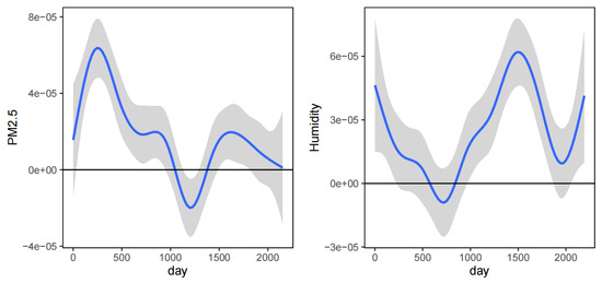
Figure 5. Regression coefficient functions ${\widehat{\beta }}_1\left(t_1\right)$, ${\widehat{\beta }}_2\left(t_2\right)$ and their $95\%$ confidence bands.

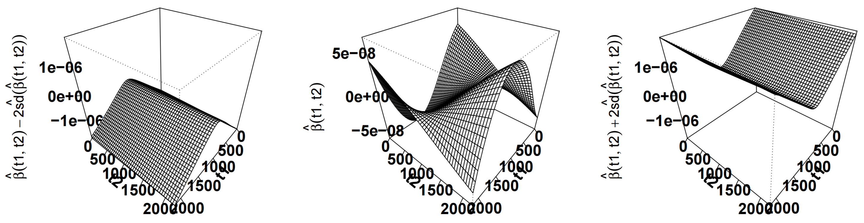
The interaction surface estimate $\widehat{\beta }(t_1,t_2)$ (middle) ± two times the estimated standard errors (left and right) are given in Figure 6. Figure 7 shows the contour map of $\widehat{\beta }(t_1,t_2)$, from which it can be seen that $\widehat{\beta }(t_1,t_2)$ decreases and then increases with $t_1$ when $t_2\in [0,1100]$ and increases and then decreases with $t_1$ when $t_2\in [1100,2192]$. In the conditions of higher humidity, PM2.5 particles may be more prone to settling, reducing the suspended harmful particles in the air, potentially lowering the incidence of cancer. Conversely, in lower-humidity conditions, PM2.5 may be more likely to remain suspended in the air, increasing the risk of respiratory system exposure, thereby raising the incidence of cancer. Additionally, the concentrations of PM2.5 and humidity may not fluctuate synchronously throughout the day. By introducing interaction terms, the model can capture the temporal complexities, making the estimation results more in line with real-world conditions.

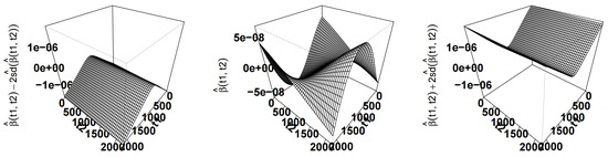
Figure 6. Visualization of $\widehat{\beta }(t_1,t_2)$ in 3D.

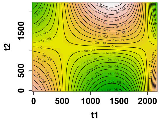
Figure 7. Contour map of $\widehat{\beta }(t_1,t_2)$.

To verify the necessity of considering the interaction term, i.e., to demonstrate the effectiveness of our proposed method, we compare mod1 proposed in this paper with mod2, which does not include the interaction term, i.e.,

$$\begin{array}{cc}\hfill mod1:Y_i=& g\left(\alpha +{\int }_{T_1}{X}_{i1}\left(t_1\right){\beta }_1\left(t_1\right)d{t}_1+{\int }_{T_2}{X}_{i2}\left(t_2\right){\beta }_2\left(t_2\right)d{t}_2\right.\hfill \\ \hfill & \left.+{\int \int }_{T_1\times T_2}{X}_{i1}\left(t_1\right)X_{i2}\left(t_2\right)\beta \left(t_1,t_2\right)d{t}_{1}d{t}_2+Z_i^T\gamma \right)+{\epsilon }_i.\hfill \end{array}$$

$$mod2:Y_i=g\left(\alpha +{\int }_{T_1}{X}_{i1}\left(t_1\right){\beta }_1\left(t_1\right)d{t}_1+{\int }_{T_2}{X}_{i2}\left(t_2\right){\beta }_2\left(t_2\right)d{t}_2+Z_i^T\gamma \right)+{\epsilon }_i.$$

The general standards for evaluating model performance are AIC (Akaike Information Criterion), residual, R-squared, RMSE (root mean square error), and MAE (mean absolute error). The smaller values of AIC, residuals, RMSE, and MAE indicate that the model’s fitting effect and generalization ability are better. The R-squared takes a value between 0 and 1, and, the bigger the value, the better the model’s fitting effect. According to Table 5, we can see that the AIC, residuals, RMSE, and MAE values of mod1 are smaller and that R-squared is much closer to 1 compared to that of mod2, which indicates that mod1 has a better performance. Thus, including the interaction term between PM2.5 concentration and relative humidity makes the research results more meaningful.

Table 5. Results of model comparison.

	AIC	R-Squared	Residual	RMSE	MAE
mod1	8.281	0.9287	0.7816	0.1263	0.1036
mod2	35.592	0.6465	3.2158	0.2562	0.1989

6. Discussion

This paper proposes a generalized partially functional linear model with interaction terms. We first use principal component analysis to reduce the dimensionality of the functional data, followed by maximum likelihood estimation to obtain the estimates of the unknown parameters, then prove the asymptotic property of the estimators, and finally perform data simulations and apply our model to a real data example.

As the incidence and mortality of cancer in China are increasing year by year, it is necessary to study the influencing factors and formulate corresponding measures. The effect of PM2.5 concentration, average daily humidity, per capita GDP, the greenery coverage of built-up areas, and PMP on cancer incidence in 49 cities in China was investigated, which showed that the effect of PM2.5 concentration and relative humidity on cancer incidence was generally positively correlated. The effect of greenery coverage in built-up areas on cancer incidence is negatively correlated, while the effect of per capita GDP and the proportion of medical personnel on cancer incidence is positively correlated. The higher the economic level and the more developed the medical conditions, the longer the average life expectancy of people and, therefore, the higher the cancer incidence. Comparing this model with the model without the interaction term shows that considering the role of the interaction term leads to more accurate and meaningful predictions.

Our research lays a foundation for further study on the generalized partially functional linear model with interaction terms and of unknown link function or variance function.

References

- Ramsay, J.O.; Silverman, B.W. Functional Data Analysis, 2nd ed.; Springer: New York, NY, USA, 2005. [Google Scholar]
- Horváth, L.; Kokoszka, P. Inference for Functional Data with Application; Springer: New York, NY, USA, 2012. [Google Scholar]
- Hsing, T.; Eubank, R. Theoretical Foundations of Functional Data Analysis, with an Introduction to Linear Operators; Springer: New York, NY, USA, 2015. [Google Scholar]
- Cardot, H.; Ferraty, F.; Sarda, P. Functional linear model. Stat. Probab. Lett. 1999, 45, 11–22. [Google Scholar] [CrossRef]
- Tony, C.; Peter, H. Prediction in functional linear regression. Ann. Stat. 2006, 34, 2159–2179. [Google Scholar] [CrossRef]
- Cardot, H.; Crambes, C.; Kneip, A.; Sarda, P. Smoothing Splines Estimators in Functional Linear Regression with Errors in Variables. Comput. Stat. Data Anal. 2007, 51, 4832–4848. [Google Scholar] [CrossRef]
- Delaigle, A.; Hall, P. Methodology and theory for partial least squares applied to functional data. Ann. Stat. 2012, 40, 322–352. [Google Scholar] [CrossRef]
- Cai, T.; Yuan, M. Minimax and adaptive prediction for functional linear regression. J. Am. Stat. Assoc. 2012, 107, 1201–1216. [Google Scholar] [CrossRef]
- Nelder, J.A.; Wedderburn, R.W.M. Generalized Linear Models. J. R. Stat. Soc. 1972, 135, 370–384. [Google Scholar] [CrossRef]
- James, G.M. Generalized linear models with functional predictors. J. R. Stat. Soc. Ser. B 2002, 64, 411–432. [Google Scholar] [CrossRef]
- Müller, H.G.; Stadtmüller, U. Generalized functional linear models. Ann. Stat. 2005, 33, 774–805. [Google Scholar] [CrossRef]
- Goldsmith, J.; Bobb, J.; Crainiceanu, C.M.; Caffo, B.; Reich, D. Penalized Functional Regression. J. Comput. Graph. Stat. 2011, 20, 830–851. [Google Scholar] [CrossRef]
- Xiao, W.W.; Wang, Y.X.; Liu, H.Y. Generalized partially functional linear model. Sci. Rep. 2021, 11, 23428. [Google Scholar] [CrossRef]
- Kong, D.; Xue, K.; Yao, F.; Zhang, H.H. Partially functional linear regression in high dimensions. Biometrika 2016, 103, 147–159. [Google Scholar] [CrossRef]
- Yao, F.; Sue, C.S.; Wang, F. Regularized partially functional quantile regression. J. Multivar. Anal. 2017, 156, 39–56. [Google Scholar] [CrossRef]
- Ma, H.; Li, T.; Zhu, H.; Zhu, Z. Quantile regression for functional partially linear model in ultra-high dimensions. Comput. Stat. Data Anal. 2019, 129, 135–147. [Google Scholar] [CrossRef]
- Xu, W.; Ding, H.; Zhang, R.; Liang, H. Estimation and inference in partially functional linear regression with multiple functional covariates. J. Stat. Plan. Inference 2020, 209, 44–61. [Google Scholar] [CrossRef]
- Usset, J.; Staicu, A.M.; Maity, A. Interaction models for functional regression. Comput. Stat. Data Anal. 2016, 94, 317–329. [Google Scholar] [CrossRef]
- Luo, R.; Qi, X. Interaction Model and Model Selection for Function-on-Function Regression. J. Comput. Graph. Stat. 2019, 28, 309–322. [Google Scholar] [CrossRef]
- Yang, W.H.; Wikle, C.K.; Holan, S.H.; Wildhaber, M.L. Ecological Prediction with Nonlinear Multivariate Time-Frequency Functional Data Models. J. Agric. Biol. Environ. Stat. 2013, 18, 450–474. [Google Scholar] [CrossRef]
- Matsui, H. Quadratic regression for functional response models. Econom. Stat. 2020, 13, 125–136. [Google Scholar] [CrossRef]
- Sun, Y.; Wang, Q. Function-on-function quadratic regression models. Comput. Stat. Data Anal. 2020, 142, 106814. [Google Scholar] [CrossRef]
- Fuchs, K.; Scheipl, F.; Greven, S. Penalized scalar-on-functions regression with interaction term. Comput. Stat. Data Anal. 2015, 81, 38–51. [Google Scholar] [CrossRef]
- Qiu, H.; Cao, S.; Xu, R. Cancer incidence, mortality, and burden in China: A time-trend analysis and comparison with the United States and United Kingdom based on the global epidemiological data released in 2020. Cancer Commun. 2021, 41, 1037–1048. [Google Scholar] [CrossRef]
- Qin, X.; Wan, F.; Zhang, H.; Dai, B.; Shi, G.; Zhu, Y.; Ye, D. Relationship between air pollution PM2.5 concentration and cancer. In Proceedings of the 8th Chinese Oncology Academic Conference and the 13th Cross-Strait Oncology Academic Conference, Jinan, China, 12–13 September 2014; p. 76. [Google Scholar]
- Wu, X.; Feng, Y.; Chang, K.; Jia, X.; Xue, F. Analysis of the causal relationship between green coverage and the incidence of cancer. J. Shandong Univ. (Health Sci.) 2022, 60, 115–119. [Google Scholar]
- Cao, W.; Li, F.; Liang, Y.; Yu, D. Analysis of the relationship between the level of economic development and cancer incidence and mortality in selected regions of China. Chin. J. Dis. Control Prev. 2023, 27, 209–215. [Google Scholar] [CrossRef]
- Xu, J.; Kuang, H.Y.; Wang, G.Q.; Chen, M.; Lu, L. Analysis of the relationship between PM2.5 and air relative humidity. Agric. Technol. 2017, 37, 148–149. [Google Scholar]
- Yang, Z.; Wang, Y.K.; Xu, X.H.; Yang, J.; Ou, C.Q. Quantifying and characterizing the impacts of PM2.5 and humidity on atmospheric visibility in 182 Chinese cities: A nationwide time-series study. J. Clean. Prod. 2022, 368, 133182. [Google Scholar] [CrossRef]
Disclaimer/Publisher’s Note: The statements, opinions and data contained in all publications are solely those of the individual author(s) and contributor(s) and not of MDPI and/or the editor(s). MDPI and/or the editor(s) disclaim responsibility for any injury to people or property resulting from any ideas, methods, instructions or products referred to in the content. |
© 2024 by the authors. Licensee MDPI, Basel, Switzerland. This article is an open access article distributed under the terms and conditions of the Creative Commons Attribution (CC BY) license (https://creativecommons.org/licenses/by/4.0/).