Stability and Convergence Analysis of the Discrete Dynamical System for Simulating a Moving Bed

Abstract

The efficiency of controlling the simulated moving bed (SMB) has long been a critical issue in the chemical engineering industry. Most existing research relies on finite element methods, which often result in lower control efficiency and are unable to achieve online control. To enhance control over the SMB process, this paper employs the Crank–Nicolson method to develop a discrete dynamical model. This approach allows for the investigation of system stability and convergence, fundamentally addressing the sources of error. During the discretization of partial differential equations (PDEs), two main types of errors arise: intrinsic errors from the method itself and truncation errors due to derivative approximations and the discretization process. Research indicates that for the former, the iterative process remains convergent as long as the time and spatial steps are sufficiently small. Regarding truncation errors, studies have demonstrated that they exhibit second-order behavior relative to time and spatial steps. The theoretical validation shows that the iteration works effectively, and simulations confirm that the finite difference method is stable and performs well with varying SMB system parameters and controller processes. This provides a solid theoretical foundation for practical, real-time online control.

1. Introduction

Simulated moving bed (SMB) technology is a sophisticated process employed for the separation and purification of chemical materials or mixtures. It operates on the principle of a moving bed, leveraging the dynamic flow characteristics of materials within the bed to achieve separation. Typically, SMB technology comprises a fixed bed alongside a system that mimics the behavior of a moving bed. By simulating the fluid flow and material movement within the bed, this technology replicates the separation processes of an actual moving bed. The essence of SMB technology lies in its ability to separate various components by modulating the direction or speed of fluid flow. This technology finds extensive application in industries such as chemical engineering, petrochemicals, and pharmaceuticals [1,2,3]. The process of the SMB is illustrated in Figure 1. The advent of SMB technology has significantly improved separation efficiency within the chromatography industry. Nonetheless, due to the numerous parameters inherent in industrial processes, optimizing these parameters through empirical experimentation is both time-consuming and costly. Technicians often rely on their experience to set initial control parameters for the SMB, a practice that frequently results in suboptimal operation [4,5,6].

Researchers have been focusing on analyzing SMB processes using mathematical models. The main models used are the general rate model and the equilibrium diffusion model. The general rate model is very detailed and closely matches real processes, but it is complex. On the other hand, the equilibrium diffusion model is simpler and works well when the concentrations of substances being separated are low [7]. This model can be further divided into different types based on the isotherm used: linear, Langmuir, modified Langmuir, and competitive Langmuir isotherms [8].

Irrespective of the model employed, these models typically comprise a set of partial differential equations for which analytical solutions are challenging to derive. The ultimate objective of SMB technology is to achieve effective control, necessitating a focus on the efficiency of the solution process for these models. To this end, it is crucial to investigate the convergence and stability of the computational models for the SMB.

Dunnebier et al. proposed and compared three different modeling and simulation methods, evaluating the solutions in terms of complexity, accuracy, and computational time. The newly developed closed-form solution demonstrated high accuracy and low computational time [9]. Andrade Neto et al. presented a self-adjusting nonlinear MPC method for the enantiomeric separation of Praziquantel in an analog moving bed apparatus that was based on the finite element method [10]. Muhammed et al. developed a rigorous dynamic model to compare the SMB with traditional distillation as the next best choice [11]. The SMB was optimized using a genetic algorithm, maximizing the Research Octane Number (RON) and gross margin as the objective functions. Z. Yan et al. applied the finite difference method to establish a matrix subspace iteration method, conducting numerical simulations on parameters such as isotherm, mass transfer resistance, cycle switching time, number of series-connected columns, column type, length, diameter, volume, feed concentration, and circulation flow rate to build a column movement model. This work laid the foundation for the optimal control of the column [12]. Leao et al. proposed a numerical solution process for simulating the transient and steady-state behavior of the simulated moving bed (SMB) based on a mathematical model [13]. Majeed et al. investigated the accuracy and efficiency of using orthogonal collocation methods to solve partial differential equations in separation engineering, with the numerical solutions provided being almost as accurate as those obtained from actual machinery [14]. Y. Kim et al. performed computational fluid dynamics (CFD) simulations using the finite element method to obtain concentration data and conducted experimental analysis using residence time distribution to support their findings [15]. The model integrates diffusion mass transfer mechanisms and dual-substrate Monod kinetics. WS-Lee et al. employed a mathematical dynamic model with limited experimental parameters, alongside a data-driven machine learning approach using real industrial data, to evaluate the performance of the SMB [16].

In the field of controller research, SMB systems exhibit a diverse array of approaches, with various controllers being designed specifically for different materials to be separated. Wei et al. proposed a control method based on a piecewise affine model. The simulation results demonstrate the feasibility of this approach, as it can fit the actual yield–production curve of the target compound and impurities to achieve the desired target yield [17]. Hoon et al. applied a data-driven deep Q-network, a model-free reinforcement learning method, to train near-optimal control strategies for the SMB process [18]. Natarajan and Lee proposed applying Repetitive Model Predictive Control (RMPC) to the SMB process, specifically for the chromatographic separation of phenylalanine–tryptophan mixtures [19]. Klatt et al. introduced a model-based optimization control scheme for SMB chromatographic separation and its application in the separation of fructose and glucose [20]. Carlos and Alain introduced a novel method for controlling the SMB chromatographic separation process [21]. Marrocos et al. proposed a deep artificial intelligence structure for online soft measurement that incorporates a nonlinear output error (NOE) framework and a nonlinear autoregressive with an exogenous input (NARX) predictor. This structure provides key insights into the primary characteristics of simulated moving bed chromatography equipment [22]. Santos et al. have developed a theoretical model to describe the adsorption and desorption kinetics of succinic acid and water mixtures in commercial resin-fixed beds. This model has been utilized for the design and optimization of simulated moving bed control processes [23]. Suzuki et al. employed parameter estimation methods to estimate the system, validated the predictive capability of the resulting model using test datasets, and evaluated the confidence intervals of the parameters. These tests confirmed that the model shows improvement compared to the initially obtained model [24]. Other relevant studies can be referenced in [25,26,27].

Overall, past research can be categorized into two main aspects: the study of computational models for SMB systems and the research on controllers. Most computational models focus on the finite element method (FEM), as FEM theory is well established, and many controller designs are based on the FEM. However, this raises two significant issues. Although the FEM provides high accuracy, it suffers from low computational efficiency, leading to prolonged latency in controllers and affecting their performance. Moreover, FEM-based controllers cannot achieve real-time online control with existing hardware infrastructure. To address these issues, this study initially explores the application of the Crank–Nicolson discretization method in SMB systems, demonstrating that the finite difference method (FDM) is also feasible. Subsequent chapters of the study mathematically validate the convergence of iterative calculations and the order of errors. Experimental simulations are then conducted, adjusting parameters of the SMB system, including feed concentration, adsorbent parameters, and switching times, to verify the feasibility of the finite difference method. Finally, a PID controller is used to control the SMB purity based on the finite difference method, further confirming that controllers based on finite difference methods are also stable and reliable.

2. Discrete Model for SMB

2.1. Using Crank–Nicolson Method for Discrete Partial Differential Equations

The SMB model originates from the TMB model. The meanings of the parameters are shown in

Table 1. Parameters of SMB system.

Parameter	Nomenclature	Parameter	Nomenclature
$x (\mathrm{cm})$	Axial distance	$Q ({\mathrm{cm}}^3{\min }^{-1})$	Volume flow rate
$k ({\mathrm{gL}}^{-1})$	Comprehensive mass transfer constant	$t (\mathrm{s})$	Time
$v^{\ast } (\mathrm{cm}{\min }^{-1})$	Effect velocity of body	$D ({\mathrm{cm}}^2{\min }^{-1})$	Effective dispersion coefficient
$u_s (\mathrm{cm}{\min }^{-1})$	Solid flow rate	$\epsilon$	Bulk void fraction
$C ({\mathrm{gL}}^{-1})$	Mobile phase concentration	$i$	Material index: A or B
$q ({\mathrm{gL}}^{-1})$	Solid phase concentration	$j$	Column number: 1, 2, 3, 4, 5, 6, 7, 8
$q^{\ast } ({\mathrm{gL}}^{-1})$	Solid phase concentration at equilibrium between solid phase and mobile phase

below.

The relevant literature [10] provides a brief introduction to the transformation between the TMB model and the SMB model.

$${\displaystyle \frac{\partial C_{ij}}{\partial t}}=D_i {\displaystyle \frac{{\partial }^2{C}_{ij}}{\partial x^2}}-v_j^{TMB} {\displaystyle \frac{\partial C_{ij}}{\partial x}}-{\displaystyle \frac{1-\epsilon }{\epsilon }}{k}_i (q_{ij}^{\ast }-q_{ij})$$

(1)

$${\displaystyle \frac{\partial q_{ij}}{\partial t}}={\displaystyle \frac{\partial }{\partial x}} u_s q_{ij}+k_i (q_{ij}^{\ast }-q_{ij})$$

(2)

$v_j^{TMB}$ is the velocity of the TMB system. Therefore, based on the principle of kinematic synthesis, the formula for the conversion between velocities is expressed as Equation (3).

$$v_j^{SMB}=v_j^{TMB}+u_s$$

(3)

Since the solid phase is achieved through column switching controlled by switching time, the equivalent flow rate of the solid phase can be expressed by Equation (4).

$$u_s={\displaystyle \frac{L}{T_{\theta }}}$$

(4)

$L$ is the length of the column; the mathematical model of the SMB system can be obtained as:

$${\displaystyle \frac{\partial C_{ij}}{\partial t}}=D_i {\displaystyle \frac{{\partial }^2{C}_{ij}}{\partial x^2}}-v_j^{SMB} {\displaystyle \frac{\partial C_{ij}}{\partial x}}-{\displaystyle \frac{1-\epsilon }{\epsilon }}{k}_i (q_{ij}^{\ast }-q_{ij})$$

(5)

$${\displaystyle \frac{\partial q_{ij}}{\partial t}}=k_i (q_{ij}^{\ast }-q_{ij})$$

(6)

$v_j^{SMB}$ is denoted as $v_j^{\ast }$, and we can obtain Equation (7) by substituting Equation (6) into Equation (5).

$${\displaystyle \frac{\partial C_{ij}}{\partial t}}=D_i {\displaystyle \frac{{\partial }^2{C}_{ij}}{\partial x^2}}-v_j^{\ast } {\displaystyle \frac{\partial C_{ij}}{\partial x}}-{\displaystyle \frac{1-\epsilon }{\epsilon }} {\displaystyle \frac{\partial q_{ij}}{\partial t}}$$

(7)

In this study, the focus is mainly on the case of linear isotherms, as follows:

$$q_{ij}=H_i C_{ij}$$

(8)

Set

$$E={\displaystyle \frac{1-\epsilon }{\epsilon }}$$

(9)

Equation (7) can be rewritten by substituting Equations (8) and (9), shown as Equation (10).

$$(1+E{H}_i) {\displaystyle \frac{\partial C_{ij}}{\partial t}}=D_i {\displaystyle \frac{{\partial }^2{C}_{ij}}{\partial x^2}}-v_j^{\ast } {\displaystyle \frac{\partial C_{ij}}{\partial x}}$$

(10)

The Crank–Nicolson method employs central differencing for the spatial domain and utilizes the trapezoidal rule for the temporal domain, thereby achieving second-order convergence in time. For instance, for a one-dimensional partial differential equation,

$${\displaystyle \frac{\partial u}{\partial t}}=F(u,x,t,{\displaystyle \frac{\partial u}{\partial x}},{\displaystyle \frac{{\partial }^{2}u}{\partial x^2}})$$

(11)

Denote $\Delta x$ and $\Delta t$ as the spatial and temporal step sizes, respectively, and denote $u(i\Delta x,j\Delta t)=u_i^j$, then the Crank–Nicolson discretized formula is as follows [28]:

$${\displaystyle \frac{u_i^{j+1}-u_i^j}{\Delta t}}={\displaystyle \frac{1}{2}}(F_i^{j+1}(u,x,t,{\displaystyle \frac{\partial u}{\partial x}},{\displaystyle \frac{{\partial }^{2}u}{\partial x^2}})+F_i^j(u,x,t,{\displaystyle \frac{\partial u}{\partial x}},{\displaystyle \frac{{\partial }^{2}u}{\partial x^2}}))$$

(12)

Since the Crank–Nicolson method uses central difference formulas in the spatial domain, its formulas are expressed as follows:

$${\displaystyle \frac{{\partial }^{2}u}{\partial x^2}}{|}_i={\displaystyle \frac{u_{i+1}-2u_i+u_{i-1}}{\Delta x^2}}$$

(13)

$${\displaystyle \frac{\partial u}{\partial x}}{|}_i={\displaystyle \frac{u_{i+1}-u_{i-1}}{2\Delta x}}$$

(14)

Comparing Equations (10) and (11), it can be observed that

$$(1+E{H}_i){\displaystyle \frac{\partial C_{ij}}{\partial t}}=F(C_{ij},x,t,{\displaystyle \frac{\partial C_{ij}}{\partial x}},{\displaystyle \frac{{\partial }^2{C}_{ij}}{\partial x^2}})$$

(15)

$$F(C_{ij},x,t,{\displaystyle \frac{\partial C_{ij}}{\partial x}},{\displaystyle \frac{{\partial }^2{C}_{ij}}{\partial x^2}})=D_i{\displaystyle \frac{{\partial }^2{C}_{ij}}{\partial x^2}}-v_j^{\ast }{\displaystyle \frac{\partial C_{ij}}{\partial x}}$$

(16)

The form of Equation (16) now includes first-order partial derivatives in the spatial domain. Since indices $i,j$ have already been used to represent material types and column numbers, we chose $l,k$ as indices for the spatial and temporal domains, respectively. Therefore, the left-hand side of Equation (15) can be written as

$$(1+E{H}_i){\displaystyle \frac{C_{ij,l}^{k+1}-C_{ij,l}^k}{\Delta t}}$$

Hence, we can have the discretization formula for the right-hand side of Equation (16) as

$$\begin{array}{l}{\displaystyle \frac{1}{2}}(F_l^{k+1}(C_{ij},x,t,{\displaystyle \frac{\partial C_{ij}}{\partial x}},{\displaystyle \frac{{\partial }^2{C}_{ij}}{\partial x^2}})+F_l^k(C_{ij},x,t,{\displaystyle \frac{\partial C_{ij}}{\partial x}},{\displaystyle \frac{{\partial }^2{C}_{ij}}{\partial x^2}}))\\ ={\displaystyle \frac{1}{2}}{D}_i({\displaystyle \frac{{\partial }^2{C}_{ij}}{\partial x^2}}{|}_l^{k+1}+{\displaystyle \frac{{\partial }^2{C}_{ij}}{\partial x^2}}{|}_l^k)-{\displaystyle \frac{1}{2}}{v}_j^{\ast }({\displaystyle \frac{\partial C_{ij}}{\partial x}}{|}_l^{k+1}+{\displaystyle \frac{\partial C_{ij}}{\partial x}}{|}_l^k)\end{array}$$

(17)

According to Equations (13) and (14), we can obtain

$${\displaystyle \frac{1}{2}}{D}_i({\displaystyle \frac{{\partial }^2{C}_{ij}}{\partial x^2}}{|}_l^{k+1}+{\displaystyle \frac{{\partial }^2{C}_{ij}}{\partial x^2}}{|}_l^k)=D_i{\displaystyle \frac{((C_{ij,l-1}^{k+1}-2C_{ij,l}^{k+1}+C_{ij,l+1}^{k+1})+(C_{ij,l-1}^k-2C_{ij,l}^k+C_{ij,l+1}^k))}{2\Delta x^2}}$$

(18)

$${\displaystyle \frac{1}{2}}{v}_j^{\ast }({\displaystyle \frac{\partial C_{ij}}{\partial x}}{|}_l^{k+1}+{\displaystyle \frac{\partial C_{ij}}{\partial x}}{|}_l^k)=v_j^{\ast }{\displaystyle \frac{((C_{ij,l+1}^{k+1}-C_{ij,l-1}^{k+1})+(C_{ij,l+1}^k-C_{ij,l-1}^k))}{4\Delta x}}$$

(19)

By substituting Equations (18) and (19) into Equation (12), we obtain

$$\begin{array}{l}(1+E{H}_i){\displaystyle \frac{C_{ij,l}^{k+1}-C_{ij,l}^k}{\Delta t}}=D_i{\displaystyle \frac{((C_{ij,l-1}^{k+1}-2C_{ij,l}^{k+1}+C_{ij,l+1}^{k+1})+(C_{ij,l-1}^k-2C_{ij,l}^k+C_{ij,l+1}^k))}{2\Delta x^2}}-\\ v_j^{\ast }{\displaystyle \frac{((C_{ij,l+1}^{k+1}-C_{ij,l-1}^{k+1})+(C_{ij,l+1}^k-C_{ij,l-1}^k))}{4\Delta x}}\end{array}$$

(20)

According to Equation (20), move the terms at time point K + 1 to the left side of the equation and move the terms at time point K to the right side, resulting in the iterative computation Equation (21) as follows:

$$\begin{array}{l}(1+E{H}_i+{\displaystyle \frac{D_i\Delta t}{\Delta x^2}})C_{ij,l}^{k+1}-({\displaystyle \frac{v_j^{\ast }\Delta t}{4\Delta x}}+{\displaystyle \frac{D_i\Delta t}{2\Delta x^2}})C_{ij,l-1}^{k+1}+({\displaystyle \frac{v_j^{\ast }\Delta t}{4\Delta x}}-{\displaystyle \frac{D_i\Delta t}{2\Delta x^2}})C_{ij,l+1}^{k+1}\\ =({\displaystyle \frac{v_j^{\ast }\Delta t}{4\Delta x}}+{\displaystyle \frac{D_i\Delta t}{2\Delta x^2}})C_{ij,l-1}^k+(1+E{H}_i-{\displaystyle \frac{D_i\Delta t}{\Delta x^2}})C_{ij,l}^k+({\displaystyle \frac{D_i\Delta t}{2\Delta x^2}}-{\displaystyle \frac{v_j^{\ast }\Delta t}{4\Delta x}})C_{ij,l+1}^k\end{array}$$

(21)

2.2. Boundary Numerate Condition

With the boundary conditions:

Initial condition:

$$C_{ij}(x , 0)=C_{0ij}$$

(22)

Space conditions:

$${\displaystyle \frac{\partial C_{ij}(x,t)}{\partial x}}{|}_{x=L_{end}}=0$$

(23)

$$D_i{\displaystyle \frac{\partial C_{ij}(x,t)}{\partial x}}{|}_{x=L_0}=v_j^{\ast }[C_{ij}(L_0,t)-{\stackrel{-}{C}}_{ij}^{\sec t}(t)]$$

(24)

$C_{0ij}$ represents the initial concentration distribution at time = 0. The space boundaries are represented by $L_{end}$ and $L_0$, which are the conditions of the end and initial positions of the pipe column. The ${\stackrel{-}{C}}_{ij}^{\sec t}(t)$ term is related to the region in which it is located. Since Equation (24) describes the concentration changes at the pipe head, the head of each region depends on the flow rate at the inlet of that region, the material concentration, the concentration at the end of the previous column, and the flow rate of the region in contact with the inlet. Therefore, this term can be divided into three cases, as shown in the following formulas:

$${\stackrel{-}{C}}_{ij}^{\mathrm{I}}(t)={\displaystyle \frac{Q_{IV} C_{ij-1}(l_{n-1} , t)}{Q_I}},Zone I, 1^{st}column$$

(25)

$${\stackrel{-}{C}}_{ij}^{\mathrm{III}}(t)={\displaystyle \frac{Q_{II} C_{ij-1}(l_{n-1} , t)+Q_f C_{fi}}{Q_{III}}},Zone III,1^{st}column$$

(26)

$${\stackrel{-}{C}}_{ij}^{\sec t}(t)=C_{ij-1}(l_{n-1} , t),other$$

(27)

$C_{fi}$ is the concentration of the material in the imported column, and Q is the flow rate of each section.

Assuming that each column is divided into n + 1 components, Equation (23) can be obtained from Equation (12):

$$0={\displaystyle \frac{\partial C_{ij}(x,t)}{\partial x}}{|}_{x=L_{end}}={\displaystyle \frac{1}{2}}({\displaystyle \frac{\partial C_{ij}}{\partial x}}{|}_n^{k+1}+{\displaystyle \frac{\partial C_{ij}}{\partial x}}{|}_n^k)={\displaystyle \frac{((C_{ij,n+1}^{k+1}-C_{ij,n-1}^{k+1})+(C_{ij,n+1}^k-C_{ij,n-1}^k))}{4\Delta x}}$$

(28)

Through the separation of space points n + 1 and space point n − 1, we obtain

$$C_{ij,n+1}^k+C_{ij,n+1}^{k+1}=C_{ij,n-1}^k+C_{ij,n-1}^{k+1}$$

(29)

By setting the spatial point $j=n$ in Equation (21), we obtain

$$\begin{array}{l}(1+E{H}_i+{\displaystyle \frac{D_i\Delta t}{\Delta x^2}})C_{ij,n}^{k+1}-({\displaystyle \frac{v_j^{\ast }\Delta t}{4\Delta x}}+{\displaystyle \frac{D_i\Delta t}{2\Delta x^2}})C_{ij,n-1}^{k+1}+({\displaystyle \frac{v_j^{\ast }\Delta t}{4\Delta x}}-{\displaystyle \frac{D_i\Delta t}{2\Delta x^2}})C_{ij,n+1}^{k+1}\\ =({\displaystyle \frac{v_j^{\ast }\Delta t}{4\Delta x}}+{\displaystyle \frac{D_i\Delta t}{2\Delta x^2}})C_{ij,n-1}^k+(1+E{H}_i-{\displaystyle \frac{D_i\Delta t}{\Delta x^2}})C_{ij,n}^k+({\displaystyle \frac{D_i\Delta t}{2\Delta x^2}}-{\displaystyle \frac{v_j^{\ast }\Delta t}{4\Delta x}})C_{ij,n+1}^k\end{array}$$

(30)

Substituting Equation (29) into Equation (30), the following equation can be obtained:

$$\begin{array}{l}(1+E{H}_i+{\displaystyle \frac{D_i\Delta t}{\Delta x^2}})C_{ij,n}^{k+1}-({\displaystyle \frac{v_j^{\ast }\Delta t}{4\Delta x}}+{\displaystyle \frac{D_i\Delta t}{2\Delta x^2}})C_{ij,n-1}^{k+1}+({\displaystyle \frac{v_j^{\ast }\Delta t}{4\Delta x}}-{\displaystyle \frac{D_i\Delta t}{2\Delta x^2}})C_{ij,n-1}^{k+1}\\ =({\displaystyle \frac{v_j^{\ast }\Delta t}{4\Delta x}}+{\displaystyle \frac{D_i\Delta t}{2\Delta x^2}})C_{ij,n-1}^k+(1+E{H}_i-{\displaystyle \frac{D_i\Delta t}{\Delta x^2}})C_{ij,n}^k+({\displaystyle \frac{D_i\Delta t}{2\Delta x^2}}-{\displaystyle \frac{v_j^{\ast }\Delta t}{4\Delta x}})C_{ij,n-1}^k\end{array}$$

(31)

Merging similar items, we obtain

$$-{\displaystyle \frac{D_i\Delta t}{\Delta x^2}}{C}_{ij,n-1}^{k+1}+(1+E{H}_i+{\displaystyle \frac{D_i\Delta t}{\Delta x^2}})C_{ij,n}^{k+1}={\displaystyle \frac{D_i\Delta t}{\Delta x^2}}{C}_{ij,n-1}^k+(1+E{H}_i-{\displaystyle \frac{D_i\Delta t}{\Delta x^2}})C_{ij,n}^k$$

(32)

Equation (33) can be obtained from Equation (24).

$$\begin{array}{l}{\displaystyle \frac{v_j^{\ast }}{D_i}}[C_{ij,1}^k-{\stackrel{-}{C}}_{ij}^{\sec t}(k)]={\displaystyle \frac{\partial C_{ij}(x,t)}{\partial x}}{|}_{x=L_0}={\displaystyle \frac{1}{2}}({\displaystyle \frac{\partial C_{ij}}{\partial x}}{|}_1^{k+1}+{\displaystyle \frac{\partial C_{ij}}{\partial x}}{|}_1^k)=\\ {\displaystyle \frac{((C_{ij,2}^{k+1}-C_{ij,0}^{k+1})+(C_{ij,2}^k-C_{ij,0}^k))}{4h}}\end{array}$$

(33)

Through the separation of space point 0 and space points 1 and 2, we obtain

$$C_{ij,2}^{k+1}+C_{ij,2}^k-{\displaystyle \frac{4h{v}_j^{\ast }}{D_i}}(C_{ij,1}^k-{\stackrel{-}{C}}_{ij}^{\sec t}(k))=C_{ij,0}^{k+1}+C_{ij,0}^k$$

(34)

By setting the spatial point $j=1$ in Equation (21), it can be obtained that

$$\begin{array}{l}(1+F{H}_i+{\displaystyle \frac{D_{i}s}{h^2}})C_{ij,1}^{k+1}-({\displaystyle \frac{v_j^{\ast }s}{4h}}+{\displaystyle \frac{D_{i}s}{2h^2}})C_{ij,0}^{k+1}+({\displaystyle \frac{v_j^{\ast }s}{4h}}-{\displaystyle \frac{D_{i}s}{2h^2}})C_{ij,2}^{k+1}\\ =({\displaystyle \frac{v_j^{\ast }s}{4h}}+{\displaystyle \frac{D_{i}s}{2h^2}})C_{ij,0}^k+(1+F{H}_i-{\displaystyle \frac{D_{i}s}{h^2}})C_{ij,1}^k+({\displaystyle \frac{D_{i}s}{2h^2}}-{\displaystyle \frac{v_j^{\ast }s}{4h}})C_{ij,2}^k\end{array}$$

(35)

Substituting Equation (34) into Equation (35), we obtain the following equation:

$$\begin{array}{l}(1+E{H}_i+{\displaystyle \frac{D_i\Delta t}{\Delta x^2}})C_{ij,1}^{k+1}+({\displaystyle \frac{v_j^{\ast }\Delta t}{4\Delta x}}-{\displaystyle \frac{D_i\Delta t}{2\Delta x^2}})C_{ij,2}^{k+1}-({\displaystyle \frac{v_j^{\ast }\Delta t}{4\Delta x}}+{\displaystyle \frac{D_i\Delta t}{2\Delta x^2}})C_{ij,2}^{k+1}=\\ -({\displaystyle \frac{v_j^{\ast }\Delta t}{4\Delta x}}+{\displaystyle \frac{D_i\Delta t}{2\Delta x^2}}){\displaystyle \frac{4\Delta x{v}_j^{\ast }}{D_i}}(C_{ij,1}^k-{\stackrel{-}{C}}_{ij}^{\sec t}(k))+(1+E{H}_i-{\displaystyle \frac{D_i\Delta t}{\Delta x^2}})C_{ij,1}^k+\\ ({\displaystyle \frac{D_i\Delta t}{2\Delta x^2}}-{\displaystyle \frac{v_j^{\ast }\Delta t}{4\Delta x}})C_{ij,2}^k+({\displaystyle \frac{v_j^{\ast }\Delta t}{4\Delta x}}+{\displaystyle \frac{D_i\Delta t}{2\Delta x^2}})C_{ij,2}^{k+1}\end{array}$$

(36)

Again, merging similar items can lead to

$$\begin{array}{l}(1+E{H}_i+{\displaystyle \frac{D_i\Delta t}{\Delta x^2}})C_{ij,1}^{k+1}-{\displaystyle \frac{D_i\Delta t}{\Delta x^2}}{C}_{ij,2}^{k+1}=({\displaystyle \frac{v_j^{\ast 2}\Delta t}{D_i}}+{\displaystyle \frac{2v_j^{\ast }\Delta t}{\Delta x}}){\stackrel{-}{C}}_{ij}^{\sec t}(k)+\\ (1+E{H}_i-{\displaystyle \frac{D_i\Delta t}{\Delta x^2}}-{\displaystyle \frac{v_j^{\ast 2}\Delta t}{D_i}}-{\displaystyle \frac{2v_j^{\ast }\Delta t}{\Delta x}})C_{ij,1}^k+{\displaystyle \frac{D_i\Delta t}{\Delta x^2}}{C}_{ij,2}^k\end{array}$$

(37)

To simplify symbols, we set

$$m={\displaystyle \frac{v_j^{\ast }\Delta t}{4\Delta x}}$$

(38)

$$p={\displaystyle \frac{D_i\Delta t}{2\Delta x^2}}$$

(39)

Then

$$v_j^{\ast }={\displaystyle \frac{4m\Delta x}{\Delta t}}$$

(40)

$$D_i={\displaystyle \frac{2\Delta x^{2}p}{\Delta t}}$$

(41)

Substituting Equations (40) and (41) into Equation (37) yields

$$\begin{array}{l}(1+E{H}_i+2p)C_{ij,1}^{k+1}-2p{C}_{ij,2}^{k+1}=({\displaystyle \frac{16m^2\Delta x^2}{\Delta t^2}}{\displaystyle \frac{\Delta t\Delta t}{2\Delta x^{2}p}}+{\displaystyle \frac{8m\Delta x\Delta t}{\Delta t\Delta x}}){\stackrel{-}{C}}_{ij}^{\sec t}(k)+\\ (1+E{H}_i-2p-{\displaystyle \frac{16m^2\Delta x^2}{\Delta t^2}}{\displaystyle \frac{\Delta t\Delta t}{2\Delta x^{2}p}}-{\displaystyle \frac{8m\Delta x\Delta t}{\Delta t\Delta x}})C_{ij,1}^k+2p{C}_{ij,2}^k\end{array}$$

(42)

Simplify Equation (42) as follows:

$$\begin{array}{l}(1+E{H}_i+2p)C_{ij,1}^{k+1}-2p{C}_{ij,2}^{k+1}={\displaystyle \frac{8m(m+p)}{p}}{\stackrel{-}{C}}_{ij}^{\sec t}(k)+\\ (1+E{H}_i-2p-{\displaystyle \frac{8m(m+p)}{p}})C_{ij,1}^k+2p{C}_{ij,2}^k\end{array}$$

(43)

Substituting Equations (40) and (41) into Equation (21) yields the middle position of a spatial point equation as follows:

$$\begin{array}{l}(1+E{H}_i+2p)C_{ij,l}^{k+1}-(m+p)C_{ij,l-1}^{k+1}+(m-p)C_{ij,l+1}^{k+1}\\ =(m+p)C_{ij,l-1}^k+(1+E{H}_i-2p)C_{ij,l}^k+(p-m)C_{ij,l+1}^k\end{array}$$

(44)

Substituting Equations (40) and (41) into Equation (32) yields the end position of a spatial point equation.

$$-2p{C}_{ij,n-1}^{k+1}+(1+E{H}_i+2p)C_{ij,n}^{k+1}=2p{C}_{ij,n-1}^k+(1+E{H}_i-2p)C_{ij,n}^k$$

(45)

According to Equations (43)–(45), (44), we denote the matric

$$A={\left[\begin{array}{ccccc}1+E{H}_i+2p& -2p& 0& \cdots & 0\\ -(m+p)& 1+E{H}_i+2p& (m-p)& \cdots & 0\\ ⋮& ⋮& ⋮& ⋮& ⋮\\ 0& \cdots & -(m+p)& 1+E{H}_i+2p& (m-p)\\ 0& \cdots & 0& -2p& 1+E{H}_i+2p\end{array}\right]}_{n\times n}$$

(46)

$$B={\left[\begin{array}{ccccc}1+E{H}_i-2p-{\displaystyle \frac{8m(m+p)}{p}}& 2p& 0& \cdots & 0\\ (m+p)& 1+E{H}_i-2p& -(m-p)& \cdots & 0\\ ⋮& ⋮& ⋮& ⋮& ⋮\\ 0& \cdots & (m+p)& 1+E{H}_i-2p& -(m-p)\\ 0& \cdots & 0& 2p& 1+E{H}_i-2p\end{array}\right]}_{n\times n}$$

(47)

Set

$$C_{ij}^k={[C_{ij,1}^k,C_{ij,2}^k,\cdots ,C_{ij,n}^k]}_{ 1\times n}^T$$

(48)

$$w(k)={\left(\begin{array}{ccccc}{\displaystyle \frac{8m(m+p)}{p}}{\stackrel{-}{C}}_{ij}^{\sec t}(k)& 0& \cdots & 0& 0\end{array}\right)}_{{ }^{1\times n}}^T$$

(49)

From Equations (43)–(45), the final iteration equation can be unified into the following matrix equation.

$$A{C}_{ij}^{k+1}=B{C}_{ij}^k+w(k)$$

(50)

3. Stability and Convergence Analysis

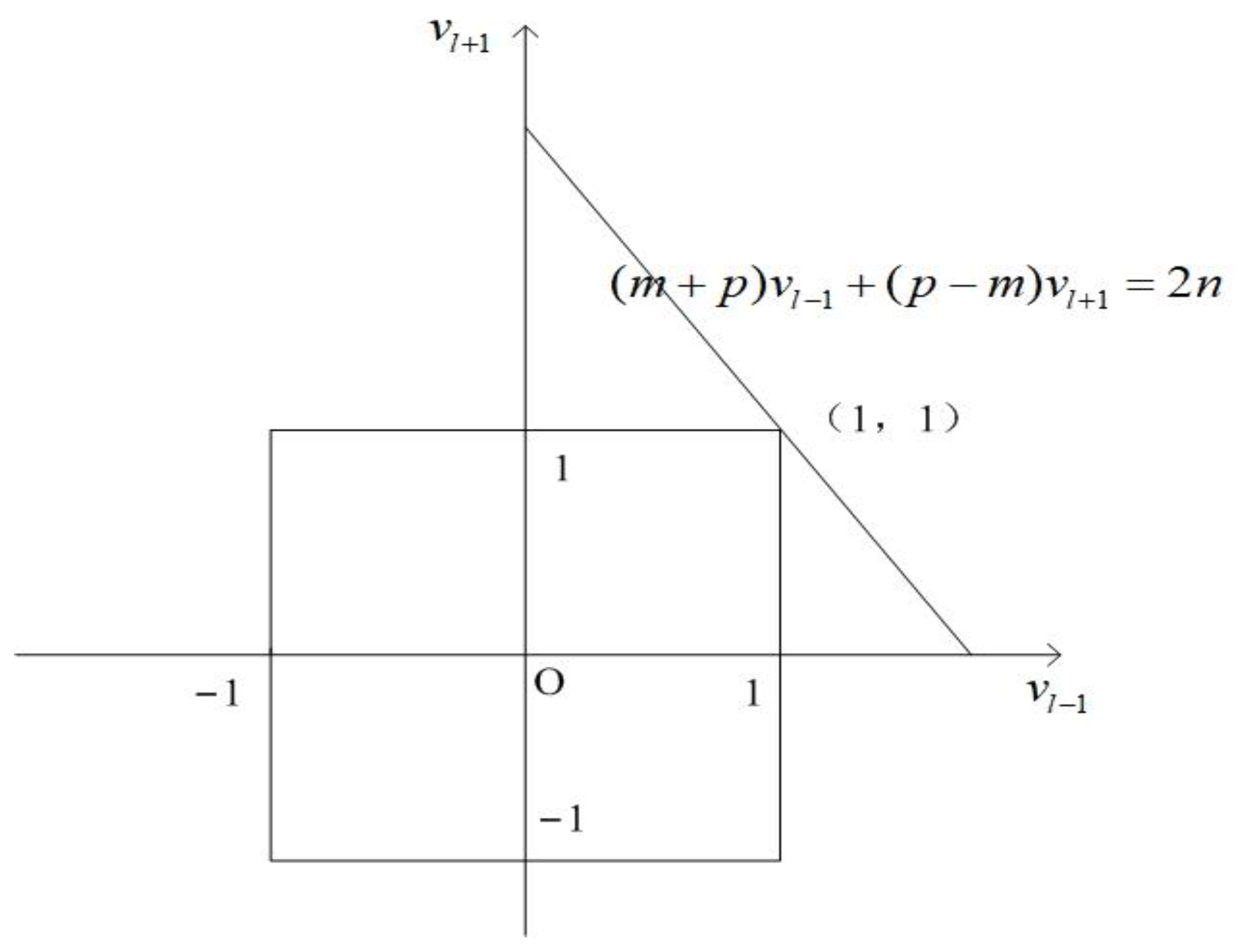
3.1. Stability Analysis

When discussing the stability of the Crank–Nicolson method applied to SMB systems, it is crucial to consider the sources of error in the discretization process of partial differential equations (PDEs). Typically, errors fall into two categories: truncation errors due to the discretization of derivative approximations and inherent error amplification of the numerical method itself. To estimate truncation errors, the Taylor error formula can be employed, which provides an estimate of the errors introduced by discretizing derivatives. To explore whether errors are amplified or dampened, it is necessary to closely examine the behavior of the finite difference method. Von Neumann stability analysis is commonly used to assess whether errors are amplified in numerical methods. For the SMB discretization process, this method’s stability requires selecting an appropriate step size or time increment to ensure that the amplification factor measured by the Von Neumann stability analysis does not exceed 1. By carefully considering truncation errors and employing an appropriate step size in Von Neumann stability analysis, we can evaluate the stability of the Crank–Nicolson method when applied to SMB systems.

Set $C_{ij}^{\ast }(k)$ is the exact solution of Equation (50), and set $y_{ij}(k)$ is the approximate solution obtained by calculation and satisfying $A{y}_{ij}(k+1)=B{y}_{ij}(k)+w(k)$. The difference between them is $e_{ij}(k)=y_{ij}(k)-C_{ij}^{\ast }(k)$, and it is satisfied that

$$\begin{array}{l}A{e}_{ij}(k)=A{y}_{ij}(k)-A{C}_{ij}^{\ast }(k)=B{y}_{ij}(k-1)+w(k-1)-(B{C}_{ij}^{\ast }(k-1)+w(k-1))\\ =B{e}_{ij}(k-1)\end{array}$$

(51)

If A is nonsingular, we can obtain

$$e_{ij}(k)=A^{-1}B{e}_{ij}(k-1)$$

(52)

The spectral radius of $A^{-1}B$ must satisfy $\rho (A^{-1}B)<1$ to ensure the error $e_{ij}(k)$ is not amplified.

Theorem 1. 

If matrix A is strictly diagonally dominant and it satisfies $|a_{ii}|>{\displaystyle \sum _{\begin{array}{l}j=1\\ j\ne i\end{array}}^n|a_{ij}|}$, (i =1, 2, …, n), then matrix A is nonsingular.

Proof. 

If matrix A is a singular matrix, then there is a non-zero vector x that satisfies $Ax=0$. Set $|x_1|=\max \{|x_1|,|x_2|\cdots |x_n|\}$, $so |x_1|\ne 0$, so it can obtain

$$a_{11}{x}_1+a_{12}{x}_2+\cdots a_{1n}{x}_n=0,a_{11}=-a_{12}{\displaystyle \frac{x_2}{x_1}}-\cdots a_{1n}{\displaystyle \frac{x_n}{x_1}}$$

(53)

$$|a_{11}|\le |a_{12}||{\displaystyle \frac{x_2}{x_1}}|+\cdots |a_{1n}||{\displaystyle \frac{x_n}{x_1}}|\le {\displaystyle \sum _{j=2}^n{a}_{1j}}$$

(54)

This contradicts the condition, so matrix A is nonsingular. □

Set $m={\displaystyle \frac{v_j^{\ast }\Delta t}{4\Delta x}}=O(s),p={\displaystyle \frac{D_i\Delta t}{2\Delta x^2}}=O(s)$ represents an infinitesimal of the same order. As long as the time step is sufficiently small, matrices A and B exhibit strict diagonal dominance, making them non-singular. Therefore, we can use the Crank–Nicolson method to establish the stability of the iterative process involved in computing the SMB system. By ensuring that the time step is sufficiently small, the strict diagonal dominance of matrices A and B guarantees their non-singularity, thereby enhancing the stability of the iterative process used in the Crank–Nicolson method for computing the SMB system.

Theorem 2. 

If the space step ($\Delta x$) and time step ($\Delta t$) are both sufficiently small, $A{C}_{ij}(k+1)=B{C}_{ij}(k)+w(k)$ is stable.

Proof. 

Hypothesis $\lambda$ is the eigenvalue of $A^{-1}B$, and $v$ is the corresponding eigenvector. Select $||v|{|}_{\infty }=1$, and the dimension of Matrix A is $n\times n$. So with $|v_k|\le 1,1\le k\le n$, choose component index $v_l=1$. Indicators are divided into three situations:

(1) $2\le l\le n-1$. Accordingly, $A^{-1}Bv=\lambda v\Rightarrow Bv=\lambda Av$, so we can get in component $l$:

$$\begin{array}{l}(m+p)v_{l-1}+(1+EH-2p)v_l+(p-m)v_{l+1}=\lambda [-(m+p)v_{l-1}+\\ (1+EH+2p)v_l+(m-p)v_{l+1}]\end{array}$$

(55)

$$\mathrm{If} |\lambda |={\displaystyle \frac{|(m+p)v_{l-1}+(1+EH-2p)+(p-m)v_{l+1}|}{|[-(m+p)v_{l-1}+(1+EH+2p)+(m-p)v_{l+1}]|}}<1$$

(56)

As $m={\displaystyle \frac{v_j^{\ast }\Delta t}{4\Delta x}}=O(s),p={\displaystyle \frac{D_i\Delta t}{2\Delta x^2}}=O(s),$ so

$$\forall \epsilon >0,\exists \delta ,when \Delta t<\delta (\Delta x),we \mathrm{obtain}|m|\le \epsilon ,|p|\le \epsilon$$

For any $\Delta t$, select a space step $\Delta x$ that is small enough to have $p>m\Rightarrow \Delta x<{\displaystyle \frac{D}{v^{\ast }}}$.

So, we obtain

$$(m+p)v_{l-1}+(p-m)v_{l+1}<2n$$

(57)

For the split line over the fixed point (1, 1)

$$(m+p)v_{l-1}+(p-m)v_{l+1}=2n$$

(58)

Rectangle $(v_{l-1},v_{l+1})\in [-1,1]\times [-1,1]$ (Figure 2) is under the split line, so it satisfies the inequality (57) except $(1,1)$ shown in Figure 2. Therefore, $|\lambda |\le 1$ can be inferred.

Equality is established only if $v_{l-1}=1,v_{l+1}=1$.

Now, it has been proven that if the components of the eigenvector satisfy this condition, then a contradiction will arise with the previous component.

$$\begin{array}{l}(m+p)v_{l-2}+(1+EH-2p)v_{l-1}+(p-m)v_l=[-(m+p)v_{l-2}+\\ (1+EH-2p)v_{l-1}+(m-p)v_l]\end{array}$$

(59)

Simplify Equation (59), and we obtain $v_{l-2}=1$.

Any component can be achieved by the same principle $v_k=1,k=1,\cdots n$.

However, for the first component equation

$$(1+EH-2p-{\displaystyle \frac{8m(m+p)}{p}})+2p=(1+EH+2p)-2p\Rightarrow {\displaystyle \frac{8m(m+p)}{p}}=0$$

as $m={\displaystyle \frac{v_j^{\ast }\Delta t}{4\Delta x}}>0,p={\displaystyle \frac{D_i\Delta t}{2\Delta x^2}}>0$, so ${\displaystyle \frac{8m(m+p)}{p}}>0$. The statement contradicts the previous equation ${\displaystyle \frac{8m(m+p)}{p}}=0$.

Thus, $|\lambda |<1$.

(2) $l=1$, which means

$$(1+EH-2p-{\displaystyle \frac{8m(m+p)}{p}})+2p{v}_2=\lambda [(1+EH+2p)-2p{v}_2]\Rightarrow$$

(60)

$$\mathrm{If} |\lambda |={\displaystyle \frac{(1+EH-2p-\frac{8m(m+p)}{p})+2p{v}_2}{(1+EH+2p)-2p{v}_2}}<1$$

(61)

$$v_2<1+{\displaystyle \frac{2m(m+p)}{p^2}}$$

(62)

As $||v|{|}_{\infty }=1$, so $|\lambda |<1$.

(3) $l=n$, which means

$$1+EH-2p+2p{v}_{n-1}=\lambda [(1+EH+2p)-2p{v}_{n-1}]\Rightarrow$$

(63)

$$\mathrm{If} |\lambda |={\displaystyle \frac{1+EH-2p+2p{v}_{n-1}}{[(1+EH+2p)-2p{v}_{n-1}]}}<1$$

(64)

$$v_{n-1}<1$$

(65)

When $v_{n-1}=1\Rightarrow$$\lambda =1$.

It has been proven that if the components of the feature vector are in this situation, contradictions will occur.

$$\begin{array}{l}(m+p)v_{l-2}+(1+EH-2p)v_{l-1}+(p-m)v_l=[-(m+p)v_{l-2}+\\ (1+EH-2p)v_{l-1}+(m-p)v_l]\end{array}$$

(66)

Like the first case, any component can be obtained by the same principle $v_k=1,k=1,\cdots n$. So $|\lambda |<1$ and be proved. □

3.2. Convergence Analysis

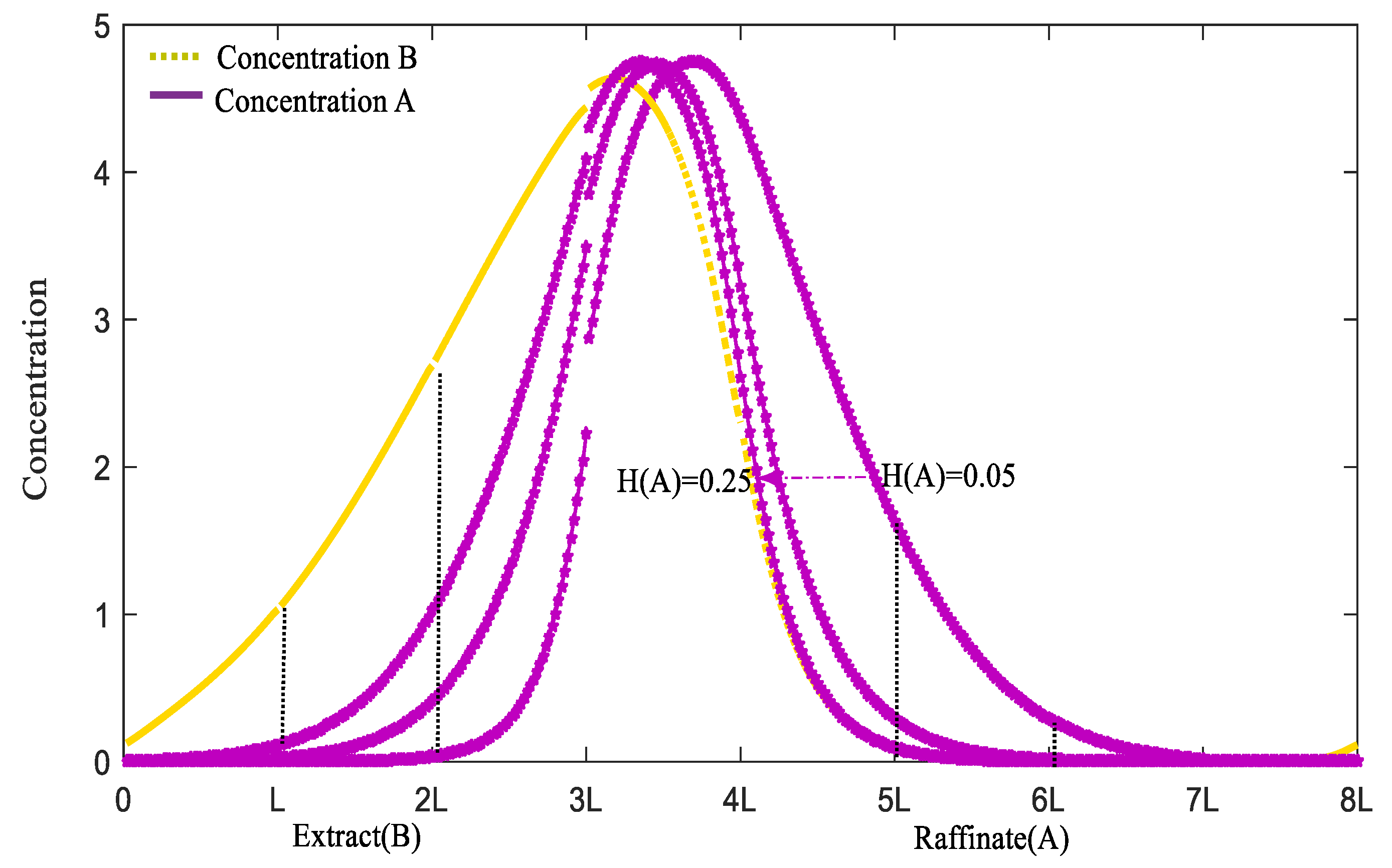
Denote

$$\begin{array}{l}{\displaystyle \frac{\partial C_{ij}}{\partial x}}=C_x,{\displaystyle \frac{{\partial }^2{C}_{ij}}{\partial x^2}}=C_{xx},,{\displaystyle \frac{{\partial }^3{C}_{ij}}{\partial x^3}}=C_{xxx},,{\displaystyle \frac{{\partial }^4{C}_{ij}}{\partial x^4}}=C_{xxxx},{\displaystyle \frac{\partial C_{ij}}{\partial t}}=C_t,{\displaystyle \frac{{\partial }^2{C}_{ij}}{\partial t^2}}=C_{tt}\\ {\displaystyle \frac{{\partial }^3{C}_{ij}}{\partial t^3}}=C_{ttt},{\displaystyle \frac{{\partial }^2{C}_{ij}}{\partial x\partial t}}=C_{xt},{\displaystyle \frac{{\partial }^3{C}_{ij}}{\partial x^2\partial t}}=C_{xxt},{\displaystyle \frac{{\partial }^3{C}_{ij}}{\partial x\partial t^2}}=C_{xtt},{\displaystyle \frac{{\partial }^4{C}_{ij}}{\partial x^2\partial t^2}}=C_{xxtt}\end{array},$$

and $C(l,k)$ represents the concentration at position $l$ in space at time $k$.

Theorem 3. 

The truncation error of SMB discrete dynamical systems is the sum of the squares of the time step size and the spatial step size: $O(s^2)+O(h^2)$.

Proof: 

Using the backward difference formula,

$$C_t(l,k)={\displaystyle \frac{C(l,k)-C(l,k-1)}{s}}+{\displaystyle \frac{1}{2}}s{C}_{tt}(l,k)-{\displaystyle \frac{1}{6}}{s}^2{C}_{ttt}(l,k_1),k_1\in (k-1,k)s$$

(67)

$s$ represents the time step. According to the Taylor series expansion formula,

$$C_{xx}(l,k-1)=C_{xx}(l,k)-s{C}_{xxt}(l,k)-{\displaystyle \frac{1}{2}}{s}^2{C}_{xxtt}(l,k_2),k_2\in (k-1,k)s$$

(68)

$$C_{xx}(l,k)=C_{xx}(l,k-1)+s{C}_{xxt}(l,k)+{\displaystyle \frac{1}{2}}{s}^2{C}_{xxtt}(l,k_2),k_2\in (k-1,k)s$$

(69)

By the central difference formula of the second derivative, $h$ represents the spatial step, and the following equations can be obtained.

$$C_{xx}(l,k)={\displaystyle \frac{C(l-1,k)-2C(l,k)+C(l+1,k)}{h^2}}+{\displaystyle \frac{h^2}{12}}{C}_{xxxx}(l_1,k)$$

(70)

$$C_{xx}(l,k-1)={\displaystyle \frac{C(l-1,k-1)-2C(l,k-1)+C(l+1,k-1)}{h^2}}+{\displaystyle \frac{h^2}{12}}{C}_{xxxx}(l_2,k-1)$$

(71)

$$l_1,l_2\in (l-1,l)h$$

According to the central difference formula for the first derivative,

$$C_x(l,k)={\displaystyle \frac{C(l+1,k)-C(l-1,k)}{2h}}-{\displaystyle \frac{h^2}{12}}[C_{xxx}(l_3,k)+C_{xxx}(l_4,k)]$$

(72)

$$C_x(l,k-1)={\displaystyle \frac{C(l+1,k-1)-C(l-1,k-1)}{2h}}-{\displaystyle \frac{h^2}{12}}[C_{xxx}(l_5,k-1)+C_{xxx}(l_6,k-1)]$$

(73)

$$l_3,l_4,l_5,l_6\in (l-1,l)s$$

For the first-order partial derivative ${\displaystyle \frac{\partial C_{ij}}{\partial x}}$, by taking the Taylor series expansion,

$$C_x(l,k)=C_x(l,k-1)+s{C}_{xt}(l,k)+{\displaystyle \frac{1}{2}}{s}^2{C}_{xtt}(l,k_3),k_3\in (k-1,k)s$$

(74)

The SMB system equation is as follows:

$$(1+EH){\displaystyle \frac{\partial C}{\partial t}}=D{\displaystyle \frac{{\partial }^{2}C}{\partial x^2}}-v{\displaystyle \frac{\partial C}{\partial x}}$$

(75)

Substituting Equations (67)–(74) into Equation (75), Equation (76) can be obtained as follows:

$$\begin{array}{l}(1+EH)[{\displaystyle \frac{C(l,k)-C(l,k-1)}{s}}+{\displaystyle \frac{1}{2}}s{C}_{tt}(l,k)-{\displaystyle \frac{1}{6}}{s}^2{C}_{ttt}(l,k_1)]=\\ {\displaystyle \frac{1}{2}}D[{\displaystyle \frac{C(l-1,k)-2C(l,k)+C(l+1,k)}{h^2}}+{\displaystyle \frac{h^2}{12}}{C}_{xxxx}(l_1,k)]+\\ {\displaystyle \frac{1}{2}}D[s{C}_{xxt}(l,k)+{\displaystyle \frac{1}{2}}{s}^2{C}_{xxtt}(l,k_2)]+\\ {\displaystyle \frac{1}{2}}D[{\displaystyle \frac{C(l-1,k-1)-2C(l,k-1)+C(l+1,k-1)}{h^2}}+{\displaystyle \frac{h^2}{12}}{C}_{xxxx}(l_2,k-1)]\\ -{\displaystyle \frac{1}{2}}{v}^{\ast }[{\displaystyle \frac{C(l+1,k)-C(l+1,k)}{2h}}-{\displaystyle \frac{h^2}{12}}(C_{xxx}(l_3,k)+C_{xxx}(l_4,k))]-\\ {\displaystyle \frac{1}{2}}{v}^{\ast }[s{C}_{xt}(l,k)+{\displaystyle \frac{1}{2}}{s}^2{C}_{xtt}(l,k_3)+{\displaystyle \frac{C(l-1,k-1)-C(l+1,k-1)}{2h}}-\\ {\displaystyle \frac{h^2}{12}}(C_{xxx}(l_5,k-1)+C_{xxx}(l_6,k-1))]\end{array}$$

(76)

Moving the terms in Equation (76) gives the following Equation (77).

$$\begin{array}{l}(1+EH){\displaystyle \frac{C(l,k)-C(l,k-1)}{s}}-{\displaystyle \frac{1}{2}}D{\displaystyle \frac{C(l-1,k)-2C(l,k)+C(l+1,k)}{h^2}}-\\ {\displaystyle \frac{1}{2}}D{\displaystyle \frac{C(l-1,k-1)-2C(l,k-1)+C(l+1,k-1)}{h^2}}+{\displaystyle \frac{1}{2}}{v}^{\ast }{\displaystyle \frac{C(l+1,k)-C(l+1,k)}{2h}}+\\ {\displaystyle \frac{1}{2}}{v}^{\ast }{\displaystyle \frac{C(l-1,k-1)-C(l+1,k-1)}{2h}}=-{\displaystyle \frac{1}{2}}(1+EH)s{C}_{tt}(l,k)+{\displaystyle \frac{1}{6}}(1+EH)s^2{C}_{ttt}(l,k_1)+\\ {\displaystyle \frac{h^2}{24}}D[C_{xxxx}(l_1,k)+C_{xxxx}(l_2,k-1)]+{\displaystyle \frac{1}{2}}Ds{C}_{xxt}(l,k)+{\displaystyle \frac{1}{4}}D{s}^2{C}_{xxtt}(l,k_2)+{\displaystyle \frac{v^{\ast }{h}^2}{24}}[C_{xxx}(l_3,k)\\ +C_{xxx}(l_4,k)+C_{xxx}(l_5,k-1)+C_{xxx}(l_6,k-1)]-{\displaystyle \frac{1}{2}}{v}^{\ast }[s{C}_{xt}(l,k)+{\displaystyle \frac{1}{2}}{s}^2{C}_{xtt}(l,k_3)]\end{array}$$

(77)

In Equation (77), the left side represents the result of the discretization of the SMB system, while the right side contains the residual error terms involving the time step size $s$ and spatial step size $h$. By rearranging the right side of Equation (77), the following expression, Equation (78), can be obtained.

$$\begin{array}{l}-{\displaystyle \frac{1}{2}}(1+EH)s{C}_{tt}(l,k)+{\displaystyle \frac{1}{6}}(1+EH)s^2{C}_{ttt}(l,k_1)+{\displaystyle \frac{h^2}{24}}D[C_{xxxx}(l_1,k)+C_{xxxx}(l_2,k-1)]+{\displaystyle \frac{1}{2}}Ds{C}_{xxt}(l,k)+\\ {\displaystyle \frac{1}{4}}D{s}^2{C}_{xxtt}(l,k_2)+{\displaystyle \frac{v{h}^2}{12}}[C_{xxx}(l_3,k)+C_{xxx}(l_4,k-1)]-{\displaystyle \frac{1}{2}}v[s{C}_{xt}(l,k)+{\displaystyle \frac{1}{2}}{s}^2{C}_{xtt}(l,k_3)]=\\ =[-{\displaystyle \frac{1}{2}}(1+EH)s{C}_{tt}(l,k)+{\displaystyle \frac{1}{2}}Ds{C}_{xxt}(l,k)-{\displaystyle \frac{1}{2}}vs{C}_{xt}(l,k)]+\\ [{\displaystyle \frac{1}{6}}(1+EH)C_{ttt}(l,k_1)+{\displaystyle \frac{1}{4}}D{C}_{xxtt}(l,k_2)-{\displaystyle \frac{1}{4}}v{C}_{xtt}(l,k_3)]s^2+\\ [{\displaystyle \frac{1}{24}}D{C}_{xxxx}(l_1,k)+{\displaystyle \frac{1}{24}}D{C}_{xxxx}(l_2,k-1)+{\displaystyle \frac{v}{12}}{C}_{xxx}(l_3,k)+{\displaystyle \frac{v}{12}}{C}_{xxx}(l_4,k-1)]h^2\end{array}$$

(78)

For errors of Equation (78), the first-order expressions about space and time steps include

$$-{\displaystyle \frac{1}{2}}(1+EH)s{C}_{tt}(l,k)+{\displaystyle \frac{1}{2}}Ds{C}_{xxt}(l,k)-{\displaystyle \frac{1}{2}}vs{C}_{xt}(l,k)$$

By taking ${\displaystyle \frac{\partial }{\partial t}}$ for two sides of Equation (75), the following equation can be obtained.

$$-{\displaystyle \frac{1}{2}}(1+EH)s{C}_{tt}(l,k)+{\displaystyle \frac{1}{2}}Ds{C}_{xxt}(l,k)-{\displaystyle \frac{1}{2}}vs{C}_{xt}(l,k)=0$$

(79)

So, the error tail term can be rewritten as:

$$\begin{gathered} [{\displaystyle \frac{1}{6}}(1+EH)C_{ttt}(l,k_1)+{\displaystyle \frac{1}{4}}D{C}_{xxtt}(l,k_2)-{\displaystyle \frac{1}{4}}v{C}_{xtt}(l,k_3)]s^2+ \\ [{\displaystyle \frac{D}{24}}{C}_{xxxx}(l_1,k)+{\displaystyle \frac{D}{24}}{C}_{xxxx}(l_2,k-1)+{\displaystyle \frac{v}{12}}{C}_{xxx}(l_3,k)+{\displaystyle \frac{v}{12}}{C}_{xxx}(l_4,k-1)]h^2 \end{gathered}$$

We conclude the error trail of Crank–Nicolson is $O(h^2)+O(s^2)$, which means $O(\Delta x^2)+O(\Delta t^2)$. □

4. Simulation

In the SMB simulation system, we use a 2-2-2-2 column structure, which means there are two columns in each region. The initial parameters are set as shown in

Table 2. The initial parameters of SMB.

Parameter	Value	Parameter	Value
$L (\mathrm{cm})$	25	$C_{f,i} ({\mathrm{gL}}^{-1})$	5
$d (\mathrm{cm})$	0.46	$\theta (\min )$	3
$H_A$	0.001	$Q_I ({\mathrm{cm}}^3{\min }^{-1})$	6.75
$H_B$	0.45	$Q_{II} ({\mathrm{cm}}^3{\min }^{-1})$	6.6
$D_A ({\mathrm{cm}}^2{\min }^{-1})$	0.2	$Q_{III} ({\mathrm{cm}}^3{\min }^{-1})$	7
$D_B ({\mathrm{cm}}^2{\min }^{-1})$	1.265	$Q_{IV} ({\mathrm{cm}}^3{\min }^{-1})$	2
$\epsilon$	0.8	spatial number	50

. The time step is $\Delta t=0.1$ s, and there are 50 space points for each column, so $\Delta x={\displaystyle \frac{L}{50}}=0.5$ cm.

The experiments were executed utilizing MATLAB R2016a software on a PC with an Intel Core i7-3770K 3.53 GHz processor and 16 GB of RAM which was sourced of Santa Clara, California, USA. The resultant experimental data comprised approximately 30 MB. Figure 3 depicts the separation process of the SMB, while Figure 4 presents the axial concentration distribution curve.

Based on the data presented in Figure 3 and Figure 4, the observed variations in solute concentrations at the two outlets exhibit a pattern consistent with diffusion-driven material separation processes. The axial concentration profiles demonstrate that the separated materials ultimately achieve a relatively stable distribution, closely aligning with the operational behavior of the simulated moving bed (SMB). This observation underscores the practical stability and feasibility of discretizing the SMB system. In subsequent analysis, we will examine the effects of varying system parameters on the overall stability of this discretization approach.

The parameters of the adsorbent are considered to change slowly over time due to the aging of the material. Figure 5 shows how concentration varies with the adsorption rate. Computational simulations not only confirmed the stability of the iterative model but also produced significant results from the SMB model. When the adsorption rates of the two materials become more similar, the separation efficiency at the outlet decreases. From the perspective of axial concentration changes, the concentration curve of material A shifts towards that of material B, causing the two curves to converge and making it impossible to separate the two materials. According to the axial concentration distribution, the curves only shift parallelly without changing shape. Thus, for linear isotherms, the key to successfully separating the two materials lies in finding an adsorbent that differentiates between the adsorption properties of materials A and B. Based on the speed of the axial curve movement, the adsorption parameters show a relatively rapid variation range.

Next, through simulations, we observe the impact of feed concentration and switching time parameters on the final separation. The feed concentration can be controlled and adjusted before entering the feed inlet. Figure 6 shows the axial variation in feed concentration. It can be seen that the separation effect of the feed concentration not only influences the separation curves at the outlet but also significantly affects the shape of the axial separation curves. The curves exhibit a leftward skew effect; higher feed concentrations result in higher peaks, causing the two separation curves to be closer to each other.

Switching time parameters are also classified as slow-varying parameters. Due to inherent errors in electronic and mechanical clocks, significant discrepancies can accumulate over time. As shown in Figure 7, switching time has a substantial impact on separation results. It is not only a critical factor for successful separation but also determines the concentration values of the separation under unchanged conditions for other parameters. The SMB system is highly sensitive to switching time parameters. As switching time increases, the final concentration of the separation gradually decreases. From the perspective of axial concentration curves, the peaks become less sharp and flatten near the peaks.

From Figure 5, Figure 6 and Figure 7, it is evident that the Crank–Nicolson discretization method demonstrates significant stability. The method maintains the computational model’s stability and reliability, irrespective of variations in adsorbent parameters, feed concentration, or switching time. However, the model exhibits sensitivity to changes in switching time, leading to considerable fluctuations in the curve’s overall shape. This sensitivity underscores that the separation performance of the simulated moving bed system is highly dependent on the precise adjustment of the switching time parameter. Hence, the meticulous tuning of this parameter is critical for optimizing the system’s performance. Future research will concentrate on refining these parameters to further enhance the model’s stability and efficiency.

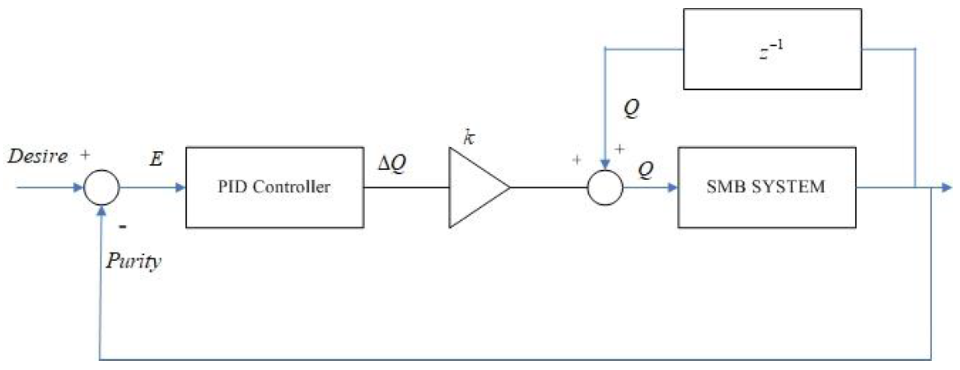
5. Controller Simulation

The successful implementation of a PID controller is contingent upon the precise tuning of its gains. Optimizing these PID gains is crucial for achieving optimal performance. In practical applications, it is necessary to discretize the continuous controller and sample it appropriately. The discrete form of the PID controller can be expressed as follows:

$$u(k)=K_{p}e(k)+K_d\Delta e(k)+K_i{\displaystyle \sum _{i=1}^{k}e(i)}$$

(80)

In the PID controller framework, the selected input variables comprise the error, the first-order error difference, and the integral error. The corresponding formula is articulated as follows:

$$e_1=desired B-C_{E,B}$$

(81)

$$e_2=desired A-C_{R,A}$$

(82)

$$e_3=e_1+e_2$$

(83)

$$\Delta e_1=e_1(k)-e_1(k-1)$$

(84)

$$\Delta e_2=e_2(k)-e_2(k-1)$$

(85)

$$\Delta e_3=\Delta e_1+\Delta e_2$$

(86)

$${\displaystyle \int e_1}={\displaystyle \sum _k{e}_1(k)}$$

(87)

$${\displaystyle \int e_2}={\displaystyle \sum _k{e}_2(k)}$$

(88)

$${\displaystyle \int e_3}={\displaystyle \int e_1}+{\displaystyle \int e_2}$$

(89)

To gain a deeper understanding of the evolving trends, a periodic averaging process is applied to the data. The formula used for a single-cycle moving average smoothing is as follows:

$${\stackrel{\_}{C}}_{E,B,t}={\displaystyle \frac{{\displaystyle {\int }_{t-T}^t{C}_{E,B,t}dt}}{T}}$$

(90)

$${\stackrel{\_}{C}}_{R,A,t}={\displaystyle \frac{{\displaystyle {\int }_{t-T}^t{C}_{R,A,t}dt}}{T}}$$

(91)

${\stackrel{-}{C}}_{E,B,t}$ is the B material purity of the extract port of average periodic, ${\stackrel{-}{C}}_{R,A,t}$ is the A material purity of the raffinate port of average periodic, and the control structure is shown in the Figure 8 below.

The flow rate control parameters for zones I, II, and III are configured as specified in

Table 3. PID control parameter setting.

Region	Kp	Kd	Ki
I	0.8	0.02	0.02
II	0.000097	0.00005	0.00005
III	0.02	0.003	0.003

. The resulting performance metrics are illustrated in Figure 9, Figure 10, Figure 11 and Figure 12. These figures provide a comprehensive analysis of the PID controller’s efficacy across various control objectives, as evaluated through three distinct case studies.

In the first set of experiments, the switching time parameter was set to 180 s, with the target control purity for material A set at 96% and for material B set at 94%. The actual control purity achieved was 95.44% for material A and 94% for material B. The results of the control are shown in Figure 9.

In the second set of experiments, the switching time parameter was set to 180 s, with the target control purity for both material A and material B set at 90%. The actual control purities achieved were 89.7% for material A and 89.42% for material B. The control results are shown in Figure 10. It can be observed from Figure 10 that a slight oscillation occurred when controlling the purity of material B.

In the third set of experiments, the switching time parameter was set to 178 s, with the target control purity for material A set at 93% and for material B set at 95%. The actual control purities achieved were 92.88% for material A and 95% for material B. The control performance is displayed in Figure 11.

In the fourth set of experiments, the switching time parameter was set to 180 s, with the target control purity for material A set at 94% and for material B set at 96%. The actual control purities achieved were 93.98% for material A and 96% for material B. The control results are shown in Figure 12.

From Figure 9, Figure 10, Figure 11 and Figure 12, it is evident that applying the controller within the discretized simulation system yields exceptional results. This lays a robust foundation for the subsequent optimization of the controller design. With a stable discretized simulation system, it becomes feasible to compare the various advantages and disadvantages of different controllers. Additionally, real-time online control is now achievable. Future research could leverage the discretized simulation system as a surrogate for the real system, implementing model predictive control.

In summary, the stability of the discretized dynamical system provides a superior platform for control simulation and efficiency improvements. Building on this, the stable discretized dynamical system not only enhances the accuracy of control simulations but also facilitates more robust analysis and development of advanced control strategies. The ability to conduct simulations in a controlled, virtual environment allows for the rigorous testing and fine-tuning of control algorithms without the constraints and risks associated with real-world experiments. Consequently, the insights gained from these simulations can lead to more effective and reliable control solutions when implemented in actual systems. This approach underscores the importance of a well-designed discretized model in advancing both theoretical research and practical applications in control system engineering.

6. Conclusions

Unlike methods based on finite elements, this study employs the Crank–Nicolson method to discretize the SMB system and rigorously establishes the reliability and computational convergence rate of the proposed method from a theoretical perspective. Subsequent simulation experiments were conducted to validate these findings. Initially, the impact of various parameter changes on the discretization process was examined, revealing that the discretized dynamical system of the SMB also exhibits high stability and reliability, with the computational model closely aligning with the actual system. Furthermore, the implementation of a controller within this discretized dynamical system has proven to be entirely feasible. This result provides a solid foundation for future controller optimization and real-time online control applications. The theoretical and practical significance of this study lies in the fact that the stability and reliability of the discretized model highlight its potential for robust control applications and efficient system design. The successful integration of the controller within this framework not only confirms its practicality but also paves the way for advancements in control strategies and performance optimization.

Subsequent research can focus on two aspects. One aspect is the design and development of controllers, specifically real-time online controllers based on finite difference methods and comparing the advantages and disadvantages of various controllers. The other aspect is the optimization of control based on the economic performance of the SMB system, utilizing high-efficiency simulations based on finite difference methods to enhance the feasibility of optimization control.

References

1. Rajendran, A.; Paredes, G.; Mazzotti, M. Simulated moving bed chromatography for the separation of enantiomers. J. Chromatogr. A 2009, 1216, 709–738. [Google Scholar] [CrossRef]
2. Chin, C.Y.; Wang, N.L. Simulated moving bed equipment designs. Sep. Purif. Rev. 2007, 33, 77–155. [Google Scholar] [CrossRef]
3. Kim, J.I.; Wankat, P.C.; Sungyong, M.; Yoon, K. Analysis of “focusing” effect in four zone SMB (simulated moving bed) unit for separation of xylose and glucose from biomass hydrolysate. J. Biosci. Bioeng. 2009, 108, 65–76. [Google Scholar] [CrossRef]
4. Suvarov, P.; Kienle, A.; Nobre, C.; Weireld, G.D.; Wouwer, A.V. Cycle to cycle adaptive control of simulated moving bed chromatographic separation processes. J. Process Control 2014, 24, 357–367. [Google Scholar] [CrossRef]
5. Choi, J.H.; Kang, M.S.; Lee, C.G.; Wang, N.H.L.; Mun, S. Design of simulated moving bed for separation of fumaric acid with a little fronting phenomenon. J. Chromatogr. A 2017, 1491, 75–86. [Google Scholar] [CrossRef]
6. Supelano, R.C.; Barreto, A.G., Jr.; Neto, A.S.A.; Secch, A.R.I. One-step optimization strategy in the simulated moving bed process with asynchronous movement of ports: A VariCol case study. J. Chromatogr. A 2020, 1634, 1672–1718. [Google Scholar]
7. Reinaldo, C.S.; Gomes, B.A.; Resende, S.A. Optimal performance comparison of the simulated moving bed process variants based on the modulation of the length of zones and the feed concentration. J. Chromatogr. A 2021, 1651, 462280. [Google Scholar]
8. Sá Gomes, P.M.D. Advances in Simulated Moving Bed: New Operating Modes: New Design Methodologies and Product (FlexSMB-LSRE) Development. Ph.D. Thesis, University of Porto (FEUP), Porto, Portugal, 2009. [Google Scholar]
9. Dunnebier, G.; Weirich, I.; Klatt, K.U. Computationally efficient dynamic modelling and simulation of simulated moving bed chromatographic processes with linear isotherms. Chem. Eng. Sci. 1998, 53, 2537–2546. [Google Scholar] [CrossRef]
10. Neto, A.S.A.; Secchi, A.R.; Souza, M.B.; Barreto, A.G. Nonlinear model predictive control applied to the separation of praziquantel in simulated moving bed chromatography. J. Chromatogr. A 2016, 1470, 42–49. [Google Scholar] [CrossRef]
11. Muhammed, T.; Tokay, B.; Conradie, A. Raising the Research Octane Number using an optimized Simulated Moving Bed technology towards greater sustainability and economic return. Fuel 2023, 337, 126864. [Google Scholar] [CrossRef]
12. Yan, Z.; Wang, J.S.; Wang, S.Y.; Li, S.J.; Wang, D.; Sun, W.Z. Model Predictive Control Method of Simulated Moving Bed Chromatographic Separation Process Based on Subspace System Identification. Math. Probl. Eng. 2019, 2019, 2391891. [Google Scholar] [CrossRef]
13. Leao, C.P.; Rodrigues, A.E. Transient and steady-state models for simulated moving bed processes: Numerical solutions. Comput. Chem. Eng. 2004, 28, 1725–1741. [Google Scholar] [CrossRef]
14. Majeed, H.; Hillestad, M.; Knuutila, H.; Svendsen, H.F. Predicting aerosol size distribution development in absorption columns. Chem. Eng. Sci. 2018, 192, 25–33. [Google Scholar] [CrossRef]
15. Kim, Y.; Kim, T.; Park, C.; Lee, J.; Cho, H.; Kim, M.; Moon, I. Development of novel flow distribution apparatus for simulated moving bed to improve degree of mixing. Comput. Chem. Eng. 2022, 156, 107553. [Google Scholar] [CrossRef]
16. Lee, W.S.; Lee, C.H. Dynamic modeling and machine learning of commercial-scale simulated moving bed chromatography for application to multi-component normal paraffin separation NSTL. Sep. Purif. Technol. 2022, 288, 120597. [Google Scholar] [CrossRef]
17. Li, S.; Wei, D.; Wang, J.S.; Yan, Z.; Wang, S.Y. Predictive control method of simulated moving bed chromatographic separation process based on piecewise affine. Int. J. Appl. Math. 2020, 50, 1–12. [Google Scholar]
18. Hoon, O.T.; Woo, K.J.; Hwan, S.S.; Hosoo, K.; Kyungmoo, L.; Min, L.J. Automatic control of simulated moving bed process with deep Q-network. J. Chromatogr. A 2021, 1647, 462073. [Google Scholar]
19. Natarajan, S.; Lee, J.H. Repetitive model predictive control applied to a simulated moving bed chromatography system. Comput. Chem. Eng. 2000, 24, 1127–1133. [Google Scholar] [CrossRef]
20. Klatt, K.U.; Hanisch, F.; Dunnebier, G. Mode-based control of a simulated moving bed chromatographic process for the separation of frutose and glucose. J. Process Control 2002, 12, 203–219. [Google Scholar] [CrossRef]
21. Carlos, V.; Alain, V.W. Combination of multi-model predictive control and the wave theory for the control of simulated moving bed plants. J. Chem. Eng. Sci. 2017, 66, 632–641. [Google Scholar]
22. Marrocos, H.; Iwakiri, I.G.I.; Martins, M.A.F.; Rodrigues, A.E.; Loureiro, J.M.; Ribeiro, A.M.; Nogueira, I.B.R. A long short-term memory based Quasi-Virtual Analyzer for dynamic real-time soft sensing of a Simulated Moving Bed unit. Appl. Soft Comput. 2022, 116, 108318. [Google Scholar] [CrossRef]
23. Santos, L.U.; Delgado, J.A.; Agueda, V.I. Recovery of a Succinic, Formic, and Acetic Acid Mixture from a Model Fermentation Broth by Simulated Moving Bed Adsorption with Methanol as a Desorbent. Ind. Eng. Chem. Res. 2022, 61, 672–683. [Google Scholar] [CrossRef]
24. Suzuki, K.; Harada, H.; Sato, K.; Okada, K.; Tsuruta, M.; Yajima, T.; Kawajiri, Y. Utilization of operation data for parameter estimation of simulated moving bed chromatography. J. Adv. Manuf. Process. 2022, 4, 10103. [Google Scholar] [CrossRef]
25. Yang, Y.; Chen, X.; Zhang, N. Optimizing control of adsorption separation processes based on the improved moving asymptotes algorithm. Adsorpt. Sci. Technol. 2018, 36, 1716–1733. [Google Scholar] [CrossRef]
26. Nogueira, I.B.; Martins, M.A.; Rodrigues, A.E.; Loureiro, J.M.; Ribeiro, A.M. Novel Switch Stabilizing Model Predictive Control Strategy Applied in the Control of a Simulated Moving Bed for the Separation of Bi-Naphthol Enantiomers. Ind. Eng. Chem. Res. 2020, 59, 1979–1988. [Google Scholar] [CrossRef]
27. Xie, C.-F.; Hong, Z.; Rey-Chue, H. Discrete Dynamic System Modeling for Simulated Moving Bed Processes. Mathematics 2024, 12, 1520. [Google Scholar] [CrossRef]
28. Crank, J.; Nicolson, P. A Practical Method for Numerical Evaluation of Solutions of Partial Differential Equations for the Heat Conduction Type; Cambridge University Press: Cambridge, UK, 1947; Volume 43, pp. 50–67. [Google Scholar]
Figure 1. Simulated moving bed operation process.
Axioms 13 00586 g001
Figure 2. Space split line of ( v l 1 , v l + 1 ) .
Axioms 13 00586 g002
Figure 3. SMB separation process on extract and raffinate.
Axioms 13 00586 g003
Figure 4. Axial concentration distribution curve.
Axioms 13 00586 g004
Figure 5. The concentration of A and B versus different adsorption rates ( H A = 0.5 0.25 ).
Axioms 13 00586 g005
Figure 6. The concentration of A and B versus different feed port concentrations ( C f = 4 6 ).
Axioms 13 00586 g006
Figure 7. The concentration of A and B versus different switching time ( θ = 178 182 ).
Axioms 13 00586 g007
Figure 8. PID controller for SMB.
Axioms 13 00586 g008
Figure 9. Group 1 control results (desired B = 94%, desired A = 96%, switch time = 180 s).
Axioms 13 00586 g009
Figure 10. Group 2 control results (desired B = 90%, desired A = 90%, switch time = 180 s).
Axioms 13 00586 g010
Figure 11. Group 3 control results (desired B = 95%, desired A = 93%, switch time = 178 s).
Axioms 13 00586 g011
Figure 12. Group 4 control results (desired B = 96%, desired A = 94%, switch time = 180 s).
Axioms 13 00586 g012