Dynamics of a New Four-Thirds-Degree Sub-Quadratic Lorenz-like System

Abstract

Aiming to explore the subtle connection between the number of nonlinear terms in Lorenz-like systems and hidden attractors, this paper introduces a new simple sub-quadratic four-thirds-degree Lorenz-like system, where $\dot{x}=a(y-x)$, $\dot{y}=cx-\sqrt[3]{x}z$, $\dot{z}=-bz+\sqrt[3]{x}y$, and uncovers the following property of these systems: decreasing the powers of the nonlinear terms in a quadratic Lorenz-like system where $\dot{x}=a(y-x)$, $\dot{y}=cx-xz$, $\dot{z}=-bz+xy$, may narrow, or even eliminate the range of the parameter c for hidden attractors, but enlarge it for self-excited attractors. By combining numerical simulation, stability and bifurcation theory, most of the important dynamics of the Lorenz system family are revealed, including self-excited Lorenz-like attractors, Hopf bifurcation and generic pitchfork bifurcation at the origin, singularly degenerate heteroclinic cycles, degenerate pitchfork bifurcation at non-isolated equilibria, invariant algebraic surface, heteroclinic orbits and so on. The obtained results may verify the generalization of the second part of the celebrated Hilbert’s sixteenth problem to some degree, showing that the number and mutual disposition of attractors and repellers may depend on the degree of chaotic multidimensional dynamical systems.

1. Introduction

As the fourteenth mathematical problem of the twenty-first century collected by Smale [1], revealing the nature of the Lorenz attractor has continued to be a hot topic of ongoing research in nonlinear science since its introduction [2,3,4,5,6,7,8]. As part of this ongoing effort, when studying the chaos of three-dimensional quadratic autonomous differential systems using the contraction map and boundary problem, Shilnikov et al. introduced the following classification: chaos of the Shilnikov homoclinic orbit, or heteroclinic orbit, or homoclinic and heteroclinic orbits hybrid orbit type, etc. [7]. Combining numerical technique and theoretical analysis, Kokubu et al. gave some explanation of Lorenz-like attractors from the viewpoint of the collapse of singularly degenerate heteroclinic cycles [9,10]. Llibre and Zhang applied homogeneous-weight polynomials and the method of characteristic curves to solve the linear partial differential equations in order to study invariant algebraic surface of the Lorenz system, the collapse of which may generate strange attractors [11]. Liao et al. argued that the existence of a global attractive compact set and having at least one positive Lyapunov exponent are the two sufficient conditions of a continuous system exhibiting chaos, and verified their findings using the chaotic Lorenz family [12,13]. Based on the algebraic structure and topological characterization, Letellier et al. introduced the concepts of Lorenz-like systems and attractors [8]. Chen separated the vector fields of Lorenz chaotic family into the linear and nonlinear parts [14], while others divided them into the conservative, dissipative and the external force field part [15,16,17].

However, Kuznetsov et al. turned their attention to the relationship between the degree of the considered model and Lorenz-like attractors and generalized the second part of the celebrated Hilbert’s sixteenth problem: the degree may control the number and mutual disposition of attractors and repellers [18,19]. Zhang and Chen reasserted this conjecture and coined two coexisting two-scroll Lorenz attractors from a cubic Lorenz system [20]. Motivated by that, Wang et al. guessed that decreasing the powers of x of the second and third equations of the quadratic Lorenz-like system [21] may widen the range of the parameter c for hidden attractors, and verified this via two sub-quadratic Lorenz-like analogues with degrees of four-thirds and six-fifths [22,23].

Now, one can not help but wonder what happens when decreasing the powers of x of the cross products $xz$ and $xy$ of the Lorenz-like system [21], especially for the self-excited and hidden attractors. To the best of our knowledge, little attention seems to have been paid to this problem. Furthermore, this newly reported Lorenz-like system also satisfies the second criterion of Sprott [24], i.e., the main contribution of this study, validating the generalization of the second part of the Hilbert’s sixteenth problem to some degree: the decrease in the powers of nonlinear terms may narrow or even eliminate the scope of some certain parameters for hidden Lorenz-like attractors, but enlarge it for self-excited attractors. This compelled us to carry out the research detailed here.

2. New Four-Thirds-Degree Lorenz-like System and Its Main Dynamics

By replacing the nonlinear term $c\sqrt[3]{x}$ in the sub-quadratic Lorenz-like system [22] with the linear one $cx$, we formulate the analogue as follows:

$$\left\{\begin{array}{cc}\dot{x}\hfill & =a(y-x),\hfill \\ \dot{y}\hfill & =cx-\sqrt[3]{x}z,a\ne 0,(b,c)\in {\mathbb{R}}^2,\hfill \\ \dot{z}\hfill & =-bz+\sqrt[3]{x}y.\hfill \end{array}\right.$$

(1)

In order to distinguish system (1) from the systems in [21,22,23], we must first present its basic dynamics in the following propositions. We have done this indentation.

Proposition 1.

(i) 

If $b=0$ (resp. $b\ne 0$ and $bc\le 0$), then $E_z=\left\{(0,0,z)\right|z\in \mathbb{R}\}$ is the non-isolated equilibria (resp. a single equilibrium point) of system (1).

(ii) 

If $bc>0$, then $E_{\pm }=(\pm \sqrt[2]{{\left(bc\right)}^3},\pm \sqrt[2]{{\left(bc\right)}^3},b{c}^2)$ is a pair of nontrivial equilibrium points in system (1) beside $E_0$.

Remark 1.

As in the systems in [21,22,23], a generic (resp. degenerate) pitchfork bifurcation at $E_0$ (resp. $E_z$) occurs in system (1) when $b\ne 0$ (resp. $c\ne 0$) and c (resp. b) passes through the zero value and $bc>0$.

Proposition 2.

For $a\ne 0$ and $(b,c)\in {\mathbb{R}}^2$ (resp. $b=0$ and $z\ne 0$), Table 1 (resp. Table 2) lists the local dynamics of $E_0$ (resp. $E_z$).

Table 1. The dynamical behaviors of $E_0$.

b	a	c	Property of ${\mathit{E}}_0$
<0	<0	<0	A 1D $W_{loc}^s$ and a 2D $W_{loc}^u$
		>0	A 3D $W_{loc}^u$
	>0	<0	A 2D $W_{loc}^s$ and a 1D $W_{loc}^u$
		>0	A 1D $W_{loc}^s$ and a 2D $W_{loc}^u$
>0	<0	<0	A 2D $W_{loc}^s$ and a 1D $W_{loc}^u$
		>0	A 1D $W_{loc}^s$ and a 2D $W_{loc}^u$
	>0	<0	A 3D $W_{loc}^s$
		>0	A 2D $W_{loc}^s$ and a 1D $W_{loc}^u$

Table 2. The dynamical behaviors of $E_z$.

z	a	Property of ${\mathit{E}}_{\mathit{z}}$
>0	<0	A 1D $W_{loc}^s$, a 1D $W_{loc}^c$ and a 1D $W_{loc}^u$
	>0	A 2D $W_{loc}^s$ and a 1D $W_{loc}^c$
<0	<0	A 2D $W_{loc}^u$ and a 1D $W_{loc}^c$
	>0	A 1D $W_{loc}^s$, a 1D $W_{loc}^c$ and a 1D $W_{loc}^u$

Remark 2.

As for the system in [22], using a linear analysis, one can easily obtain the characteristic equations of $E_0$ and $E_z$: $(\lambda +b)({\lambda }^2+a\lambda -ac)=0$ and $\lambda ({\lambda }^2+a\lambda -a(c-{\displaystyle \frac{z}{3\sqrt[3]{x^2}}}))$, where $x\to 0$, and from which Proposition 2 follows.

In the next proposition, let us discuss the local dynamics of $E_{\pm }$.

Proposition 3.

Make $S=\left\{\right(a,b,c\left)\right|a\ne 0,bc>0\}$, $S_1=\{(a,b,c)\in S:a+b>0,ab+bc-{\displaystyle \frac{2ac}{3}}>0,{\displaystyle \frac{2abc}{3}}>0\}$, $S_2=S\setminus S_1$ and

$$\begin{array}{c}{S}_1^1=\{(a,b,c)\in S_1:ab(a+b)-c[{\displaystyle \frac{a(2a+b)}{3}}-b^2]<0\},\hfill \\ S_1^2=\{(a,b,c)\in S_1:c={\displaystyle \frac{3ab(a+b)}{(a-b)(2a+3b)}}\},\hfill \\ S_1^3=\{(a,b,c)\in S_1:ab(a+b)-c[{\displaystyle \frac{a(2a+b)}{3}}-b^2]>0\}.\hfill \end{array}$$

Then, $E_{\pm }$ is unstable (resp. asymptotically stable) when $(a,b,c)\in S_1^1$ (resp. $S_1^3$). However, when $(a,b,c)\in S_1^2$, system (1) undergoes Hopf bifurcation at $E_{\pm }$.

As stated in [21] (Proposition 2.4, p. 2567) (resp. Proposition 3), the non-trivial equilibria $E_{\pm }$ of the following quadratic Lorenz-like system is

$$\left\{\begin{array}{cc}\dot{x}\hfill & =a(y-x),\hfill \\ \dot{y}\hfill & =cx-xz,a\ne 0,(b,c)\in {\mathbb{R}}^2,\hfill \\ \dot{z}\hfill & =-bz+xy,\hfill \end{array}\right.$$

(2)

(resp. system (1)) is asymptotically stable when $0<c<{\displaystyle \frac{a(a+b)}{a-b}}$ (resp. $0<c<{\displaystyle \frac{3ab(a+b)}{(a-b)(2a+3b)}}$). Due to ${\displaystyle \frac{3ab(a+b)}{(a-b)(2a+3b)}}<{\displaystyle \frac{a(a+b)}{a-b}}$, system (1) may experience chaotic behaviors coexisting with the unstable origin and stable $E_{\pm }$ in a narrower range of the parameter c in contrast to the quadratic one (2).

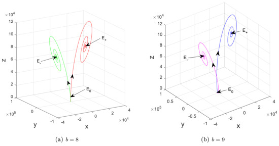
Likewise, for $(a,b)=(4,1)$, the $E_{\pm }$ of system (1) (resp. (2)) is asymptotically stable when $0<c<{\displaystyle \frac{20}{11}}$ (resp. $0<c<{\displaystyle \frac{20}{3}}$), and Figure 1 shows the periodic behavior rather than chaotic attractors displayed in system (2) [22] (Figure 3, p. 363).

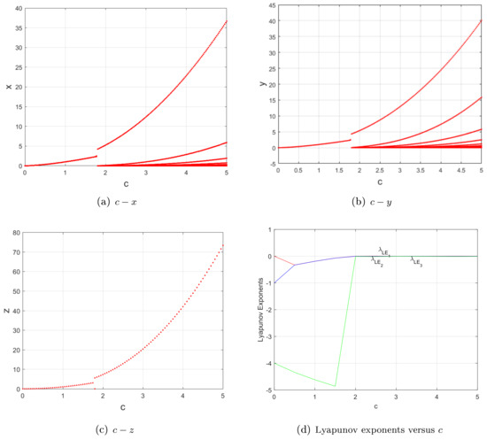
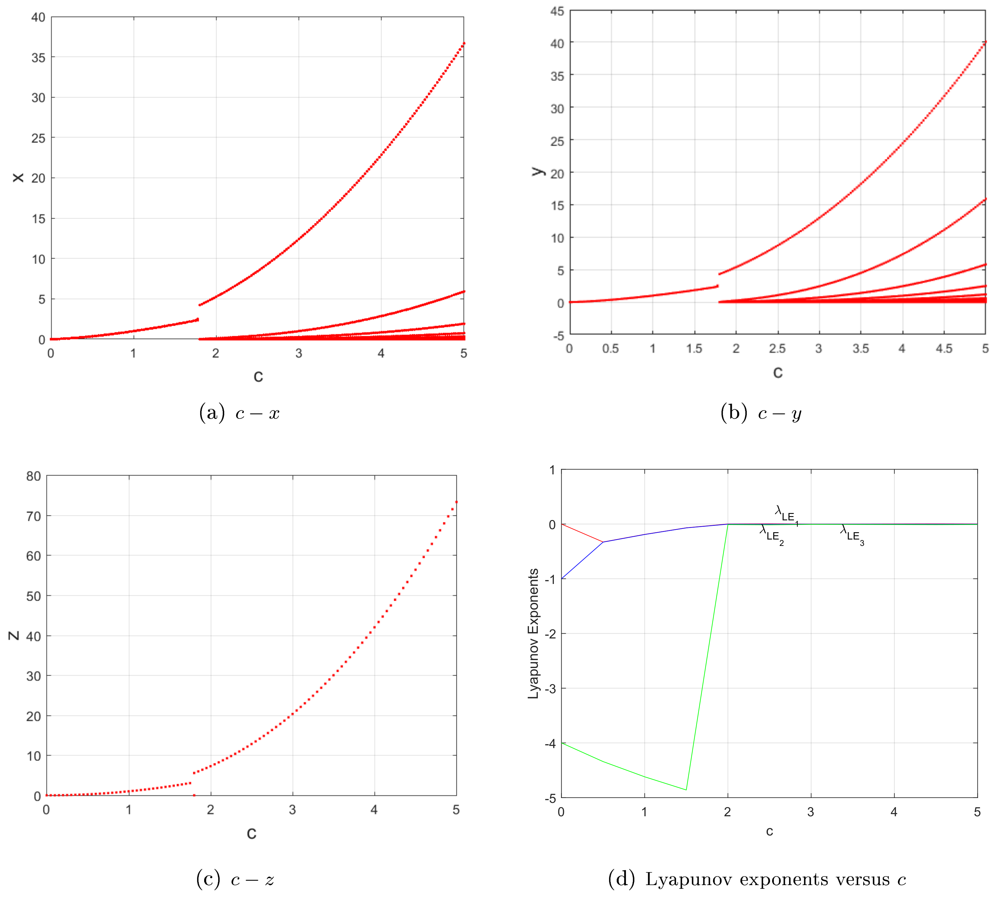
Figure 1. For $(a,b)=(4,1)$, $c\in [0,5]$ and $(x_0^1,y_0^1,z_0^1)=(0.13,1.3,1.6)\times {10}^{-7}$; (a–c) bifurcation diagrams; (d) Lyapunov exponents versus c of system (1). In contrast to system (2) [22] (Figure 3, p. 363), these figures suggest that the solutions for the system in (1) display stable equilibria and period orbits, rather than the self-excited and hidden attractors shown in the system in (2).

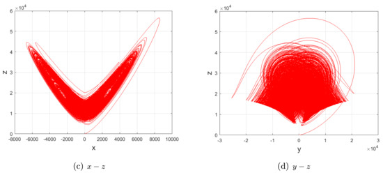
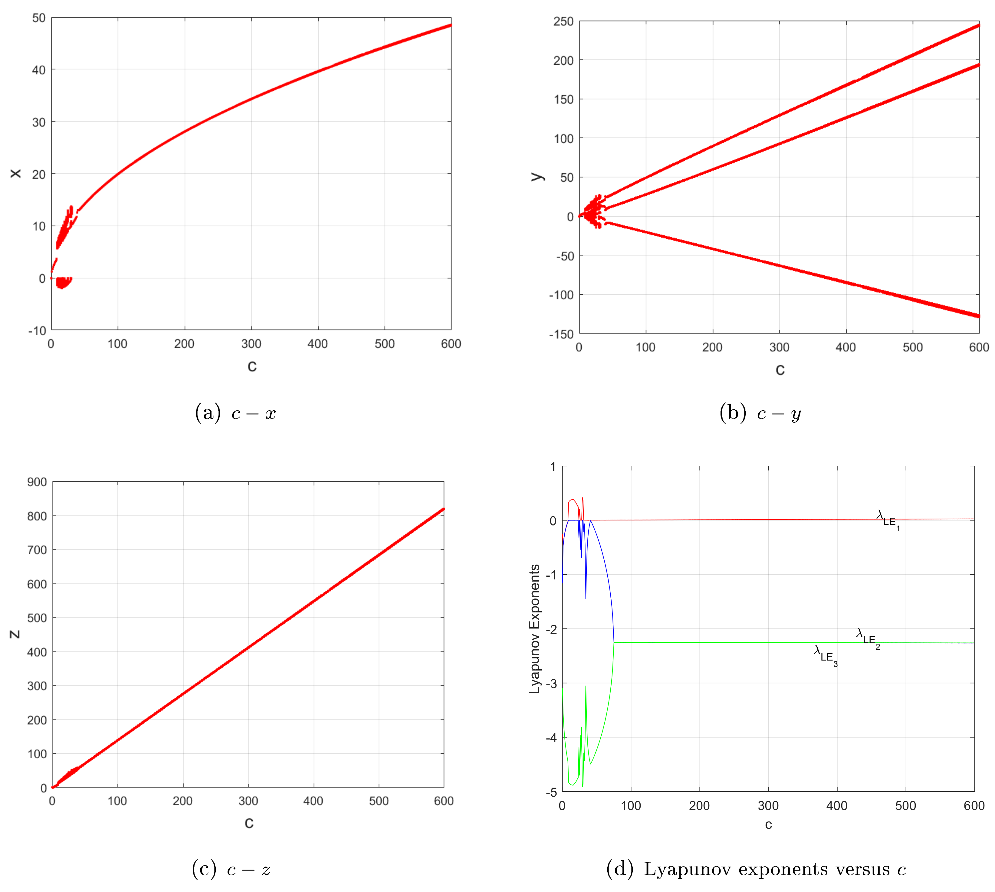
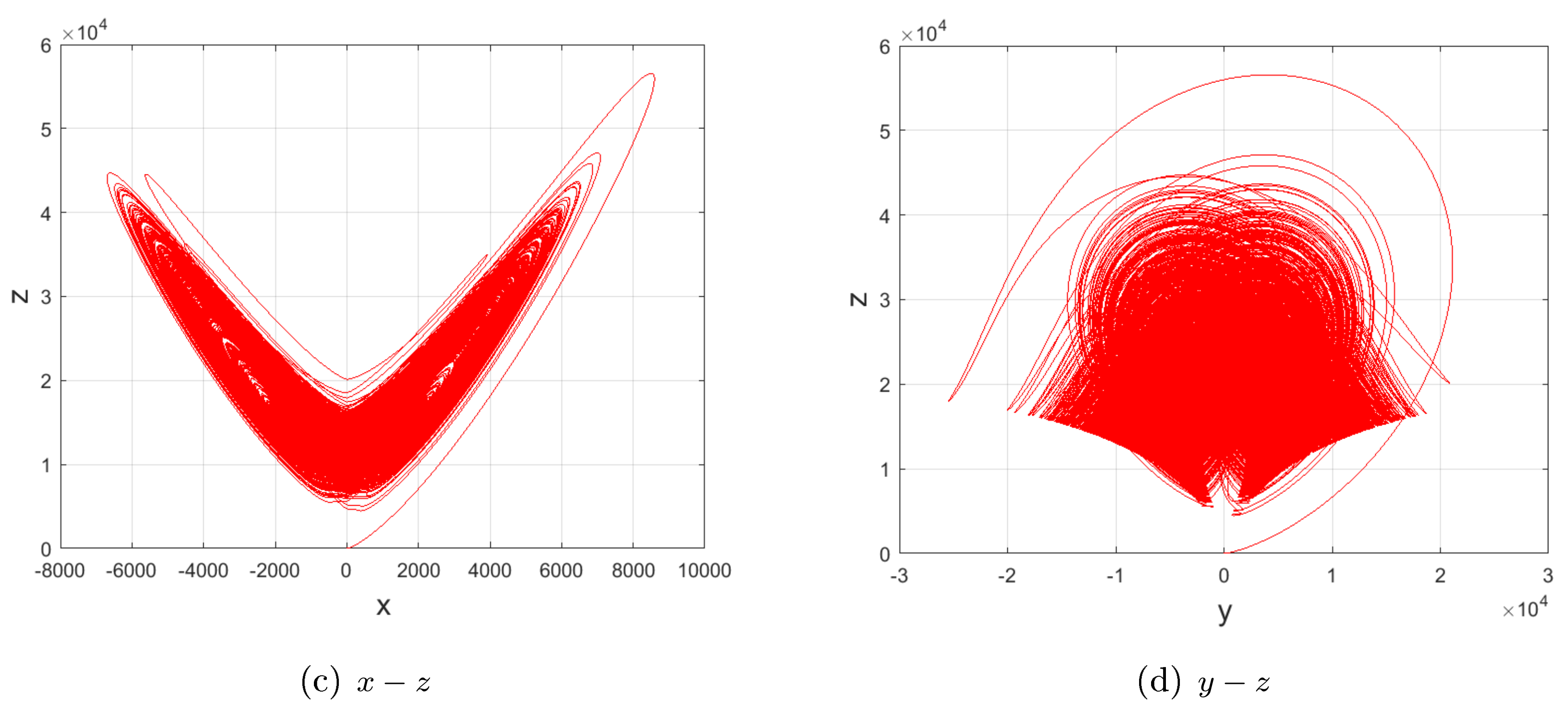
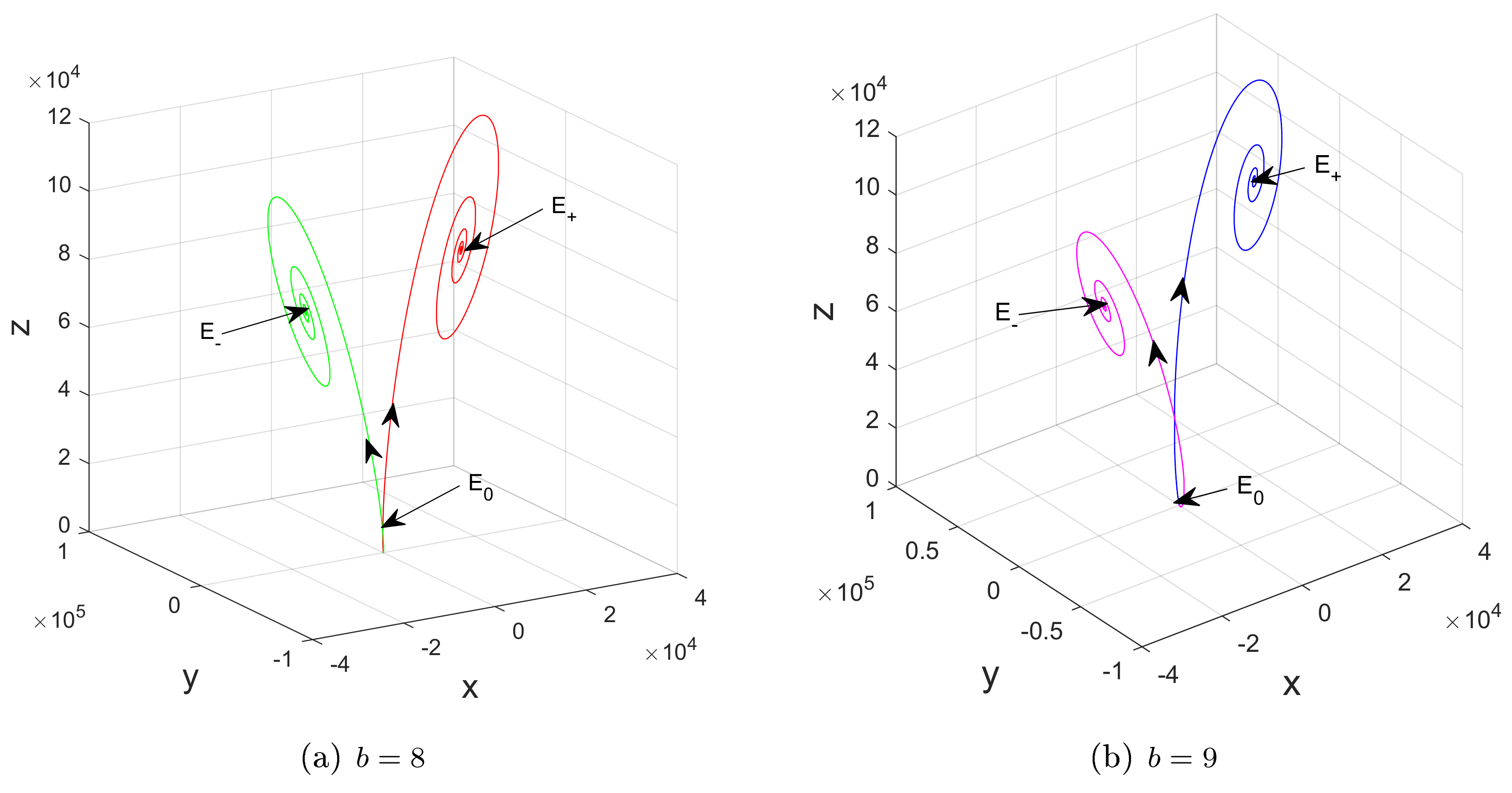
For $(a,b)=(3,1.5)$ and $c\in [0.1,599.1]$, the quadratic Lorenz-like system (2) mainly experiences periodic behaviors, whereas system (1) mainly experiences chaotic ones, as shown in Figure 2, Figure 3, Figure 4, Figure 5 and Figure 6.

Figure 2. For $(a,b)=(3,1.5)$, $c\in [0.1,599.1]$ and $(x_0^2,y_0^2,z_0^2)=(1.314,2.236,4.669)$; (a–c) bifurcation diagrams; (d) Lyapunov exponents versus c of system (2). The subfigures (a–c) are consistent with the subfigure (d), showing that system (2) mainly experiences periodic behaviors.

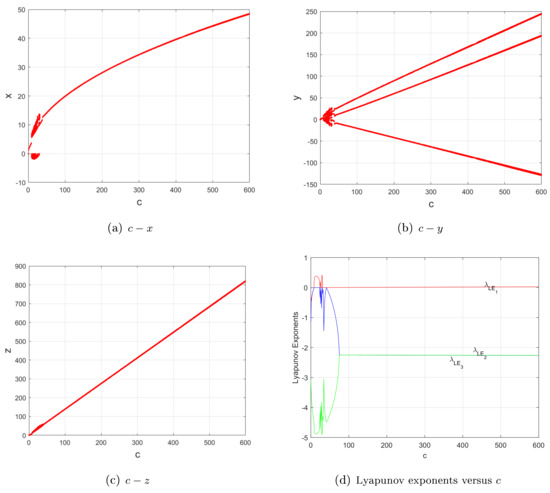
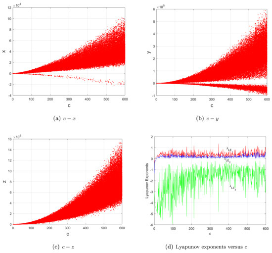
Figure 3. For $(a,b)=(3,1.5)$, $c\in [0.1,599.1]$ and $(x_0^2,y_0^2,z_0^2)=(1.314,2.236,4.669)$; (a–c) bifurcation diagrams; (d) Lyapunov exponents versus c of system (1). In contrast with Figure 2, the four subfigures show that system (1) mainly behaves in a similar way to self-excited attractors, verifying the introduced property, i.e., a decrease in powers of nonlinear terms of the quadratic Lorenz-like system (2) may narrow or even eliminate the range of the parameter c for hidden attractors, but enlarge it for self-excited attractors.

Figure 4. Phase portraits of system (1) for $(a,c,b)=(3,100,1.5)$ and $(x_0^2,y_0^2,z_0^2)=(1.314,2.236,4.669)$ illustrating the existence of two-scroll self-excited attractor suggested in Figure 3.

Figure 5. Poincaré cross-sections of system (1) for $(a,c,b)=(3,100,1.5)$ and $(x_0^2,y_0^2,z_0^2)=(1.314,2.236,4.669)$ showing the geometrical structure of the Lorenz-like attractor depicted in Figure 4.

Figure 6. Phase portraits of system (1) for $(a,c)=(1,36)$, (a) $b=0$, (b) $b=0.07$, and $(x_0^{1,3},y_0^{1,3},z_0^3)=(\pm 1.3\times {10}^{-8},\pm 1.3\times {10}^{-7},-1)$. Both figures imply that collapsing singularly degenerate heteroclinic cycles in system (1) create limited cycles rather than strange attractors.

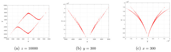
Therefore, compared with another two sub-quadratic Lorenz-like analogues [22] (Figures 1–2, p. 362), [23] (Property, Figures 2–4, p. 2450071-5-7) and Figure 2, Figure 3, Figure 4, Figure 5 and Figure 6, one may obtain the convincing argument:

Property. A decrease in the powers of nonlinear terms of the quadratic Lorenz-like system (2) may narrow or even eliminate the range of the parameter c for hidden attractors, but enlarge it for self-excited attractors.

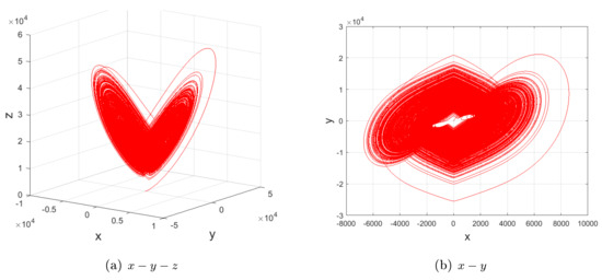
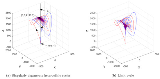
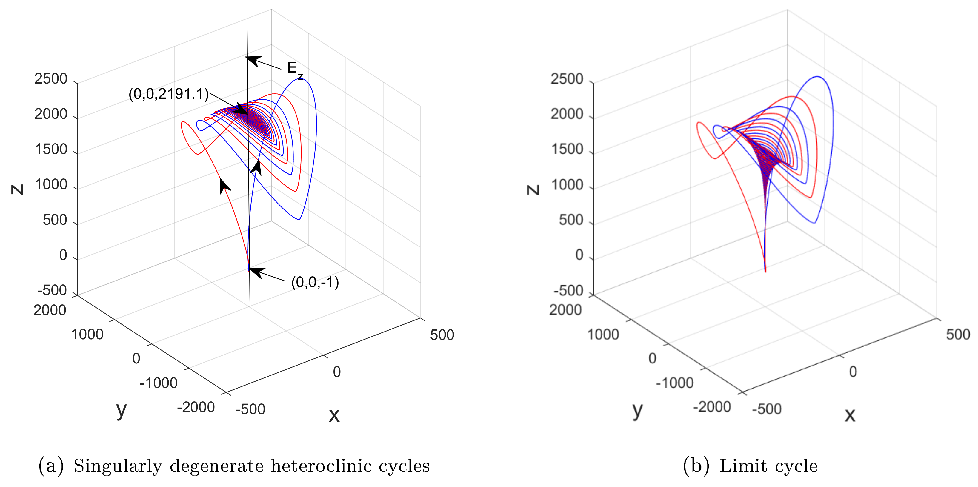
Meanwhile, unlike most of other Lorenz-like systems [9,10,22,23,25,26,27,28], the collapse of the singularly degenerate heteroclinic cycles in the system in (1) makes it hard to create strange attractors, as shown in the following numerical result.

$\mathbf{Numerical}\mathbf{Result}.\mathbf{2}.\mathbf{1}$ According to the dynamics of $E_z$ in Table 2, for $a>0$, $z_1<0$ and $t\to \infty$, the one-dimensional unstable manifold $W^u\left(E_z^1\right)$ ($E_z^1=(0,0,z_1)$) tending towards the stable $E_z^2=(0,0,z_2)$ with $z_2>0$ creates singularly degenerate heteroclinic cycles, as shown in Figure 3a. Moreover, a tiny perturbation in $b>0$ may change singularly degenerate heteroclinic cycles to limit cycles, as depicted in Figure 3b.

Remark 3.

When $(a,b)=(3,1.5)$, $E_{\pm }$ is asymptotically stable (resp. unstable) when $0<c<3.8571$ (resp. $c>3.8571$). However, when $(a,c,b)=(3,3.8571,1.5)$, the system in (1) undergoes Hopf bifurcation at $E_{\pm }$.

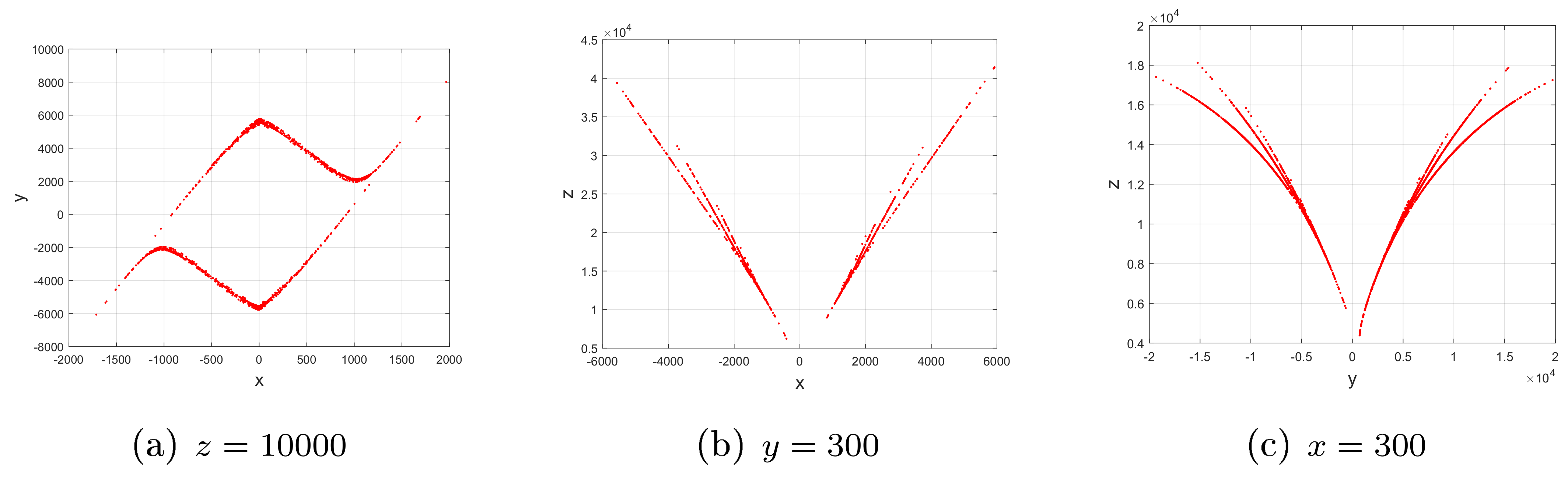
Finally, similarly to [21,22,23,26,28,29,30,31,32,33,34,35], we will discuss the heteroclinic orbits of the system in (1) and present it in the following proposition.

Proposition 4.

If $c>0$ and $3b\ge 4a>0$, then (a) the ω-limit of any one trajectory of system (1) is an equilibrium point; (b) system (1) has a pair of heteroclinic orbits to $E_0$ and $E_{\pm }$ but no homoclinic orbits.

Remark 4.

Generally speaking, the equilibria of heteroclinic orbits are all saddles or saddle-foci, or unstable nodes [7]. As heteroclinic orbits [21,22,23,26,28,29,30,31,32,33,34,35], those discussed in Proposition 4 are heteroclinic wiggles [7] (Figure 14.3.2, p. 439), which connect the stable $E_{\pm }$ and unstable $E_0$.

The rest of the paper is arranged as follows. Section 3 studies the stability and Hopf bifurcation of $E_{\pm }$ followed by the proof of Proposition 3. Section 4 discusses the heteroclinic orbits and the proof of Proposition 4 is outlined. A conclusion is drawn and the subject of future work is discussed in Section 5, particularly related to the the relationship between the degree and the Lorenz-like attractors.

3. Hopf Bifurcation

Using the theory of Hopf bifurcation, we then sketched a proof for Proposition 3.

Proof of Proposition 3.

First of all, the characteristic equation of $E_{\pm }$ is calculated:

$${\lambda }^3+(a+b){\lambda }^2+[ab+bc-{\displaystyle \frac{2ac}{3}}]\lambda +{\displaystyle \frac{2abc}{3}}=0.$$

(3)

Next, based on the Routh–Hurwitz criterion and Equation (3), we derived the stability of $E_{\pm }$; however, we have omitted its proof here.

$(a,b,c)\in S_1^2$, ${\lambda }_{1,2}=\pm \omega i=\pm \sqrt{ab[1+{\displaystyle \frac{(3b-2a)(a+b)}{(a-b)(2a+3b)}}]}i$ and ${\lambda }_3=-(a+b)$ are a pair of conjugate purely imaginary roots and one negative real root for Equation (3), respectively. Moreover, one has

$${\displaystyle \frac{d\mathit{Re}\left({\lambda }_1\right)}{dc}}{|}_{c=c^{*}}={\displaystyle \frac{ab-3b^2+2a^2}{6[{\omega }^2+{(a+b)}^2]}}={\displaystyle \frac{(3b+2a)(a-b)}{6[{\omega }^2+{(a+b)}^2]}}\ne 0,$$

from which the transversal condition is verified. Therefore, Hopf bifurcation happens at $E_{\pm }$. □

Next, we applied the project method [36,37] to compute the Lyapunov coefficients, aiming to determine the nondegeneracy (or stability) of the Hopf bifurcation at $E_{\pm }$.

Firstly, based on the time and coordinate transformation

$$(x,y,z,t)\to (x^3,y,z,{\displaystyle \frac{1}{3\sqrt[3]{x^2}}}t),$$

system (1) can be transformed to the equivalent one:

$$\left\{\begin{array}{cc}\dot{x}\hfill & =a(y-x^3),\hfill \\ \dot{y}\hfill & =3x^2(c{x}^3-xz),\hfill \\ \dot{z}\hfill & =3x^2(-bz+xy).\hfill \end{array}\right.$$

(4)

The $E_{\pm }$ of system (1) corresponds to $E^{1,2}=(\pm \sqrt{bc},\pm \sqrt{{\left(bc\right)}^3},b{c}^2)$ in system (4). One can verify the transversality of Hopf bifurcation at $E^{1,2}$.

In fact, the characteristic equation at $E^{1,2}$ is

$$\begin{array}{c}{\lambda }^3+3bc(a+b){\lambda }^2+3{\left(bc\right)}^2[(3b-2a)c+3ab]\lambda +18a{\left(bc\right)}^4=0,\hfill \end{array}$$

(5)

with ${\lambda }_{1,2}=\pm \omega i=\pm \sqrt{3{\left(b{c}_{*}\right)}^2[(3b-2a)c_{*}+3ab]}i$ and ${\lambda }_3=-3b{c}_{*}(a+b)<0$ when $(a,b,c)\in S_1^2$. We then obtained the following derivative

$${\displaystyle \frac{d\mathit{Re}\left({\lambda }_1\right)}{dc}}{|}_{c=c_{*}}={\displaystyle \frac{\mathsf{\Delta }}{2[{\omega }^2+9{\left(b{c}_{*}\right)}^2{(a+b)}^2]}}\ne 0,$$

where $\mathsf{\Delta }=-3b(a+b){\omega }^2+72a{b}^4{c}_{*}^3-3ab(a+b)[9b^2{c}_{*}^2(3b-2a)+18a{b}^3{c}_{*}]$, which thus verifies the transversality of Hopf bifurcation of $E^{1,2}$.

Then, the following transformation

$$(x,y,z)\to (x+\sqrt{b{c}_{*}},y+\sqrt{{\left(b{c}_{*}\right)}^3},z+b{\left(c_{*}\right)}^2),$$

converts system (4) into the resulting one

$$\begin{array}{cc}\left(\begin{array}{c}\dot{x}\\ \dot{y}\\ \dot{z}\end{array}\right)=\hfill & \left(\begin{array}{ccc}-3ab{c}_{*}& a& 0\\ 6b^2{c}_{*}^3& 0& -3\sqrt{{\left(b{c}_{*}\right)}^3}\\ 3{\left(b{c}_{*}\right)}^3& 3{\left(b{c}_{*}\right)}^2& -3b\sqrt{{\left(b{c}_{*}\right)}^3}\end{array}\right)\left(\begin{array}{c}x\\ y\\ z\end{array}\right)+3\left(\begin{array}{c}-a\sqrt{b{c}_{*}}{x}^2\\ 7c_{*}\sqrt{{\left(b{c}_{*}\right)}^3}{x}^2-3\sqrt{b{c}_{*}}xz\\ 3\sqrt{{\left(b{c}_{*}\right)}^5}{x}^2+4\sqrt{{\left(b{c}_{*}\right)}^3}xy-3b^2{c}_{*}xz\end{array}\right)\hfill \\ \hfill & +\left(\begin{array}{c}-a{x}^3\\ 9\sqrt{b{c}_{*}}(3c_{*}{x}^3-x^{2}z)\\ 9(-\sqrt{b{c}_{*}}b{x}^{2}z+{\left(b{c}_{*}\right)}^2{x}^3+2b{c}_{*}{x}^{2}y)\end{array}\right)+\left(\begin{array}{c}0\\ 3x^3(5c_{*}\sqrt{b{c}_{*}}x-z)\\ 3x^3(4\sqrt{b{c}_{*}}y-bz+\sqrt{{\left(b{c}_{*}\right)}^3}x)\end{array}\right)\hfill \\ \hfill & +\left(\begin{array}{c}0\\ 3c_{*}{x}^5\\ 3x^{4}y\end{array}\right).\hfill \end{array}$$

(6)

To compute the first Lyapunov coefficient $l_1$, one has to distill the following multi-linear symmetric functions from system (4)

$$B(x,y)=\left(\begin{array}{c}-6a\sqrt{b{c}_{*}}{x}_1{y}_1\\ 42c_{*}\sqrt{{\left(b{c}_{*}\right)}^3}{x}_1{y}_1-9\sqrt{b{c}_{*}}(x_1{y}_3+x_3{y}_1)\\ 18\sqrt{{\left(b{c}_{*}\right)}^5}{x}_1{y}_1+12\sqrt{{\left(b{c}_{*}\right)}^3}(x_1{y}_2+x_2{y}_1)-9b^2{c}_{*}(x_1{y}_3+x_3{y}_1)\end{array}\right),$$

$$C(x,y,z)=\left(\begin{array}{c}-6a{x}_1{y}_1{z}_1\\ 162\sqrt{b{c}_{*}}{c}_{*}{x}_1{y}_1{z}_1-18\sqrt{b{c}_{*}}(x_3{y}_1{z}_1+x_1{y}_3{z}_1+x_1{y}_1{z}_3)\\ -18b\sqrt{b{c}_{*}}(x_3{y}_1{z}_1+x_1{y}_3{z}_1+x_1{y}_1{z}_3)+54{\left(b{c}_{*}\right)}^2{x}_1{y}_1{z}_1+36b{c}_{*}(x_2{y}_1{z}_1+x_1{y}_2{z}_1+x_1{y}_1{z}_2)\end{array}\right)$$

When $l_1=0$, one needs to compute the other multi-linear symmetric functions to get the second Lyapunov exponent or the third or even higher order ones.

Due to complex algebraic structure of system (6) itself, it is difficult to obtain the explicit form of $l_1$. However, one can easily calculate it for a concrete problem, e.g., $(a,c,b)=(4,{\displaystyle \frac{20}{11}},1)$. Here, $E_{1,2}^{\prime }=(\pm \sqrt{{\displaystyle \frac{20}{11}}},\pm \sqrt{{({\displaystyle \frac{20}{11}})}^3},{\displaystyle \frac{400}{121}})$, whose eigenvalues are ${\lambda }_{1,2}=\pm \omega i=\pm 5.3713i$ and ${\lambda }_3=-27.2727$, and the transversality condition holds: ${\displaystyle \frac{d\mathit{Re}\left({\lambda }_1\right)}{dc}}{|}_{c=c_{*}={\displaystyle \frac{20}{11}}}\approx 0.5251>0$. Moreover, the $l_1$ of $E_{1,2}^{\prime }$ is discussed in the following proposition.

Proposition 5.

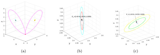
For $(a,c,b)=(4,{\displaystyle \frac{20}{11}},1)$, system (6) undergoes a Hopf bifurcation at $E_{1,2}^{\prime }$, for which the first Lyapunov coefficient is $l_1\approx -91.2608<0$, and thus $E_{1,2}^{\prime }$ are both weakly unstable foci. Because of ${\displaystyle \frac{d\mathit{Re}\left({\lambda }_1\right)}{dc}}\approx 0.5251>0$, the Hopf bifurcation at $E_{1,2}^{\prime }$ is supercritical. In a word, for $c>c_{*}={\displaystyle \frac{20}{11}}$ when it is close to $c_{*}={\displaystyle \frac{20}{11}}$, there is at least a pair of stable close orbits around the unstable $E_{1,2}^{\prime }$.

Proof. 

Based on the method proposed in [36,37], one can easily obtain the following expressions

$p=\left(\begin{array}{c}0.0318+0.0349i\\ 0.0173+0.0233i\\ -0.00019--0.02346i\end{array}\right),$ $q=\left(\begin{array}{c}4\\ 21.8181+5.3712i\\ 23.5357-15.9337i\end{array}\right),$ $h_{11}=\left(\begin{array}{c}-108.4504\\ -462.1017\\ -435.16077\end{array}\right),$

$h_{20}=\left(\begin{array}{c}55.35369+20.7412i\\ 375.6721+261.7939i\\ 750.3901-236.67872i\end{array}\right),$ $G_{21}=-182.5216-1713.4399i$ and $l_1={\displaystyle \frac{1}{2}}{G}_{21}=-91.2608$. Since ${\displaystyle \frac{d\mathit{Re}\left({\lambda }_1\right)}{dc}}\approx 0.5251>0$, the Hopf bifurcation at $E_{1,2}^{\prime }$ is supercritical. Namely, when $c=1.8182>c_{*}$, there exists a pair of stable close orbits around the unstable $E_{1,2}^{″}=(\pm 1.3484,\pm 2.4517,3.3059)$ for system (4), i.e., $E_{\pm }=(\pm 2.4517,\pm 2.4517,3.3059)$ of system (1), as illustrated in Figure 7. This finishes the proof. □

Figure 7. Phase portraits of system (1) for $(a,c,b)=(4,1.8182,1)$ and (a) $(x_0^{1,3},y_0^{1,3},z_0^4)=(\pm 0.13,\pm 1.3,1.6)\times {10}^{-7}$, $(x_0^{3,4},y_0^{3,4},z_0^4)=(\pm 2.4,\pm 2.41,3.3)$ and $(x_0^{5,6},y_0^{5,6},z_0^5)=(\pm 2.39,\pm 2.4,3.32)$, (b) $(x_0^3,y_0^3,z_0^4)=(2.4,2.41,3.3)$, $(x_0^5,y_0^5,z_0^5)=(2.39,2.4,3.32)$, (c) $(x_0^4,y_0^4,z_0^4)=(-2.4,-2.41,3.3)$ and $(x_0^6,y_0^6,z_0^5)=(-2.39,-2.4,3.32)$, showing at least five limit cycles for system (1) when Hopf bifurcation occurs at $E_{\pm }$ i.e., two around $E_{+}$, two around $E_{-}$ and one around $E_{\pm }$.

In the next section, we will study the existence of heteroclinic orbits in system (1). For the sake of our argument, we list the following symbols:

(1) $\psi (t;{\psi }_0)=(x(t;x_0),y(t;y_0),z(t;z_0))$: a solution for system (1) with the initial condition ${\psi }_0=(x_0,y_0,z_0)$.

(2) ${\gamma }^{-}=\left\{{\psi }_{-}(t;{\psi }_0)\right|{\psi }_{-}(t;{\psi }_0)=(-x_{+}(t;x_0),-y_{+}(t;y_0),z_{+}(t;z_0))\in W_{-}^u\left(E_0\right),t\in \mathbb{R}\}$ (resp. ${\gamma }^{+}=\left\{{\psi }_{+}(t;{\psi }_0)\right|{\psi }_{+}(t;{\psi }_0)=(x_{+}(t;x_0),y_{+}(t;y_0),z_{+}(t;z_0))\in W_{+}^u\left(E_0\right),t\in \mathbb{R}\}$): the negative (resp. positive) branch of $W^u\left(E_0\right)$ with $-x_{+}<0$ (resp. $x_{+}>0$) when $t\to -\infty$.

4. Existence of Heteroclinic Orbit

In this section, as in [21,22,23,26,28,29,30,31,32,33,34,35], with a suitable choice of Lyapunov functions, the proof of Proposition 4 can be divided into two stages: (1) $3b-4a>0$, (2) $3b-4a=0$.

4.1. $3b-4a>0$

This subsection introduces the first Lyapunov function

$$V_1(\psi (t;{\psi }_0))={\displaystyle \frac{1}{2}}[b(b-{\displaystyle \frac{4a}{3}}){(y-x)}^2+{(-bz+\sqrt[3]{x^4})}^2+{\displaystyle \frac{3b-4a}{6a}}{(-bc\sqrt[3]{x^2}+\sqrt[3]{x^4})}^2+{\displaystyle \frac{3b-4a}{12a}}{(-b^2{c}^2+\sqrt[3]{x^4})}^2]$$

and the following assertions:

Lemma 1.

If $c>0$ and $3b-4a>0$, then we have the following results:

1. 

Assume $\exists t_{1,2}$, $t_1<t_2$ and $V_1\left(\psi (t_1;{\psi }_0)\right)=V_1\left(\psi (t_2;{\psi }_0)\right)$. ${\psi }_0$ is one of the stationary points.

2. 

If ${lim}_{t\to -\infty }\psi (t;{\psi }_0)=E_0$ and $x(t_3;x_0)<0$, $\exists t_3\in \mathbb{R}$, then we arrive at $V_1\left(E_0\right)>V_1\left(\psi (t;{\psi }_0)\right)$ and $x(t;x_0)<0$, $\forall t\in \mathbb{R}$. Namely, ${\psi }_0\in {\gamma }^{-}$.

Proof. 

(1) By taking the derivative of $V_1$ with respect to $\psi (t;{\psi }_0)$, we arrive at

$$\begin{array}{ccc}{\displaystyle \frac{d{V}_1\left(\psi (t;{\psi }_0)\right)}{dt}}{|}_{\left(1\right)}\hfill & =\hfill & -ab(b-{\displaystyle \frac{4a}{3}}){(y-x)}^2-b{(-bz+\sqrt[3]{x^4})}^2,\hfill \end{array}$$

(7)

and derive

$$y(t;y_0)\equiv x(t;x_0),bz(t;z_0)\equiv \sqrt[3]{x^4}(t;x_0),$$

(8)

under the condition of (1), $\forall t\in (t_1,t_2)$.

Based on system (1) and Equation (8), the identities $\dot{x}(t;x_0)\equiv \dot{y}(t;y_0)\equiv \dot{z}(t;z_0)\equiv 0$ hold, $\forall t\in (t_1,t_2)$. Namely, ${\psi }_0$ is a fixed point.

(2) Now, $\forall t\in \mathbb{R}$, we prove the fact $V_1\left(E_0\right)>V_1\left(\psi (t;{\psi }_0)\right)$. If not, $\exists t\in \mathbb{R}$, $V_1\left(E_0\right)\le V_1\left(\psi (t;{\psi }_0)\right)$. In fact, the first assertion suggests that ${\psi }_0$ is just an equilibrium point, contradicting the assumption that ${lim}_{t\to -\infty }\psi (t;{\psi }_0)=E_0$ and $x(t_3;x_0)<0$. In a word, $V_1\left(E_0\right)>V_1\left(\psi (t;{\psi }_0)\right)$, $\forall t\in \mathbb{R}$.

Next, let us prove $x(t;x_0)<0$, $\forall t\in \mathbb{R}$. Otherwise, $x(t_4;x_0)\ge 0$, $\exists t_4\in \mathbb{R}$. Since $x(t_3;x_0)<0$, $t_3\in \mathbb{R}$, one arrives at $x(t_5;x_0)=0$, $\exists t_5\in \mathbb{R}$. Due to $V_1\left(E_0\right)>V_1\left(\psi (t;{\psi }_0)\right)$, $\forall t\in \mathbb{R}$, one gets $\psi (t_5;{\psi }_0)\in \left\{(x,y,z)|V_1(x,y,z)<V_1\left(E_0\right)\right\}\cap \left\{(x,y,z)|x=0\right\}.$ Further, the following statement is derived, $\left\{(x,y,z)\right|V_1(x,y,z)<V_1\left(E_0\right)\}\cap \left\{(x,y,z)\right|x=0\}=\{(0,y,z)|{\displaystyle \frac{1}{2}}[b(b-{\displaystyle \frac{4a}{3}})y^2+b^2{z}^2+{\displaystyle \frac{(3b-4a)b^4{c}^4}{12a}}]<{\displaystyle \frac{(3b-4a)b^4{c}^4}{24a}}\}=\varnothing ,$ which is impossible. As a result, one arrives at $x(t;x_0)<0$, for all $t\in \mathbb{R}$. This ends the proof. □

Lemma 2.

When $c>0$ and $3b>4a>0$, all of the solutions for system (1) tend towards an equilibrium point such as $t\to \infty$. Namely, system (1) has no closed orbits.

Proof. 

On the basis of Equation (7), one derives ${lim}_{t\to +\infty }{V}_1\left(\psi (t;{\psi }_0)\right)=\mathsf{\Phi }\left({\psi }_0\right)$, $0\le V_1\left(\psi (t;{\psi }_0)\right)\le V_1\left(\psi (0;{\psi }_0)\right)=V_1\left({\psi }_0\right),\forall t\ge 0,$ and obtains that $x(t;x_0)$, $y(t;y_0)$ and $z(t;z_0)$ are all bounded, $t\in [0,+\infty )$, i.e., $\psi (t;{\psi }_0)$ is bounded.

Denoting the $\omega$-limit set of $\psi (t;{\psi }_0)$ by $\mathsf{\Omega }\left({\psi }_0\right)\ne \varnothing$. For $\forall w\in \mathsf{\Omega }\left({\psi }_0\right)$, $\exists \left\{t_n\right\}$, we have

$$\underset{n\to +\infty }{lim}{t}_n=+\infty ,\underset{n\to +\infty }{lim}\psi (t_n,{\psi }_0)=w.$$

Next, for all $t\in \mathbb{R}$, $\psi (t;w)=\underset{n\to +\infty }{lim}\psi (t;\psi (t_n;{\psi }_0))=\underset{n\to +\infty }{lim}\psi (t+t_n;{\psi }_0)$ suggests $V_1\left(\psi (t;w)\right)$ = $V_1[\underset{n\to +\infty }{lim}\psi (t;\psi (t_n;$${\psi }_0\left)\right)]=\underset{n\to +\infty }{lim}{V}_1\left(\psi (t+t_n;{\psi }_0)\right)=\mathsf{\Phi }\left({\psi }_0\right).$ As a result, $w\in \{E_{+},E_{-},E_0\}$. Because of connectedness of $\mathsf{\Omega }\left({\psi }_0\right)$, one only deduces $\mathsf{\Omega }\left({\psi }_0\right)=\left\{E_{+}\right\}$, $\mathsf{\Omega }\left({\psi }_0\right)=\left\{E_{-}\right\}$ or $\mathsf{\Omega }\left({\psi }_0\right)=\left\{E_0\right\}$, yielding that $\psi (t;{\psi }_0)$ approaches an equilibrium point such as $t\to +\infty$. The proof is completed. □

Lastly, one considers the existence of heteroclinic orbits with the help of above two lemmas.

Theorem 1.

When $c>0$ and $3b>4a>0$, the following two statements hold.

1. 

System (1) has no homoclinic orbits.

2. 

A pair of heteroclinic orbits at $E_{\pm }$ and $E_0$ exists in system (1).

Proof. 

For $c>0$ and $3b>4a>0$, one firstly shows that homoclinic orbits at $E_{\pm }$ or $E_0$ do not exist in system (1). If not, a homoclinic orbit at $E_0$, $E_{+}$ or $E_{-}$ can be denoted by $\psi \left(t\right)$, i.e., $\underset{t\to \pm \infty }{lim}\psi \left(t\right)=e^{\pm }$, where $e^{-}=e^{+}\in \{E_{-},E_{+},E_0\}$.

From Equation (7), one obtains

$$V_1\left(e^{-}\right)\ge V_1\left(\psi \left(t\right)\right)\ge V_1\left(e^{+}\right).$$

(9)

In both cases, we obtain the fact that $V_1\left(e^{-}\right)=V_1\left(e^{+}\right)$ and further arrive at $V_1\left(\psi \left(t\right)\right)\equiv V_1\left(e^{+}\right)$. From the first statement in Lemma 1, $\psi \left(t\right)$ is only an equilibrium point. Namely, homoclinic orbits at $E_0$, $E_{+}$ or $E_{-}$ are non-existent.

Then, let us prove that ${\gamma }^{-}$ is a heteroclinic orbit at $E_0$ and $E_{-}$, i.e., $\underset{t\to +\infty }{lim}p\left(t\right)=E_{-}$. From the concept of ${\gamma }^{-}$ and Lemma 1, we only arrive at $-x_{+}\left(t\right)<0$, for all $t\in \mathbb{R}$, yielding $\underset{t\to +\infty }{lim}{\psi }_{-}\left(t\right)\ne E_0$. As a result, $\underset{t\to +\infty }{lim}{\psi }_{-}\left(t\right)=E_{-}$ is true.

Finally, let us prove the uniqueness of ${\gamma }^{-}$.

Let ${\psi }_1\left(t\right)=(x_1\left(t\right),y_1\left(t\right),z_1\left(t\right))$ be a solution for system (1) such that $\underset{t\to \pm \infty }{lim}{\psi }_1\left(t\right)=e_1^{\pm }$, and $\{e_1^{-},e_1^{+}\}=\{E_0,E_{-}\}.$ Like Equation (9), one gets $V_1\left(e_1^{-}\right)\ge V_1\left({\psi }_1\left(t\right)\right)\ge V_1\left(e_1^{+}\right)$, $\forall t\in \mathbb{R}$, from Equation (8). Due to $V_1\left(E_0\right)>V_1\left(E_{-}\right)$, one derives $e_1^{-}=E_0$ and $e_1^{+}=E_{-}$, i.e.,

$$\underset{t\to -\infty }{lim}{\psi }_1\left(t\right)=E_0,\underset{t\to +\infty }{lim}{\psi }_1\left(t\right)=E_{-},$$

which leads to ${\psi }_1\left(t\right)\in {\gamma }^{-}$ from the second assertion of Lemma 1. Since system (1) is axis-symmetrical with respect to the z-axis, a single heteroclinic orbit ${\gamma }^{+}$, i.e., the ones at $E_0$ and $E_{+}$, also exists in system (1). This completes the proof. □

4.2. $3b-4a=0$

Firstly, we introduce another Lyapunov function

$$V_2\left(\psi (t;{\psi }_0)\right)={\displaystyle \frac{1}{2}}[{(y-x)}^2+{\displaystyle \frac{3}{8a^2}}{(-{\displaystyle \frac{4ac}{3}}\sqrt[3]{x^2}+\sqrt[3]{x^4})}^2+{\displaystyle \frac{3}{16a^3}}{(-{\displaystyle \frac{16a^2{c}^2}{9}}+\sqrt[3]{x^4})}^2]$$

from which the following lemma is deduced:

Lemma 3.

When $c>0$ and $3b=4a>0$, one arrives at the following four assertions.

(i) If ${lim}_{t\to -\infty }\psi (t;{\psi }_0)$ is bounded, then $Q\left(\psi (t;{\psi }_0)\right)=z(t;z_0)-{\displaystyle \frac{3}{4a}}\sqrt[3]{x^4}(t;x_0)=0$.

(ii) If $4az(t;z_0)=3\sqrt[3]{x^4}(t;x_0)$, then ${\displaystyle \frac{d{V}_2\left(\psi (t;{\psi }_0)\right)}{dt}}{|}_{\left(1\right)}=-a{(y-x)}^2\le 0.$

(iii) If $4az(t;z_0)=3\sqrt[3]{x^4}(t;x_0)$ and $V_2\left(\psi (t_1;{\psi }_0)\right)=V_2\left(\psi (t_2;{\psi }_0)\right)$, $\exists t_{1,2}$, $t_1<t_2$, then ${\psi }_0$ is an equilibrium point.

(iv) If ${lim}_{t\to -\infty }\psi (t;{\psi }_0)=E_0$ and $x(t_3;x_0)<0$, $\exists t_3\in \mathbb{R}$, then $V_2\left(E_0\right)>V_2\left(\psi (t;{\psi }_0)\right)$ and $x(t;x_0)<0$, $\forall t\in \mathbb{R}$. Namely, ${\psi }_0\in {\gamma }^{-}$.

Proof. 

(i) When $c>0$ and $3b=4a>0$, the derivative of $Q\left(\psi (t;{\psi }_0)\right)=z(t;z_0)-{\displaystyle \frac{3}{4a}}\sqrt[3]{x^4}(t;x_0)$ is calculated as follows: ${\displaystyle \frac{dQ\left(\psi (t;{\psi }_0)\right)}{dt}}{|}_{\left(1\right)}=-{\displaystyle \frac{4a}{3}}Q\left(\psi (t;{\psi }_0)\right)$, i.e.,

$$Q\left(\psi (t;{\psi }_0)\right)=Q\left(\psi (\tau ;{\psi }_0)\right)e^{-{\displaystyle \frac{4a}{3}}(t-\tau )},\forall \tau ,t\in \mathbb{R}.$$

(10)

Since ${lim}_{\tau \to -\infty }\psi (\tau ;{\psi }_0)$ is bounded, Equation (10) yields $Q\left(\psi (t;{\psi }_0)\right)\equiv 0$, i.e., $z(t;z_0)\equiv {\displaystyle \frac{3}{4a}}\sqrt[3]{x^4}(t;x_0)$.

(ii) The fact that $4az(t;z_0)\equiv 3\sqrt[3]{x^4}(t;x_0)$ and system (1) result in Conclusion (ii) of Lemma 3.

(iii) Based on assumed conditions and the above statement, we obtain ${\displaystyle \frac{d{V}_2\left(\psi (t,{\psi }_0)\right)}{dt}}{|}_{\left(1\right)}=0$, for all $t\in (t_1,t_2)$, i.e.

$$y(t;y_0)\equiv x(t;x_0).$$

(11)

In virtue of $\dot{x}$, Equation (11) and $4az(t;z_0)\equiv 3\sqrt[3]{x^4}(t;x_0)$, one deduces

$$\dot{x}(t;x_0)\equiv \dot{y}(t;y_0)\equiv \dot{z}(t;z_0)\equiv 0,\forall t\in (t_1,t_2).$$

Hence, ${\psi }_0$ is only an equilibrium point.

(iv) First of all, one shows that $V_2\left(E_0\right)>V_2\left(\psi (t;{\psi }_0)\right)$, $\forall t\in \mathbb{R}$. If not, $V_2\left(E_0\right)\le V_2\left(\psi (t_0;{\psi }_0)\right)$, $\exists t_0\in \mathbb{R}$. In addition, the first, second and third assertions yield that ${\psi }_0$ is an equilibrium point, which contradicts ${lim}_{t\to -\infty }\psi (t;{\psi }_0)=0$ and $x(t_3;x_0)<0$. Namely, we find that $V_2\left(E_0\right)>V_2\left(\psi (t;{\psi }_0)\right)$ holds for $\forall t\in \mathbb{R}$.

Then, we prove $x(t;x_0)<0$, $\forall t\in \mathbb{R}$. If not, $\exists t_4\in \mathbb{R}$, such that $x(t_4;x_0)\ge 0$. Due to $x(t_3;x_0)<0$, $\exists t_5\in \mathbb{R}$, such that $x(t_5;x_0)=0$. Since $V_2\left(E_0\right)>V_2\left(\psi (t;{\psi }_0)\right)$, $\forall t\in \mathbb{R}$, we obtain $\psi (t_5;{\psi }_0)\in \left\{(x,y,z)\right|V_2(x,y,z)<V_2\left(E_0\right)\}\cap \left\{(x,y,z)\right|x=0\}.$ On the other hand, $\{(x,y,z)|V_2(x,y,z)<V_2\left(E_0\right)\}\cap \left\{(x,y,z)\right|x=0\}=\{(0,y,z)|{\displaystyle \frac{1}{2}}[y^2+{\displaystyle \frac{16a{c}^4}{27}}]<{\displaystyle \frac{8a{c}^4}{27}}\}$$=\varnothing$. As such, a contradiction happens. Therefore, $x(t;x_0)<0$ holds, $\forall t\in \mathbb{R}$. □

Lemma 4.

Set $c>0$ and $3b=4a>0$. If $\psi (t,{\psi }_0)$ is bounded when $t\to -\infty$, then ${lim}_{t\to -\infty }\psi (t,{\psi }_0)\to E_0$, or $E_{\pm }$. In a word, there are no closed orbits in system (1).

Proof. 

From the first and second assertion of Lemma 3, ${lim}_{t\to -\infty }{V}_2\left(\psi (t;{\psi }_0)\right)=\mathsf{\Psi }\left({\psi }_0\right)$ exists. Assume $h\in \alpha \left({\psi }_0\right)$, i.e., $\exists \left\{t_n\right\}$, we have ${lim}_{t_n\to -\infty }\psi (t_n;{\psi }_0)=h,n\to +\infty .$ For all $t\in \mathbb{R}$,

$$\psi (t;h)=\underset{n\to +\infty }{lim}\psi (t;\psi (t_n;{\psi }_0))=\underset{n\to +\infty }{lim}\psi (t+t_n;{\psi }_0)$$

leads to

$$\left\{\begin{array}{c}\psi (t;h)\mathrm{is}\mathrm{bounded},\forall t\in \mathbb{R},\hfill \\ V_2\left(\psi (t;h)\right)=\underset{n\to +\infty }{lim}{V}_2\left(\psi (t+t_n;{\psi }_0)\right)=\mathsf{\Psi }\left({\psi }_0\right).\hfill \end{array}\right.$$

(12)

On the basis of Lemma 3, one obtains $h\in \{E_{-},E_0,E_{+}\}$. Therefore,

$$\alpha \left({\psi }_0\right)\subseteq \{E_{-},E_0,E_{+}\}.$$

Because $\alpha \left({\psi }_0\right)$ is connected, one derives $\alpha \left(q_0\right)=\left\{E_{-}\right\}$, or $\alpha \left(q_0\right)=\left\{E_0\right\}$, or $\alpha \left(q_0\right)=\left\{E_{+}\right\}$, suggesting that ${lim}_{n\to +\infty }\psi (t;{\psi }_0)$ approaches an equilibrium point. The proof is completed. □

Theorem 2.

When $3b=4a>0$ and $c>0$, we derive the statements as follows.

(i) There are no homoclinic orbits in system (1).

(ii) A pair of heteroclinic orbits $E_{\pm }$ and $E_0$ exist in system (1).

Proof. 

(i) When $3b=4a>0$ and $c>0$, we are able to prove the non-existence of homoclinic orbits connecting $E_{+}$, $E_{-}$ and $E_0$ in system (1). Otherwise, we assume that $\psi \left(t\right)=\left(x\right(t),y(t),z(t\left)\right)$ is a homoclinic orbit to $E_{+}$, $E_{-}$ or $E_0$, i.e.,

$$\underset{t\to \pm \infty }{lim}\psi \left(t\right)=e^{\pm },e^{-}=e^{+}\in \{E_{-},E_0,E_{+}\}.$$

Based on Lemma 3 and $V_2\left(e^{-}\right)=V_2\left(e^{+}\right)$, we find that $\psi \left(t\right)$ is only a stationary point.

As such, homoclinic orbits to $E_{\pm }$ or $E_0$ are non-existent in system (1).

(ii) Then, we prove the uniqueness of ${\gamma }^{-}$, i.e., the heteroclinic orbit at $E_0$ and $E_{-}$.

Suppose ${\psi }_1\left(t\right)=(x_1\left(t\right),y_1\left(t\right),z_1\left(t\right))$ is a solution of system (1) such that

$$\underset{t\to \pm \infty }{lim}{\psi }_1\left(t\right)=e_1^{\pm },\{e_1^{-},e_1^{+}\}=\{E_0,E_{-}\}.$$

For all $t\in \mathbb{R}$, the first and second assertions of Lemma 3 yield

$$V_2\left(e_1^{-}\right)\ge V_2\left({\psi }_1\left(t\right)\right)\ge V_2\left(e_1^{+}\right).$$

Due to $V_2\left(E_0\right)>V_2\left(E_{-}\right)$, one derives $e_1^{-}=E_0$ and $e_1^{+}=E_{-}$, i.e.,

$$\underset{t\to +\infty }{lim}{\psi }_1\left(t\right)=E_{-}\mathrm{and}\underset{t\to -\infty }{lim}{\psi }_1\left(t\right)=E_0,$$

(13)

which leads to ${\psi }_1\left(t\right)\in {\gamma }^{-}$ based on Lemma 3.

Finally, one shows that ${\gamma }^{-}$ is just the heteroclinic orbit to $E_{-}$ and $E_0$; that is, ${lim}_{t\to +\infty }{\psi }_{-}$$\left(t\right)=E_{-}$. According to Lemma 3, we deduce the following:

$$\left\{\begin{array}{c}{z}_{+}(t;z_0)\equiv {\displaystyle \frac{3}{4a}}\sqrt[3]{x_{+}^4}(t;x_0),\hfill \\ {\displaystyle \frac{d{V}_2\left({\psi }_{-}\left(t\right)\right)}{dt}}{|}_{\left(1\right)}=-a{(y_{+}(t;y_0)-x_{+}(t;x_0))}^2,\hfill \\ V_2\left({\psi }_{-}\left(t\right)\right)<V_2\left(E_0\right),-x_{+}\left(t\right)<0,\forall t\in \mathbb{R}.\hfill \end{array}\right.$$

(14)

Based on the second part of Equation (14), one arrives at ${lim}_{t\to \infty }{V}_2\left({\psi }_{-}\left(t\right)\right)=v_2$. Again, Equation (14) suggests that $x_{+}\left(t\right)$, $y_{+}\left(t\right)$ and $z_{+}\left(t\right)$ are all bounded, and also shows the boundedness of ${\psi }_{-}\left(t\right)$, for all $t\in [0,+\infty )$. We denote the $\omega$-limit set of ${\psi }_{-}\left(t\right)$ as $\mathsf{\Omega }$; that is, for all $h\in \mathsf{\Omega }$, $\exists \left\{t_n\right\}$, we obtain ${lim}_{n\to +\infty }{t}_n=+\infty$ and ${lim}_{n\to +\infty }{\psi }_{-}\left(t_n\right)=h$. In a word, for all $t\in \mathbb{R}$,

$${\psi }_{-}(t;h)=\underset{n\to +\infty }{lim}{\psi }_{-}(t;{\psi }_{-}\left(t_n\right))=\underset{n\to +\infty }{lim}{\psi }_{-}(t+t_n),$$

$$\left\{\begin{array}{c}{\psi }_{-}(t;h)\mathrm{is}\mathrm{bounded},\mathrm{for}\mathrm{all}t\in \mathbb{R},\hfill \\ V_2\left({\psi }_{-}(t;h)\right)=\underset{n\to +\infty }{lim}{V}_2\left({\psi }_{-}(t+t_n)\right)=v_2,\hfill \end{array}\right.$$

(15)

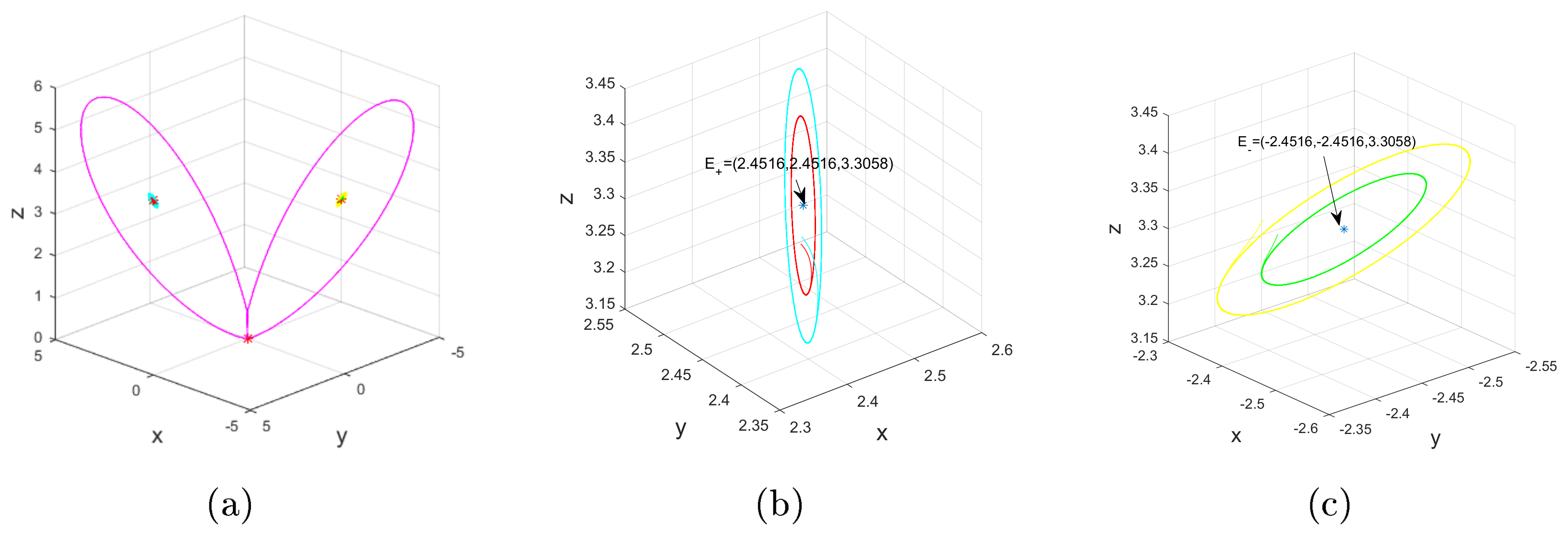
and Lemma 3 all lead to $h\in \{E_{-},E_0\}$. Therefore, $\mathsf{\Omega }\subseteq \{E_{-},E_0\}$. Because of the connectedness of $\mathsf{\Omega }$, the relation $\mathsf{\Omega }=E_{-}$ or $\mathsf{\Omega }=E_0$ holds. Based on Lemma 3 and Equation (14), one derives $\mathsf{\Omega }\ne E_0$. In a word, $\mathsf{\Omega }=E_{-}$, i.e., ${lim}_{n\to +\infty }{\psi }_{+}\left(t\right)=E_{-}$. Therefore, there exists a single heteroclinic orbit to $E_{-}$ and $E_0$. Due to the symmetry, there exists another unique heteroclinic orbit to $E_{+}$ and $E_0$ in system (1), as shown in Figure 8. The proof is finished. □

Figure 8. For $(a,c)=(6,100)$, $b=8,9$ and $(x_0^{1,3},y_0^{1,3},z_0^3)=(\pm 0.13,\pm 1.3,1.6)\times {10}^{-7}$, phase portraits of system (1), verifying the existence of a pair of heteroclinic orbits to unstable $E_0$ and stable $E_{\pm }$ when $c>0$ and $3b\ge 4a>0$.

5. Conclusions

Combining a theoretical analysis and numerical simulation, this paper investigates a newly reported 3D sub-quadratic four-thirds-degree Lorenz-like system, and reveals most of inherent dynamics of the Lorenz system family, i.e., self-excited attractors, Hopf bifurcation, generic and degenerate pitchfork, heteroclinic orbits, singularly degenerate heteroclinic cycle, an invariant algebraic surface, etc.

In contrast to the existing quadratic and sub-quadratic Lorenz-like analogues, we may find a new property: decreasing the powers of nonlinear terms may narrow and even eliminate the range of some certain parameters for hidden attractors, but enlarge it for self-excited attractors. This may verify the generalization of the second part of the celebrated Hilbert’s sixteenth problem to some degree: the number and mutual disposition of attractors and repellers may depend on the degree of polynomials of chaotic multidimensional dynamical systems. However, previous studies mainly emphasized that the aforementioned dynamics may explain the forming mechanism of strange attractors.

In future, we will expect other researchers to test this property through more Lorenz-like analogues, and clarify the relationship between other complex dynamics and the degrees, shedding light on the nature of chaos and providing reference for chaos-based applications.

References

- Smale, S. Mathematical problems for the next century. Math. Intell. 1998, 20, 7–15. [Google Scholar] [CrossRef]
- Lorenz, E.N. Deterministic nonperiodic flow. J. Atmos. Sci. 1963, 20, 130–141. [Google Scholar] [CrossRef]
- Afraimovich, V.S.; Bykov, V.V.; Shilnikov, L.P. The origin and structure of Lorenz attractor. Sov. Phys. Dokl. 1977, 22, 253–255. [Google Scholar]
- Tucker, W. The Lorenz attractor exists. Comptes Rendus l’Académie Sci. Ser. I Math. 1999, 328, 1197–1202. [Google Scholar] [CrossRef]
- Viana, M. What’s new on Lorenz strange attractors? Math. Intell. 2000, 22, 6–19. [Google Scholar] [CrossRef]
- Stewart, I. Mathematics: The Lorenz attractor exists. Nature 2000, 406, 948–949. [Google Scholar] [CrossRef] [PubMed]
- Shilnikov, L.P.; Shilnikov, A.L.; Turaev, D.V.; Chua, L.O. Methods of Qualitative Theory in Nonlinear Dynamics Part I, II; World Scientific: Singapore, 2001. [Google Scholar]
- Letellier, C.; Mendes, E.M.A.M.; Malasoma, J. Lorenz-like systems and Lorenz-like attractors: Definition, examples, and equivalences. Phys. Rev. E 2023, 108, 044209. [Google Scholar] [CrossRef]
- Kokubu, H.; Roussarie, R. Existence of a singularly degenerate heteroclinic cycle in the Lorenz system and its dynamical consequences: Part I. J. Dyn. Differ. Equ. 2004, 16, 513–557. [Google Scholar] [CrossRef]
- Messias, M. Dynamics at infinity and the existence of singularly degenerate heteroclinic cycles in the Lorenz system. J. Phys. A Math. Theor. 2009, 42, 115101. [Google Scholar] [CrossRef]
- Llibre, J.; Zhang, X. Invariant algebraic surfaces of the Lorenz system. J. Math. Phys. 2002, 43, 1622–1645. [Google Scholar] [CrossRef]
- Liao, X.; Yu, P.; Xie, S.; Fu, Y. Study on the global property of the smooth Chua’s system. Int. J. Bifurc. Chaos 2006, 16, 2815–2841. [Google Scholar] [CrossRef]
- Liao, X. New Research on Some Mathematical Problems of Lorenz Chaotic Family; Huazhong University of Science & Technology Press: Wuhan, China, 2017. [Google Scholar]
- Chen, G. Generalized Lorenz systems family. arXiv 2020, arXiv:2006.04066. [Google Scholar]
- Pasini, A.; Pelino, V. A unified view of Kolmogorov and Lorenz systems. Phys. Lett. A 2000, 275, 435–446. [Google Scholar] [CrossRef]
- Pelino, V.; Maimone, F.; Pasini, A. Energy cycle for the lorenz attractor. Chaos Solitons Fractals 2014, 64, 67–77. [Google Scholar] [CrossRef]
- Liang, X.; Qi, Q. Mechanical analysis of Chen chaotic system. Chaos Solitons Fractals 2017, 98, 173–177. [Google Scholar] [CrossRef]
- Leonov, G.A.; Kuznetsov, N.V. On differences and similarities in the analysis of Lorenz, Chen, and Lu systems. Appl. Math. Comput. 2015, 256, 334–343. [Google Scholar] [CrossRef]
- Kuznetsov, N.V.; Mokaev, T.N.; Kuznetsova, O.A.; Kudryashova, E.V. The Lorenz system: Hidden boundary of practical stability and the Lyapunov dimension. Nonlinear Dyn. 2020, 102, 713–732. [Google Scholar] [CrossRef]
- Zhang, X.; Chen, G. Constructing an autonomous system with infinitely many chaotic attractors. Chaos 2017, 27, 071101. [Google Scholar] [CrossRef]
- Liu, Y.; Yang, Q. Dynamics of a new Lorenz-like chaotic system. Nonl. Anal. RWA 2010, 11, 2563–2572. [Google Scholar] [CrossRef]
- Wang, H.; Ke, G.; Pan, J.; Hu, F.; Fan, H. Multitudinous potential hidden Lorenz-like attractors coined. Eur. Phys. J. Spec. Top. 2022, 231, 359–368. [Google Scholar] [CrossRef]
- Wang, H.; Pan, J.; Ke, G. Revealing more hidden attractors from a new sub-quadratic Lorenz-like system of degree . Int. J. Bifurc. Chaos 2024, 34, 2450071. [Google Scholar] [CrossRef]
- Sprott, J.C. A proposed standard for the publication of new chaotic systems. Int. J. Bifurc. Chaos 2011, 21, 2391–2394. [Google Scholar] [CrossRef]
- Llibre, J.; Messias, M.; Silva, P.R. On the global dynamics of the Rabinovich system. J. Phys. A Math. Theor. 2008, 41, 275210. [Google Scholar] [CrossRef]
- Wang, H.; Ke, G.; Pan, J.; Su, Q. Conjoined Lorenz-like attractors coined. Miskolc Math. Notes 2023. [Google Scholar]
- Ke, G. Creation of three-scroll hidden conservative Lorenz-like chaotic flows. Adv. Theory Simulations 2024. [Google Scholar] [CrossRef]
- Wang, H.; Ke, G.; Hu, F.; Pan, J.; Dong, G.; Chen, G. Pseudo and true singularly degenerate heteroclinic cycles of a new 3D cubic Lorenz-like system. Results Phys. 2024, 56, 107243. [Google Scholar] [CrossRef]
- Wang, H.; Pan, J.; Ke, G. Multitudinous potential homoclinic and heteroclinic orbits seized. Electron. Res. Arch. 2024, 32, 1003–1016. [Google Scholar] [CrossRef]
- Wang, H.; Pan, J.; Ke, G.; Hu, F. A pair of centro-symmetric heteroclinic orbits coined. Adv. Cont. Discr. Mod. 2024, 2024, 14. [Google Scholar] [CrossRef]
- Chen, Y.; Yang, Q. Dynamics of a hyperchaotic Lorenz-type system. Nonlinear Dyn. 2014, 77, 569–581. [Google Scholar] [CrossRef]
- Li, T.; Chen, G.; Chen, G. On homoclinic and heteroclinic orbits of the Chen’s system. Int. J. Bifurc. Chaos 2006, 16, 3035–3041. [Google Scholar] [CrossRef]
- Tigan, G.; Constantinescu, D. Heteroclinic orbits in the T and the Lü system. Chaos Solitons Fractals 2009, 42, 20–23. [Google Scholar] [CrossRef]
- Liu, Y.; Pang, W. Dynamics of the general Lorenz family. Nonlinear Dyn. 2012, 67, 1595–1611. [Google Scholar] [CrossRef]
- Tigan, G.; Llibre, J. Heteroclinic, homoclinic and closed orbits in the Chen system. Int. J. Bifurc. Chaos 2016, 26, 1650072. [Google Scholar] [CrossRef]
- Kuzenetsov, Y.A. Elements of Applied Bifurcation Theory, 3rd ed.; Springer: New York, NY, USA, 2004; Volume 112. [Google Scholar]
- Sotomayor, J.; Mello, L.F.; Braga, D.C. Lyapunov coefficients for degenerate Hopf bifurcations. arXiv 2007, arXiv:0709.3949. [Google Scholar]
Disclaimer/Publisher’s Note: The statements, opinions and data contained in all publications are solely those of the individual author(s) and contributor(s) and not of MDPI and/or the editor(s). MDPI and/or the editor(s) disclaim responsibility for any injury to people or property resulting from any ideas, methods, instructions or products referred to in the content. |
© 2024 by the authors. Licensee MDPI, Basel, Switzerland. This article is an open access article distributed under the terms and conditions of the Creative Commons Attribution (CC BY) license (https://creativecommons.org/licenses/by/4.0/).