On the Fractional Poisson Process and the Discretized Stable Subordinator

Abstract

We consider the renewal counting number process $N=N\left(t\right)$ as a forward march over the non-negative integers with independent identically distributed waiting times. We embed the values of the counting numbers N in a “pseudo-spatial” non-negative half-line $x\ge 0$ and observe that for physical time likewise we have $t\ge 0$. Thus we apply the Laplace transform with respect to both variables x and t. Applying then a modification of the Montroll-Weiss-Cox formalism of continuous time random walk we obtain the essential characteristics of a renewal process in the transform domain and, if we are lucky, also in the physical domain. The process $t=t\left(N\right)$ of accumulation of waiting times is inverse to the counting number process, in honour of the Danish mathematician and telecommunication engineer A.K. Erlang we call it the Erlang process. It yields the probability of exactly n renewal events in the interval $(0,t]$. We apply our Laplace-Laplace formalism to the fractional Poisson process whose waiting times are of Mittag-Leffler type and to a renewal process whose waiting times are of Wright type. The process of Mittag-Leffler type includes as a limiting case the classical Poisson process, the process of Wright type represents the discretized stable subordinator and a re-scaled version of it was used in our method of parametric subordination of time-space fractional diffusion processes. Properly rescaling the counting number process $N\left(t\right)$ and the Erlang process $t\left(N\right)$ yields as diffusion limits the inverse stable and the stable subordinator, respectively.

1. Introduction

Serious studies of the fractional generalization of the Poisson process—replacement of the exponential waiting time distribution by a distribution given via a Mittag-Leffler function with modified argument—have been started around the turn of the millenium, and since then many papers on its various aspects have appeared. There are in the literature many papers on this generalization where the authors have outlined a number of aspects and definitions, see e.g., Repin and Saichev (2000) [1], Wang et al. (2003,2006) [2,3], Laskin (2003,2009) [4,5], Mainardi et al. (2004) [6], Uchaikin et al. (2008) [7], Beghin and Orsingher (2009) [8], Cahoy et al. (2010) [9], Meerschaert et al. (2011) [10], Politi et al. (2011) [11], Kochubei (2012) [12], so that it seems impossible to list them all exhaustively. However, in effect this generalization was used already in 1995: Hilfer and Anton [13] (without saying it in our words) showed that the Fractional Kolmogorov-Feller equation (replacement of the first order time derivative by a fractional derivative of order between 0 and 1) requires the underlying random walk to be subordinated to a renewal process with Mittag-Leffler waiting time.

Here we will present our formalism for obtaining the essential characteristics of a generic renewal process and apply it to get those of the fractional Poisson counting process and its inverse, the fractional Erlang process. Both of these comprise as limiting cases the corresponding well-known non-fractional processes that are based on exponential waiting time. Then we will analyze an alternative renewal process, that we call the “Wright process”, investigated by Mainardi et al. (2000,2005,2007) [14,15,16], a process arising by discretization of the stable subordinator. In it the so-called M-Wright function plays the essential role. A scaled version of this process has been used by Barkai (2002) [17] for approximating the time-fractional diffusion process directly by a random walk subordinated to it (executing this scaled version in natural time), and he has found rather poor convergence in refinement. In Gorenflo et al. (2007) [18] we have modified the way of using this discretized stable subordinator. By appropriate discretization of the relevant spatial stable process we have then obtained a simulation method equivalent to the solution of a pair of Langevin equations, see Fogedby (1994) [19] and Kleinhans and Friedrich (2007) [20]. For simulation of space-time fractional diffusion one so obtains a sequence of precise snapshots of a true particle trajectory, see for details Gorenflo et al. (2007) [18], and also Gorenflo and Mainardi (2011, 2012) [21,22].

However, we should note that already in the Sixties of the past century, Gnedenko and Kovalenko (1968) [23] obtained in disguised form the fractional Poisson process by properly rescaled infinite thinning (rarefaction) of a renewal process with power law waiting time. By “disguised” we mean that they found the Laplace transform of the Mittag-Leffler waiting time density, but being ignorant of the Mittag-Leffler function they only presented this Laplace transform. The same ignorance of the Mittag-Leffler function we again meet in a 1985 paper by Balakrishnan [24], who exhibited the Mittag-Leffler waiting time density in Laplace disguise as essential for approximating time-fractional diffusion for which he used the description in form of a fractional integro-differential equation. We have shown that the Mittag-Leffler waiting time density in a certain sense is asymptotically universal for power law renewal processes, see Gorenflo and Mainardi (2008) [25], Gorenflo (2010) [26].

The structure of our paper is as follows. In Section 2 we discuss the elements of the general renewal theory and the CTRW concept. In Section 3 we introduce the Poisson process and its fractional generalization then, in Section 4, the so-called Wright process related to the stable subordinator and its discretization. For both processes we consider the corresponding inverse processes, the Erlang processes. In Section 5 we briefly discuss the diffusion limit for all the above processes. Section 6 is devoted to conclusions. We have collected in Appendix A notations and terminology, in particular the basics on operators, integral transforms and special functions required for understanding our analysis. Finally, we provide in Appendix B an overview on the essential results.

For related aspects of subordination we refer the readers to our papers [18,21,22,25,27] and to papers by Bazhlekova [28], by Merschaert’s team [10,29,30], and by Umarov [31].

2. Elements of Renewal Theory and CTRW

For the reader’s convenience let us here present a brief introduction to renewal theory including the basics of continuous time random walk (CTRW).

2.1. The General Renewal Process

By a renewal process we mean an infinite sequence $0=t_0<t_1<t_2<\cdots$ of events separated by i.i.d. (independent and identically distributed) random waiting times $T_j=t_j-t_{j-1}$, whose probability density $\mathsf{\varphi }\left(t\right)$ is given as a function or generalized function in the sense of Gel’fand and Shilov [32] (interpretable as a measure) with support on the positive real axis $t\ge 0$, non-negative: $\mathsf{\varphi }\left(t\right)\ge 0$, and normalized: ${\displaystyle {\int }_0^{\infty }\mathsf{\varphi }\left(t\right)dt}=1$, but not having a delta peak at the origin $t=0$. The instant $t_0=0$ is not counted as an event. An important global characteristic of a renewal process is its mean waiting time $⟨T⟩={\displaystyle {\int }_0^{\infty }t\mathsf{\varphi }\left(t\right)dt}$. It may be finite or infinite. In any renewal process we can distinguish two processes, namely the counting number process and the process inverse to it, that we call the Erlang process. The instants $t_1,t_2,t_3,\cdots$ are often called renewals. In fact renewal theory is relevant in practice of maintenance or required exchange of failed parts, e.g., light bulbs.

2.2. The Counting Number Process and Its Inverse

We are interested in the counting number process $x=N=N\left(t\right)$

$$N\left(t\right):=\text{max}\left\{n|t_n\le t\right\}=n\text{for}{t}_n\le t<t_{n+1},n=0,1,2,\cdots$$

(2.1)

where in particular $N\left(0\right)=0$. We ask for the counting number probabilities in n, evolving in t,

$$p_n\left(t\right):=\mathcal{P}[N\left(t\right)=n],n=0,1,2,\cdots$$

(2.2)

We denote by $p(x,t)$ the sojourn density for the counting number having the value x. For this process the expectation is

$$m\left(t\right):=⟨N\left(t\right)⟩=\sum _{n=0}^{\infty }n{p}_n\left(t\right)={\int }_0^{\infty }xp(x,t)dx$$

(2.3)

[since $p(x,t)={\displaystyle \sum _{n=0}^{\infty }{p}_n\left(t\right)\mathsf{\delta }(x-n)}$, see (2.12)] It provides the mean number of events in the half-open interval $(0,t]$, and is called the renewal function, see e.g., [33]. We also will look at the process $t=t\left(N\right)$, the inverse to the process $N=N\left(t\right)$, that we call the Erlang process in honour of the Danish telecommunication engineer A.K. Erlang (1878–1929), see Brockmeyer et al. (1948) [34]. It gives the value of time $t=t_N$ of the N-th renewal. We ask for the Erlang probability densities

$$q_n\left(t\right)=q(t,n),n=0,1,2,\dots$$

(2.4)

For every n the function $q_n\left(t\right)=q(t,n)$ is a density in the variable of time having value t in the instant of the n-th event. Clearly, this event occurs after n (original) waiting times have passed, so that

$$q_n\left(t\right)={\mathsf{\varphi }}^{*n}\left(t\right)\text{with}\text{Laplace}\text{transform}{\tilde{q}}_n\left(s\right)=\left(\tilde{\mathsf{\varphi }}{\left(s\right)}^n\right)$$

(2.5)

In other words the function $q_n\left(t\right)=q(t,n)$ is a probability density in the variable $t\ge 0$ evolving in the variable $x=n=0,1,2,...$.

2.3. The Continuous time Random Walk

A continuous time random walk (CTRW) is given by an infinite sequence of spatial positions $0=x_0,x_1,x_2,\cdots$, separated by (i.i.d.) random jumps $X_j=x_j-x_{j-1}$, whose probability density function $w\left(x\right)$ is given as a non-negative function or generalized function (interpretable as a measure) with support on the real axis $-\infty <x<+\infty$ and normalized: ${\displaystyle {\int }_0^{\infty }w\left(x\right)dx}=1$, this random walk being subordinated to a renewal process so that we have a random process $x=x\left(t\right)$ on the real axis with the property $x\left(t\right)=x_n$ for $t_n\le t<t_{n+1}$, $n=0,1,2,\cdots$.

We ask for the sojourn probability density $u(x,t)$ of a particle wandering according to the random process $x=x\left(t\right)$ being in point x at instant t.

Let us define the following cumulative probabilities related to the probability density function $\mathsf{\varphi }\left(t\right)$

$$\mathsf{\Phi }\left(t\right)={\int }_0^{t+}\mathsf{\varphi }\left(t^{\prime }\right)d{t}^{\prime },\mathsf{\Psi }\left(t\right)={\int }_{t+}^{\infty }\mathsf{\varphi }\left(t^{\prime }\right)d{t}^{\prime }=1-\mathsf{\Phi }\left(t\right)$$

(2.6)

For definiteness, we take $\mathsf{\Phi }\left(t\right)$ as right-continuous, $\mathsf{\Psi }\left(t\right)$ as left-continuous. When the non-negative random variable represents the lifetime of a technical system, it is common to call $\mathsf{\Phi }\left(t\right):=\mathcal{P}\left(T\le t\right)$ the failure probability and $\mathsf{\Psi }\left(t\right):=\mathcal{P}\left(T>t\right)$ the survival probability, because $\mathsf{\Phi }\left(t\right)$ and $\mathsf{\Psi }\left(t\right)$ are the respective probabilities that the system does or does not fail in $(0,t]$. These terms, however, are commonly adopted for any renewal process.

In the Fourier-Laplace domain we have

$$\tilde{\mathsf{\Psi }}\left(s\right)=\frac{1-\tilde{\mathsf{\varphi }}\left(s\right)}{s}$$

(2.7)

and the famous Montroll-Weiss solution formula for a CTRW, see [35,36]

$$\widehat{\tilde{u}}(\mathsf{\kappa },s)={\displaystyle \frac{1-\tilde{\mathsf{\varphi }}\left(s\right)}{s}\sum _{n=0}^{\infty }{\left(\tilde{\mathsf{\varphi }}\left(s\right)\widehat{w}\left(\mathsf{\kappa }\right)\right)}^n}={\displaystyle \frac{1-\tilde{\mathsf{\varphi }}\left(s\right)}{s}\frac{1}{1-\tilde{\mathsf{\varphi }}\left(s\right)\widehat{w}\left(\mathsf{\kappa }\right)}}$$

(2.8)

In our special situation the jump density has support only on the positive semi-axis $x\ge 0$ and thus, by replacing the space-Fourier transform $\widehat{w}\left(\mathsf{\kappa }\right)$ with the space-Laplace transform $\tilde{w}\left(\mathsf{\kappa }\right)$, we obtain from (2.8) the Laplace-Laplace solution that we re-write as a new equation

$$\tilde{\tilde{u}}(\mathsf{\kappa },s)={\displaystyle \frac{1-\tilde{\mathsf{\varphi }}\left(s\right)}{s}\sum _{n=0}^{\infty }{\left(\tilde{\mathsf{\varphi }}\left(s\right)\tilde{w}\left(\mathsf{\kappa }\right)\right)}^n}{\displaystyle =\frac{1-\tilde{\mathsf{\varphi }}\left(s\right)}{s}\frac{1}{1-\tilde{\mathsf{\varphi }}\left(s\right)\tilde{w}\left(\mathsf{\kappa }\right)}}$$

(2.9)

Recalling from Appendix the definition of convolutions, in the physical domain we have for the solution $u(x,t)$ the Cox-Weiss series, see [36,37],

$$u(x,t)=\left(\mathsf{\Psi }*\sum _{n=0}^{\infty }{\mathsf{\varphi }}^{*n}{w}^{*n}\right)(x,t)$$

(2.10)

This formula has an intuitive meaning: Up to and including instant t, there have occurred 0 jumps, or 1 jump, or 2 jumps, or ⋯, and if the last jump has occurred at instant $t^{\prime }<t$, the wanderer is resting there for a duration $t-t^{\prime }$.

From the rich literature on the concept of CTRW and its applications we recommend to study the surveys by Metzler and Klafter [38,39] and the original article by Chechkin, Hofmann and Sokolov [40].

2.4. Renewal Process as a Special CTRW

The essential trick of what follows consists in a rather non-conventional use of the CTRW concept. We treat renewal processes as continuous time random walks with waiting time density $\mathsf{\varphi }\left(t\right)$ and special jump density $w\left(x\right)=\mathsf{\delta }(x-1)$ corresponding to the fact that the counting number $N\left(t\right)$ increases by 1 at each positive event instant $t_n$. We then have $\tilde{w}\left(\mathsf{\kappa }\right)=\exp (-\mathsf{\kappa })$ and get for the counting number process $N\left(t\right)$ the sojourn density in the transform domain ($s\ge 0$, $\mathsf{\kappa }\ge 0$),

$$\tilde{\tilde{p}}(\mathsf{\kappa },s)={\displaystyle \frac{1-\tilde{\mathsf{\varphi }}\left(s\right)}{s}\sum _{n=0}^{\infty }{\left(\tilde{\mathsf{\varphi }}\left(s\right)\right)}^n{\mathrm{e}}^{-n\mathsf{\kappa }}}={\displaystyle \frac{1-\tilde{\mathsf{\varphi }}\left(s\right)}{s}\frac{1}{1-\tilde{\mathsf{\varphi }}\left(s\right){\mathrm{e}}^{-\mathsf{\kappa }}}}$$

(2.11)

From this formula we can find formulas for the renewal function $m\left(t\right)$ and the probabilities $p_n\left(t\right)=P\{N\left(t\right)=n\}$. Because $N\left(t\right)$ assumes as values only the non-negative integers, the sojourn density $p(x,t)$ vanishes if x is not equal to one of these, but has a delta peak of height $p_n\left(t\right)$ for $x=n$ ($n=0,1,2,3,\cdots$). Hence

$$p(x,t)=\sum _{n=0}^{\infty }{p}_n\left(t\right)\mathsf{\delta }(x-n)$$

(2.12)

Inverting (2.11) with respect to κ and s as

$$p(x,t)=\sum _{n=0}^{\infty }\left(\mathsf{\Psi }*{\mathsf{\varphi }}^{*n}\right)\left(t\right)\mathsf{\delta }(x-n)$$

(2.13)

we identify

$$p_n\left(t\right)=\left(\mathsf{\Psi }*{\mathsf{\varphi }}^{*n}\right)\left(t\right)$$

(2.14)

According to the theory of Laplace transform we conclude from Equations (2.2) and (2.12)

$$m\left(t\right)={\displaystyle -\frac{\partial }{\partial \mathsf{\kappa }}{\left.\tilde{p}(\mathsf{\kappa },t)\right|}_{\mathsf{\kappa }=0}}={\displaystyle {\left.\left(\sum _{n=0}^{\infty }n{p}_n\left(t\right){\mathrm{e}}^{-n\mathsf{\kappa }}\right)\right|}_{\mathsf{\kappa }=0}}={\displaystyle \sum _{n=0}^{\infty }n{p}_n\left(t\right)}$$

(2.15)

a result naturally expected, and

$$\tilde{m}\left(s\right)={\displaystyle \sum _{n=0}^{\infty }n{\tilde{p}}_n\left(s\right)}={\displaystyle \tilde{\mathsf{\Psi }}\left(s\right)\sum _{n=0}^{\infty }n{\left(\tilde{\mathsf{\varphi }}\left(s\right)\right)}^n}={\displaystyle \frac{\tilde{\mathsf{\varphi }}\left(s\right)}{s\left(1-\tilde{\mathsf{\varphi }}\left(s\right)\right)}}$$

(2.16)

thereby using the identity

$$\sum _{n=0}^{\infty }n{z}^n=\frac{z}{{(1-z)}^2},\left|z\right|<1$$

Thus we have found in the Laplace domain the reciprocal pair of relationships

$$\tilde{m}\left(s\right)=\frac{\tilde{\mathsf{\varphi }}\left(s\right)}{s(1-\tilde{\mathsf{\varphi }}\left(s\right))},\tilde{\mathsf{\varphi }}\left(s\right)=\frac{s\tilde{m}\left(s\right)}{1+s\tilde{m}\left(s\right))}$$

(2.17)

saying that the waiting time density and the renewal function mutually determine each other uniquely. The first formula of Equation (2.17) can also be obtained as the value at $\mathsf{\kappa }=0$ of the negative derivative for $\mathsf{\kappa }=0$ of the last expression in Equation (2.11). Equation (2.17) implies the reciprocal pair of relationships in the physical domain

$$m\left(t\right)={\int }_0^t[1+m(t-t^{\prime })]\mathsf{\varphi }\left(t^{\prime }\right)d{t}^{\prime },m^{\prime }\left(t\right)={\int }_0^t[1+m^{\prime }(t-t^{\prime })]\mathsf{\varphi }\left(t^{\prime }\right)d{t}^{\prime }$$

(2.18)

The first of these equations usually is called the renewal equation.

Considering, formally, the counting number process $N=N\left(t\right)$ as CTRW (with jumps fixed to unit jumps 1), N running increasingly through the non-negative integers $x=0,1,2,...$, happening in natural time $t\in [0,\infty )$, we note that in the Erlang process $t=t\left(N\right)$, the roles of N and t are interchanged. The new “waiting time density” now is $w\left(x\right)=\mathsf{\delta }(x-1)$, the new “jump density” is $\mathsf{\varphi }\left(t\right)$.

It is illuminating to consciously perceive the relationships for $t\ge 0$, $n=0,1,2,\dots$, between the counting number probabilities $p_n\left(t\right)$ and the Erlang densities $q_n\left(t\right)$. For Equation (2.5) we have $q_n\left(t\right)={\mathsf{\varphi }}^{*n}\left(t\right)$, and then by (2.14)

$$p_n\left(t\right)=\left(\mathsf{\Psi }*q_n\right)\left(t\right)={\int }_0^t\left(q_n\left(t^{\prime }\right)-q_{n+1}\left(t\right)\right)d{t}^{\prime }$$

(2.19)

We can also express the $q_n$ in another way by the $p_n$. Introducing the cumulative probabilities $Q_n\left(t\right)={\displaystyle {\int }_0^t{q}_n\left(t^{\prime }\right)d{t}^{\prime }}$, we have

$$Q_n\left(t\right)=\mathcal{P}\left(\sum _{k=1}^n{T}_k\le t\right)=\mathcal{P}\left(N\left(t\right)\ge n\right)=\sum _{k=n}^{\infty }{p}_k\left(t\right)$$

(2.20)

finally

$$q_n\left(t\right)=\frac{d}{dt}{Q}_n\left(t\right)=\frac{d}{dt}\sum _{k=n}^{\infty }{p}_k\left(t\right)$$

(2.21)

All this is true for $n=0$ as‘well, by the empty sum convention ${\displaystyle \sum _{k=1}^n{T}_k}=0$ for $n=0$.

3. The Poisson Process and Its Fractional Generalization

The most popular renewal process is the Poisson process. It is (uniquely) characterized by its mean waiting time $1/\mathsf{\lambda }$ (equivalently by its intensity λ), which is a given positive number, and by its residual waiting time $\mathsf{\Psi }\left(t\right)=\exp (-\mathsf{\lambda }t)$ for $t\ge 0$, which corresponds to the waiting time density $\mathsf{\varphi }\left(t\right)=\mathsf{\lambda }\exp (-\mathsf{\lambda }t)$. With $\mathsf{\lambda }=1$ we have what we call the standard Poisson process. The general Poisson process arises from the standard one by rescaling the time variable t.

We generalize the standard Poisson process by replacing the exponential function by a function of Mittag-Leffler type. With $t\ge 0$ and a parameter $\mathsf{\beta }\in (0,1]$ we take

$$\left\{\begin{array}{cc}\mathsf{\Psi }\left(t\right)\hfill & =E_{\mathsf{\beta }}(-t^{\mathsf{\beta }}),\hfill \\ \mathsf{\varphi }\left(t\right)\hfill & =-{\displaystyle \frac{d}{dt}}{E}_{\mathsf{\beta }}(-t^{\mathsf{\beta }})=\mathsf{\beta }{t}^{\mathsf{\beta }-1}{E}_{\mathsf{\beta }}^{\prime }(-t^{\mathsf{\beta }})=t^{\mathsf{\beta }-1}{E}_{\mathsf{\beta },\mathsf{\beta }}(-t^{\mathsf{\beta }})\hfill \end{array}\right.$$

(3.1)

The functions $\mathsf{\Psi }\left(t\right)$ and $\varphi \left(t\right)$ are plotted versus time for some values of β in Figure 1.

Figure 1. The functions $\mathsf{\Psi }\left(t\right)$ (left) and $\mathsf{\varphi }\left(t\right)$ (right) versus t (${10}^{-2}<t<{10}^2$) for the renewal processes of Mittag-Leffler type with $\mathsf{\beta }=0.25,0.50,0.75,1$.

Figure 1. The functions $\mathsf{\Psi }\left(t\right)$ (left) and $\mathsf{\varphi }\left(t\right)$ (right) versus t (${10}^{-2}<t<{10}^2$) for the renewal processes of Mittag-Leffler type with $\mathsf{\beta }=0.25,0.50,0.75,1$.

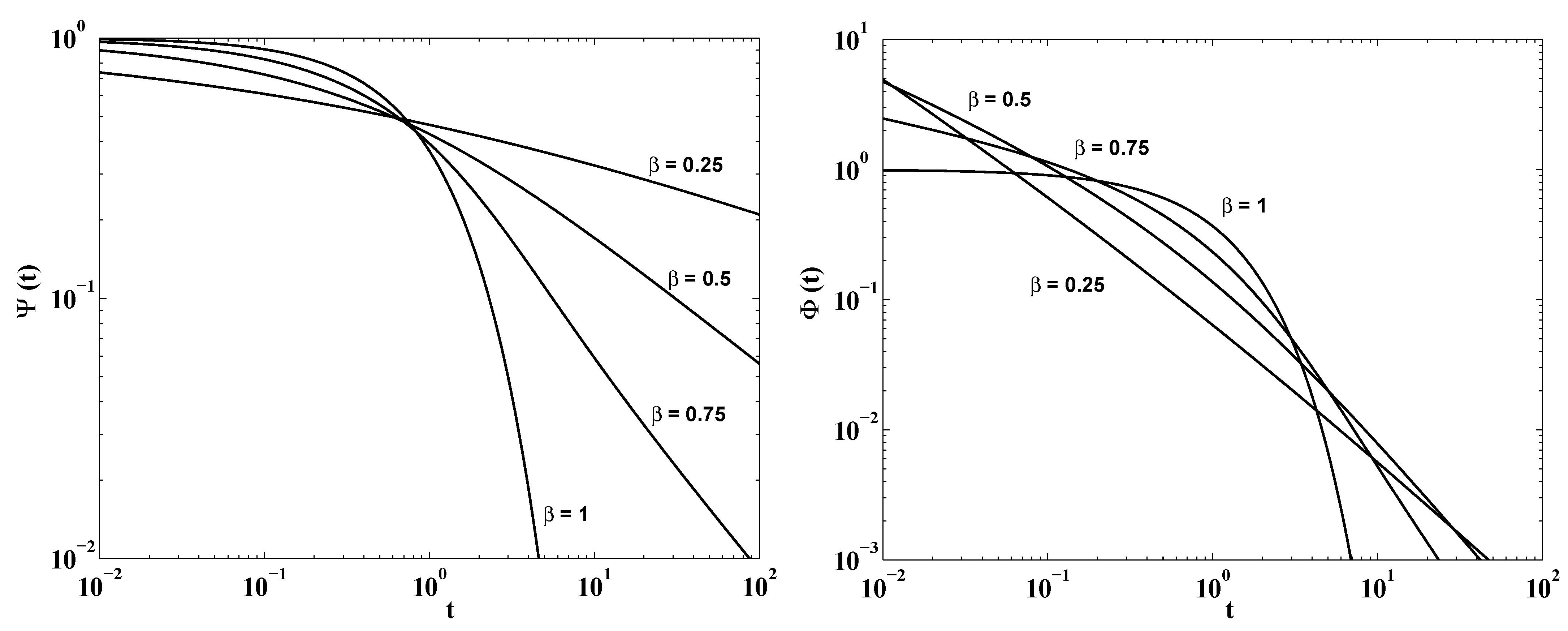
We call this renewal process of Mittag-Leffler type the fractional Poisson process, see e.g., [1,4,6,8,9,10,11,27,41,42], and [7,43], or the Mittag-Leffler renewal process or the Mittag-Leffler waiting time process.

To analyze it we go into the Laplace domain where we have

$$\tilde{\mathsf{\Psi }}\left(s\right)=\frac{s^{\mathsf{\beta }-1}}{1+s^{\mathsf{\beta }}},\tilde{\mathsf{\varphi }}\left(s\right)=\frac{1}{1+s^{\mathsf{\beta }}}$$

(3.2)

If there is no danger of misunderstanding we will not decorate Ψ and $\mathsf{\varphi }$ with the index β. The special choice $\mathsf{\beta }=1$ gives us the standard Poisson process with ${\mathsf{\Psi }}_1\left(t\right)={\mathsf{\varphi }}_1\left(t\right)=\exp (-t)$.

Whereas the Poisson process has finite mean waiting time (that of its standard version is equal to 1), the fractional Poisson process ($0<\mathsf{\beta }<1$ ) does not have this property. In fact,

$$⟨T⟩={\int }_0^{\infty }t\mathsf{\varphi }\left(t\right)dt=\mathsf{\beta }{\left.{\displaystyle \frac{s^{\mathsf{\beta }-1}}{{(1+s^{\mathsf{\beta }})}^2}}\right|}_{s=0}=\left\{\begin{array}{cc}1,\hfill & \mathsf{\beta }=1,\hfill \\ \infty ,\hfill & 0<\mathsf{\beta }<1.\hfill \end{array}\right.$$

(3.3)

Let us calculate the renewal function $m\left(t\right)$. Inserting $\tilde{\mathsf{\varphi }}\left(s\right)=1/(1+s^{\mathsf{\beta }})$ into Equation (2.11) and taking $w\left(x\right)=\mathsf{\delta }(x-1)$ as in Section 2, we find for the sojourn density of the counting function $N\left(t\right)$ the expressions

$$\tilde{\tilde{p}}(\mathsf{\kappa },s)=\frac{s^{\mathsf{\beta }-1}}{1+s^{\mathsf{\beta }}-{\mathrm{e}}^{-\mathsf{\kappa }}}=\frac{s^{\mathsf{\beta }-1}}{1+s^{\mathsf{\beta }}}\sum _{n=0}^{\infty }\frac{{\mathrm{e}}^{-n\mathsf{\kappa }}}{{(1+s^{\mathsf{\beta }})}^n}$$

(3.4)

and

$$\tilde{p}(\mathsf{\kappa },t)=E_{\mathsf{\beta }}\left(-(1-{\mathrm{e}}^{-\mathsf{\kappa }})t^{\mathsf{\beta }}\right)$$

(3.5)

and then

$$m\left(t\right)=-\frac{\partial }{\partial \mathsf{\kappa }}{\left.\tilde{p}(\mathsf{\kappa },t)\right|}_{\mathsf{\kappa }=0}={\left.{\mathrm{e}}^{-\mathsf{\kappa }}{t}^{\mathsf{\beta }}{E}_{\mathsf{\beta }}^{\prime }\left(-(1-{\mathrm{e}}^{-\mathsf{\kappa }})t^{\mathsf{\beta }}\right)\right|}_{\mathsf{\kappa }=0}$$

(3.6)

Using $E_{\mathsf{\beta }}^{\prime }\left(0\right)=1/\Gamma (1+\mathsf{\beta })$ now yields

$$m\left(t\right)=\left\{\begin{array}{cc}t,\hfill & \mathsf{\beta }=1\hfill \\ {\displaystyle \frac{t^{\mathsf{\beta }}}{\Gamma (1+\mathsf{\beta })}},\hfill & 0<\mathsf{\beta }<1\hfill \end{array}\right.$$

(3.7)

This result can also be obtained by plugging $\tilde{\mathsf{\varphi }}\left(s\right)=1/(1+s^{\mathsf{\beta }})$ into the first equation in (2.17) which yields $\tilde{m}\left(s\right)=1/s^{\mathsf{\beta }+1}$ and then by Laplace inversion Equation (3.7).

Using general Taylor expansion

$$E_{\mathsf{\beta }}\left(z\right)=\sum _{n=0}^{\infty }\frac{E_{\mathsf{\beta }}^{\left(n\right)}}{n!}{(z-b)}^n$$

(3.8)

in Equation (3.5) with $b=-t^{\mathsf{\beta }}$ we get

$$\begin{array}{cc}\tilde{p}(\mathsf{\kappa },t)\hfill & ={\displaystyle \sum _{n=0}^{\infty }\frac{t^{n\mathsf{\beta }}}{n!}{E}_{\mathsf{\beta }}^{\left(n\right)}(-t^{\mathsf{\beta }}){\mathrm{e}}^{-n\mathsf{\kappa }}}\hfill \\ p(x,t)\hfill & ={\displaystyle \sum _{n=0}^{\infty }\frac{t^{n\mathsf{\beta }}}{n!}{E}_{\mathsf{\beta }}^{\left(n\right)}(-t^{\mathsf{\beta }})\mathsf{\delta }(x-n)}\hfill \end{array}$$

(3.9)

and, by comparison with Equation (2.12), the counting number probabilities

$$p_n\left(t\right)=\mathcal{P}\{N\left(t\right)=n\}=\frac{t^{n\mathsf{\beta }}}{n!}{E}_{\mathsf{\beta }}^{\left(n\right)}(-t^{\mathsf{\beta }})$$

(3.10)

Observing from Equation (3.4)

$$\tilde{\tilde{p}}(\mathsf{\kappa },s)=\frac{s^{\mathsf{\beta }-1}}{1+s^{\mathsf{\beta }}}\sum _{n=0}^{\infty }\frac{{\mathrm{e}}^{-n\mathsf{\kappa }}}{{(1+s^{\mathsf{\beta }})}^n}$$

(3.11)

and inverting with respect to κ,

$$\tilde{p}(x,s)=\frac{s^{\mathsf{\beta }-1}}{1+s^{\mathsf{\beta }}}\sum _{n=0}^{\infty }\frac{\mathsf{\delta }(x-n)}{{(1+s^{\mathsf{\beta }})}^n}$$

(3.12)

we finally identify

$${\tilde{p}}_n\left(s\right)=\frac{s^{\mathsf{\beta }-1}}{{(1+s^{\mathsf{\beta }})}^{n+1}}÷\frac{t^{n\mathsf{\beta }}}{n!}{E}_{\mathsf{\beta }}^{\left(n\right)}(-t^{\mathsf{\beta }})=p_n\left(t\right)$$

(3.13)

En passant we have proved an often cited special case of an inversion formula by Podlubny (1999) [44], Equation (1.80).

For the Poisson process with intensity $\mathsf{\lambda }>0$ we have a well-known infinite system of ordinary differential equations (for $t\ge 0$), see e.g., Khintchine [45,46],

$$p_0\left(t\right)={\mathrm{e}}^{-\mathsf{\lambda }t},\frac{d}{dt}{p}_n\left(t\right)=\mathsf{\lambda }\left(p_{n-1}\left(t\right)-p_n\left(t\right)\right),n\ge 1$$

(3.14)

with initial conditions $p_n\left(0\right)=0$, $n=1,2,\cdots$, which sometimes even is used to define the Poisson process. We have an analogous system of fractional differential equations for the fractional Poisson process. In fact, from Equation (3.13) we have

$$(1+s^{\mathsf{\beta }}){\tilde{p}}_n\left(s\right)=\frac{s^{\mathsf{\beta }-1}}{{(1+s^{\mathsf{\beta }})}^n}={\tilde{p}}_{n-1}\left(s\right)$$

(3.15)

Hence

$$s^{\mathsf{\beta }}{\tilde{p}}_n\left(s\right)={\tilde{p}}_{n-1}\left(s\right)-{\tilde{p}}_n\left(s\right)$$

(3.16)

so in the time domain

$$p_0\left(t\right)=E_{\mathsf{\beta }}(-t^{\mathsf{\beta }}),{}_{*}{D}_t^{\mathsf{\beta }}{p}_n\left(t\right)=p_{n-1}\left(t\right)-p_n\left(t\right),n\ge 1$$

(3.17)

with initial conditions $p_n\left(0\right)=0$, $n=1,2,\cdots$, where ${}_{*}{D}_t^{\mathsf{\beta }}$ denotes the time-fractional derivative of Caputo type of order β, see Appendix A. It is also possible to introduce and define the fractional Poisson process by this difference-differential system.

Let us note that by solving the system (3.17), Beghin and Orsingher in [8] introduce what they call the “first form of the fractional Poisson process”, and in [10] Meerschaert et al. show that this process is a renewal process with Mittag-Leffler waiting time density as in (3.1), hence is identical with the fractional Poisson process.

Up to now we have investigated the fractional Poisson counting process $N=N\left(t\right)$ and found its probabilities $p_n\left(t\right)$ in Equation (3.10). To get the corresponding Erlang probability densities $q_n\left(t\right)=q(t,n)$, densities in t, evolving in $n=0,1,2\dots$, we find by Equation (2.21) via telescope summation

$$q_n\left(t\right)=\mathsf{\beta }\frac{t^{n\mathsf{\beta }-1}}{(n-1)!}{E}_{\mathsf{\beta }}^{\left(n\right)}\left(-t^{\mathsf{\beta }}\right),0<\mathsf{\beta }\le 1$$

(3.18)

We leave it as an exercise to the readers to show that in Equation (3.9) interchange of differentiation and summation is allowed.

Remark: With $\mathsf{\beta }=1$ we get the corresponding well-known results for the standard Poisson process. The counting number probabilities are

$$p_n\left(t\right)=\frac{t^n}{n!}{\mathrm{e}}^{-t},n=0,1,2,\dots ,t\ge 0$$

(3.19)

and the Erlang densities

$$q_n\left(t\right)=\frac{t^{n-1}}{(n-1)!}{\mathrm{e}}^{-t},n=1,2,3,\dots ,,t\ge 0$$

(3.20)

By rescalation of time we obtain

$$p_n\left(t\right)=\frac{{\left(\mathsf{\lambda }t\right)}^n}{n!}{\mathrm{e}}^{-\mathsf{\lambda }t},n=0,1,2,\dots ,,t\ge 0$$

(3.21)

for the classical Poisson process with intensity λ and

$$q_n\left(t\right)=\mathsf{\lambda }\frac{{\left(\mathsf{\lambda }t\right)}^{n-1}}{(n-1)!}{\mathrm{e}}^{-\mathsf{\lambda }t},n=1,2,3,\dots ,,t\ge 0$$

(3.22)

for the corresponding Erlang process.

4. The Stable Subordinator and the Wright Process

Let us denote by $g_{\mathsf{\beta }}\left(t\right)$ the extremal Lévy stable density of order $\mathsf{\beta }\in (0,1]$ and support in $t\ge 0$ whose Laplace transform is ${\tilde{g}}_{\mathsf{\beta }}\left(s\right)=\exp (-s^{\mathsf{\beta }})$, that is

$$t\ge 0,g_{\mathsf{\beta }}\left(t\right)÷\exp (-s^{\mathsf{\beta }}),Re\left(s\right)\ge 0,0<\mathsf{\beta }\le 1$$

(4.1)

The topic of Lévy stable distributions is treated in several books on probability and stochastic processes, see e.g., Feller (1971) [47], Sato (1999) [48]; an overview of the analytical and graphical aspects of the corresponding densities is found in Mainardi et al. (2001) [49], where an ad hoc notation is used.

From the Laplace transform correspondence (4.1) it is easy to derive the analytical expressions for $\mathsf{\beta }=1/2$ (the so-called Lévy-Smirmov density), $g_{1/2}\left(t\right)={\displaystyle \frac{1}{2\sqrt{\pi }}{t}^{-3/2}\exp (-1/\left(4t\right))}$ and for the limiting case $\mathsf{\beta }=1$ (the time drift), $g_1\left(t\right)=\mathsf{\delta }(t-1)$, where δ denotes the Dirac generalized function.

We note that the stable density (4.1) can be expressed in terms of a function of the Wright type. In fact, with the M-Wright function from Appendix A of this paper (see Appendix F of Mainardi’s book [50] for more details), we have

$$g_{\mathsf{\beta }}\left(t\right)=\frac{\mathsf{\beta }}{t^{\mathsf{\beta }+1}}{M}_{\mathsf{\beta }}\left(t^{-\mathsf{\beta }}\right)$$

(4.2)

The renewal process with waiting time density

$$\mathsf{\varphi }\left(t\right)=g_{\mathsf{\beta }}\left(t\right)$$

(4.3)

was considered in detail by Mainardi et al. (2000,2005,2007) [14,15,16]. We call this process the Wright renewal process because the corresponding survival function $\mathsf{\Psi }\left(t\right)$ and the waiting time density $\mathsf{\varphi }\left(t\right)$ are expressed in terms of certain Wright functions. So we distinguish it from the so called Mittag-Leffler renewal process, treated in the previous Section as fractional Poisson process. More precisely, recalling the Wright functions from the Appendix A, we have for $t\ge 0$,

$$\mathsf{\Psi }\left(t\right)=\left\{\begin{array}{cc}1-W_{-\mathsf{\beta },1}\left(-\frac{1}{t^{\mathsf{\beta }}}\right),\hfill & 0<\mathsf{\beta }<1,\hfill \\ \Theta \left(t\right)-\Theta (t-1),\hfill & \mathsf{\beta }=1,\hfill \end{array}\right.\text{from}\tilde{\mathsf{\Psi }}\left(s\right)=\frac{1-{\mathrm{e}}^{{\displaystyle -s^{\mathsf{\beta }}}}}{s}$$

(4.4)

$$\mathsf{\varphi }\left(t\right)=\left\{\begin{array}{cc}\frac{1}{t}{W}_{-\mathsf{\beta },0}\left(-\frac{1}{t^{\mathsf{\beta }}}\right),\hfill & 0<\mathsf{\beta }<1,\hfill \\ \mathsf{\delta }(t-1),\hfill & \mathsf{\beta }=1,\hfill \end{array}\right.\text{from}\tilde{\mathsf{\varphi }}\left(s\right)={\mathrm{e}}^{{\displaystyle -s^{\mathsf{\beta }}}}$$

(4.5)

where Θ denotes the unit step Heaviside function. The functions $\mathsf{\Psi }\left(t\right)$ and $\varphi \left(t\right)$ are plotted versus time for some values of β in Figure 2.

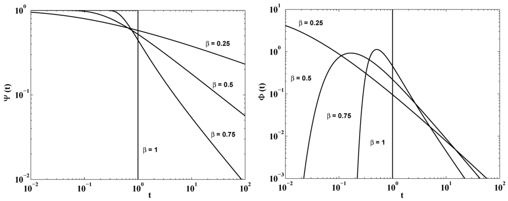
Figure 2. The functions $\mathsf{\Psi }\left(t\right)$ (left) and $\mathsf{\varphi }\left(t\right)$ (right) versus t (${10}^{-2}<t<{10}^2$) for the renewal processes of Wright type with $\mathsf{\beta }=0.25,0.50,0.75,1$. For $\mathsf{\beta }=1$ the reader would recognize the Box function (extended up to $t=1$) at left and the delta function (centred in $t=1$) at right.

Figure 2. The functions $\mathsf{\Psi }\left(t\right)$ (left) and $\mathsf{\varphi }\left(t\right)$ (right) versus t (${10}^{-2}<t<{10}^2$) for the renewal processes of Wright type with $\mathsf{\beta }=0.25,0.50,0.75,1$. For $\mathsf{\beta }=1$ the reader would recognize the Box function (extended up to $t=1$) at left and the delta function (centred in $t=1$) at right.

It is relevant to note the Laplace transform connecting the two transcendental functions $M_{\mathsf{\beta }}$ and $E_{\mathsf{\beta }}$

$$M_{\mathsf{\beta }}\left(t\right)÷E_{\mathsf{\beta }}(-s),0<\mathsf{\beta }\le 1$$

(4.6)

By the stable subordinator of order $\mathsf{\beta }\in (0,1]$ we mean the stochastic process $t=t\left(x\right)$ that has sojourn density in $t\ge 0$, evolving in $x\ge 0$ provided by the Laplace transform correspondence,

$$\tilde{f}(s,x)={\mathrm{e}}^{{\displaystyle -x{s}^{\mathsf{\beta }}}}÷f(t,x)=x^{-1/\mathsf{\beta }}{g}_{\mathsf{\beta }}\left(x^{-1/\mathsf{\beta }}t\right)=\frac{\mathsf{\beta }}{t^{\mathsf{\beta }+1}}{x}^{1+1/\mathsf{\beta }}{M}_{\mathsf{\beta }}\left(x{t}^{-\mathsf{\beta }}\right)$$

(4.7)

This process is monotonically increasing: for this reason it is used in the context of time change and subordination in fractional diffusion processes.

We discretize the process $t=t\left(x\right)$ by restricting x to run through the integers $n=0,1,2,\dots$. The resulting discretized version is a renewal process happening in pseudo-time $x\ge 0$ with jumps in pseudo-space $t\ge 0$ having density $g_{\mathsf{\beta }}\left(t\right)$. Inverting this discretized stable subordinator we obtain a counting number process $x=N=N\left(t\right)$ with waiting time density and jump density

$$\mathsf{\varphi }\left(t\right)=g_{\mathsf{\beta }}\left(t\right),w\left(x\right)=\mathsf{\delta }(x-1)$$

(4.8)

Because here the waiting time density is given by a function of Wright type we call this process the Wright renewal process, or simply the Wright process. Immediately we get its Erlang densities (in $t\ge 0$, evolving in $x=n=0,1,2,\dots$)

$$q_n\left(t\right)={\mathsf{\varphi }}^{*n}\left(t\right)÷{\mathrm{e}}^{-n{s}^{\mathsf{\beta }}}$$

(4.9)

so that, in view of (4.7) with $x=n$,

$$q_n\left(t\right)=f(t,n)=n^{-1/\mathsf{\beta }}{g}_{\mathsf{\beta }}\left(n^{-1/\mathsf{\beta }}t\right)$$

(4.10)

In the special case $\mathsf{\beta }=1$ we have $q_n\left(t\right)=\mathsf{\delta }(t-n)$.

We observe that this counting process gives us precise snapshots at $x=0,1,2,$ of the stable subordinator $t=t\left(x\right)$.

Using (4.9) in (2.14) we find the counting number probabilities in time and Laplace domain

$$p_n\left(t\right)=(\mathsf{\Psi }*{\mathsf{\varphi }}^{*n})\left(t\right)÷{\tilde{p}}_n\left(s\right)={\displaystyle \frac{1-{\mathrm{e}}^{-s^{\mathsf{\beta }}}}{s}{\mathrm{e}}^{-n{s}^{\mathsf{\beta }}}}={\displaystyle \frac{{\mathrm{e}}^{-n{s}^{\mathsf{\beta }}}-{\mathrm{e}}^{-(n+1)s^{\mathsf{\beta }}}}{s}}$$

(4.11)

hence

$$p_n\left(t\right)={\int }_0^t\left(q_n\left(t^{\prime }\right)-q_{n+1}\left(t^{\prime }\right)\right)d{t}^{\prime }$$

(4.12)

according to (2.19).

With the probability distribution function

$$G_{\mathsf{\beta }}\left(t\right)={\int }_0^t{g}_{\mathsf{\beta }}\left(t^{\prime }\right)d{t}^{\prime }$$

(4.13)

we get

$$p_n\left(t\right)=G_{\mathsf{\beta }}\left(n^{-1/\mathsf{\beta }}t\right)-G_{\mathsf{\beta }}\left({(n+1)}^{-1/\mathsf{\beta }}t\right)$$

(4.14)

In the limiting case $\mathsf{\beta }=1$ we have

$$G_1\left(t\right)={\int }_0^t\mathsf{\delta }(t^{\prime }-1)d{t}^{\prime }=\left\{\begin{array}{cc}0\hfill & \text{for}t<1\hfill \\ 1\hfill & \text{for}t\ge 1\hfill \end{array}\right.$$

(4.15)

as a function continuous from the right, and we calculate

$$p_n\left(t\right)=\left\{\begin{array}{cc}0\hfill & \text{for}0<t<n,\text{and}\text{for}t\ge n+1\hfill \\ 1\hfill & \text{for}n\le t<n+1\hfill \end{array}\right.$$

(4.16)

For the renewal function we obtain its Laplace transform from (2.17)

$$\tilde{m}\left(s\right)=\frac{{\mathrm{e}}^{-s^{\mathsf{\beta }}}}{s(1-{\mathrm{e}}^{-s^{\mathsf{\beta }}})}=\frac{1}{s}\sum _{n=1}^{\infty }{\mathrm{e}}^{-n{s}^{\mathsf{\beta }}}$$

(4.17)

so that

$$m\left(t\right)=\sum _{n=1}^{\infty }{\int }_0^t{q}_n\left(t^{\prime }\right)d{t}^{\prime }=\sum _{n=1}^{\infty }{G}_{\mathsf{\beta }}\left(n^{-1/\mathsf{\beta }}t\right)$$

(4.18)

We do not know an explicit expression for this sum if $0<\mathsf{\beta }<1$. However, in the limiting case $\mathsf{\beta }=1$ we obtain

$$m\left(t\right)=\left[t\right]=N\left(t\right)$$

(4.19)

Using (4.17) we investigate the asymptotic behaviour of $m\left(t\right)$ for $t\to \infty$. We have for $s\to 0$ $\tilde{m}\left(s\right)\sim 1/s^{1+\mathsf{\beta }}$ and thus, by Tauber theory, see e.g., Feller (1971) [47],

$$m\left(t\right)\sim \frac{t^{\mathsf{\beta }}}{\Gamma (1+\mathsf{\beta })}\text{for}t\to \infty$$

(4.20)

Remember, for the fractional Poisson process, we had found

$$m\left(t\right)=\frac{t^{\mathsf{\beta }}}{\Gamma (1+\mathsf{\beta })}\text{for}\text{all}t\ge 0(4.21)$$

(4.21)

Remark: A rescaled version of the discretized stable subordinator can be used for producing closely spaced precise snapshots of a true particle trajectory of a space-time fractional diffusion process, see e.g., the recent chapter by Gorenflo and Mainardi (2011) [22] on parametric subordination.

5. The Diffusion Limits for the Fractional Poisson and the Wright Processes

In a CTRW we can, with positive scaling factor h and τ, replace the jumps X by jumps $X_h=hX$, the waiting times T by waiting times $T_{\mathsf{\tau }}=\mathsf{\tau }T$. This leads to the rescaled jump density $w_h\left(x\right)=w(x/h)/h$ and the rescaled waiting time density ${\mathsf{\varphi }}_{\mathsf{\tau }}\left(t\right)=\mathsf{\varphi }(t/\mathsf{\tau })/\mathsf{\tau }$ and correspondingly to the transforms ${\widehat{w}}_h\left(\mathsf{\kappa }\right)=\widehat{w}\left(h\mathsf{\kappa }\right)$, ${\tilde{\mathsf{\varphi }}}_{\mathsf{\tau }}\left(s\right)=\tilde{\mathsf{\varphi }}\left(\mathsf{\tau }s\right)$.

For the sojourn density $u_{h,\mathsf{\tau }}(x,t)$, density in x evolving in t, we obtain from (2.9) in the transform domain

$${\widehat{\tilde{u}}}_{h,\mathsf{\tau }}(\mathsf{\kappa },s)=\frac{1-\tilde{\mathsf{\varphi }}\left(\mathsf{\tau }s\right)}{s}\frac{1}{1-\tilde{\mathsf{\varphi }}\left(\mathsf{\tau }s\right)\widehat{w}\left(h\mathsf{\kappa }\right)}$$

(5.1)

where, if $w\left(x\right)$ has support on $x\ge 0$ we can work with the Laplace transform instead of the Fourier transform (replace the $\widehat{\phantom{x}}$ by $\tilde{\phantom{x}}$). If there exists between h and τ a scaling relation $\mathcal{R}$ (to be introduced later) under which $u(x,t)$ tends for $h\to 0$, $\mathsf{\tau }\to 0$ to a meaningful limit $v(x,t)=u_{0,0}(x,t)$, then we call the process $x=x\left(t\right)$ with this sojourn density a diffusion limit. We find it via

$$\widehat{\tilde{v}}(\mathsf{\kappa },s)=\underset{h,\mathsf{\tau }\to 0\left(\mathcal{R}\right)}{lim}{\widehat{\tilde{u}}}_{h,\mathsf{\tau }}(\mathsf{\kappa },s)$$

(5.2)

and Fourier-Laplace (or Laplace-Laplace) inversion.

Remark: This diffusion limit is a limit in the weak sense (convergence in distribution of the CTRW to the diffusion limit). The mathematical background consists in the application of the Fourier (or Laplace) continuity theorem of probability theory for fixed time t.

We will now find that the counting numbers of the fractional Poisson process and the Wright process have the same diffusion limit, namely the inverse stable subordinator. The two corresponding Erlang processes have the same diffusion limit, namely the stable subordinator. For $t\to \infty$ the renewal functions have the same asymptotic behaviour, namely $m\left(t\right)\sim t^{\mathsf{\beta }}/\Gamma (1+\mathsf{\beta })$. Here, in the case of the fractional Poisson process, we can replace the sign ∼ of asymptotics by the sign = of equality for all $t\ge 0$.

To prove these statements we need the Laplace transform of the relevant functions $\mathsf{\varphi }\left(t\right)$ and $w\left(x\right)$. For the fractional Poisson process we have

$$\mathsf{\varphi }\left(t\right)=\frac{d}{dt}{E}_{\mathsf{\beta }}(-t^{\mathsf{\beta }})÷\tilde{\mathsf{\varphi }}\left(s\right)=\frac{1}{1+s^{\mathsf{\beta }}},w\left(x\right)=\mathsf{\delta }(x-1)÷\tilde{w}\left(\mathsf{\kappa }\right)=\exp (-\mathsf{\kappa })$$

For the Wright process we have

$$\mathsf{\varphi }\left(t\right)=g_{\mathsf{\beta }}\left(t\right)÷\tilde{\mathsf{\varphi }}\left(s\right)=\exp (-s^{\mathsf{\beta }}),w\left(x\right)=\mathsf{\delta }(x-1)÷\tilde{w}\left(\mathsf{\kappa }\right)=\exp (-\mathsf{\kappa })$$

In all cases we have, for fixed s and κ

$$\tilde{\mathsf{\varphi }}\left(\mathsf{\tau }s\right)\sim 1-{\left(\mathsf{\tau }s\right)}^{\mathsf{\beta }}\text{as}\mathsf{\tau }\to 0,\tilde{w}\left(h\mathsf{\kappa }\right)\sim 1-\left(h\mathsf{\kappa }\right)\text{as}h\to 0,$$

and straightforwardly we obtain for the sojourn densities in both cases, by use of (5.1) with p in place of u and $\widehat{\phantom{x}}$ replaced by $\tilde{\phantom{x}}$

$${\tilde{\tilde{p}}}_{h,\mathsf{\tau }}(\mathsf{\kappa },s)\sim \frac{{\mathsf{\tau }}^{\mathsf{\beta }}{s}^{\mathsf{\beta }-1}}{{\mathsf{\tau }}^{\mathsf{\beta }}{s}^{\mathsf{\beta }}+h\mathsf{\kappa }},\text{for}\mathsf{\tau }\to 0,h\to 0$$

(5.3)

Using the scaling relation $\mathcal{R}$

$$h={\mathsf{\tau }}^{\mathsf{\beta }}$$

(5.4)

we obtain

$${\tilde{\tilde{p}}}_{0,0}(\mathsf{\kappa },s)=\frac{s^{\mathsf{\beta }-1}}{s^{\mathsf{\beta }}+\mathsf{\kappa }}$$

(5.5)

By partial Laplace inversions we get two equivalent representations

$$p_{0,0}(x,t)={\mathcal{L}}_{\mathsf{\kappa }}^{-1}\left\{E_{\mathsf{\beta }}(-\mathsf{\kappa }{t}^{\mathsf{\beta }})\right\}={\mathcal{L}}_s^{-1}\left\{s^{\mathsf{\beta }-1}\exp (-x{s}^{\mathsf{\beta }})\right\}$$

(5.6)

leading to the density of the inverse stable subordinator

$$p_{0,0}(x,t)=t^{-\mathsf{\beta }}{M}_{\mathsf{\beta }}(x/t^{\mathsf{\beta }})=J_t^{1-\mathsf{\beta }}f(t,x)$$

(5.7)

where $M_{\mathsf{\beta }}$ and $J_t^{1-\mathsf{\beta }}$ denote respectively the M-Wright function and the Riemann-Liouville fractional integral introduced in Appendix A, and $f(t,x)$ the stable subordinator given by Equation (4.7).

Remark: In (4.7) and (5.7) the densities of the stable and the inverse stable subordinator are both represented via the M-Wright function.

The Diffusion Limit for the Erlang Process

In the Erlang process the roles of space and time, likewise of jumps and waiting times, are interchanged. In other words we treat $x\ge 0$ as a pseudo-time variable and $t\ge 0$ as a pseudo-space variable. For the resulting sojourn density $q(t,x)$, we have from interchanging in (5.1) for $h\to 0$ and $\mathsf{\tau }\to 0$,

$${\tilde{\tilde{q}}}_{h,\mathsf{\tau }}(s,\mathsf{\kappa })=\frac{1-\tilde{w}\left(h\mathsf{\kappa }\right)}{k}\frac{1}{1-\tilde{w}\left(h\mathsf{\kappa }\right)\tilde{\mathsf{\varphi }}\left(\mathsf{\tau }s\right)}\sim \frac{h}{h\mathsf{\kappa }+{\left(\mathsf{\tau }s\right)}^{\mathsf{\beta }}}$$

(5.8)

Again using the scaling relation $\mathcal{R}$ in Equation (5.4) we find

$${\tilde{\tilde{q}}}_{0,0}(s,\mathsf{\kappa })=\frac{1}{\mathsf{\kappa }+s^{\mathsf{\beta }}},$$

(5.5´)

which is the Laplace-Laplace transform of the density of stable subordinator of Section 4. In fact, by partial Laplace inversion,

$${\tilde{q}}_{0,0}(s,x)=\exp (-x{s}^{\mathsf{\beta }})=\tilde{f}(s,x),$$

(5.9)

and it follows that

$$q_{0,0}(t,x)=f(t,x),x\ge 0,t\ge 0.$$

(5.10)

See (4.7) for its explicit representation as a rescaled stable density expressed via a M-Wright function.

We get the same result by continualization of the discretized stable subordinator. Replace in Equations (4.9) and (4.10) the discrete variable n by the continuous variable x.

6. Conclusions

The fractional Poisson process and the Wright process (as discretization of the stable subordinator) along with their diffusion limits play eminent roles in theory and simulation of fractional diffusion processes. Here we have analyzed these two processes, concretely the corresponding counting number and Erlang processes, the latter being the processes inverse to the former. Furthermore we have obtained the diffusion limits of all these processes by well-scaled refinement of waiting times and jumps.

References

- Repin, O.N.; Saichev, A.I. Fractional Poisson law. Radiophys. Quantum Electron. 2000, 43, 738–741. [Google Scholar] [CrossRef]
- Wang, X.; Wen, Z. Poisson fractional processes. Chaos Solitons Fractals 2003, 18, 169–177. [Google Scholar] [CrossRef]
- Wang, X.; Wen, Z.; Zhang, S. Fractional Poisson process (II). Chaos Solitons Fractals 2006, 28, 143–147. [Google Scholar] [CrossRef]
- Laskin, N. Fractional Poisson process. Commun. Nonlinear Sci. Numer. Simul. 2003, 8, 201–213. [Google Scholar] [CrossRef]
- Laskin, N. Some applications of the fractional Poisson probability distribution. J. Math. Phys. 2009, 50, 113513:1–113513:12. [Google Scholar] [CrossRef]
- Mainardi, F.; Gorenflo, R.; Scalas, E. A fractional generalization of the Poisson processes. Vietnam J. Math. 2004, 32, 53–64. Available online: http://arxiv.org/abs/math/0701454 (accessed on 3 August 2015). [Google Scholar]
- Uchaikin, V.V.; Cahoy, D.O.; Sibatov, R.T. Fractional processes: From Poisson to branching one. Int. J. Bifurcation Chaos 2008, 18, 1–9. [Google Scholar] [CrossRef]
- Beghin, L.; Orsingher, E. Fractional Poisson processes and related random motions. Electron. Journ. Prob. 2009, 14, 1790–1826. [Google Scholar] [CrossRef]
- Cahoy, D.O.; Uchaikin, V.V.; Woyczynski, W.A. Parameter estimation for fractional Poisson processes. J. Stat. Plan. Inference 2010, 140, 3106–3120. [Google Scholar] [CrossRef]
- Meerschaert, M.M.; Nane, E.; Vellaisamy, P. The fractional Poisson process and the inverse stable subordinator. Electron. J. Prob. 2011, 16, 1600–1620. Available online: http://arxiv.org/abs/1007.505 (accessed on 3 August 2015). [Google Scholar] [CrossRef]
- Politi, M.; Kaizoji, T.; Scalas, E. Full characterization of the fractional Poisson process. Eur. Phys. Lett. 2011, 96, 20004:1–20004:6. [Google Scholar] [CrossRef]
- Kochubei, A.N. General fractional calculus, evolution equations, and renewal processes. Integral Equ. Oper. Theory 2011, 71, 583–600. Available online: http://arxiv.org/abs/1105.1239 (accessed on 3 August 2015). [Google Scholar] [CrossRef]
- Hilfer, H.; Anton, L. Fractional master equations and fractal time random walks. Phys. Rev. E 1995, 51, R848–R851. [Google Scholar] [CrossRef]
- Mainardi, F.; Raberto, M.; Gorenflo, R.; Scalas, E. Fractional calculus and continuous-time finance II: The waiting-time distribution. Phys. A 2000, 287, 468–481. Available online: http://arxiv.org/abs/cond-mat/0006454 (accessed on 3 August 2015). [Google Scholar] [CrossRef]
- Mainardi, F.; Gorenflo, R.; Vivoli, A. Renewal processes of Mittag-Leffler and Wright type. Fract. Calc. Appl. Anal. 2005, 8, 7–38. Available online: http://arxiv.org/abs/math/0701455 (accessed on 3 August 2015). [Google Scholar]
- Mainardi, F.; Gorenflo, R.; Vivoli, A. Beyond the Poisson renewal process: A tutorial survey. J. Comp. Appl. Math 2007, 205, 725–735. [Google Scholar] [CrossRef]
- Barkai, E. CTRW pathways to the fractional diffusion equation. Chem. Phys. 2002, 284, 13–27. [Google Scholar] [CrossRef]
- Gorenflo, R.; Mainardi, F.; Vivoli, A. Continuous time random walk and parametric subordination in fractional diffusion. Chaos Solitons Fractals 2007, 34, 87–103. Available online: http://arxiv.org/abs/cond-mat/0701126 (accessed on 3 August 2015). [Google Scholar] [CrossRef]
- Fogedby, H.C. Langevin equations for continuous time Lévy flights. Phys. Rev. E 1994, 50, 1657–1660. [Google Scholar] [CrossRef]
- Kleinhans, D.; Friedrich, R. Continuous-time random walks: Simulations of continuous trajectories. Phys. Rev E 2007, 76, 061102:1–061102:6. [Google Scholar] [CrossRef] [PubMed]
- Gorenflo, R.; Mainardi, F. Subordination pathways to fractional diffusion. Eur. Phys. J. Spec. Top. 2011, 193, 119–132. Available online: http://arxiv.org/abs/1104.4041 (accessed on 3 August 2015). [Google Scholar] [CrossRef]
- Gorenflo, R.; Mainardi, F. Parametric Subordination in Fractional Diffusion Processes. In Fractional Dynamics; Klafter, J., Lim, S.C., Metzler, R., Eds.; World Scientific: Singapore, 2012; Chapter 10; pp. 229–263. Available online: http://arxiv.org/abs/1210.8414 (accessed on 3 August 2015).
- Gnedenko, B.V.; Kovalenko, I.N. Introduction to Queueing Theory; Israel Program for Scientific Translations: Jerusalem, Israel, 1968. [Google Scholar]
- Balakrishnan, V. Anomalous diffusion in one dimension. Phys. A 1985, 132, 569–580. [Google Scholar] [CrossRef]
- Gorenflo, R.; Mainardi, F. Continuous time random walk, Mittag-Leffler waiting time and fractional diffusion: Mathematical aspects. In Anomalous Transport: Foundations and Applications; Klages, R., Radons, G., Sokolov, I.M., Eds.; Wiley-VCH: Weinheim, Germany, 2008; Chapter 4; pp. 93–127. Available online: http://arxiv.org/abs/0705.0797 (accessed on 3 August 2015).
- Gorenflo, R. Mittag-Leffler waiting time, power laws, rarefaction, continuous time random walk, diffusion limit. In Proceedings of the National Workshop on Fractional Calculus and Statistical Distributions, CMS Pala Campus, India, 25–27 November 2010; Pai, S.S., Sebastian, N., Nair, S.S., Joseph, D.P., Kumar, D., Eds.; pp. 1–22. Available online: http://arxiv.org/abs/1004.4413 (accessed on 3 August 2015).
- Gorenflo, R.; Mainardi, F. Laplace-Laplace analysis of the fractional Poisson process. In Analytical Methods of Analysis and Differential Equations; Rogosin, S., Ed.; Belarusan State University: Minsk, Belarus, 2012; Kilbas Memorial Volume, pp. 43–58. Available online: http://arxiv.org/abs/1305.5473 (accessed on 3 August 2015).
- Bazhlekova, E. Subordination principle for a class of fractional order differential equations. Mathematics 2015, 2, 412–427. [Google Scholar] [CrossRef]
- Meerschaert, M.M. Fractional Calculus, Anomalous Diffusion, and Probability. In Fractional Dynamics; Lim, S.C., Klafter, J., Metzler, R., Eds.; World Scientific: Singapore, 2012; Chapter 11; pp. 265–284. [Google Scholar]
- Meerschaert, M.M.; Benson, D.A.; Scheffler, H.-P.; Baeumer, B. Stochastic solution of space-time fractional diffusion equations. Phys. Rev. E 2002, 65, 41103:1–41103:4. [Google Scholar] [CrossRef] [PubMed]
- Umarov, S. Continuous time random walk models for fractional space-time diffusion equations. Fract. Calc. Appl. Anal. 2015, 18, 821–837. [Google Scholar] [CrossRef]
- Gel’fand, I.M.; Shilov, G.E. Generalized Functions; Academic Press: New York, NY, USA, 1964; Volume 1. [Google Scholar]
- Ross, S.M. Stochastic Processes, 2nd ed.; Wiley: New York, NY, USA, 1996. [Google Scholar]
- Brockmeyer, E.; Halstrøm, H.L.; Jensen, A. The Life and Works of A.K. Erlang, Transactions of the Danish Academy of Technical Sciences, No 2; The Copenhagen Telephone Company: Copenhagen, Denmark, 1948. [Google Scholar]
- Montroll, E.W.; Weiss, G.H. Random walks on lattices, II. J. Math. Phys. 1965, 6, 167–181. [Google Scholar] [CrossRef]
- Weiss, G.H. Aspects and Applications of Random Walks; North-Holland: Amsterdam, The Netherlands, 1994. [Google Scholar]
- Cox, D.R. Renewal Theory, 2nd ed.; Methuen: London, UK, 1967. [Google Scholar]
- Metzler, R.; Klafter, J. The random walker’s guide to anomalous diffusion: A fractional dynamics approach. Phys. Rep. 2000, 339, 1–77. [Google Scholar] [CrossRef]
- Metzler, R.; Klafter, J. The restaurant at the end of the random walk: Recent developments in the description of anomalous transport by fractional dynamics. J. Phys. A. Math. Gen. 2004, 37, R161–R208. [Google Scholar] [CrossRef]
- Chechkin, A.V.; Hofmann, M.; Sokolov, I.M. Continuous-time random walk with correlated waiting times. Phys. Rev. E 2009, 80. [Google Scholar] [CrossRef] [PubMed]
- Baleanu, D.; Diethelm, K.; Scalas, E.; Trujillo, J.J. Fractional Calculus: Models and Numerical Methods; World Scientific: Singapore, 2012. [Google Scholar]
- Scalas, E. A class of CTRWs: Compound fractional Poisson processes. In Fractional Dynamics; Klafter, J., Lim, S.C., Metzler, R., Eds.; World Scientific: Singapore, 2012; Chapter 15; pp. 353–374. [Google Scholar]
- Uchaikin, V.V. Fractional Derivatives for Physicists and Engineers, Vol. I, Background and Theory; Springer: Heidelberg, Germany, 2013. [Google Scholar]
- Podlubny, I. Fractional Differential Equations; Academic Press: San Diego, CA, USA, 1999. [Google Scholar]
- Khintchine, A.Y. Mathematical Methods in the Theory of Queuing; Charles Griffin: London, UK, 1960. [Google Scholar]
- Rogosin, S.V.; Mainardi, F. The Legacy of A.Ya. Khintchine’s Work in Probability Theory; Cambridge Scientific Publ.: Cambridge, UK, 2011; Available online: http://www.cambridgescientificpublishers.com/ (accessed on 3 August 2015).
- Feller, W. An Introduction to Probability Theory and its Applications; Wiley: New York, NY, USA, 1971; Volume II. [Google Scholar]
- Sato, K.-I. Lévy Processes and Infinitely Divisible Distributions; Cambridge University Press: Cambridge, UK, 1999. [Google Scholar]
- Mainardi, F.; Luchko, Y.; Pagnini, G. The fundamental solution of the space-time fractional diffusion equation. Fract. Calc. Appl. Anal. 2001, 4, 153–192. [Google Scholar]
- Mainardi, F. Fractional Calculus and Waves in Linear Viscoelasticity; Imperial College Press: London, UK, 2010. [Google Scholar]
- Gorenflo, R.; Abdel-Rehim, E. From power laws to fractional diffusion: The direct way. Vietnam J. Math. 2004, 32, 65–75. [Google Scholar]
- Gorenflo, R.; Mainardi, F. Fractional calculus: Integral and differential equations of fractional order. In Fractals and Fractional Calculus in Continuum Mechanics; Carpinteri, A., Mainardi, F., Eds.; Springer Verlag: Wien, Austria, 1997; pp. 223–276. Available online: http://arxiv.org/abs/0805.3823 (accessed on 3 August 2015).
- Gorenflo, R.; Mainardi, F.; Scalas, E.; Raberto, M. Fractional calculus and continuous-time finance III: The diffusion limit. In Mathematical Finance; Kohlmann, M., Tang, S., Eds.; Birkhäuser Verlag: Basel, Swizerland, 2001; pp. 171–180. [Google Scholar]
- Mainardi, F.; Mura, A.; Pagnini, G. The M-Wright function in time-fractional diffusion processes: A tutorial survey. Int. J. Diff. Equ. 2010, 2010, 104505:1–104505:29. Available online: http://arxiv.org/abs/1004.2950 (accessed on 3 August 2015). [Google Scholar] [CrossRef]
- Scalas, E.; Gorenflo, R.; Mainardi, F. Fractional calculus and continuous-time finance. Phys. A 2000, 284, 376–384. Available online: http://arxiv.org/abs/cond-mat/0001120 (accessed on 3 August 2015). [Google Scholar] [CrossRef]
- Scalas, E.; Gorenflo, R.; Mainardi, F. Uncoupled continuous-time random walks: Solution and limiting behavior of the master equation. Phys. Rev. E 2004, 69, 011107:1–011107:8. [Google Scholar] [CrossRef] [PubMed]
- Gorenflo, R.; Kilbas, A.A.; Mainardi, F.; Rogosin, S.V. Mittag-Leffler Functions, Related Topics and Applications; Springer: Heidelberg, Germany, 2014. [Google Scholar]
- Kilbas, A.A.; Saigo, M. H-Transform: Theory and Applications; Chapman and Hall/CRC: New York, NY, USA, 2004. [Google Scholar]
- Kilbas, A.A.; Srivastava, H.M.; Trujillo, J.J. Theory and Applications of Fractional Differential Equations; Elsevier: Amsterdam, The Netherlands, 2006. [Google Scholar]
- Mathai, A.M.; Haubold, H.J. Special Functions for Applied Scientists; Springer: New York, NY, USA, 2008. [Google Scholar]
- Mathai, A.M.; Saxena, R.K.; Haubold, H.J. The H-function, Theory and Applications; Springer Verlag: New York, NY, USA, 2010. [Google Scholar]
- Diethelm, K. The Analysis of Fractional Differential Equations. An Application Oriented Exposition Using Differential Operators of Caputo Type; Springer: Berlin, Germany, 2010. [Google Scholar]
- Atanacković, T.M.; Pilipović, S.; Stanković, B.; Zorica, D. Fractional Calculus with Applications in Mechanics: Vibrations and Diffusion Processes; ISTE Ltd, London and John Wiley: Hoboken, NJ, USA, 2014. [Google Scholar]
- Haubold, H.J.; Mathai, A.M.; Saxena, R.K. Mittag-Leffler functions and their applications. J. Appl. Math. 2011, 2011, 298628:1–298628:51. [Google Scholar] [CrossRef]
- Abramowitz, M.; Stegun, I.A. Handbook of Mathematical Functions; Dover: New York, NY, USA, 1965. [Google Scholar]
© 2015 by the authors; licensee MDPI, Basel, Switzerland. This article is an open access article distributed under the terms and conditions of the Creative Commons Attribution license (http://creativecommons.org/licenses/by/4.0/).