A New gH-Difference for Multi-Dimensional Convex Sets and Convex Fuzzy Sets

Abstract

In the setting of Minkowski set-valued operations, we study generalizations of the difference for (multidimensional) compact convex sets and for fuzzy sets on metric vector spaces, extending the Hukuhara difference. The proposed difference always exists and allows defining Pompeiu-Hausdorff distance for the space of compact convex sets in terms of a pseudo-norm, i.e., the magnitude of the difference set. A computational procedure for two dimensional sets is outlined and some examples of the new difference are given.

1. Introduction

It is well-known that in interval and set-valued arithmetic, the standard addition $A+B=\{a+b|a\in A,b\in B\}$ is not an invertible operation and in particular the algebraic difference $A-B=\{a-b|a\in A,b\in B\}$ is such that $A-A\ne 0$. The interval case has been analyzed and solved by several authors since the 1970s, in the setting of interval analysis. In particular, S. Markov proposed an extended interval arithmetic, including a difference (inner difference ${-}^{-}$) with the basic property that $A{-}^{-}A=0$ and a division (inner division ${:}^{-}$) such that $A{:}^{-}A=1$ (see [1,2,3,4]).

The same problem applies to the general case of (nonempty) compact convex sets in ${\mathbb{R}}^n$: finding a difference operation as an inverse of Minkowski addition $A+B$ of compact convex sets has been a field of long interest; well-known and largely used examples are: the Hukuhara difference, proposed in [5], but it exists only in specific cases; the geometric Pontryagin difference, proposed in [6], but it may be the empty set; the Demyanov difference, introduced in the setting of subdifferential calculus and nonsmooth analysis (see, e.g., [7,8,9,10,11]).

The Hukuhara difference has been recently generalized in [12], in the setting of fuzzy arithmetic, with applications to differentiability of fuzzy-valued functions of a single variable (see [13,14,15]) and multiple variables (see [16]).

Two other approaches have been proposed in the setting of set-valued analysis: in [17,18,19,20]) directed sets are used; and in [21], the difference of A and B is expressed in terms of minimal pairs $(A^{\prime },B^{\prime })$ of compact convex sets such that $A+A^{\prime }=B+B^{\prime }$ (using the Radstrom embedding theorem [22,23]).

On the other hand, inversion of addition is important in set-valued and fuzzy arithmetic and analysis, with many applications e.g., in solving equations and differential equations (for recent results and other references to the fuzzy case, see e.g., [13,14,24,25,26,27,28,29,30,31,32,33,34]).

Extending the results in [12,14], we define a generalized difference for general compact convex sets and we extend it to fuzzy sets with compact and convex $\alpha$-cuts. The multidimensional fuzzy case has been addressed only occasionally and by very few papers in the literature; some basic results on the gH-difference for multidimensional intervals (boxes) were obtained in [12] and recently used by [35] in the study of fuzzy vector-valued functions.

The new proposed difference, as we will see, is not unique in the general case; but this is not necessarily a negative aspect: we can add specific requirements to select particular difference sets with additional properties, depending on the application at hand, or we can take the union (or the convexified union) of the existing difference sets obtaining a set with the same properties.

For the convex case, efficient computational procedures are suggested and illustrated for convex sets in ${\mathbb{R}}^2$. Some of the results contained in this paper have been presented at the 2016 Joint Mathematics Meetings of the AMS Mathematical Association of America (January 6–9, 2016, Seattle, WA). Procedures for the approximation of the new difference in ${\mathbb{R}}^n$ are presented in [36].

The paper is organized as follows. Section 2 introduces some preliminary concepts for compact convex sets and fuzzy sets. Section 3 introduces the new generalized difference for compact convex sets and analyses some of its basic properties. Section 4 presents computational methods and examples in two dimensions. In Section 5 we extend the new difference to the fuzzy case and in Section 6 we conclude with an outline of possible applications.

2. The Space of Compact Convex Sets

Consider the metric vector space ${\mathbb{R}}^n$, $n\ge 1$, of real vectors, equipped with standard addition and scalar multiplication operations. Following Diamond and Kloeden (see [37], with applications in [38,39]), denote by ${\mathcal{K}}_C\left({\mathbb{R}}^n\right)$ the space of nonempty compact convex sets of ${\mathbb{R}}^n$.

Given two subsets $A,B\in {\mathcal{K}}_C\left({\mathbb{R}}^n\right)$ and $k\in \mathbb{R}$, Minkowski addition and scalar multiplication are defined by $A+B=\{a+b|a\in A,b\in B\}$ and $kA=\left\{ka\right|a\in A\}$ and it is well-known that addition is associative and commutative and with neutral element $\left\{0\right\}$. The following properties are well-known ([40]):

$$\begin{array}{ccc}\hfill (A\cup B)+C& =& (A+C)\cup (B+C)\hfill \\ \hfill (A\cap B)+C& \subseteq & (A+C)\cap (B+C)\hfill \\ \hfill A\cup B\mathrm{convex}& \Rightarrow & (A\cap B)+C=(A+C)\cap (B+C).\hfill \end{array}$$

For brevity, we will indicate by 0 the neutral element $\left\{0\right\}$.

A subtraction for two sets $A,B\in {\mathcal{K}}_C\left({\mathbb{R}}^n\right)$ can be defined, according to standard Minkowski operations, by $A-B=$$A+(-1)B=$$\{a-b|a\in A,b\in B\}$ and, in general, even when the cancellation law $(A+C=B+C)\iff A=B$ is valid, addition/subtraction simplification is not valid, i.e., $A-A\ne 0$ and $(A+B)-B\ne A$.

For sets $A,B\in {\mathcal{K}}_C\left({\mathbb{R}}^n\right)$ in a normed space $({\mathbb{R}}^n,||·|\left|\right)$, the Pompeiu-Hausdorff distance is defined as usual by

$$d_H(A,B)=max\{d_{*}(A,B),d_{*}(B,A)\}$$

(1)

where

$$d_{*}(A,B)=\underset{a\in A}{sup}\underset{b\in B}{inf}∥a-b∥\mathrm{and}{d}_{*}(B,A)=\underset{b\in B}{sup}\underset{a\in A}{inf}∥a-b∥.$$

(2)

We denote $∥A∥=d_H(A,0)$.

The metric space $({\mathcal{K}}_C\left({\mathbb{R}}^n\right),d_H)$ is complete and separable (see [37,38]).

As $({\mathbb{R}}^n,⟨·,·⟩)$ is a (real) Hilbert space with internal product $⟨·,·⟩$ and associated norm $∥x∥={⟨x,x⟩}^{\frac{1}{2}}$, we will denote by ${\mathbb{S}}^{n-1}=\left\{p\right|p\in {\mathbb{R}}^n,\left|\right|p\left|\right|=1\}$ the unit sphere of ${\mathbb{R}}^n$.

The support function of a compact convex set $A\in {\mathcal{K}}_C\left({\mathbb{R}}^n\right)$ is $s_A:{\mathbb{S}}^{n-1}⟶\mathbb{R}$ defined by

$$s_A\left(x\right)=sup\left\{⟨x,a⟩\right|a\in A\}\mathrm{for}\mathrm{all}x\in {\mathbb{S}}^{n-1}$$

(3)

and the following properties are well-known (see [40]):

Proposition 1.

The support function is positively homogeneous: $s_A\left(tx\right)=t{s}_A\left(x\right)$$\forall t\ge 0$, and sub-additive: $s_A(x+y)\le s_A\left(x\right)+s_A\left(y\right)$; we have

$$A=\{x\in {\mathbb{R}}^n|⟨p,x⟩\le s_A\left(p\right)\mathit{for}\mathit{all}p\in {\mathbb{R}}^n\}$$

(4)

and $A\subseteq B\iff s_A\left(p\right)\le s_B\left(p\right)$ for all $p\in {\mathbb{R}}^n$; with respect to Minkowski operations, we have $s_{A+B}\left(x\right)=s_A\left(x\right)+s_B\left(x\right)$, $s_{tA}\left(x\right)=s_A\left(tx\right)=t{s}_A\left(x\right)$$\forall t\ge 0$, $s_{-A}\left(x\right)=s_A(-x)$.

We can consider the restriction of the support function on the unit sphere $s_A:{\mathbb{S}}^{n-1}⟶\mathbb{R}$ and we have

$$A=\{x\in {\mathbb{R}}^n|⟨p,x⟩\le s_A\left(p\right)\mathrm{for}\mathrm{all}p\in {\mathbb{S}}^{n-1}\}.$$

(5)

It is possible to see that ([37]))

$$d_H(A,B)=sup\left\{\right|s_A\left(p\right)-s_B\left(p\right)|;p\in {\mathbb{S}}^{n-1}\}.$$

(6)

If $\lambda$ is a measure on ${\mathbb{R}}^n$ such that $\lambda \left({\mathbb{S}}^{n-1}\right))=\underset{{\mathbb{S}}^{n-1}}{\int }\lambda \left(dp\right)=1$, a distance is defined by

$$\rho (A,B)=\left|\right|s_A-s_B\left|\right|=\underset{{\mathbb{S}}^{n-1}}{\int }|s_A\left(p\right)-s_B\left(p\right)|\lambda \left(dp\right).$$

(7)

For the sets $A\in {\mathcal{K}}_C\left({\mathbb{R}}^n\right)$, we denote

$$\begin{array}{ccc}\hfill \left|\right|A\left|\right|& =& max\left\{x\right|x\in A\}=d_H(A,0)\hfill \end{array}$$

(8)

$$\begin{array}{ccc}\hfill {\left|\right|A\left|\right|}_{\rho }& =& \rho (A,0).\hfill \end{array}$$

(9)

The metric space $({\mathcal{K}}_C\left({\mathbb{R}}^n\right),\rho )$ is complete and separable.

Definition 1.

For a set $A\in {\mathcal{K}}_C\left({\mathbb{R}}^n\right)$, the Steiner point is defined by

$${\sigma }_A=n\underset{{\mathbb{S}}^{n-1}}{\int }p{s}_A\left(p\right)\lambda \left(dp\right)$$

(10)

and ${\sigma }_A\in A$. We have that ${\sigma }_{A+B}={\sigma }_A+{\sigma }_B$ and ${\sigma }_{\lambda A}=\left|\lambda \right|{\sigma }_A$ for all $A,B\in {\mathcal{K}}_C\left({\mathbb{R}}^n\right)$ and for all $\lambda \in \mathbb{R}$.

The usual properties of the distances $d\in \{d_H,\rho \}$ apply, e.g., for all $A,B,C,D\in {\mathcal{K}}_C\left({\mathbb{R}}^n\right)$:

P1.

$d(A+C,B+C)=d(A,B)$;

P1.

$d(A+C,B+D)\le d(A,B)+d(C,D)$;

P3.

$d^2(A,B)=d^2(A-{\sigma }_A,B-{\sigma }_B)+d^2({\sigma }_A,{\sigma }_B)$.

Various attempts to define a difference for compact convex sets, have been proposed in the literature, following different approaches.

Definition 2.

(Hukuhara difference) Given $A,B\in {\mathcal{K}}_C\left({\mathbb{R}}^n\right)$, the Hukuhara difference (H-difference for short) is the set $C\in {\mathcal{K}}_C\left({\mathbb{R}}^n\right)$, if it exists, such that ([5]):

$$A{⊝}_{H}B=C\iff A=B+C.$$

(11)

Proposition 2.

$\forall A,B\in {\mathcal{K}}_C\left({\mathbb{R}}^n\right)$ we have that $A{⊝}_{H}A=0$ and $(A+B){⊝}_{H}B=A$; if it exists, H-difference is unique, but a necessary condition for $A{⊝}_{H}B$ to exist is that A contains a translate $\left\{c\right\}+B$ of B. Except for special cases, $A-B\ne A{⊝}_{H}B$.

The attempt to generalize the H-difference and in particular to define it such that it exists (and possibly it is unique) for any pair of elements $A,B\in {\mathcal{K}}_C\left({\mathbb{R}}^n\right)$ has been extensively studied in the literature. The interval case $n=1$ has been analyzed and solved by several authors since the 1970s, in the setting of interval analysis. In particular, S. Markov proposed an interval extended difference (inner difference) in [1,2,4,41]. The inner-difference, denoted with the symbol “${-}^{-}$”, is defined by first introducing the inner-sum of A and B

$$A{+}^{-}B=\left\{\begin{array}{ccc}X\hfill & \mathrm{if}X\mathrm{solves}\hfill & (-A)+X=B\hfill \\ Y\hfill & \mathrm{if}Y\mathrm{solves}\hfill & (-B)+Y=A\hfill \end{array}\right.$$

(12)

and the following definition is given:

Definition 3.

(Inner difference) Given $A,B\in {\mathcal{K}}_C\left({\mathbb{R}}^n\right)$, the inner difference is the set $C\in {\mathcal{K}}_C\left({\mathbb{R}}^n\right)$, if it exists, defined by

$$A{-}^{-}B=A{+}^{-}(-B).$$

(13)

An analogous definition has been proposed in [12,42], which includes the multidimensional real intervals and the fuzzy case:

Definition 4.

(generalized Hukuhara difference) Let $A,B\in {\mathcal{K}}_C\left({\mathbb{R}}^n\right)$; the generalized Hukuhara difference (gH-difference for short) of A and B is the set $C\in {\mathcal{K}}_C\left({\mathbb{R}}^n\right)$ such that

$$A{⊝}_{gH}B=C\iff \left\{\begin{array}{ccc}& \left(i\right)\hfill & A=B+C\hfill \\ \mathit{or}\hfill & \left(ii\right)\hfill & B=A-C\hfill \end{array}\right..$$

(14)

It is possible that the gH-difference of $A,B\in {\mathcal{K}}_C\left({\mathbb{R}}^n\right)$, as defined by (14), does not exist (see [12] for examples). It is not difficult to see that $A{\ominus }_{gH}B=A{-}^{-}B$; in fact, $A{+}^{-}(-B)=C$ means $(-A)+C=(-B)$ i.e., case $\left(ii\right)$ of (14), or $(-(-B\left)\right)+C=A$ i.e., case $\left(i\right)$ of (14). In case $\left(ii\right)$ of (14) the gH-difference is coincident with the H-difference. Thus the gH-difference, or the inner-difference, is a generalization of the H-difference.

Some properties of ${⊝}_{gH}$ are the following (see [12]).

Proposition 3.

The gH-difference ${⊝}_{gH}$, if it exists, is unique and has the following properties:

(1) $A{⊝}_{gH}B=0$ if and only if $A=B$;

(2) (a) $(A+B){⊝}_{gH}B=A$; (b) $A{⊝}_{gH}(A-B)=B$;

(3) $A{⊝}_{gH}B$ exists if and only if $B{⊝}_{gH}A$ exists; and $A{⊝}_{gH}B=-\left(B{⊝}_{gH}A\right)$;

(4) $\left(A{⊝}_{gH}B\right)=\left(B{⊝}_{gH}A\right)=C$ if and only if $C=-C$; and $C=0$ if and only if $A=B$;

(5) If $B{⊝}_{gH}A$ exists then at least one of the following equalities $A+\left(B{⊝}_{gH}A\right)=B$ or $B-\left(B{⊝}_{gH}A\right)=A$ holds true;

(6) If $B{⊝}_{gH}A$ exists, then $(B+D){⊝}_{gH}(A+D)=B{⊝}_{gH}A$ for all $D\in {\mathcal{K}}_C\left({\mathbb{R}}^n\right)$.

We can express the gH-difference of compact convex sets $A,B\in {\mathcal{K}}_C\left({\mathbb{R}}^n\right)$ by the use of the support functions. Consider $A,B,C\in {\mathcal{K}}_C\left({\mathbb{R}}^n\right)$ with $C=A{⊝}_{gH}B$ as defined in (14); let $s_A$, $s_B$, $s_C$ and $s_{-C}$ be the support functions of A, B, C, and $-C$ respectively. In case $\left(i\right)$ we have $s_A=s_B+s_C$ and in case $\left(ii\right)$ we have $s_B=s_A+s_{(-1)C}$. So, $\forall p\in {\mathbb{S}}^{n-1}$

$$s_C\left(p\right)=⟨\begin{array}{cc}{s}_A\left(p\right)-s_B\left(p\right)\hfill & \mathrm{in}\mathrm{case}\left(i\right)\hfill \\ s_{-B}\left(p\right)-s_{-A}\left(p\right)\hfill & \mathrm{in}\mathrm{case}\left(ii\right)\hfill \end{array}.$$

(15)

An interesting property relates $A{⊝}_{gH}B$ to $\rho (A,B)$ and $d_H(A,B)$ and to the Steiner points of A and B.

Proposition 4.

([12]) If $C=A{⊝}_{gH}B$ exists, then $\left|\right|A{⊝}_{gH}B{\left|\right|}_{\rho }=\rho (A,B)$ and $\left|\right|A{⊝}_{gH}B{\left|\right|}_H=d_H(A,B)$. It follows that $\left|\right|A{⊝}_{gH}B\left|\right|=0\iff A=B$ (for ${\left|\right|.\left|\right|}_{\rho }$ and ${\left|\right|.\left|\right|}_H$). If ${\sigma }_A,{\sigma }_B$ and ${\sigma }_C$ are the Steiner points of $A,B$ and C respectively, then ${\sigma }_C={\sigma }_A-{\sigma }_B$. For $x,y\in {\mathbb{R}}^n$ we have $(A+x){⊝}_{gH}(B+y)=A{⊝}_{gH}B+(x-y)$.

The following definition gives a well-known equivalence relation between pairs of compact convex sets (see [17,18,21,23]). Observe first that for any $A,B\in {\mathcal{K}}_C\left({\mathbb{R}}^n\right)$ there always exist $X,Y\in {\mathcal{K}}_C\left({\mathbb{R}}^n\right)$ such that

$$A+Y=B+X.$$

(16)

For example, $Y=B+C$ and $X=A+C$ give the obvious identity $A+B+C=B+A+C$ for all $C\in {\mathcal{K}}_C\left({\mathbb{R}}^n\right)$. We will denote by ${\mathcal{K}}_C^2\left({\mathbb{R}}^n\right)$ the Cartesian product space ${\mathcal{K}}_C\left({\mathbb{R}}^n\right)\times {\mathcal{K}}_C\left({\mathbb{R}}^n\right)$.

Definition 5.

For pairs $(A,B)$ and $(C,D)$ in ${\mathcal{K}}_C^2\left({\mathbb{R}}^n\right)$, the following relation

$$(A,B)\sim (C,D)\mathit{if}\mathit{and}\mathit{only}\mathit{if}A+D=B+C$$

(17)

is an equivalence in ${\mathcal{K}}_C^2\left({\mathbb{R}}^n\right)$. Given $(A,B)$, the corresponding equivalence class will be denoted by

$${\left[(A,B)\right]}_{{\mathbb{R}}^n}=\left\{(C,D)\right|(A,B)\sim (C,D)\mathit{with}C,D\in {\mathcal{K}}_C\left({\mathbb{R}}^n\right)\}.$$

(18)

Consider the set of all pairs $X,Y\in {\mathcal{K}}_C\left({\mathbb{R}}^n\right)$ satisfying (16), i.e.,

$${\left[(A,B)\right]}_{{\mathbb{R}}^n}=\left\{(X,Y)\right|X,Y\in {\mathcal{K}}_C\left({\mathbb{R}}^n\right)\mathrm{such}\mathrm{that}A+Y=B+X\}.$$

(19)

Proposition 5.

For all $A,B\in {\mathcal{K}}_C\left({\mathbb{R}}^n\right)$, the equivalence class ${\left[(A,B)\right]}_{{\mathbb{R}}^n}$ is a nonempty, closed and convex subset of ${\mathcal{K}}_C^2\left({\mathbb{R}}^n\right)$.

Remark 1.

If $(A^{\prime },B^{\prime })\in {\left[(A,B)\right]}_{{\mathbb{R}}^n}$, from $A+B^{\prime }=B+A^{\prime }$, the Steiner points satisfy ${\sigma }_A+{\sigma }_{B^{\prime }}={\sigma }_{A+B^{\prime }}={\sigma }_{B+A^{\prime }}={\sigma }_B+{\sigma }_{A^{\prime }}$; it follows that

$${\sigma }_A-{\sigma }_B={\sigma }_{A^{\prime }}-{\sigma }_{B^{\prime }}.$$

(20)

Proposition 6.

Let $A,B\in {\mathcal{K}}_C\left({\mathbb{R}}^n\right)$; the gH-difference $A{⊝}_{gH}B$ exists if and only if there exists $C\in {\mathcal{K}}_C\left({\mathbb{R}}^n\right)$ such that $(C,0)\in {\left[(A,B)\right]}_{{\mathbb{R}}^n}$ or $(0,-C)\in {\left[(A,B)\right]}_{{\mathbb{R}}^n}$.

Proof. 

Consider $A^{\prime },B^{\prime }\in {\mathcal{K}}_C\left({\mathbb{R}}^n\right)$ satisfying $A+B^{\prime }=B+A^{\prime }$. If $B^{\prime }=0$ we have $A=B+A^{\prime }$ so that $A{⊝}_{gH}B=A^{\prime }$. If $A^{\prime }=0$ we have $A+B^{\prime }=B$ so that $A{⊝}_{gH}B=B^{\prime }$. Vice versa, if $A{⊝}_{gH}B$ exists according to (14), then one of the two equalities holds

$$\begin{array}{ccc}\hfill \left(i\right)A& =& B+C,\mathrm{or}\hfill \\ \hfill \left(ii\right)B& =& A-C\hfill \end{array}$$

In case (i), set $B^{\prime }=0$ and $A^{\prime }=C$; in case (ii) set $B^{\prime }=-C$ and $A^{\prime }=0$. ☐

Definition 6.

(Radstrom embedding difference) Let $A,B\in {\mathcal{K}}_C\left({\mathbb{R}}^n\right)$; the difference of A and B can be considered as the equivalence class ${\left[(A,B)\right]}_{{\mathbb{R}}^n}$, i.e.

$$A{\ominus }_{\sim }B={\left[(A,B)\right]}_{{\mathbb{R}}^n}.$$

(21)

The pairs $(A,B)\in {\mathcal{K}}_C^2\left({\mathbb{R}}^n\right)$ of compact convex sets are embedded into the group ${\mathcal{K}}_C^2{\left({\mathbb{R}}^n\right)}_{{/}_{\sim }}$ of the classes associated with the equivalence (17); ${\mathcal{K}}_C^2{\left({\mathbb{R}}^n\right)}_{{/}_{\sim }}$ is endowed with the addition ${\left[(A,B)\right]}_{{\mathbb{R}}^n}+{\left[(C,D)\right]}_{{\mathbb{R}}^n}={\left[(A+C,B+D)\right]}_{{\mathbb{R}}^n}$, and the additive inverse of ${\left[(A,B)\right]}_{{\mathbb{R}}^n}$ is the class ${\left[(B,A)\right]}_{{\mathbb{R}}^n}$. The difference is ${\left[(A,B)\right]}_{{\mathbb{R}}^n}-{\left[(C,D)\right]}_{{\mathbb{R}}^n}={\left[(A-D,B-C)\right]}_{{\mathbb{R}}^n}$ and $(A,A)\sim (0,0)$ for all $A\in {\mathcal{K}}_C\left({\mathbb{R}}^n\right)$; ${\left[(0,0)\right]}_{{\mathbb{R}}^n}=\left\{(A,A)\right|$ for all $A\in {\mathcal{K}}_C\left({\mathbb{R}}^n\right)\}$ is the zero element in the quotient space ${\mathcal{K}}_C^2\left({\mathbb{R}}^n\right){/}_{\sim }$.

The Banach space $\mathcal{D}\left({\mathbb{R}}^n\right)$ of directed sets in ${\mathbb{R}}^n$ has been introduced in [17,18]; ${\mathcal{K}}_C\left({\mathbb{R}}^n\right)$ is embedded into $\mathcal{D}\left({\mathbb{R}}^n\right)$ by a positively linear map $J_n:{\mathcal{K}}_C\left({\mathbb{R}}^n\right)⟶\mathcal{D}\left({\mathbb{R}}^n\right)$ (see [17,18] for details) and the directed difference is defined as follows:

Definition 7.

(Directed difference) Let $A,B\in {\mathcal{K}}_C\left({\mathbb{R}}^n\right)$ and let $J_n\left(A\right)$, $J_n\left(B\right)$ be the corresponding embedded images of A and B. The directed difference of A and B is defined as the element

$$A⊝B=J_n\left(A\right)-J_n\left(B\right)\in \mathcal{D}\left({\mathbb{R}}^n\right).$$

(22)

From a general point of view, the embedded-based differences are important, but the visualization of the resulting set appears to be difficult and not intuitive.

A second series of constructions is based on a geometric approach in the fields of Convex Geometry, Mathematical Morphology and Set-Valued Analysis; they include Pontryagin-Minkowski difference ([6,11,40,43]). It is possible that the corresponding differences result in the empty set.

Definition 8.

Geometric (Pontryagin) difference: Let $A,B\in {\mathcal{K}}_C\left({\mathbb{R}}^n\right)$; the geometric difference (also called star difference) of A and B is the set, if not empty,

$$A\stackrel{*}{-}B=\left\{x\right|x+B\subseteq A\}.$$

(23)

We have $A\stackrel{*}{-}A=0$, but it is possible that $A\stackrel{*}{-}B=\left\{0\right\}$ with $A\ne B$ and $A\stackrel{*}{-}B$ may be empty; its main properties are (see [40])

$$\begin{array}{ccc}\hfill (A+B)\stackrel{*}{-}B& =& A\hfill \\ \hfill (A\stackrel{*}{-}B)+B& \subseteq & A\hfill \\ \hfill (A\stackrel{*}{-}B)+C& \subseteq & (A+C)\stackrel{*}{-}B\hfill \\ \hfill (A\stackrel{*}{-}B)\stackrel{*}{-}C& =& A\stackrel{*}{-}(B+C)\hfill \\ \hfill A+B& \subseteq & C\iff A\subseteq C\stackrel{*}{-}B.\hfill \end{array}$$

Definition 9.

(Markov difference [41]): Let $A,B\in {\mathcal{K}}_C\left({\mathbb{R}}^n\right)$; the inner difference can be obtained in terms of geometric differences (here, $A\stackrel{*}{-}B=\varnothing$ or $B\stackrel{*}{-}A=\varnothing$ are allowed) as

$$\begin{array}{ccc}\hfill A{-}^{-}B& =& A{+}^{-}(-B)\hfill \end{array}$$

(24)

$$\begin{array}{cc}=& (A\stackrel{*}{-}B)\cup (-(B\stackrel{*}{-}A))\hfill \end{array}$$

(25)

where $X{+}^{-}Y=Z\iff (X-Z=Y$ or $Y-Z=X)$.

In the setting of Non-smooth Analysis and quasi-differential calculus, the following difference of convex compact sets is constructed by using the support functions of A and B (see [7], Chapter III):

Definition 10.

(Demyanov difference) Let $A,B\in {\mathcal{K}}_C\left({\mathbb{R}}^n\right)$; the Demyanov difference $C=A\stackrel{·}{-}B$ is defined to be the compact convex set C with support function

$$s_C\left(p\right)=\underset{u\in {\mathbb{R}}^n}{sup}\{(s_A(p+u)-s_A\left(u\right))-(s_B(p+u)-s_B\left(u\right))\}.$$

The Demyanov difference is properly defined for any pair of elements $A,B\in {\mathcal{K}}_C\left({\mathbb{R}}^n\right)$ and

$$\begin{array}{ccc}\hfill (A+B)\stackrel{·}{-}B& =& A\hfill \\ \hfill A& =& B+C\Rightarrow (A\stackrel{·}{-}B=C\mathrm{and}A\stackrel{·}{-}C=B)\hfill \\ \hfill (A,B)& \sim & (A^{\prime },B^{\prime })\Rightarrow A\stackrel{·}{-}B=A^{\prime }\stackrel{·}{-}{B}^{\prime }.\hfill \end{array}$$

Demyanov difference may result in a “big” set (with respect to A and B) and it is not continuous (as an operator) in the Pompeiu-Hausdorff metric (see [39]).

3. A General Difference of Compact Convex Sets

Given $A\in {\mathcal{K}}_C\left({\mathbb{R}}^n\right)$, we can associate to A a family of compact intervals that characterize it. For $x\in {\mathbb{R}}^n$, the support function $s_A:{\mathbb{R}}^n⟶\mathbb{R}$ is defined by

$$s_A\left(x\right)=max\left\{⟨a,x⟩\right|a\in A\}.$$

(26)

As a dual for the support function we can consider $l_A:{\mathbb{R}}^n⟶\mathbb{R}$ defined by

$$l_A\left(x\right)=min\left\{⟨a,x⟩\right|a\in A\}.$$

(27)

The following properties of $l_A$ are similar to well-known properties of the support function $s_A$.

Proposition 7.

The following properties of $l_A:{\mathbb{R}}^n⟶\mathbb{R}$ defined by $l_A\left(x\right)=min\left\{⟨a,x⟩\right|a\in A\}$ hold true:

(i) $l_A\left(x\right)\ge -∥A∥∥x∥,\forall x\in {\mathbb{R}}^n;$

(ii) $l_A\left(x\right)=-s_A(-x)$ and $s_A\left(x\right)=-l_A(-x);$

(iii) $|l_A\left(x\right)-l_A\left(y\right)|\le ∥A∥∥x-y∥,\forall x,y\in {\mathbb{R}}^n$ i.e., $l_A$ is of Lipschitz type;

(iv) If $A\subseteq B$ then $l_A\left(x\right)\ge l_B\left(x\right)$ for all $x\in {\mathbb{R}}^n$;

(v) $l_{co(A\cup B)}\left(x\right)\le min\{l_A\left(x\right),l_B\left(x\right)\},\forall x\in {\mathbb{R}}^n.$

(vi) $d_H(A,B)=sup\left\{\right|l_A\left(x\right)-l_B\left(x\right)|;x\in {\mathbb{R}}^n\}.$

Proof. 

(i) The proof of (i) is obvious since $-∥a∥∥x∥\le ⟨a,x⟩\le ∥a∥∥x∥,\forall a\in A.$

(ii) follows from the remark that if $⟨a_0,x⟩\ge ⟨a,x⟩,\forall a\in A$, $x\in {\mathbb{R}}^n$ then $⟨a_0,-x⟩\le ⟨a,-x⟩,\forall a\in A$, $x\in {\mathbb{R}}^n$ and consequently, $min\left\{⟨a,x⟩\right|a\in A\}=$$-max\left\{⟨a,-x⟩\right|a\in A\}.$

(iii) follows from (ii) and the Lipschitz property of $s_A.$ Indeed, $|l_A\left(x\right)-l_A\left(y\right)|=|s_A(-y)-s_A(-x)|\le ∥A∥∥x-y∥.$

(iv) If $A\subseteq B$ then $\left\{⟨a,x⟩\right|a\in A\}\subseteq \left\{⟨a,x⟩\right|a\in B\}$ and then $l_A\left(x\right)\ge l_B\left(x\right)$.

(v) Since $A,B\subseteq co(A\cup B)$, from (iv) the required conclusion follows.

(vi) follows easily from (ii) and from Equation (6). ☐

Proposition 8.

The dual support function is positive homogeneous and super additive i.e.,

(i) $l_A\left(tx\right)=t{l}_A\left(x\right),\forall t\ge 0$, $\forall x\in {\mathbb{R}}^n$;

(ii) $l_A(x+y)\ge l_A\left(x\right)+l_A\left(y\right)$, $\forall x,y\in {\mathbb{R}}^n$

Proof. 

(i) For $t\ge 0$ we have

$$l_A\left(tx\right)=-s_A(-tx)=-t{s}_A(-x)=t{l}_A\left(x\right).$$

(ii) If $x,y\in {\mathbb{R}}^n$ then

$$l_A(x+y)=-s_A(-x-y)\ge -s_A(-x)-s_A(-y)=l_A\left(x\right)+l_A\left(y\right).$$

☐

The homogeneity property of function $l_A:{\mathbb{S}}^{n-1}⟶\mathbb{R}$ allows considering its restriction to the unit sphere. The fundamental property of the support function $s_A$ is to uniquely be associated with the set $A\in {\mathcal{K}}_C\left({\mathbb{R}}^n\right).$ We can get a similar property for $l_A.$

Proposition 9.

For every continuous super additive homogeneous function $l,$ there exists a unique non-empty compact convex set A such that

$$\begin{array}{ccc}\hfill A& =& \{x\in {\mathbb{R}}^n|⟨x,p⟩\ge l\left(p\right)\forall p\in {\mathbb{R}}^n\}\hfill \\ & =& \{x\in {\mathbb{R}}^n|⟨x,p⟩\ge l\left(p\right)\forall p\in {\mathbb{S}}^{n-1}\}\hfill \end{array}$$

Proof. 

We can write

$$A=\{x\in {\mathbb{R}}^n|-⟨x,p⟩\le -l\left(p\right)\forall p\in {\mathbb{R}}^n\}=\{x\in {\mathbb{R}}^n|⟨x,-p⟩\le s(-p)\forall p\in {\mathbb{R}}^n\}.$$

and the proposition follows from the similar property of the support function. ☐

We define for each $p\in {\mathbb{R}}^n$, the compact intervals

$$I_A\left(p\right)=[l_A\left(p\right),s_A\left(p\right)].$$

(28)

We will show in what follows that the family of intervals ${\mathbb{I}}_A=\left\{I_A\left(p\right)\right|p\in {\mathbb{R}}^n\}$ characterizes (uniquely) any given set $A\in {\mathcal{K}}_C\left({\mathbb{R}}^n\right)$.

Proposition 10.

Let $A,B\in {\mathcal{K}}_C\left({\mathbb{R}}^n\right)$; then

$$A\subseteq B\iff I_A\left(p\right)\subseteq I_B\left(p\right)\mathit{for}\mathit{all}p\in {\mathbb{R}}^n$$

(29)

and, consequently,

$$A=B\iff I_A\left(p\right)=I_B\left(p\right)\mathit{for}\mathit{all}p\in {\mathbb{R}}^n.$$

(30)

Proof. 

Consider $p\in {\mathbb{R}}^n$ and the intervals $I_A\left(p\right)=[l_A\left(p\right),s_A\left(p\right)]$ and $I_B\left(p\right)=[l_B\left(p\right),s_B\left(p\right)]$ associated with A and B respectively; we know that $A\subseteq B$ is equivalent to $l_A\left(p\right)\ge l_B\left(p\right)$ and $s_A\left(p\right)\le s_B\left(p\right)$, i.e., to $I_A\left(p\right)\subseteq I_B\left(p\right)$. ☐

Lemma 1.

Let $A\in {\mathcal{K}}_C\left({\mathbb{R}}^n\right)$. Then, the interval-valued function $I_A:{\mathbb{R}}^n⟶{\mathcal{K}}_C\left(\mathbb{R}\right)$ is continuous and has the following properties:

1. $I_{\lambda A}\left(p\right)=\lambda I_A\left(p\right)=I_A\left(\lambda p\right)$ for all $p\in {\mathbb{R}}^n$ and all $\lambda \in \mathbb{R}$ (homogeneity);

2. $I_A(p+q)\subseteq I_A\left(p\right)+I_A\left(q\right)$ for all $p,q\in {\mathbb{R}}^n$ (sub additivity).

Proof. 

Since both $l_A$ and $s_A$ are continuous, and since continuity of interval valued functions in the Pompeiu-Hausdorff distance is the same as continuity of the functions giving the endpoint of the function, the continuity of $I_A$ follows. If $\lambda \ge 0$ then

$$I_{\lambda A}\left(p\right)=[l_{\lambda A}\left(p\right),s_{\lambda A}\left(p\right)]=[l_A\left(\lambda p\right),s_A\left(\lambda p\right)]=\lambda [l_A\left(p\right),s_A\left(p\right)]=I_A\left(\lambda p\right).$$

Also,

$$I_A(-p)=[l_A(-p),s_A(-p)]=[-s_A\left(p\right),-l_A\left(p\right)]=-I_A\left(p\right).$$

Finally combining these results we obtain homogeneity for any $\lambda \in \mathbb{R}.$ The super-additivity of $l_A$, combined with the sub-additivity of $s_A$, leads to

$$l_A\left(p\right)+l_A\left(q\right)\subseteq l_A(p+q)\le s_A(p+q)\le s_A\left(p\right)+s_A\left(q\right)$$

which implies $I_A(p+q)\subseteq I_A\left(p\right)+I_A\left(q\right)$. ☐

Homogeneity with respect to all the variables is a plus compared with the classical theories involving only the support function.

Corollary 1.

Let $A,B\in {\mathcal{K}}_C\left({\mathbb{R}}^n\right)$; then,

(i) $I_{A+B}\left(p\right)=I_A\left(p\right)+I_B\left(p\right)$, $\forall p\in {\mathbb{R}}^n$.

(ii) For any $\lambda ,\mu \in \mathbb{R}$ and for all $p\in {\mathbb{R}}^n$

$$I_{\lambda A+\mu B}\left(p\right)=\lambda I_A\left(p\right)+\mu I_B\left(p\right).$$

Proof. 

(i) We have $I_{A+B}\left(p\right)=[l_{A+B}\left(p\right),s_{A+B}\left(p\right)]=[l_A\left(p\right)+l_B\left(p\right),s_A\left(p\right)+s_B\left(p\right)]=I_A\left(p\right)+I_B\left(p\right).$

(ii) follows from (i) and homogeneity. ☐

The fundamental property of the support interval is

Theorem 1.

The family of intervals $\left\{I\right(p\left)\right|$$p\in {\mathbb{S}}^{n-1}\}$ such that I is a continuous, homogeneous and sub-additive interval-valued function, uniquely determines the compact convex set

$$A=\{x\in {\mathbb{R}}^n|⟨x,p⟩\in I\left(p\right)\forall p\in {\mathbb{S}}^{n-1}\}.$$

(31)

Proof. 

Let $I\left(p\right)=\left[l\right(p),s(p\left)\right]$ for $p\in {\mathbb{S}}^{n-1}$; given I homogeneous and sub-additive, we obtain that the functions $l\left(p\right),$$s\left(p\right)$ are continuous and positively homogeneous. Also, l is super-additive and s is sub-additive Then l determines a compact convex set $A=\{x\in {\mathbb{R}}^n|⟨x,p⟩\ge l\left(p\right)\forall p\in {\mathbb{S}}^{n-1}\}$ and s determines the compact convex set $A^{\prime }=\{x\in {\mathbb{R}}^n|⟨x,p⟩\le s\left(p\right)\forall p\in {\mathbb{S}}^{n-1}\}$. Since I is homogeneous it follows that $I(-p)=-I\left(p\right)$ i.e., $\left[l\right(-p),s(-p\left)\right]=[-s(p),-l(p\left)\right]$ that is $l\left(p\right)=-s(-p)$. Then we can easily see that $⟨x,p⟩\ge l\left(p\right)$ is equivalent with $⟨x,-p⟩\le -l\left(p\right)=s(-p),$$\forall p\in {\mathbb{S}}^{n-1})$ i.e., $A=A^{\prime }$. We conclude

$$A=A^{\prime }=A\cap A^{\prime }=\{x\in {\mathbb{R}}^n|⟨x,p⟩\in [l\left(p\right),s\left(p\right)]\forall p\in {\mathbb{S}}^{n-1}\}.$$

☐

The following gH-differences for intervals are well defined $\forall p\in {\mathbb{S}}^{n-1}$

$$\begin{array}{ccc}\hfill I_{A,B}\left(p\right)& =& I_A\left(p\right){\ominus }_{gH}{I}_B\left(p\right)\mathrm{and}\hfill \\ \hfill I_{B,A}\left(p\right)& =& I_B\left(p\right){\ominus }_{gH}{I}_A\left(p\right)=-I_{A,B}\left(p\right)\hfill \end{array}$$

and we have

$$\begin{array}{ccc}\hfill I_{A,B}\left(p\right)& =& \left[I_{A,B}^{-}\left(p\right),I_{A,B}^{+}\left(p\right)\right]\forall p\in {\mathbb{S}}^{n-1}\hfill \\ & & \mathrm{with}\hfill \\ \hfill I_{A,B}^{-}\left(p\right)& =& min\{l_A\left(p\right)-l_B\left(p\right),s_A\left(p\right)-s_B\left(p\right)\}\hfill \\ \hfill I_{A,B}^{+}\left(p\right)& =& max\{l_A\left(p\right)-l_B\left(p\right),s_A\left(p\right)-s_B\left(p\right)\}.\hfill \end{array}$$

(32)

In midpoint notation, we can write

$$\begin{array}{ccc}\hfill I_{A,B}\left(p\right)& =& \left({\widehat{I}}_A\left(p\right)-{\widehat{I}}_B\left(p\right);\left|{\overline{I}}_A\left(p\right)-{\overline{I}}_B\left(p\right)\right|\right),\forall p\in {\mathbb{S}}^{n-1}\hfill \\ & & \mathrm{i}.\mathrm{e}.,\hfill \\ \hfill {\widehat{I}}_{A,B}\left(p\right)& =& {\widehat{I}}_A\left(p\right)-{\widehat{I}}_B\left(p\right)\hfill \\ \hfill {\overline{I}}_{A,B}\left(p\right)& =& \left|{\overline{I}}_A\left(p\right)-{\overline{I}}_B\left(p\right)\right|\hfill \end{array}$$

(33)

where ${\widehat{I}}_A\left(p\right)=\frac{l_A\left(p\right)+s_A\left(p\right)}{2}$ and ${\overline{I}}_A\left(p\right)=\frac{s_A\left(p\right)-l_A\left(p\right)}{2}$ are the midpoint and the radius of interval $I_A\left(p\right)$ (similarly for ${\widehat{I}}_B\left(p\right)$ and ${\overline{I}}_B\left(p\right)$).

We will use the interval-valued function $I_{A,B}$ defined above throughout the paper. Its first property is given by the following result.

Lemma 2.

For any $A,B\in {\mathcal{K}}_C\left({\mathbb{R}}^n\right)$ and for all $p\in {\mathbb{R}}^n$, the following inclusions are true

$$\left\{\begin{array}{c}{I}_A\left(p\right)\subseteq I_B\left(p\right)+I_{A,B}\left(p\right)\hfill \\ I_B\left(p\right)\subseteq I_A\left(p\right)-I_{A,B}\left(p\right)=I_A\left(p\right)+I_{B,A}\left(p\right).\hfill \end{array}\right.$$

(34)

Proof. 

Let $p\in {\mathbb{R}}^n$ be fixed; from the definition of gH-difference between real intervals, we have that one of the two cases (a) $I_A\left(p\right)=I_B\left(p\right)+I_{A,B}\left(p\right)$ or (b) $I_B\left(p\right)=I_A\left(p\right)-I_{A,B}\left(p\right)$ is true. In case (a), we obtain $I_A\left(p\right)-I_{A,B}\left(p\right)=I_B\left(p\right)+I_{A,B}\left(p\right)-I_{A,B}\left(p\right)$ and from $0\in I_{A,B}\left(p\right)-I_{A,B}\left(p\right)$ we conclude that for all $\beta \in I_B\left(p\right)$ also $\beta +0=\beta \in I_A\left(p\right)-I_{A,B}\left(p\right)$ and $I_B\left(p\right)\subseteq I_A\left(p\right)-I_{A,B}\left(p\right)$; we conclude that in case (a), we have

$$\left(a\right)\left\{\begin{array}{c}{I}_A\left(p\right)=I_B\left(p\right)+I_{A,B}\left(p\right)\\ I_B\left(p\right)\subseteq I_A\left(p\right)-I_{A,B}\left(p\right).\end{array}\right.$$

With a similar reasoning, we can see that if (b) is true, then we deduce $I_A\left(p\right)\subseteq I_B\left(p\right)+I_{A,B}\left(p\right)$ and

$$\left(b\right)\left\{\begin{array}{c}{I}_B\left(p\right)=I_A\left(p\right)-I_{A,B}\left(p\right)\\ I_A\left(p\right)\subseteq I_B\left(p\right)+I_{A,B}\left(p\right).\end{array}\right.$$

From (a) and (b) we conclude the proof. ☐

Lemma 3.

For any $A,B\in {\mathcal{K}}_C\left({\mathbb{R}}^n\right)$ we have

$$\begin{array}{ccc}\hfill d_H(A,B)& =& sup\{\left|I_{A,B}^{-}\left(p\right)\right|;p\in {\mathbb{S}}^{n-1}\}\hfill \\ & =& sup\{\left|I_{A,B}^{+}\left(p\right)\right|;p\in {\mathbb{S}}^{n-1}\}.\hfill \end{array}$$

Proof. 

The proof is immediate. ☐

Lemma 4.

Let $p\in {\mathbb{R}}^n$ and consider the set

$$K_{A,B}\left(p\right)=\{x\in {\mathbb{R}}^n|⟨x,p⟩\in I_{A,B}\left(p\right)\};$$

(35)

for any $p\in {\mathbb{R}}^n$ the set $K_{A,B}\left(p\right)$ is closed and convex.

Proof. 

$K_{A,B}\left(p\right)$ is closed because each $I_{A,B}\left(p\right)$ is closed. To show that $K_{A,B}\left(p\right)$ is convex, let $x^{\prime },x^{″}\in {\mathbb{R}}^n$ be such that $⟨x^{\prime },p⟩,⟨x^{″},p⟩\in$$I_{A,B}\left(p\right)$ (and $x^{\prime },x^{″}\in K_{A,B}\left(p\right)$); then, for all $\lambda \in [0,1]$ we have $I_{A,B}^{-}\left(p\right)\le$$⟨(1-\lambda )x^{\prime }+\lambda x^{″},p⟩\le$$I_{A,B}^{+}\left(p\right)$; it follows that $(1-\lambda )⟨x^{\prime },p⟩+$$\lambda ⟨x^{″},p⟩\in$$I_{A,B}\left(p\right)$ and $(1-\lambda )x^{\prime }+$$\lambda x^{″}\in$$K_{A,B}\left(p\right)$. ☐

Consider now the following set, based on the interval-valued function $I_{A,B}$:

$$D_{A,B}=\bigcap _{p\in {\mathbb{S}}^{n-1}}{K}_{A,B}\left(p\right).$$

(36)

Clearly, $D_{A,B}$ may be the empty set, if the closed convex sets $K_{A,B}\left(p\right)$ do not intersect for different values of $p\in {\mathbb{R}}^n$ (they intersect pairwise, but intersection of three of them may be empty). In any case, $D_{A,B}$ has the following property:

Proposition 11.

Let $A,B\in {\mathcal{K}}_C\left({\mathbb{R}}^n\right)$; the convex (possibly empty) set

$$D_{A,B}=\left\{x\in {\mathbb{R}}^n|⟨x,p⟩\in I_{A,B}\left(p\right)\forall p\in {\mathbb{S}}^{n-1}\right\}$$

(37)

is compact and such that $D_{A,B}\subseteq C$, for all sets $C\in {\mathcal{K}}_C\left({\mathbb{R}}^n\right)$ with

$$A\subseteq B+CandB\subseteq A-C.$$

(38)

Proof. 

If $D_{A,B}$ is empty, then obviously $D_{A,B}\subseteq C$. Suppose that $D_{A,B}$ is a nonempty closed convex set. To see that it is compact, consider that the interval-valued function $I_{A,B}$ is uniformly bounded; in fact its norm is bounded by $diam\left(A\right)+diam\left(B\right)$. In terms of support functions, we have $s_A\le s_B+s_C$ and $s_B\le s_A+s_{-C}$, i.e., $s_C\ge s_A-s_B$ and $s_C\ge l_A-l_B$; on the other hand, for all $p\in {\mathbb{S}}^{n-1}$, the support function of $D_{A,B}$ is such that $I_{A,B}^{-}\left(p\right)\le s_{D_{A,B}}\left(p\right)\le I_{A,B}^{+}\left(p\right)$ and from $I_{A,B}^{+}=max\{l_A-l_B,s_A-s_B\}$ it follows that $s_{D_{A,B}}\le s_C$ and consequently $D_{A,B}\subseteq C$. ☐

Corollary 2.

A similar result is true for the interval-valued function $I_{B,A}:{\mathbb{R}}^n⟶{\mathcal{K}}_C\left(\mathbb{R}\right)$; it defines the convex compact set (it may be empty)

$$D_{B,A}=\left\{x\in {\mathbb{R}}^n|⟨x,p⟩\in I_{B,A}\left(p\right)\forall p\in {\mathbb{S}}^{n-1}\right\}$$

(39)

such that $D_{B,A}=-D_{A,B}$ and $D_{B,A}\subseteq C$ for all nonempty compact convex sets C with $A\subseteq B-C$ and $B\subseteq A+C$.

Proof. 

It is easy to prove that $D_{B,A}=-D_{A,B}$; indeed, we have $I_{B,A}\left(p\right)=-I_{A,B}\left(p\right)$ so that $x\in D_{B,A}$ means $⟨x,p⟩\in I_{B,A}\left(p\right)$$\forall p\in {\mathbb{S}}^{n-1}$; it follows that $⟨-x,p⟩\in I_{A,B}\left(p\right)$$\forall p\in {\mathbb{S}}^{n-1}$ i.e., $-x\in D_{A,B}$. Analogously, if $y\in D_{A,B}$ we also have $-y\in D_{B,A}$. The rest of the proof is immediate from Proposition 11. ☐

The set $D_{A,B}$ (and similarly $D_{B,A}$) does not satisfy, in general, the two inequalities in (38); but we can see that the gH-difference $A{\ominus }_{gH}B$, if it exists, satisfies (38):

Proposition 12.

Let $A,B\in {\mathcal{K}}_C\left({\mathbb{R}}^n\right)$ and suppose that the gH-difference $A{\ominus }_{gH}B$ exists; then we have $A{\ominus }_{gH}B=D_{A,B}$ and $B{\ominus }_{gH}A=D_{B,A}$; furthermore we have that

$$\begin{array}{ccc}\hfill A& \subseteq & B+D_{A,B},B\subseteq A-D_{A,B},\mathit{with}\mathit{at}\mathit{least}\mathit{one}\mathit{equality}\hfill \end{array}$$

(40)

$$\begin{array}{ccc}\hfill A& \subseteq & B-D_{B,A},B\subseteq A+D_{B,A},\mathit{with}\mathit{at}\mathit{least}\mathit{one}\mathit{equality}.\hfill \end{array}$$

(41)

Proof. 

We consider only $C=A{\ominus }_{gH}B$; for the difference $B{\ominus }_{gH}A$ the proof is analogous. From the definition of gH-difference, we have (i) $A=B+C$ or (ii) $B=A-C$. In case (i), consider any $b\in B$; there exist $a\in A$ and $c\in C$ such that $a=b+c$ so that $B\subseteq A-C$; in case (ii), consider any $a\in A$; there exist $b\in B$ and $c\in C$ such that $b=a-c$ so that $A\subseteq B+C$. It follows that C satisfies (38) and so $D_{A,B}\subseteq C$. To complete the proof, it remains to show that also $C\subseteq D_{A,B}$. In case (i), from $A=B+C$ and $B\subseteq A-C$, using the properties of the support functions and inverse support functions, we have $s_A=s_B+s_C$, $l_A=l_B+l_C$ and $s_B\le s_A+s_{-C}$, $l_B\ge l_A+l_{-C}$; then $s_C=s_A-s_B$, $l_C=l_A-l_B$ and $l_C=-s_{-C}\le s_A-s_B$, $s_C=-l_{-C}\ge l_A-l_B$; it follows that $l_A-l_B\le s_A-s_B$ and the interval-valued function $I_{A,B}$ is given by $I_{A,B}=[l_A-l_B,s_A-s_B]\supseteq I_C=[l_C,s_C]$; we conclude that in case (i), also the inclusion $C\subseteq D_{A,B}$ holds and $C=D_{A,B}$. In case (ii), from $B=A-C$ and $A\subseteq B+C$, due to the properties of support and inverse-support functions, we have $s_B=s_A+s_{-C}$, $l_B=l_A+l_{-C}$ and $s_A\le s_B+s_C$, $l_A\ge l_B+l_C$; then $s_C=-l_{-C}=l_A-l_B$, $l_C=-s_{-C}=s_A-s_B$ and $l_C\le l_A-l_B$, $s_C\ge s_A-s_B$; it follows that $l_A-l_B\ge s_A-s_B$ and the interval-valued function $I_{A,B}$ is given by $I_{A,B}=[s_A-s_B,l_A-l_B]\supseteq I_C=[l_C,s_C]$; we conclude that also in case (ii), $C=D_{A,B}$. ☐

From the results above, we can conclude the following facts:

Theorem 2.

Let $A,B\in {\mathcal{K}}_C\left({\mathbb{R}}^n\right)$; the gH-difference exists if and only if there exists a set $C\in {\mathcal{K}}_C\left({\mathbb{R}}^n\right)$ such that the following inclusions are valid

$$\left\{\begin{array}{c}A=B+C\\ B\subseteq A-C\end{array}\right.or\left\{\begin{array}{c}A\subseteq B+C\\ B=A-C\end{array}\right.$$

and the set C is such that

$$\forall C^{\prime }\in {\mathcal{K}}_C\left({\mathbb{R}}^n\right),\left\{\begin{array}{c}A\subseteq B+C^{\prime }\\ B\subseteq A-C^{\prime }\end{array}\right.⟹C\subseteq C^{\prime }.$$

Furthermore, the set C is unique and

$$A{\ominus }_{gH}B=C=\{x\in {\mathbb{R}}^n|⟨x,p⟩\in I_{A,B}\left(p\right)forallp\in {\mathbb{S}}^{n-1}\}.$$

The New Difference

The proposed construction of a generalized difference for compact convex sets, when the gH-difference $A{\ominus }_{gH}B$ does not exist, is essentially based on the characterization of the gH-difference expressed by Theorem 2.

Lemma 5.

Let $A,B,C\in {\mathcal{K}}_C\left({\mathbb{R}}^n\right)$; then

$$\left\{\begin{array}{c}A\subseteq B+C\\ B\subseteq A-C\end{array}\right.\iff I_{A,B}\subseteq I_C.$$

(42)

Proof. 

We have, in terms of support $s_{(·)}$ and dual support $l_{(·)}$,

$$A\subseteq B+C⟺\left\{\begin{array}{c}{s}_A\le s_B+s_C\\ l_A\ge l_B+l_C\end{array}\right.⟺\left\{\begin{array}{c}{s}_C\ge s_A-s_B\\ l_C\le l_A-l_B\end{array}\right.$$

and

$$B\subseteq A-C⟺\left\{\begin{array}{c}{s}_B\le s_{A-C}=s_A-l_C\\ l_B\ge l_{A-C}=l_A-s_C\end{array}\right.⟺\left\{\begin{array}{c}{l}_C\le s_A-s_B\\ s_C\ge l_A-l_B\end{array}\right.;$$

the two conditions are equivalent to $s_C\ge max\{s_A-s_B,l_A-l_B\}$ and $l_C\le min\{s_A-s_B,l_A-l_B\}$, i.e., to $I_{A,B}\subseteq I_C$. ☐

Definition 11.

Let $A,B\in {\mathcal{K}}_C\left({\mathbb{R}}^n\right)$ and consider the following family of sets

$$\begin{array}{ccc}\hfill \mathbb{D}(A,B)& =& \left\{C\right|C\in {\mathcal{K}}_C\left({\mathbb{R}}^n\right),A\subseteq B+C,B\subseteq A-C\}\hfill \\ & =& \left\{C\right|C\in {\mathcal{K}}_C\left({\mathbb{R}}^n\right),I_{A,B}\subseteq I_C\}\hfill \end{array}$$

(43)

where $I_{A,B}$ and $I_C$ are the interval-valued functions defined in (32) and (28), respectively. The set $\mathbb{D}(A,B)$ will be called the (generic) difference set of the pair $(A,B)$. It is immediate that $\mathbb{D}(B,A)=-\mathbb{D}(A,B)$, i.e., $C\in \mathbb{D}(A,B)$ if and only if $-C\in \mathbb{D}(B,A)$.

The new generalized difference will be defined as an element of the family $\mathbb{D}(A,B)$, by requiring appropriate additional conditions. Firstly, observe a convexity property of $\mathbb{D}(A,B)$.

Proposition 13.

For any $A,B\in {\mathcal{K}}_C\left({\mathbb{R}}^n\right)$, the set $\mathbb{D}(A,B)$ is a convex subset of ${\mathcal{K}}_C\left({\mathbb{R}}^n\right)$, in the sense that $\forall C^{\prime },C^{″}\in \mathbb{D}(A,B)$ and $\forall \lambda \in [0,1]$ we have $C_{\lambda }=\lambda C^{\prime }+(1-\lambda )C^{″}\in \mathbb{D}(A,B)$.

Proof. 

It is immediate that $C_{\lambda }\in {\mathcal{K}}_C\left({\mathbb{R}}^n\right)$; we have $A\subseteq B+C^{\prime }$, $B\subseteq A-C^{\prime }$, $A\subseteq B+C^{″}$, $B\subseteq A-C^{\prime }$ (equivalently, $I_{A,B}\subseteq I_{C^{\prime }}$, $I_{A,B}\subseteq I_{C^{″}}$). Then, from $\lambda \ge 0$, $1-\lambda \ge 0$:

$\lambda A\subseteq \lambda (B+C^{\prime })=\lambda B+\lambda C^{\prime }$, $(1-\lambda )A\subseteq (1-\lambda )(B+C^{″})=(1-\lambda )B+(1-\lambda )C^{″}$ and

$\lambda B\subseteq \lambda (A-C^{\prime })=\lambda A-\lambda C^{\prime }$, $(1-\lambda )B\subseteq (1-\lambda )(A-C^{″})=(1-\lambda )A-(1-\lambda )C^{″}$; from the property $X\subseteq Y⟹X+Z\subseteq Y+Z$, we get

$\lambda A+(1-\lambda )A\subseteq \lambda B+\lambda C^{\prime }+(1-\lambda )B+(1-\lambda )C^{″}$,

$\lambda B+(1-\lambda )B\subseteq \lambda A-\lambda C^{\prime }+(1-\lambda )A-(1-\lambda )C^{″}$ and from the convexity of $A,B$, we deduce $\lambda A+(1-\lambda )A=A$, $\lambda B+(1-\lambda )B=B$ so that $A\subseteq B+C_{\lambda }$, $B\subseteq A-C_{\lambda }$. Equivalently, we can show that $I_{A,B}\subseteq I_{C_{\lambda }}$; we have $\lambda I_{A,B}\subseteq \lambda I_{C^{\prime }}$ and $(1-\lambda )I_{A,B}\subseteq$ $(1-\lambda )I_{C^{″}}$ so that $I_{A,B}=$$\lambda I_{A,B}+(1-\lambda )I_{A,B}\subseteq$$\lambda I_{C^{\prime }}+(1-\lambda )I_{C^{″}}=$$I_{\lambda C^{\prime }}+I_{(1-\lambda )C^{″}}=$$I_{\lambda C^{\prime }+(1-\lambda )C^{″}}=$$I_{C_{\lambda }}$. The conclusion follows. ☐

Example 1.

As an example in ${\mathbb{R}}^2$, let $A={[0,1]}^2$ and $B=\left\{\right(x,x\left)\right|x\in [0,1]\}$ so that B is the diagonal of A connecting point $(0,0)$ to point $(1,1)$. It is easy to see that $C_0=\left\{(0,x)\right|x\in [-1,1]\}$ and $C_1=\left\{(x,0)\right|x\in [-1,1]\}$ are elements of $\mathbb{D}(A,B)$; then, all the sets $C_t=(1-t)C_0+t{C}_1$, $t\in [0,1]$, belong to $\mathbb{D}(A,B)$.

Theorem 3.

Given $A,B\in {\mathcal{K}}_C\left({\mathbb{R}}^n\right)$, let $A^{\prime },B^{\prime }\in {\mathcal{K}}_C\left({\mathbb{R}}^n\right)$ be any pair of sets such that $(A,B)\sim (A^{\prime },B^{\prime })$; then $\mathbb{D}(A^{\prime },B^{\prime })=\mathbb{D}(A,B)$ i.e., the difference set is the same for all the pairs equivalent to $(A,B)$.

Proof. 

From $(A,B)\sim (A^{\prime },B^{\prime })$ we have $A+B^{\prime }=B+A^{\prime }$. If $C\in \mathbb{D}(A,B)$ we have $A\subseteq B+C$, $B\subseteq A-C$ so that $B+A^{\prime }=$$A+B^{\prime }\subseteq B+C+B^{\prime }$ and $A+B^{\prime }=$$B+A^{\prime }\subseteq$$A-C+A^{\prime }$, i.e., $B+A^{\prime }\subseteq B+C+B^{\prime }$ and $A+B^{\prime }\subseteq A-C+A^{\prime }$; applying the cancellation rule we obtain $A^{\prime }\subseteq B^{\prime }+C$ and $B^{\prime }\subseteq A^{\prime }-C$. Equivalently, from the properties of the support functions, we have $l_A\left(p\right)+l_{B^{\prime }}\left(p\right)=l_B\left(p\right)+l_{A^{\prime }}\left(p\right)$, $s_A\left(p\right)+s_{B^{\prime }}\left(p\right)=s_B\left(p\right)+s_{A^{\prime }}\left(p\right)$ and $I_{A^{\prime },B^{\prime }}\left(p\right)=I_{A,B}\left(p\right)$. It follows that $\mathbb{D}(A^{\prime },B^{\prime })=\mathbb{D}(A,B)$. ☐

Each element of $C\in \mathbb{D}(A,B)$ has properties analogous to the gH-difference and, when $A{\ominus }_{gH}B$ exists, we have that $\mathbb{D}(A,B)=\left\{A{\ominus }_{gH}B\right\}$ contains only one element; but for general sets $A,B$, there exist an infinite number of such “differences”.

To reduce the cardinality of $\mathbb{D}(A,B)$, we have to add some restricting conditions, such as “minimality” requirements.

The first minimality condition is based on set inclusion.

Definition 12.

We say that $C\in \mathbb{D}(A,B)$ is minimal with respect to set inclusion (inclusion-minimal for short) if no $C^{\prime }\in \mathbb{D}(A,B)$ exists with $C^{\prime }\subset C$.

The set of all elements of $\mathbb{D}(A,B)$ with the inclusion-minimality property will be denoted by ${\mathbb{D}}_{incl}(A,B)$; it is immediate that ${\mathbb{D}}_{incl}(B,A)=$$-{\mathbb{D}}_{incl}(A,B)$.

Remark 2.

By Theorem 3, if $(A,B)$ and $(A^{\prime },B^{\prime })$ are equivalent pairs, then

$${\mathbb{D}}_{incl}(A,B)={\mathbb{D}}_{incl}(A^{\prime },B^{\prime }).$$

Remark 3.

If $C^{\prime },C^{″}\in \mathbb{D}(A,B)$, we always have that also $C=conv(C^{\prime }\cup C^{″})$ is an element of $\mathbb{D}(A,B)$; indeed, we obtain $B+C=$$B+conv(C^{\prime }\cup C^{″})\supseteq$$B+(C^{\prime }\cup C^{″})=$$(B+C^{\prime })\cup (B+C^{″})\supseteq$$A\cup A=A$ and $A-C=$$A-conv(C^{\prime }\cup C^{″})\supseteq$$A-(C^{\prime }\cup C^{″})=$$(A-C^{\prime })\cup (A-C^{″})\supseteq$$B\cup B=B$ and $I_C=I_{conv(C^{\prime }\cup C^{″})}\supseteq$$I_{C^{\prime }\cup C^{″}}\supseteq$$I_{C^{\prime }}\supseteq$$I_{A,B}$.

It follows that unions (or convex hulls of unions) of elements of ${\mathbb{D}}_{incl}(A,B)$ cannot belong to ${\mathbb{D}}_{incl}(A,B)$ itself, producing a first reduction of elements with respect to $\mathbb{D}(A,B)$.

The second minimality condition is based on set pseudo-norm $∥X∥$ (Pompeiu-Hausdorff distance to origin, also called the magnitude of X)

$$∥X∥=d_H(X,0),X\in {\mathcal{K}}_C\left({\mathbb{R}}^n\right).$$

(44)

Definition 13.

We say that $C\in \mathbb{D}(A,B)$ is minimal with respect to set magnitude (norm-minimal for short) if no $C^{\prime }\in \mathbb{D}(A,B)$ exists with $∥C^{\prime }∥<∥C∥$.

The set of all elements of $\mathbb{D}(A,B)$ with the norm-minimality property will be denoted by ${\mathbb{D}}_{norm}(A,B)$. It is immediate that ${\mathbb{D}}_{norm}(B,A)=-{\mathbb{D}}_{norm}(A,B)$.

Furthermore, there exists a real number $\alpha (A,B)\ge 0$, depending only on A and B, such that

$$∥C∥=\alpha (A,B)\mathit{for}\mathit{all}C\in {\mathbb{D}}_{norm}(A,B);$$

(45)

clearly, $0\le \alpha (A,B)\le ∥A-B∥$, because $A-B\in \mathbb{D}(A,B)$.

Remark 4.

By Theorem 3, if $(A,B)$ and $(A^{\prime },B^{\prime })$ are equivalent pairs, then

$${\mathbb{D}}_{norm}(A,B)={\mathbb{D}}_{norm}(A^{\prime },B^{\prime }).$$

Remark 5.

An analogous norm-minimality condition can be given by considering a different distance on ${\mathcal{K}}_C\left({\mathbb{R}}^n\right)$, e.g., ${∥X∥}_{\rho }=\rho (X,0)$, $X\in {\mathcal{K}}_C\left({\mathbb{R}}^n\right)$ or others, depending on the application at hand. A possibly different construction can be obtained by requiring minimality with respect to the diameter of the elements of $\mathbb{D}(A,B)$; the diameter of C is defined by

$$\begin{array}{ccc}\hfill diam\left(C\right)& =& ∥C-C∥\hfill \\ & =& max\left\{∥c^{\prime }-c^{″}∥;c^{\prime },c^{″}\in C\right\}\hfill \end{array}$$

($C-C$ is usually called the difference body of C).

Example 2.

If A, B and $C_t$, $t\in [0,1]$, are as in Example 1, then $\frac{C_0+C_1}{2}\in {\mathbb{D}}_{norm}(A,B)$. Also the 2d-segment $conv\{u,v\}$ where $u=(\frac{1}{2},-\frac{1}{2})$, $v=(-\frac{1}{2},\frac{1}{2})$ is an element of ${\mathbb{D}}_{norm}(A,B)$ and $\alpha (A,B)=\frac{\sqrt{2}}{2}$. This is a case where the gH-difference does not exist, and ${\mathbb{D}}_{norm}(A,B)$ contains several elements.

An interesting property of ${\mathbb{D}}_{norm}(A,B)$ is that it inherits the convexity from $\mathbb{D}(A,B)$.

Proposition 14.

For any $A,B\in {\mathcal{K}}_C\left({\mathbb{R}}^n\right)$, the set ${\mathbb{D}}_{norm}(A,B)$ is a convex subset of $\mathbb{D}(A,B)$.

Proof. 

Let $C^{\prime },C^{″}\in \mathbb{D}(A,B)$ and $\lambda \in [0,1]$. We know that $C_{\lambda }=\lambda C^{\prime }+(1-\lambda )C^{″}\in \mathbb{D}(A,B)$ and it remains to show that $C_{\lambda }$ is H-norm-minimal. We have $∥C^{\prime }∥=∥C^{″}∥=\alpha (A,B)$ and $∥X∥>\alpha (A,B)$ for all $X\in \mathbb{D}(A,B)$ with $X\notin {\mathbb{D}}_{norm}(A,B)$. For $C_{\lambda }$ it is $∥C_{\lambda }∥\le$$\lambda ∥C^{\prime }∥+(1-\lambda )∥C^{″}∥=$$\lambda \alpha (A,B)+(1-\lambda )\alpha (A,B)=$$\alpha (A,B)$, but strict inequality is not possible because $\alpha (A,B)$ is defined by H-norm minimality (if $∥C_{\lambda }∥<\alpha (A,B)$ then $C^{\prime }$ and $C^{″}$ are not minimal). It follows that $∥C_{\lambda }∥=\alpha (A,B)$ for all $\lambda$, i.e., ${\mathbb{D}}_{norm}(A,B)$ is convex. ☐

A very interesting property of norm-minimality is related to the definition of $\alpha (A,B)$ in Equation (45) as the common magnitude of all the elements of ${\mathbb{D}}_{norm}(A,B)$; an interpretation of $\alpha (A,B)$ is that ${\mathbb{D}}_{norm}(A,B)$ is a convex subset of the “sphere” in ${\mathcal{K}}_C\left({\mathbb{R}}^n\right)$ of radius $\alpha (A,B)$ (and it coincides with the origin $0=\left\{0\right\}$ if $\alpha (A,B)=0$, i.e., when $A=B$).

More precisely, $\alpha (A,B)$ coincides with the Pompeiu-Hausdorff distance in ${\mathcal{K}}_C\left({\mathbb{R}}^n\right)$.

Theorem 4.

For all $A,B,C\in {\mathcal{K}}_C\left({\mathbb{R}}^n\right)$ we have

(1) $\alpha (A,B)\ge 0$;

(2) $\alpha (A,B)=0$ if and only if $A=B$;

(3) $\alpha (B,A)=\alpha (A,B)$;

(4) $\alpha (A,B)\le \alpha (A,C)+\alpha (C,B)$.

Furthermore,

(5) $\alpha (A,B)=d_H(A,B)$.

Proof. 

Clearly, validity of (5) will imply (1)–(4); but it is interesting to prove them independently of equality (5).

Non-negativity (1) is obvious.

For (2), $C=0$ is the unique element of ${\mathbb{D}}_{norm}(A,A)$ and $\alpha (A,A)=0$; on the other hand, if $\alpha (A,B)=0$ then $C\in {\mathbb{D}}_{norm}(A,B)$ has $∥C∥=0$ and $C=0$, with the consequence that $A\subseteq B+0=B$ and $B\subseteq A-0=A$, i.e., $A=B$.

The proof of (3) follows immediately from the equalities ${\mathbb{D}}_{norm}(B,A)=-{\mathbb{D}}_{norm}(A,B)$ and $∥C∥=∥-C∥$.

To prove (4), let $X\in {\mathbb{D}}_{norm}(A,B)$, $Y\in {\mathbb{D}}_{norm}(A,C)$ and $Z\in {\mathbb{D}}_{norm}(C,B)$ with

$$∥X∥=\alpha (A,B),∥Y∥=\alpha (A,C),∥Z∥=\alpha (C,B);$$

from $A\subseteq C+Y$ and $C\subseteq B+Z$ we obtain $A\subseteq B+(Y+Z)$; from $B\subseteq C-Z$ and $C\subseteq A-Y$ we obtain $B\subseteq A-(Y+Z)$. It follows that

$$\left\{\begin{array}{c}A\subseteq B+(Y+Z)\\ B\subseteq A-(Y+Z)\end{array}\right.$$

and $Y+Z\in \mathbb{D}(A,B)$. By the norm-minimality of $X\in \mathbb{D}(A,B)$, we then have

$$\alpha (A,B)=∥X∥\le ∥Y+Z∥\le ∥Y∥+∥Z∥=\alpha (A,C)+\alpha (C,B).$$

Now we prove (5). Consider the Pompeiu-Hausdorff distance; it is well-known that

$$d_H(A,B)=inf\{r\ge 0|A\subseteq B+r\mathbb{B}\mathrm{and}B\subseteq A+r\mathbb{B}\}$$

where $\mathbb{B}=\left\{x;∥x∥\le 1\right\}$ denotes the unit compact (convex) ball of ${\mathbb{R}}^n$. From the fact that $r\mathbb{B}=-r\mathbb{B}$, we have $r\mathbb{B}\in \mathbb{D}(A,B)$ for all $r\ge d_H(A,B)$ and consequently, by the norm minimality of $C\in \mathbb{D}(A,B)$,

$$\alpha (A,B)\le ∥r\mathbb{B}∥\le ∥d_H(A,B)\mathbb{B}∥=d_H(A,B)∥\mathbb{B}∥=d_H(A,B).$$

Finally, to prove the reverse inequality, consider the interval valued function $I_{A,B}$ defined by (33). It is obvious that $\alpha (A,B)=$$sup\{\left|I_C^{+}\left(p\right)\right|;p\in {\mathbb{S}}^{n-1}\}\ge$$max\{\left|I_{A,B}^{+}\left(p\right)\right|,\left|I_{A,B}^{-}\left(p\right)\right|\}$ for all $p\in {\mathbb{S}}^{n-1}$ (this is implied by the inclusion (42)); on the other hand, we have $d_H(A,B)=$$sup\left\{\left|I_{A,B}^{+}\left(p\right)\right|;p\in {\mathbb{S}}^{n-1}\right\}=$ $sup\left\{\left|I_{A,B}^{-}\left(p\right)\right|;p\in {\mathbb{S}}^{n-1}\right\}$ and it follows that $\alpha (A,B)$ is an upper bound for $d_H(A,B)$. ☐

With a small abuse of terminology, any element $C\in {\mathcal{K}}_C\left({\mathbb{R}}^n\right)$ of the families ${\mathbb{D}}_{norm}(A,B)$ or ${\mathbb{D}}_{incl}(A,B)$ will be called a generalized difference of A and B, with the corresponding minimality property.

The following property of ${\mathbb{D}}_{norm}(A,B)$ allows defining a unique set, by collecting all the elements of ${\mathbb{R}}^n$ that belong to at least one set in ${\mathbb{D}}_{norm}(A,B)$; such set will play the role of the total difference of A and B:

Proposition 15.

Let $A,B\in {\mathcal{K}}_C\left({\mathbb{R}}^n\right)$ and let $X,Y\in {\mathbb{D}}_{norm}(A,B)$; then $conv(X\cup Y)\in {\mathbb{D}}_{norm}(A,B)$.

Proof. 

Lets denote for simplicity $X\vee Y=conv(X\cup Y)$; from $A\subseteq B+X$, $A\subseteq B+Y$, we obtain

$$A\subseteq (B+X)\cup (B+Y)=B+(X\cup Y)\subseteq B+(X\vee Y)$$

and from $B\subseteq A-X$ and $B\subseteq A-Y$ we obtain

$$B\subseteq (A-X)\cup (A-Y)=A-(X\cup Y)\subseteq A-(X\vee Y).$$

It follows that $(X\vee Y)\in \mathbb{D}(A,B)$. On the other hand, we have $∥X∥=∥Y∥=\alpha (A,B)$ and, from the properties of the Pompeiu-Hausdorff distance (see Section 1.8 in [40])

$$\begin{array}{c}{d}_H(conv\left(X\right),conv\left(Y\right))\le d_H(X,Y)\hfill \\ d_H(X\cup Y,X^{\prime }\cup Y^{\prime })\le max\{d_H(X,X^{\prime }),d_H(Y,Y^{\prime })\},\hfill \end{array}$$

we obtain

$$\begin{array}{ccc}\hfill ∥X\vee Y∥& =& d_H(conv(X\cup Y),0)\le d_H(X\cup Y,0\cup 0)\hfill \\ & \le & max\{d_H(X,0),d_H(Y,0)\}=max\{∥X∥,∥Y∥\}=\alpha (A,B);\hfill \end{array}$$

from the minimality of X and Y it follows that $∥X\vee Y∥=\alpha (A,B)$ and we conclude that $X\vee Y\in {\mathbb{D}}_{norm}(A,B)$. ☐

The closure of ${\mathbb{D}}_{norm}(A,B)$ with respect to convex unions of its elements, combined with Theorem 4, allows the following definition:

Definition 14.

Let $A,B\in {\mathcal{K}}_C\left({\mathbb{R}}^n\right)$ be given. The following convex set always exists and is unique

$$A{\ominus }_{t}B=cl\left(conv\bigcup \left\{C\right|C\in {\mathbb{D}}_{norm}(A,B)\}\right).$$

(46)

$A{\ominus }_{t}B\in {\mathcal{K}}_C\left({\mathbb{R}}^n\right)$ has the following basic properties:

(1) $A\subseteq B+A{\ominus }_{t}B$;

(2) $B\subseteq A-A{\ominus }_{t}B$;

(3) $A{\ominus }_{t}B\subseteq A-B$;

(4) $A{\ominus }_{t}B$ is norm-minimal with respect to $\mathbb{D}(A,B)$;

(5) $A{\ominus }_{t}B=0$ if and only if $A=B$;

(6) $B{\ominus }_{t}A=-\left(A{\ominus }_{t}B\right)$;

(7) if the gH-difference exists then $A{\ominus }_{gH}B=A{\ominus }_{t}B$;

(8) the magnitude of $A{\ominus }_{t}B$ coincides with the Pompeiu-Hausdorff distance, i.e., $∥A{\ominus }_{t}B∥=\alpha (A,B)=d_H(A,B)$.

The set $A{\ominus }_{t}B\in {\mathcal{K}}_C\left({\mathbb{R}}^n\right)$ will be called the total gH-difference of A and B (t-difference for short).

From property (8) of the t-difference $A{\ominus }_{t}B$ we also deduce its continuity with respect to Pompeiu-Hausdorff distance.

Proposition 16.

Let ${\left(A_k\right)}_{k\in \mathbb{N}}$ and ${\left(B_k\right)}_{k\in \mathbb{N}}$ be sequences in ${\mathcal{K}}_C\left({\mathbb{R}}^n\right)$ and let $A,B\in {\mathcal{K}}_C\left({\mathbb{R}}^n\right)$ such that $lim{A}_k=A$ and $lim{B}_k=B$ in the Pompeiu-Hausdorff metric. Then, the following limit exists and

$$lim\left(A_k{\ominus }_t{B}_k\right)=\left(A{\ominus }_{t}B\right).$$

(47)

Proof. 

For all $k\in \mathbb{N}$ we have

$$d_H(A_k,B_k)\le d_H(A_k,A)+d_H(A,B)+d_H(B,B_k)$$

and

$$d_H(A,B)\le d_H(A,A_k)+d_H(A_k,B_k)+d_H(B_k,B).$$

Then, $lim\; sup{d}_H(A_k,B_k)\le d_H(A,B)$ and $d_H(A,B)\le lim\; inf{d}_H(A_k,B_k)$; combining with inequality $lim\; inf{d}_H(A_k,B_k)\le lim\; sup{d}_H(A_k,B_k)$ we have the existence of $lim{d}_H(A_k,B_k)=d_H(A,B)$ and the conclusion follows from property (8) of t-difference: $d_H(A_k,B_k)=\parallel A_k{\ominus }_t{B}_k\parallel$ and $d_H(A,B)=\parallel A{\ominus }_{t}B\parallel$. ☐

Remark 6.

Considering the set of differences belonging to both ${\mathbb{D}}_{incl}(A,B)$ and ${\mathbb{D}}_{norm}(A,B)$, we define the nonempty family

$${\mathbb{D}}_{diff}(A,B)={\mathbb{D}}_{incl}(A,B)\cap {\mathbb{D}}_{norm}(A,B).$$

The elements $C\in {\mathbb{D}}_{diff}(A,B)$ satisfy the following five properties, with respect to the resolvability of equation “$b+x=a$” with elements $a\in A$ and $b\in B$:

G1a. $\forall a\in A$, $\exists b\in B$, $\exists x\in C$ such that $a=b+x$, i.e., $A\subseteq B+C$;

G1b. $\forall b\in B$, $\exists a\in A$, $\exists x\in C$ such that $b=a-x$, i.e., $B\subseteq A-C$;

G1c. $\forall x\in C$, $\exists a\in A$, $\exists b\in B$ such that $x=a-b$, i.e., $C\subseteq A-B$;

G2. C has the inclusion-minimality property: no other $C^{\prime }\subset A-B$ exists with the properties G1a, G1b and G1c and $C^{\prime }\subset C$.

G3. C has the magnitude-minimality property: no other $C^{\prime }\subset A-B$ exists with the properties G1a, G1b and G1c and $∥C^{\prime }∥<∥C∥$.

The interpretation of the properties above is interesting: each set $C\in {\mathbb{D}}_{diff}(A,B)$ is a minimal set (in the sense of inclusion and magnitude) that allows obtaining all elements $a\in A$ as $a=b+c$ for some pairs $(b,c)\in B\times C$ and all elements $b\in B$ as $b=a-c$ for some pairs $(a,c)\in A\times C$.

Remark 7.

As is seen in [12], a necessary and sufficient condition for the existence of gH-difference of multidimensional compact intervals (boxes) $A,B\subset {\mathbb{R}}^n$ is that A contains a translate of B or B contains a translate of A; clearly, if $A{\ominus }_{gH}B$ exists for boxes, it is itself a box. It is interesting to observe that in general, the total difference $A{\ominus }_{t}B$ of boxes is not a box. Consider, e.g., the two boxes $A,B\in {\mathbb{R}}^2$ as from Remark 2.7 in [35], $A=[1,2]\times [-2,1]$ and $B=[-2,1]\times [1,2]$ for which the gH-difference does not exist; it is easy to see that $A{\ominus }_{t}B=conv\{(1,-3),(3,-1)\}$ is a segment and not a box. On the other hand, both interval-valued gH-differences $[1,2]{\ominus }_{gH}[-2,1]=[1,3]$ and $[-2,1]{\ominus }_{gH}[1,2]=[-3,-1]$ exist (of different type). It is not difficult to prove that in general, for boxes $A=A_1\times \dots \times A_n$ and $B=B_1\times \dots \times B_n$, the box $C=C_1\times \dots \times C_n$ where $C_i=A_i{\ominus }_{gH}{B}_i$, $i=1,2,\dots ,n$, is the smallest box (in the sense of inclusion) such that $C\in \mathbb{D}(A,B)$. This suggests that for some applications, a t-difference can be defined with the requirement that it belongs to specific families of sets.

4. Computation of the New Difference

The final step of our proposal for a new difference of compact convex sets, is a way to determine or to approximate one of the elements of ${\mathbb{D}}_{norm}(A,B)$. First of all, observe that when H-difference $A{\ominus }_{H}B$ exists (i.e., $A=B+A{\ominus }_{H}B$) or gH-difference exists (i.e., $A=B+A{\ominus }_{gH}B$ or $B=A-A{\ominus }_{gH}B$), then the family ${\mathbb{D}}_{norm}(A,B)=\left\{A{\ominus }_{gH}B\right\}$ has only one element. In other situations, there is no guarantee that ${\mathbb{D}}_{norm}(A,B)$ contains only one element and the problem of determining one of them is important. It is also possible that ${\mathbb{D}}_{norm}(A,B)$ is a singleton but gH-difference does not exist (see Example 1).

We can mention more that one possible approach:

(1) Chose any element $C\in {\mathbb{D}}_{norm}(A,B)$;

(2) Chose an element $C\in {\mathbb{D}}_{incl}(A,B)$ with minimal norm $∥C∥$;

(3) Chose an element $C\in {\mathbb{D}}_{incl}(A,B)$ such that for some $\lambda \in [0,1]$, the quantity $(1-\lambda )d_H(A,B+C)+\lambda d_H(B,A-C)$ is minimal.

We have immediately a geometric interpretation of the generalized difference (as a family of sets) in terms of the family of the interval-valued functions $\left\{I_C\right|C\in {\mathbb{D}}_{norm}(A,B)\}$. We can see that each $I_C$ is a sub-additive “envelope” of the interval-valued function $I_{A,B}$. In particular, an homogeneous (so we can restrict its domain to the unit sphere of ${\mathbb{R}}^n$) sub-additive envelope has a minimality property, similar to the property for the standard convex envelope.

Definition 15.

We say that a sub-additive homogeneous interval-valued function $I:{\mathbb{R}}^n⟶{\mathcal{K}}_C\left(\mathbb{R}\right)$ is a homogeneous sub-additive envelope of a homogeneous interval-valued function $J:{\mathbb{R}}^n⟶{\mathcal{K}}_C\left({\mathbb{R}}^n\right)$ if and only if

(1) interval $I\left(p\right)$ contains interval $J\left(p\right)$, for all $p\in {\mathbb{S}}^{n-1}$,

(2) there is no other $I^{\prime }$ with property (1) and with $I^{\prime }\left(p\right)$ contained in $I\left(p\right)$ for all $p\in {\mathbb{S}}^{n-1}$

If J is sub-additive, then $I=J$ is its unique sub-additive envelope.

There always exists a sub-additive envelope of any homogeneous interval-valued function $J:{\mathbb{R}}^n⟶{\mathcal{K}}_C\left(\mathbb{R}\right)$.

In general, the sub-additive envelope is not unique.

Proposition 17.

Let $A,B\in {\mathcal{K}}_C\left({\mathbb{R}}^n\right)$ and consider the interval-valued function $I_{A,B}$; let $I:{\mathbb{R}}^n⟶{\mathcal{K}}_C\left(\mathbb{R}\right)$ be any continuous sub-additive envelope of the interval-valued function $I_{A,B}$; then, the compact convex set C defined by I is an element of ${\mathbb{D}}_{incl}(A,B)$, i.e., $I=I_C$ for some $C\in {\mathbb{D}}_{incl}(A,B)$.

Proof. 

Let $I\left(p\right)=\left[l\right(p),s(p\left)\right]$ for all $p\in {\mathbb{S}}^{n-1}$. We have

$$\begin{array}{ccc}\hfill l\left(p\right)& \le & I_{A,B}^{-}\left(p\right)=min\{l_A\left(p\right)-l_B\left(p\right),s_A\left(p\right)-s_B\left(p\right)\}\hfill \\ \hfill s\left(p\right)& \ge & I_{A,B}^{+}\left(p\right)=max\{l_A\left(p\right)-l_B\left(p\right),s_A\left(p\right)-s_B\left(p\right)\};\hfill \end{array}$$

the inclusion $A\subseteq B+C$, in terms of support functions, is equivalent to $s_A\left(p\right)\le s_B\left(p\right)+s\left(p\right)$ and $l_A\left(p\right)\ge l_B\left(p\right)+l\left(p\right)$, i.e., to $s\left(p\right)\ge s_A\left(p\right)-s_B\left(p\right)$ and $l\left(p\right)\le l_A\left(p\right)-l_B\left(p\right)$ and both are satisfied by the requirement that $I\left(p\right)$ contains $I_{A,B}\left(p\right)$ for all p; similarly, the inclusion $B\subseteq A-C$ is equivalent to $s_B\le s_A-l_C$ and $l_B\ge l_A-s_C$ and both are satisfied. Finally, the inclusion-minimality of C is given by the second requirement for a sub-additive envelope. ☐

A computable solution, easy to implement for ${\mathbb{R}}^n$ with small $n=2,3$, is based on the following

Proposition 18.

Let $A,B\in {\mathcal{K}}_C\left({\mathbb{R}}^n\right)$ and consider the difference family ${\mathbb{D}}_{incl}(A,B)$. Consider the set of nonnegative functions $\beta :{\mathbb{S}}^{n-1}⟶{\mathbb{R}}_{+}\cup \left\{0\right\}$ such that $I_{A,B}^{+}\left(p\right)+\beta \left(p\right)$, for $p\in {\mathbb{S}}^{n-1}$, is a support function (i.e., its homogeneous extension to ${\mathbb{R}}^n$ is convex), and define the continuous functions

$$\begin{array}{ccc}\hfill \mathsf{\Phi }\left(\beta \right)& =& \underset{{\mathbb{S}}^{n-1}}{\int }\beta \left(p\right)\lambda \left(dp\right),\hfill \end{array}$$

(48)

$$\begin{array}{ccc}\hfill \mathsf{\Psi }\left(\beta \right)& =& \underset{p\in {\mathbb{S}}^{n-1}}{max}\left|I_{A,B}^{+}\left(p\right)+\beta \left(p\right)\right|,\hfill \\ & & \mathit{for}\mathit{functions}\beta \mathit{such}\mathit{that}\hfill \end{array}$$

(49)

$$\begin{array}{ccc}\hfill s\left(p\right)& =& I_{A,B}^{+}\left(p\right)+\beta \left(p\right)\mathit{is}a\mathit{support}\mathit{function}.\hfill \end{array}$$

(50)

Then, the minimization problem

$$\begin{array}{c}min\mathsf{\Phi }\left(\beta \right)(\mathit{or}min\mathsf{\Psi }\left(\beta \right))\hfill \\ s.t.\hfill \\ 0\le \beta \left(p\right)\le s_A\left(p\right)-l_B\left(p\right)-I_{A,B}^{+}\left(p\right)\mathit{for}p\in {\mathbb{S}}^{n-1}\hfill \\ I_{A,B}^{+}\left(p\right)+\beta \left(p\right)\mathit{is}a\mathit{support}\mathit{function}\hfill \end{array}$$

(51)

has a solution ${\beta }^{*}\left(p\right)$, $p\in {\mathbb{S}}^{n-1}$ and the compact convex set $C^{*}$ with support function $s^{*}\left(p\right)=I_{A,B}^{+}\left(p\right)+{\beta }^{*}\left(p\right)$ is an element of the difference set ${\mathbb{D}}_{incl}(A,B)$.

Proof. 

The feasible set of problem (P) is not empty, e.g., $\gamma \left(p\right)=s_A\left(p\right)-l_B\left(p\right)-I_{A,B}^{+}\left(p\right)$ for $p\in {\mathbb{S}}^{n-1}$ is feasible and $I_{A,B}^{+}\left(p\right)+\gamma \left(p\right)$ is the support function of the difference $A-B$. For the same reason, problem (P) is bounded and an optimal solution exists by the continuity of the functional $\mathsf{\Phi }(·)$ (or $\mathsf{\Psi }(·)$). Consider that for all feasible functions $\beta (·),$ we have that $\mathsf{\Phi }\left(\beta \right)$ represents a distance between the support function $I_{A,B}^{+}\left(p\right)+{\beta }^{*}\left(p\right)$ and the function $I_{A,B}^{+}\left(p\right)$ and problem (P) determines a continuous convex envelope of intervals $I_{A,B}\left(p\right)$ (the corresponding dual support function at $p\in {\mathbb{S}}^{n-1}$ is $-I_{A,B}^{+}(-p)-{\beta }^{*}(-p)$). The proof follows from Proposition 17. ☐

Definition 16.

Let $A,B\in {\mathcal{K}}_C\left({\mathbb{R}}^n\right)$; the element $C^{*}\in {\mathbb{D}}_{incl}(A,B)$ corresponding to solution of problem (P) is called the generalized starred difference ($g^{*}$-difference for short) of A and B, and will be denoted by $A{\ominus }_{*}B$. If the gH-difference (or H-difference) exists then $A{\ominus }_{*}B=A{\ominus }_{gH}B$ (or $=A{\ominus }_{H}B$).

From a computational (and practical) point of view, we will determine an approximation of the $g^{*}$-difference by solving problem (P) in a simplified form: the function $\beta \left(p\right)$ to be determined is discretized on a finite number of points $p_i$, $i=1,2,\dots ,m$, of the unit sphere ${\mathbb{S}}^{n-1}$; correspondingly, the objective functional $\mathsf{\Phi }\left(\beta \right)$ is approximated by ${\mathsf{\Phi }}_m\left(\beta \right)=\sum _{i=1}^m{\beta }_i$ and problem (P) becomes the following minimization

$$\begin{array}{c}min\sum _{i=1}^m{\beta }_i(\mathrm{or}min\underset{i=1,\dots ,m}{max}\left|I_{A,B}^{+}(p_i)+{\beta }_i\right|)\hfill \\ s.t.\hfill \end{array}$$

(52)

$$\begin{array}{c}0\le {\beta }_i\le s_A(p_i)-l_B(p_i)-I_{A,B}^{+}(p_i)\mathrm{for}i=1,\dots ,m\hfill \end{array}$$

(53)

$$\begin{array}{c}\{I_{A,B}^{+}(p_i)+{\beta }_i|i=1,\dots ,m\}\mathrm{are}\mathrm{values}\mathrm{of}\mathrm{a}\mathrm{support}\mathrm{function}.\hfill \end{array}$$

(54)

The $g^{*}$-difference $C^{*}=A{\ominus }_{*}B$ is then approximated by the compact convex set

$$C_m^{*}=\left\{x\right|⟨x,p_i⟩\le I_{A,B}^{+}\left(p_i\right)+{\beta }_i,i=1,\dots ,m\}.$$

(55)

It is immediate to see that $C_m^{*}$ is an element of $\mathbb{D}(A,B)$; when gH-difference (or H-difference) exists, then $C_m^{*}$ is an approximation of $A{\ominus }_{gH}B$ (or $A{\ominus }_{H}B$).

Computing the Difference in ${\mathcal{K}}_C\left({\mathbb{R}}^2\right)$

The conditions for $I_{A,B}^{+}\left(p_i\right)+{\beta }_i$ to be points of a support function, become easy for compact convex sets in the plane ${\mathbb{R}}^2$; if points $p_i\in {\mathbb{S}}^1$ are selected as $p_i=(\cos \left({\theta }_i\right),\sin \left({\theta }_i\right))$ with uniform ${\theta }_i\in [0,2\pi [$, then the constraints (54) are linear equalities with respect to the ${\beta }_i$ and can be written (see [36] for details) as

$$\begin{array}{ccc}\hfill {\eta }_1(I_{A,B}^{+}\left(p_1\right)+{\beta }_1)& =& I_{A,B}^{+}\left(p_m\right)+{\beta }_m+I_{A,B}^{+}\left(p_2\right)+{\beta }_2\hfill \\ \hfill {\eta }_i(I_{A,B}^{+}\left(p_i\right)+{\beta }_i)& =& I_{A,B}^{+}\left(p_{i-1}\right)+{\beta }_{i-1}+I_{A,B}^{+}\left(p_{i+1}\right)+{\beta }_{i+1},\mathrm{for}2\le i\le m-1\hfill \\ \hfill {\eta }_m(I_{A,B}^{+}\left(p_m\right)+{\beta }_m)& =& I_{A,B}^{+}\left(p_{m-1}\right)+{\beta }_{m-1}+I_{A,B}^{+}\left(p_1\right)+{\beta }_1\hfill \end{array}$$

where

$$\begin{array}{ccc}\hfill {\eta }_1& =& ∥p_m-p_1∥,{\eta }_m=∥p_{m-1}-p_1∥,\hfill \\ \hfill {\eta }_i& =& ∥p_{i-1}-p_{i+1}∥,i=2,\dots ,m-1.\hfill \end{array}$$

The linear program (P${}_m$) becomes the following (m equality constraints and m upper bound conditions on the variables ${\beta }_i$)

$$\begin{array}{c}min\sum _{i=1}^m{\beta }_i(\mathrm{or}min\underset{i=1,\dots ,m}{max}\left|I_{A,B}^{+}(p_i)+{\beta }_i\right|)\hfill \\ s.t.\hfill \\ {\eta }_1{\beta }_1-{\beta }_2-{\beta }_m=I_{A,B}^{+}(p_m)+I_{A,B}^{+}(p_2)-{\eta }_1{I}_{A,B}^{+}(p_1)\hfill \\ {\beta }_{i-1}-{\eta }_i{\beta }_i+{\beta }_{i+1}=-I_{A,B}^{+}(p_{i-1})+{\eta }_i{I}_{A,B}^{+}(p_i)-I_{A,B}^{+}(p_{i+1}),\mathrm{for}2\le i\le m-1\hfill \\ {\beta }_1+{\beta }_{m-1}-{\eta }_m{\beta }_m=-I_{A,B}^{+}(p_{m-1})-I_{A,B}^{+}(p_1)+{\eta }_m(I_{A,B}^{+}(p_m)\hfill \\ 0\le {\beta }_i\le s_A(p_i)-l_B(p_i)-I_{A,B}^{+}(p_i)\mathrm{for}i=1,\dots ,m.\hfill \end{array}$$

(56)

Remark 8.

The minimization of ${\displaystyle \sum _{i=1}^m}{\beta }_i$ in (P${}_m^2$), in general, will not produce an element of $D_{norm}(A,B)$; to obtain an element of $D_{norm}(A,B)$ by solving (P${}_m^2$), it is sufficient to add the equality constraint $∥C^{*}∥=d_H(A,B)$, i.e., the equivalent linear constraints

$$-I_{A,B}^{+}\left(p_i\right)-d_H(A,B)\le {\beta }_i\le -I_{A,B}^{+}\left(p_i\right)+d_H(A,B),\mathit{for}i=1,\dots ,m.$$

We present some examples, all produced by solving the linear programming problem (P${}_m$) with $m=200$ (the choice $m=4k$ for some k is motivated by the opportunity to have the same precision for the four quadrants of the plane).

We have tested the above procedure on several examples, many of them published in the literature (see [36] for additional examples).

We will show graphical representations giving the interval-valued functions $I_{A,B}$, $I_{C^{*}}$ and the $g^{*}$-difference $C=A{\ominus }_{*}B$. Computation of the support functions and solution of problem (P${}_m$) is in general very simple; on a standard PC using Matlab it requires less than $0.05$ s (elapsed time) for the objective function ${\displaystyle \sum _{i=1}^m}{\beta }_i$ and less than $0.5$ s for the objective ${\displaystyle \underset{i=1,\dots ,m}{max}}\left|I_{A,B}^{+}\left(p_i\right)+{\beta }_i\right|$.

A comparison with the directed difference is immediate; we remark that the difference based on directed sets (as proposed in [17,18,19]) do not satisfy in general the inclusions $A\subseteq B+C$ and $B\subseteq A-C$; essentially, it is based on appropriate visualization of the interval-valued function $I_{A,B}$ (and it coincides with our $g^{*}$-difference $C^{*}$ only when $I_{A,B}$ itself is sub-additive). In all pictures below, we reproduce the set $D_{A,B}$ defined in Equation (36); in any case, $D_{A,B}\subset C^{*}$.

In all the figures, the graphical portion at the top represents the interval-valued functions $I_{A,B}$ and $I_{C^{*}}$; remark that in any case we have $I_{A,B}\subseteq I_{C^{*}}$ with equality if and only if the gH-difference $A{\ominus }_{gH}B=A{\ominus }_{*}B$ exists.

Example 1: This example is taken from [19]. The set A is the square $A={[-1,1]}^2$ and B is a circle with different values $\mu >0$ for the radius, $B_{\mu }=\{x\in {\mathbb{R}}^2|∥x∥\le \mu \}$. We consider the differences $C_{\mu }^{*}=A{\ominus }_{*}{B}_{\mu }$ for three values of $\mu =0.5,1.25$ and $2.0$, as in [19].

In the first case $\mu =0.5$, the $g^{*}$-difference $C^{*}=A{\ominus }_{*}{B}_{\mu }$ is pictured on the right of Figure 1a; we obtain $∥C^{*}∥=d_H(A,B)=\sqrt{2}-\frac{1}{2}$; the geometric difference $A\stackrel{*}{-}B$ and the directed difference are well defined (not empty and proper, respectively) and pictured on the left of Figure 1a. Consider that $A\stackrel{*}{-}B\subset C^{*}$ and $A{\ominus }_{gH}{B}_{\mu }$ does not exist.

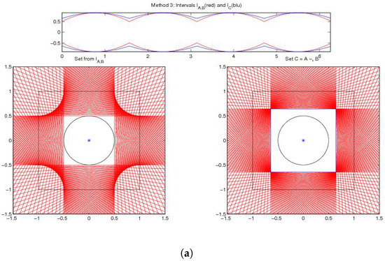
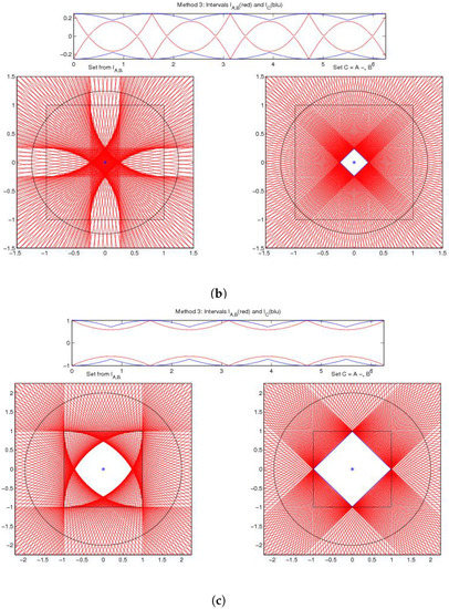
Figure 1. Example 1. $g^{*}$-difference $C^{*}=A{\ominus }_{*}{B}_{\mu }$ for (a) top: $\mu =0.5$, (b) middle: $\mu =1.25$, (c) bottom: $\mu =2.0$.

In the second case $\mu =1.25$, the $g^{*}$-difference $C^{*}=A{\ominus }_{*}{B}_{\mu }$ is pictured on the right of Figure 1b; we obtain $∥C^{*}∥=d_H(A,B)=0.25$; the geometric difference $A\stackrel{*}{-}B$ and set $D_{A,B}$ are empty, the directed difference is not proper and $A{\ominus }_{gH}{B}_{\mu }$ does not exist.

In the third case $\mu =2.0$, the $g^{*}$-difference $C^{*}=A{\ominus }_{*}{B}_{\mu }$ is pictured on the right of Figure 1c; we obtain $∥C^{*}∥=d_H(A,B)=1$; the geometric difference $A\stackrel{*}{-}B$ and the directed difference are well defined (not empty and proper, respectively) and pictured on the left of Figure 1c. Consider that $A\stackrel{*}{-}B\subset C^{*}$ and $A{\ominus }_{gH}{B}_{\mu }$ does not exist.

Example 2: This example is a modified version of the one given by Rubinov and Akhundov in [44]; $A=\{x\in {\mathbb{R}}^2|∥x∥\le 1\}$ is the unit circle and $B_{a,\mu }=[-a,a]\times [-\mu ,\mu ]$ is a rectangle with a small base $a\ge 0$. In [44] the case $a=0$ is examined; we have chosen $a=0.01$, to better visualize the construction; as in [44], the values $\mu \in \{0.5,1.0,1.75\}$ are used.

In the first case $a=0.01$ and $\mu =0.5$, the $g^{*}$-difference $C^{*}=A{\ominus }_{*}{B}_{\mu }$ is pictured on the right of Figure 2a; we obtain $∥C^{*}∥=d_H(A,B)=1-a$; the geometric difference $A\stackrel{*}{-}B$ and the directed difference are well defined (not empty and proper, respectively) and pictured on the left of Figure 2a. Consider that $A\stackrel{*}{-}B\subset C^{*}$ and $A{\ominus }_{gH}{B}_{\mu }$ does not exist.

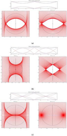
Figure 2. Example 2. $g^{*}$-difference $C^{*}=A{\ominus }_{*}{B}_{a,\mu }$ for $a=0.01$ and (a) top: $\mu =0.5$, (b) middle: $\mu =1.25$, (c) bottom: $\mu =1.0$.

In the second case $a=0.01$ and $\mu =1.75$, the $g^{*}$-difference $C^{*}=A{\ominus }_{*}{B}_{\mu }$ is pictured on the right of Figure 2b; we obtain $∥C^{*}∥=d_H(A,B)=1-a$; the geometric difference $A\stackrel{*}{-}B$ is empty, the directed difference is not proper and $A{\ominus }_{gH}{B}_{\mu }$ does not exist.

In the third case $a=0.01$ and $\mu =1.0$, the $g^{*}$-difference $C^{*}=A{\ominus }_{*}{B}_{\mu }$ is pictured on the right of Figure 2c; also here we obtain $∥C^{*}∥=d_H(A,B)=1-a$; the geometric difference is $A\stackrel{*}{-}B=0$, the directed difference is not proper and $A{\ominus }_{gH}{B}_{\mu }$ does not exist.

Example 3: This example works with polygons. Consider the two convex polygons

$$\begin{array}{ccc}\hfill A^{\prime }& =& conv\{a_1,a_2,a_3,a_4,a_5\}\hfill \\ \hfill B^{\prime }& =& conv\{b_1,b_2,b_3,b_4,b_5\}\hfill \end{array}$$

defined in terms of their vertices $a_1=(-1.5,0)$, $a_2=(0,3.5)$, $a_3=(3.5,1)$, $a_4=(1,-1.5)$, $a_5=(-1,-1.5)$ and $b_1=(-3,0)$, $b_2=(-1,2)$, $b_3=(1.5,1)$, $b_4=(1.5,0)$, $b_5=(0,-1.5)$. In the first case, we compute the difference $A{\ominus }_{*}B$ for $A=A^{\prime }$ and $B=B^{\prime }$. In the second case we use $A=A^{\prime }+B^{\prime }$ (the convex polygon obtained as the addition of the two polygons $A^{\prime }$ and $B^{\prime }$) and $B=B^{\prime }$, so that B is a summand of A and $A{\ominus }_{H}B$, the classical Hukuhara difference, exists.

For the first case with $A=A^{\prime }$ and $B=B^{\prime }$, the $g^{*}$-difference $C^{*}=A{\ominus }_{*}{B}_{\mu }$ is pictured on the right of Figure 3a; we obtain $∥C^{*}∥=d_H(A,B)=2$; the geometric difference $A\stackrel{*}{-}B$ is empty, the directed difference is not proper and $A{\ominus }_{gH}{B}_{\mu }$ does not exist.

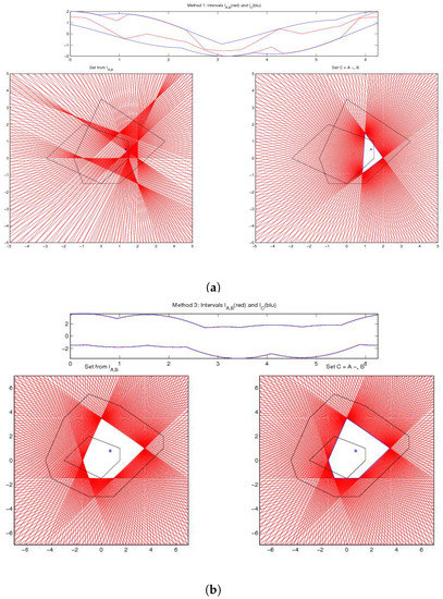
Figure 3. Example 3. $g^{*}$-difference $C^{*}=A{\ominus }_{*}{B}_{a,\mu }$ for (a) top: $A=A^{\prime },B=B^{\prime }$, (b) bottom: $A=A^{\prime }+B^{\prime },B=B^{\prime }$.

In the second case with $A=A^{\prime }+B^{\prime }$ and $B=B^{\prime }$, the $g^{*}$-difference $C^{*}=A{\ominus }_{*}{B}_{\mu }$, the geometric difference $A\stackrel{*}{-}B$ and the (proper) directed difference exist and coincide, as pictured on the left and the right sides of Figure 3b; we obtain $∥C^{*}∥=d_H(A,B)=2$.

Example 4: In our last example $A={[-1,1]}^2$ is the unit square centered at the origin and B is an “inclined” rectangle formed around one of the diagonals of A and with four vertices $b_1=(-1,-0.75)$, $b_2=(-0.75,-1)$, $b_3=(1,0.75)$, $b_4=(0.75,1)$. In this case, the geometric difference is $A\stackrel{*}{-}B=0$ (only $0+B\subset A$) and the directed difference is not proper (left of Figure 4). We obtain $∥C^{*}∥=d_H(A,B)=1.2374$ (right of Figure 4).

Figure 4. Example 4. $g^{*}$-difference $C^{*}=A{\ominus }_{*}B$.

5. Extension to Convex Fuzzy Sets

A general fuzzy set over ${\mathbb{R}}^n$ (the universe) is usually defined by its membership function $\mu :{\mathbb{R}}^n⟶[0,1]$ and a fuzzy set u of ${\mathbb{R}}^n$ is uniquely characterized by the pairs $(x,\mu (x\left)\right)$ for each $x\in {\mathbb{R}}^n$; the value $\mu \left(x\right)$ is the membership grade of x for a fuzzy set over ${\mathbb{R}}^n$ (see [45,46] or [47] for the origins of Fuzzy Set Theory).

We will denote by $u,v,w,\dots$ the fuzzy sets and the corresponding membership functions, e.g., $u\left(x\right)$, $u\left(t\right)$ will denote directly the membership grade of x, t.

The support of a fuzzy set u is the (crisp) subset of points of ${\mathbb{R}}^n$ at which the membership grade $u\left(x\right)$ is positive: $supp\left(u\right)=\left\{x\right|x\in {\mathbb{R}}^n$, $u\left(x\right)>0\}$. For $\alpha \in ]0,1],$ the $\alpha -$level cut of u (or simply the $\alpha -cut$) is defined by ${\left[u\right]}_{\alpha }=\left\{x\right|x\in {\mathbb{R}}^n,$$u\left(x\right)\ge \alpha \}$ and for $\alpha =0$ (or $\alpha \to +0$) by the closure of the support${\left[u\right]}_0=cl\left\{x\right|x\in {\mathbb{R}}^n,$$u\left(x\right)>0\}$.

A particular class of fuzzy sets u is when the support and the $\alpha -cuts$ are compact and convex set; equivalently, ${\mu }_u$ is quasi-concave and upper semi-continuous. We will also require that the membership function is normal, i.e., the core ${\left[u\right]}_1=\left\{x\right|u\left(x\right)=1\}$ is compact and non-empty. Without ambiguity, 0 will denote the origin of ${\mathbb{R}}^n$ or the crisp set $\left\{0\right\}.$

We will denote by ${\mathcal{F}}^n$ the set of the fuzzy sets with the properties above (also called fuzzy quantities). The space ${\mathcal{F}}^n$ is structured by an addition and a scalar multiplication, defined either by the level sets or, equivalently, by the Zadeh extension principle.

Let $u,v\in {\mathcal{F}}^n$ have membership functions ${\mu }_u,$${\mu }_v$ and $\alpha -cuts$${\left[u\right]}_{\alpha },$${\left[v\right]}_{\alpha },$$\alpha \in [0,1]$ respectively. In the unidimensional case $u\in \mathcal{F}$, we will denote by ${\left[u\right]}_{\alpha }=[u_{\alpha }^{-},u_{\alpha }^{+}]$ the compact intervals forming the $\alpha -cuts$ and the fuzzy quantities will be called fuzzy numbers.

The addition $u+v\in {\mathcal{F}}^n$ and the scalar multiplication $ku\in {\mathcal{F}}^n$ have level cuts

$$\begin{array}{ccc}\hfill {[u+v]}_{\alpha }& =& {\left[u\right]}_{\alpha }+{\left[v\right]}_{\alpha }=\{x+y|x\in {\left[u\right]}_{\alpha },y\in {\left[v\right]}_{\alpha }\}\hfill \end{array}$$

(57)

$$\begin{array}{ccc}\hfill {\left[ku\right]}_{\alpha }& =& k{\left[u\right]}_{\alpha }=\left\{kx\right|x\in {\left[u\right]}_{\alpha }\}.\hfill \end{array}$$

(58)

The H-difference $u{⊝}_{H}v=w$ exists if $u=v+w$ with $w\in {\mathcal{F}}^n$; the gH-difference for fuzzy numbers can be defined as follows ([12]):

Definition 17.

Given $u,v\in {\mathcal{F}}^n$, the gH-difference is the fuzzy quantity $w\in {\mathcal{F}}^n$, if it exists, such that

$$u{⊝}_{gH}v=w⟺\left\{\begin{array}{ccc}& \left(i\right)\hfill & u=v+w\hfill \\ or\hfill & \left(ii\right)\hfill & v=u+(-1)w\hfill \end{array}\right.;$$

(59)

If $u{⊝}_{gH}v$ and $u{⊝}_{H}v$ exist, $u{⊝}_{H}v=u{⊝}_{gH}v$; if (i) and (ii) are satisfied simultaneously, then w is a crisp quantity. Also, $u{⊝}_{gH}u=u{⊝}_{H}u=0$.

An equivalent definition of $w=u{⊝}_{gH}v$ can be obtained in terms of support functions in a way similar to Equation (15)

$$s_w(p;\alpha )=⟨\begin{array}{cc}{s}_u(p;\alpha )-s_v(p;\alpha )\hfill & \mathrm{in}\mathrm{case}\left(i\right)\hfill \\ s_{(-1)v}(p;\alpha )-s_{(-1)u}(p;\alpha )\hfill & \mathrm{in}\mathrm{case}\left(ii\right)\hfill \end{array},\alpha \in [0,1]$$

(60)

where for a fuzzy quantity u, the support functions are considered for each $\alpha -cut$ and defined to characterize the $\alpha -cuts$${\left[u\right]}_{\alpha }$:

$$\begin{array}{ccc}\hfill s_u& :& {\mathbb{S}}^{n-1}\times [0,1]⟶\mathbb{R}\mathrm{defined}\mathrm{by}\hfill \\ \hfill s_u(p;\alpha )& =& sup\left\{⟨p,x⟩\right|x\in {\left[u\right]}_{\alpha }\}\mathrm{for}\mathrm{each}p\in {\mathbb{S}}^{n-1},\alpha \in [0,1].\hfill \end{array}$$

The gH-difference $u{⊝}_{gH}v$ in the fuzzy context has been introduced in [12]; it is the fuzzy quantity with $\alpha -cuts$

$${\left[u{⊝}_{gH}v\right]}_{\alpha }=cl\bigcup _{\beta \ge \alpha }\left({\left[u\right]}_{\beta }{⊝}_{gH}{\left[v\right]}_{\beta }\right)$$

(61)

where the gH-differences on the right, assuming they exist for all $\alpha \in [0,1]$, are intended into ${\mathcal{K}}^n$ by Equation (59).

In general, the fuzzy set defined by the union (61) is not convex; if a convex fuzzy set is required, then the compact sets are convexified (by convex hull), obtaining the convexified gH-difference

$${\left[u{⊝}_{cgH}v\right]}_{\alpha }=cl\left(conv\bigcup _{\beta \ge \alpha }\left({\left[u\right]}_{\beta }{⊝}_{gH}{\left[v\right]}_{\beta }\right)\right).$$

(62)

The fuzzy total t-difference and the fuzzy convexified total ct-difference can be defined in a similar way, in terms of the corresponding $\alpha$-cuts, for $\alpha \in [0,1]$:

$$\begin{array}{ccc}\hfill {\left[u{⊝}_{t}v\right]}_{\alpha }& =& cl\bigcup _{\beta \ge \alpha }\left({\left[u\right]}_{\beta }{⊝}_t{\left[v\right]}_{\beta }\right),\hfill \\ \hfill {⊝}_{ct}{v]}_{\alpha }& =& cl\left(conv\bigcup _{\beta \ge \alpha }\left({\left[u\right]}_{\beta }{⊝}_{ct}{\left[v\right]}_{\beta }\right)\right).\hfill \end{array}$$

(63)

Fuzzy example 1: This example considers two convex (interacting) fuzzy sets with elliptic $\alpha$-cuts. To generate elliptic sets in ${\mathbb{R}}^2$ we use the well-known property that given a positive definite $2\times 2$ matrix Q, the set

$$E=\{x\in {\mathbb{R}}^2|⟨x,Qx⟩\le 1\}$$

(64)

is convex and elliptic (centered at the origin) and its support function is

$$s_E\left(p\right)=\sqrt{⟨p,Q^{-1}p⟩}\mathrm{for}\mathrm{all}p\in {\mathbb{S}}^1.$$

Starting with two elliptic sets U and V defined as in (64) by two positive definite matrices $Q_U$ and $Q_V$, we construct the $\alpha$-cuts of u and v

$$\begin{array}{ccc}{\left[u\right]}_{\alpha }=(1-\alpha )f_{0}U+\alpha f_{1}U& \mathrm{for}& \alpha \in [0,1]\\ {\left[v\right]}_{\alpha }=(1-\alpha )g_{0}V+\alpha g_{1}V& \mathrm{for}& \alpha \in [0,1]\end{array}$$

where $f_0>f_1>0$ and $g_0>g_1>0$ are positive factors giving the supports $f_{0}U$, $g_{0}V$ and the cores $f_{1}U$, $g_{1}V$ of u and v, respectively. The used matrices are

$$Q_U=\left[\begin{array}{cc}1& 0.5\\ 0.5& 2\end{array}\right]\mathrm{and}{Q}_V=\left[\begin{array}{cc}1& -0.25\\ -0.25& 0.5\end{array}\right]$$

and, for all $\alpha \in [0,1]$, the $\alpha$-cuts of u contain the $\alpha$-cuts of v. The ct-difference is pictured in Figure 5.

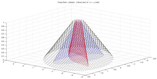
Figure 5. Fuzzy Example 1. Fuzzy sets u (black), v (blue) and fuzzy ct-difference $w^{*}=u{\ominus }_{ct}v$ (red).

Fuzzy example 2: In this example, the $\alpha$-cuts of u and v are polygons

$$\begin{array}{lll}{\left[u\right]}_{\alpha }=(1-\alpha )f_{0}U+\alpha f_{1}U& \mathrm{for}& \alpha \in [0,1]\\ {}_{\alpha }=(1-\alpha )g_{0}V+\alpha g_{1}V& \mathrm{for}& \alpha \in [0,1]\end{array}$$

where U and V are polygons with the two sets of vertices:

for U—$\left\{\right(2,0.4)$, $(1.6,2)$, $(0,2.4)$, $(-1.6,2)$, $(-2,0.4)$, $(-2,-0.4)$, $(-1.4,-1.4)$, $(-0.4,-1.8)$, $(0.4,-1.8)$, $(1.4,-1.4)$, $(2,-0.4)\}$, and

for V—$\left\{\right(1,0.4)$, $(0.6,1)$, $(0,1.4)$, $(-0.6,1)$, $(-1,0.4)$, $(-1,-0.4)$, $(0,-0.8)$, $(1,-0.4)\}$.

The corresponding fuzzy ct-difference is pictured in Figure 6.

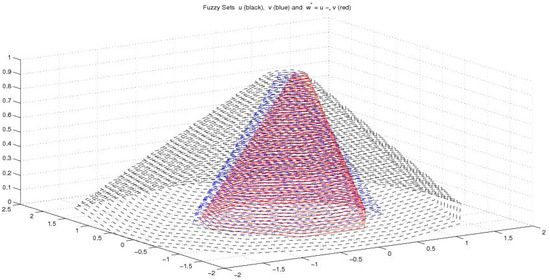
Figure 6. Fuzzy Example 2. Fuzzy sets u (black), v (blue) and fuzzy ct-difference $w^{*}=u{\ominus }_{ct}v$ (red).

6. Conclusions

In this paper we propose a general setting to define the difference sets $A\ominus B$ of multidimensional compact convex sets $A,B\subset {\mathbb{R}}^n$ (and convex fuzzy sets with bounded support) in terms of convex sets $C\subseteq A-B$ (the classical Minkowski operation) such that $A\subseteq B+C$ and $B\subseteq A-C$, which always exist. In order to overcome the possible non unicity of such sets C, we suggest to select the difference sets among the sets C above that satisfy some minimality conditions (see Section 3) that allows, additionally, to express the Pompeiu-Hausdorff distance in terms of the norm of the difference, i.e., $d_H(A,B)=∥A\ominus B∥$, using the standard norm in ${\mathbb{R}}^n$.

Application of the difference set $A\ominus B$ to the fuzzy case is obtained by the levelwise approach based on the property that the level cuts are compact convex and characterize convex fuzzy sets uniquely.

The range of possible applications of the proposed difference(s) is quite extended, following the intense research published in set-valued analysis ([48,49]), in variational analysis ([7,9,10,50]), in set-valued differential equations, among other fields, by using set difference to define differentiability.

Following the computational procedures (based on linear programming) for the difference of compact convex sets in ${\mathbb{R}}^2$, as presented in Section 4 and Section 5, additional work is in preparation for the n-dimensional case, $n>2$, in particular for special classes of convex sets, e.g., compact convex polytopes, zonoids (Minkowski sums of multidimensional segments $[a^{\left(i\right)},b^{\left(i\right)}]=$$\{(1-t)a^{\left(i\right)}+t{b}^{\left(i\right)}|t\in [0,1]\}$ with $a^{\left(i\right)},b^{\left(i\right)}\in {\mathbb{R}}^n$, $i=1,\dots ,m$) and similar. Eventually, this may allow obtaining easily computable approximations of the difference set.

References

- Markov, S. A non-standard subtraction of intervals. Serdica 1977, 3, 359–370. [Google Scholar]
- Markov, S. Extended interval arithmetic. Compt. Rend. Acad. Bulg. Sci. 1977, 30, 1239–1242. [Google Scholar]
- Markov, S. Calculus for interval functions of a real variable. Computing 1979, 22, 325–377. [Google Scholar] [CrossRef]
- Markov, S. On the Algebra of Intervals and Convex Bodies. J. Univers. Comput. Sci. 1998, 4, 34–47. [Google Scholar]
- Hukuhara, M. Integration des applications measurables dont la valeur est un compact convexe. Funkcialaj Ekvacioj 1967, 10, 205–223. [Google Scholar]
- Pontryagin, L.S. On linear differential games, II. Sov. Math. Dokl. 1967, 8, 910–912. [Google Scholar]
- Demyanov, V.F.; Rubinov, A.M. Constructive Nonsmooth Analysis; Peter Lang: Frankfurt, Germany, 1995. [Google Scholar]
- Gao, Y. Demyanov difference of two sets and optimality conditions of Lagrange multiplier type for constrained quasidifferentiable optimization. J. Optim. Theory Appl. 2000, 104, 377–394. [Google Scholar] [CrossRef]
- Mordukhovich, B.S. Variational Analysis and Generalized Differentiation I: Basic Theory; Springer: Berlin, Germany, 2006. [Google Scholar]
- Mordukhovich, B.S. Variational Analysis and Generalized Differentiation II: Applications; Springer: Berlin, Germany, 2006. [Google Scholar]
- Penot, J.-P. On the minimization of difference functions. J. Glob. Optim. 1998, 12, 373–382. [Google Scholar] [CrossRef]
- Stefanini, L. A generalization of Hukuhara-difference and division for interval and fuzzy arithmetic. Fuzzy Sets Syst. 2010, 161, 1564–1584. [Google Scholar] [CrossRef]
- Bede, B. Mathematics of Fuzzy Sets and Fuzzy Logic; Studies in Fuzziness and Soft Computing Series n. 295; Springer: Berlin/Heidelberg, Germany, 2013. [Google Scholar]
- Bede, B.; Stefanini, L. Generalized differentiability of fuzzy valued functions. Fuzzy Sets Syst. 2013, 230, 119–141. [Google Scholar] [CrossRef]
- Stefanini, L.; Bede, B. Generalized fuzzy differentiability with LU-parametric representation. Fuzzy Sets Syst. 2014, 257, 184–203. [Google Scholar] [CrossRef]
- Stefanini, L.; Arana-Jimenez, M. Karush-Kuhn-Tucker conditions for interval and fuzzy optimization in several variables under total and directional generalized differentiability. Fuzzy Sets Syst. 2019, 362, 1–34. [Google Scholar] [CrossRef]
- Baier, R.; Farkhi, E. Differences of Convex Compact Sets in the Space of Directed Sets, Part I: The Space of Directed Sets. Set-Valued Anal. 2001, 9, 217–245. [Google Scholar] [CrossRef]
- Baier, R.; Farkhi, E. Differences of Convex Compact Sets in the Space of Directed Sets, Part II: Visualization of Directed Sets. Set-Valued Anal. 2001, 9, 247–272. [Google Scholar] [CrossRef]
- Baier, R.; Farkhi, E.; Roshchina, V. The directed and Rubinov subdifferentials of quasidifferentiable functions, Part I: Definition and examples. Nonlinear Anal. 2012, 75, 1074–1088. [Google Scholar] [CrossRef]
- Baier, R.; Farkhi, E.; Roshchina, V. The directed and Rubinov subdifferentials of quasidifferentiable functions, Part II: Calculus. Nonlinear Anal. 2012, 75, 1058–1073. [Google Scholar] [CrossRef]
- Pallaschke, D.; Urbanski, R. Pairs of Compact Convex Sets, Fractional Arithmetic with Convex Sets; Kluwer Academic Publishers: Dordrecht, The Netherlands, 2002. [Google Scholar]
- Banks, H.T.; Jacobs, M.Q. A differential calculus for multifunctions. J. Math. Anal. Appl. 1970, 29, 246–272. [Google Scholar] [CrossRef]
- Radstrom, H. An embedding theorem for spaces of convex sets. Proc. Am. Math. Soc. 1952, 3, 165–169. [Google Scholar] [CrossRef]
- Bede, B.; Gal, S.G. Generalizations of the differentiability of fuzzy number valued functions with applications to fuzzy differential equations. Fuzzy Sets Syst. 2005, 151, 581–599. [Google Scholar] [CrossRef]
- Bede, B.; Stefanini, L. Solution of fuzzy differential equations with generalized differentiability using LU-parametric representation. In Proceedings of the EUSFLAT/LFA 2011 Conference, Aix-Les-Bains, France, 18-22 July 2011; Galichet, S., Montero, J., Mauris, G., Eds.; Atlantis Press: Paris, France, 2011; Volume 1, pp. 785–790. [Google Scholar]
- Buckley, J.J.; Qu, Y. Solving linear and quadratic fuzzy equations. Fuzzy Sets Syst. 1990, 38, 43–61. [Google Scholar] [CrossRef]
- Buckley, J.J.; Qu, Y. Solving fuzzy equations: A new solution concept. Fuzzy Sets Syst. 1991, 39, 291–303. [Google Scholar] [CrossRef]
- Buckley, J.J.; Qu, Y. Solving systems of linear fuzzy equations. Fuzzy Sets Syst. 1991, 43, 33–43. [Google Scholar] [CrossRef]
- Buckley, J.J. Solving fuzzy equations. Fuzzy Sets Sys. 1992, 50, 1–14. [Google Scholar] [CrossRef]
- Dubois, D.; Prade, H. Fuzzy set-theoretic differences and inclusions and their use in the analysis of fuzzy equations. Control Cybern. 1984, 13, 129–146. [Google Scholar]
- Laksmikantham, V.; Mohapatra, R.N. Theory of Fuzzy Differential Equations and Inclusions; Taylor and Francis: New York, NY, USA, 2003. [Google Scholar]
- Malinowski, M.T. Bipartite Fuzzy Stochastic Differential Equations with Global Lipschitz Condition. Math. Probl. Eng. 2016, 2016, 3830529. [Google Scholar] [CrossRef]
- Stefanini, L.; Bede, B. Generalized Hukuhara differentiability of interval valued functions and interval differential equations. Nonlinear Anal. 2009. [Google Scholar] [CrossRef]
- Stefanini, L.; Bede, B. Some Notes on Generalized Hukuhara Differentiability of Interval Valued Functions and Interval Differential Equations; EMS Working Paper Series; Faculty of Economics: Urbino, Italy, 2012; Available online: http://ideas.repec.org/f/pst233.html (accessed on 16 March 2019).
- Wang, C.; Agarwal, R.P.; O’Regan, D. Calculus of fuzzy vector-valued functions and almost periodic fuzzy vector-valued functions on time scales. Fuzzy Sets Syst. 2018. [Google Scholar] [CrossRef]
- Stefanini, L. Computational Procedures for the Difference of Compact Convex Sets; EMS Working Paper Series; Faculty of Economics: Urbino, Italy, in preparation.
- Diamond, P.; Kloeden, P. Metric Spaces of Fuzzy Sets; World Scientific: Singapore, 1994. [Google Scholar]
- Diamond, P.; Koerner, R. Extended fuzzy linear models and least squares estimates. Comput. Math. Appl. 1997, 33, 15–32. [Google Scholar] [CrossRef]
- Diamond, P.; Kloeden, P.; Rubinov, A.; Vladimirov, A. Comparative properties of three metrics in the space of compact convex sets. Set-Valued Anal. 1997, 5, 267–289. [Google Scholar] [CrossRef]
- Schneider, R. Convex Bodies: The Brunn-Minkowski Theory; Cambridge University Press: Cambridge, UK, 1993. [Google Scholar]
- Markov, S. On the algebraic properties of convex bodies and some applications. J. Convex Anal. 2000, 7, 129–166. [Google Scholar]
- Stefanini, L. On the generalized LU-fuzzy derivative and fuzzy differential equations. In Proceedings of the FUZZIEEE 2007 Conference, London, UK, 23–26 July 2007; Available online: http://ideas.repec.org/f/pst233.html (accessed on 16 March 2019). [CrossRef]
- Martinez-Legaz, J.-E.; Penot, J.-P. Regularization by erasement. Math. Scand. 2006, 98, 97–124. [Google Scholar] [CrossRef][Green Version]
- Rubinov, A.M.; Akhundov, I.S. Difference of compact sets in the sense of Demyanov and its application to nonsmooth analysis. Optimization 1992, 23, 179–188. [Google Scholar] [CrossRef]
- Zadeh, L.A. Fuzzy sets. Inf. Control 1965, 8, 338–353. [Google Scholar] [CrossRef]
- Zadeh, L.A. Concept of a linguistic variable and its application to approximate reasoning, I. Inf. Sci. 1975, 8, 199–249. [Google Scholar] [CrossRef]
- Zadeh, L.A. Fuzzy sets as a basis for a theory of possibility. Fuzzy Sets Syst. 1978, 1, 3–28. [Google Scholar] [CrossRef]
- Aubin, J.P.; Frankowska, H. Set-Valued Analysis; Birkhauser-Verlag: Boston, MA, USA, 1990. [Google Scholar]
- Rockafellar, R.T. Convex Analysis; Princeton Univ. Press: Princeton, NJ, USA, 1970. [Google Scholar]
- Rockafellar, R.T.; Wets, R.J.-B. Variational Analysis; Springer: Berlin, Germany, 1998. [Google Scholar]
© 2019 by the authors. Licensee MDPI, Basel, Switzerland. This article is an open access article distributed under the terms and conditions of the Creative Commons Attribution (CC BY) license (http://creativecommons.org/licenses/by/4.0/).