Shifting Operators in Geometric Quantization

Abstract

The original Bohr-Sommerfeld theory of quantization did not give operators of transitions between quantum quantum states. This paper derives these operators, using the first principles of geometric quantization.

1. Introduction

Even though the Bohr–Sommerfeld theory was very successful in predicting some physical results, it was never accepted by physicists as a valid quantum theory in the same class as the Schrödinger theory or the Bargmann–Fock theory. The reason for this was that the original Bohr–Sommerfeld theory did not provide operators of transition between quantum states. The need for such operators in the Bohr–Sommerfeld quantization was already pointed out by Heisenberg [1]. The aim of this paper is to derive operators of transition between quantum states in the Bohr–Sommerfeld theory, which we call shifting operators, from the first principles of geometric quantization.

The first step of geometric quantization of a symplectic manifold $(P,\omega )$ is called prequantization. It consists of the construction of a complex line bundle $\pi :L\to P$ with connection whose curvature form satisfies a prequantization condition relating it to the symplectic form $\omega$. A comprehensive study of prequantization, from the point of view of representation theory, was given by Kostant in [2]. The work of Souriau [3] was aimed at quantization of physical systems, and studied a circle bundle over phase space. In Souriau’s work, the prequantization condition explicitly involved Planck’s constant $\mathrm{h}$. In [4], Blattner combined the approaches of Kostant and Souriau by using the complex line bundle with the prequantization condition involving Planck’s constant. Since then, geometric quantization has been an effective tool in quantum theory.

We find it convenient to deal with connection and curvature of complex line bundles using the theory of principal and associated bundles [5]. In this framework, the prequantization condition reads

$$\mathrm{d}\beta ={\left({\pi }^{\times }\right)}^{*}(-\frac{1}{\mathrm{h}}\omega ),$$

where $\beta$ is the connection 1-form on the principal ${\mathbb{C}}^{\times }$-bundle ${\pi }^{\times }:L^{\times }\to P$ associated to the complex line bundle $\pi :L\to P$, and ${\mathbb{C}}^{\times }$ is the multiplicative group of nonzero complex numbers.

The aim of prequantization is to construct a representation of the Poisson algebra $(C^{\infty }\left(P\right),\{,\},·)$ of $(P,\omega )$ on the space of sections of the line bundle L. Each Hamiltonian vector field $X_f$ on P lifts to a unique ${\mathbb{C}}^{\times }$-invariant vector field $Z_f$ on $L^{\times }$ that preserves the principal connection $\beta$ on $L^{\times }$. If the vector field $X_f$ is complete, then it generates a 1-parameter group ${\mathrm{e}}^{t{X}_f}$ of symplectomorphisms of $(P,\omega )$. Then, the vector field $Z_f$ is complete and it generates a 1-parameter group ${\mathrm{e}}^{t{Z}_f}$ of connection preserving diffeomorphisms of the bundle $(L^{\times },\beta )$, called quantomorphisms, which cover the 1-parameter group ${\mathrm{e}}^{t{X}_f}$. The term quantomorphism was introduced by Souriau [3] in the context of $\mathrm{SU}\left(n\right)$-principal bundles and discussed in detail in his book [6]. The construction discussed here follows [7], where the term quantomorphism was not used. In this case, ${\mathrm{e}}^{t{X}_f}$ and ${\mathrm{e}}^{t{Z}_f}$ are 1-parameter groups of diffeomorphisms of P and $L^{\times }$, respectively. We refer to ${\mathrm{e}}^{t{X}_f}$ and ${\mathrm{e}}^{t{Z}_f}$ as flows of $X_f$ and $Z_f$. Since L is an associated bundle of $L^{\times }$, the action ${\mathrm{e}}^{t{Z}_f}:L^{\times }\to L^{\times }$, induces an action ${\widehat{\mathrm{e}}}^{t{Z}_f}:L\to L,$ which gives rise to an action on smooth sections $\sigma$ of L by push forwards, $\sigma \mapsto {\widehat{\mathrm{e}}}_{*}^{t{Z}_f}\sigma ={\widehat{\mathrm{e}}}^{t{Z}_f}\circ \sigma \circ {\mathrm{e}}^{-t{X}_f.}$. Although ${\widehat{\mathrm{e}}}_{*}^{t{Z}_f}\sigma$ may not be defined for all sections $\sigma$ and all t, its derivative at $t=0$ is defined for all smooth sections. The prequantization operator

$${\mathcal{P}}_f\sigma =i\mathsf{ћ}{\displaystyle \frac{\mathrm{d}}{\mathrm{d}t}}{|}_{t=0}{\widehat{\mathrm{e}}}_{*}^{t{Z}_f}\sigma ,$$

(1)

where $\mathsf{ћ}$ is Planck’s constant $\mathrm{h}$ divided by $2\pi$, is a symmetric operator on the Hilbert space $\mathsf{𝕳}$ of square integrable sections of L. The operator ${\mathcal{P}}_f$ is self adjoint if $X_f$ is complete.

The whole analysis of prequantization is concerned with global Hamiltonian vector fields. Since every vector field on $(P,\omega )$ that preserves the symplectic form is locally Hamiltonian, it is of interest to understand how much of prequantization can be extended to this case. In particular, we are interested in the case where the locally Hamiltonian vector field is the vector field $X_{\vartheta }$ of the integer angle variable $\vartheta$ that is defined up to an additive term $n,$ where $n\in \mathbb{Z}.$ For a globally Hamiltonian vector field $X_f$,

$${\widehat{\mathrm{e}}}_{*}^{t{Z}_f}\sigma ={\mathrm{e}}^{-2\pi itf/\mathrm{h}}{\widehat{\mathrm{e}}}_{*}^{t\mathrm{lift}{X}_f}\sigma ,$$

(2)

where ${\widehat{\mathrm{e}}}_{*}^{t\mathrm{lift}{X}_f}\sigma$ is the horizontal transport of section $\sigma$ by parameter t along integral curves of $X_f.$Replacing f by a multivalued function $\vartheta$, defined up to an additive n, yields the multivalued expression

$${\widehat{\mathrm{e}}}_{*}^{t{Z}_{\vartheta }}\sigma ={\mathrm{e}}^{-it\vartheta /\mathrm{h}}{\widehat{\mathrm{e}}}_{*}^{t\mathrm{lift}{X}_{\vartheta }}\sigma .$$

(3)

We observe that, for $t=\mathrm{h}$, Equation (3) gives a single valued expression

$${\widehat{\mathrm{e}}}_{*}^{\mathrm{h}{Z}_{\vartheta }}\sigma ={\mathrm{e}}^{-i\vartheta }{\widehat{\mathrm{e}}}_{*}^{\mathrm{h}\mathrm{lift}{X}_{\vartheta }}\sigma .$$

(4)

The shifting operator

$${\mathit{a}}_{X_{\vartheta }}={\widehat{\mathrm{e}}}_{*}^{\mathrm{h}{Z}_{\vartheta }}={\mathrm{e}}^{-i\vartheta }{\widehat{\mathrm{e}}}_{*}^{\mathrm{h}\mathrm{lift}{X}_{\vartheta }}$$

(5)

is an operator on $\mathfrak{H},$ which shifts the support of $\sigma \in \mathfrak{H}$ by $\mathrm{h}$ along the integral curve of $X_{\vartheta }$. If the vector field $X_{\vartheta }$ is complete, then ${\mathit{a}}_{X_{\vartheta }}^n={\widehat{\mathrm{e}}}_{*}^{n\mathrm{h}{Z}_{\vartheta }}$ for every $n\in \mathbb{Z}$.

Our results provide an answer to Heisenberg’s criticism that in Bohr–Sommerfeld theory there are not enough operators to describe transitions between quantum states [1].

Superficially, the shifting operator ${\mathit{a}}_{X_{\theta }}={{\mathrm{e}}^{i\theta }{\widehat{\mathrm{e}}}^{ћ\mathrm{lift}{X}_{\theta }}}_{*}$, see Equation (5), appears to be a quantization of an angle $\theta =2\pi \vartheta$. It depends on $\theta$ and has the factor ${\mathrm{e}}^{-i\theta }$ considered by Dirac [8]. However, the factor ${\widehat{\mathrm{e}}}_{*}^{ћ\mathrm{lift}{X}_{\theta }}$, describing the parallel translation by $\mathsf{ћ}$ along integral curves of $X_{\theta },$ makes it nonlocal in the phase space. Therefore, ${\mathit{a}}_{X_{\theta }}$ cannot satisfy local commutation relations with any local quantum variable that is described by a differential operator. Hence, it cannot be the canonical conjugate of the corresponding action operator, or any other operator, which is local in the phase space.

In our earlier papers [9,10,11,12], we followed an algebraic analysis, similar to that used by Dirac [8], supplemented by heuristic guesses about the behaviour of the shifting operators at the points of singularity of the polarization. In particular, we assumed that ${\mathit{a}}_{X_{\vartheta }}$ vanishes on the states concentrated on a set of limit points of ${\mathrm{e}}^{t{X}_{\vartheta }}\left(p\right)$ as $t\to \infty .$ In the present paper, we derive shifting operators in the framework of geometric quantization, and extend our result to cases with a variable rank polarization.

The second stage in geometric quantization consists of the choice of a polarization, which is an involutive complex Lagrangian distribution F on the phase space. Suppose that P is the cotangent bundle space of the configuration space. In this case, the choice of F containing the vertical directions, leads the quantum mechanics of Schrödinger. If F leads to complex analytic structure on P, we have the Bargmann–Fock theory. If F is spanned by the Hamiltonian vector fields of a completely integrable system, we have Bohr–Sommerfeld theory. Each of these theories have specific structure, which is helpful in formulation and solving problems. In the following, we restrict our investigation to the Bohr–Sommerfeld theory in order to emphasize its membership in the class of quantum theories corresponding to different polarization.

A common problem in arising in quantum theories is occurrence of singularities. Usually, one studies the geometric structure of the theory in the language of differential geometry of smooth manifolds, and then investigates the structure of singularities separately. The theory of differential spaces, introduced by Sikorski [13,14], is a powerful tool in the study of the geometry of spaces with singularities [15]. The main singularity encountered here corresponds to the fact that the polarization F spanned by the Hamiltonian vector fields of a completely integrable system does not have constant rank. This singularity is so well known that we do not have to use the language of differential spaces to get results. It should be noted that the results in [9,11] rely on the theory of differential spaces.

In conclusion, it should be mentioned that the scientists, who used visual presentation of the Bohr–Sommerfeld spectra in terms of dots on the space of the action variables, are familiar with handling shifting operators. The line segments joining two dots corresponding to quantum states represent the shifting operators between these states.

To make the paper more accessible to the reader, we have provided an introductory section with a comprehensive review of geometric quantization. Experts may omit this section and proceed directly to the next section on Bohr–Sommerfeld theory.

2. Elements of Geometric Quantization

Let $(P,\omega )$ be a symplectic manifold. Geometric quantization can be divided into three steps: prequantization, polarization, and unitarization.

2.1. Principal Line Bundles with a Connection

We begin with a brief review of connections on complex line bundles.

Let ${\mathbb{C}}^{\times }$ denote the multiplicative group of nonzero complex numbers. Its Lie algebra ${\mathfrak{c}}^{\times }$ is isomorphic to the abelian Lie algebra $\mathbb{C}$ of complex numbers. Different choices of the isomorphism $\iota :\mathbb{C}\to {\mathfrak{c}}^{\times }$ lead to different factors in various expressions. Here, to each $c\in \mathbb{C}$ we associate the 1-parameter subgroup $t\mapsto {\mathrm{e}}^{2\pi itc}$ of ${\mathbb{C}}^{\times }$. In other words, we take

$$\iota :\mathbb{C}\to {\mathfrak{c}}^{\times }:c\mapsto \iota \left(c\right)=2\pi ic.$$

(6)

The prequantization structure for $(P,\omega )$ consists of a principal ${\mathbb{C}}^{\times }$ bundle ${\pi }^{\times }:L^{\times }\to P$ and a ${\mathfrak{c}}^{\times }$-valued ${\mathbb{C}}^{\times }$-invariant connection 1-form $\beta$ satisfying

$$\mathrm{d}\beta ={\left({\pi }^{\times }\right)}^{*}(-\frac{1}{\mathrm{h}}\omega ),$$

(7)

where h is Planck’s constant. The prequantization condition requires that the cohomology class $[-\frac{1}{\mathrm{h}}\omega ]$ is integral, that is, it lies in ${\mathrm{H}}^2(P,\mathbb{Z})$, otherwise the ${\mathbb{C}}^{\times }$ principal bundle ${\pi }^{\times }:L^{\times }\to P$ would not exist.

Let $Y_c$ be the vector field on $L^{\times }$ generating the action of ${\mathrm{e}}^{2\pi itc}$ on $L^{\times }$. In other words, the 1-parameter group ${\mathrm{e}}^{t{Y}_c}$ of diffeomorphisms of $L^{\times }$ generated by $Y_c$ is

$${\mathrm{e}}^{t{Y}_c}:L^{\times }\to L^{\times }:{\ell }^{\times }\to {\ell }^{\times }{\mathrm{e}}^{2\pi itc}.$$

(8)

The connection 1-form $\beta$ is normalized by the requirement

$$⟨\beta |Y_c⟩=c.$$

(9)

For each $c\ne 0$, the vector field, $Y_c$ spans the vertical distribution $\mathrm{ver}T{L}^{\times }$ tangent to the fibers of ${\pi }^{\times }:L^{\times }\to P$. The horizontal distribution $\mathrm{hor}T{L}^{\times }$ on $L^{\times }$ is the kernel of the connection 1-form $\beta$, that is,

$$\mathrm{hor}T{L}^{\times }=ker\beta .$$

(10)

The vertical and horizontal distributions of $L^{\times }$ give rise to the direct sum $T{L}^{\times }=\mathrm{ver}T{L}^{\times }\oplus \mathrm{hor}T{L}^{\times }$, which is used to decompose any vector field Z on $L^{\times }$ into its vertical and horizontal components, $Z=\mathrm{ver}Z+\mathrm{hor}Z$. Here, the vertical component $\mathrm{ver}Z$ has range in $\mathrm{ver}T{L}^{\times }$ and the horizontal component has range in $\mathrm{hor}T{L}^{\times }$.

If X is a vector field on P, the unique horizontal vector field on $L^{\times }$, which is ${\pi }^{\times }$-related to X, is called the horizontal lift of X and is denoted by $\mathrm{lift}X$. In other words, $\mathrm{lift}X$ has range in the horizontal distribution $\mathrm{hor}T{L}^{\times }$ and satisfies

$$T{\pi }^{\times }\circ \mathrm{lift}X=X\circ {\pi }^{\times }.$$

(11)

Claim 1.

A vector field Z on $L^{\times }$ is invariant under the action of ${\mathbb{C}}^{\times }$ on $L^{\times }$ if and only if the horizontal component of Z is the horizontal lift of its projection X to P, that is, $\mathrm{hor}Z=\mathrm{lift}X$ and there is a smooth function $\kappa :P\to \mathbb{C}$ such that $\mathrm{ver}Z=Y_{\kappa \left(p\right)}$ on $L_p^{\times }={\left({\pi }^{\times }\right)}^{-1}\left(p\right)$.

Proof. 

Since the direct sum $T{L}^{\times }=\mathrm{ver}T{L}^{\times }\oplus \mathrm{hor}T{L}^{\times }$ is invariant under the ${\mathbb{C}}^{\times }$ action on $L^{\times }$, it follows that the vector field Z is invariant under the action of ${\mathbb{C}}^{\times }$ if and only if $\mathrm{hor}Z$ and $\mathrm{ver}Z$ are ${\mathbb{C}}^{\times }$-invariant. However, $\mathrm{hor}Z$ is ${\mathbb{C}}^{\times }$ invariant if $T{\pi }^{\times }\circ \mathrm{hor}Z=X\circ {\pi }^{\times }$ for some vector field X on P, that is, $\mathrm{hor}Z=\mathrm{lift}X$. However, this holds by definition. On the other hand, the vertical distribution $\mathrm{ver}T{L}^{\times }$ is spanned by the vector fields $Y_c$ for $c\in \mathbb{C}$. Hence, $\mathrm{ver}Z$ is ${\mathbb{C}}^{\times }$-invariant if and only if for every fiber $L_p^{\times }$ the restriction of $\mathrm{ver}Z$ to $L_p^{\times }$ coincides with the restriction of $Y_c$ to $L_p^{\times }$ for some $c\in \mathbb{C}$, that is, there is a smooth complex valued function $\kappa$ on P such that $c=\kappa \left(p\right)$. □

Let U be an open subset of P. A local smooth section $\tau :U\subseteq P\to L^{\times }$ of the bundle ${\pi }^{\times }:L^{\times }\to P$ gives rise to a diffeomorphism

$${\eta }_{\tau }:L_{|U}^{\times }=\bigcup _{p\in U}\left({\left({\pi }^{\times }\right)}^{-1}\left(p\right)\right)\to U\times {\mathbb{C}}^{\times }:{\ell }^{\times }\mapsto ({\pi }^{\times }\left({\ell }^{\times }\right),b)=(p,b),$$

where $b\in {\mathbb{C}}^{\times }$ is the unique complex number such that ${\ell }^{\times }=\tau \left(p\right)b$. In the general theory of principal bundles the structure group of the principal bundle acts on the right. In the theory of ${\mathbb{C}}^{\times }$ principal bundles, elements of $L^{\times }$ are considered to be one-dimensional frames, which are usually written on the right, see [2]. The diffeomorphism ${\eta }_{\tau }$ is called a trivialization of $L_{\mid U}^{\times }$. It intertwines the action of ${\mathbb{C}}^{\times }$ on the principal bundle $L^{\times }$ with the right action of ${\mathbb{C}}^{\times }$ on $U\times {\mathbb{C}}^{\times }$, given by multiplication in ${\mathbb{C}}^{\times }$. If a local section $\sigma :U\to L$ of $\pi :L\to P$ is nowhere zero, then it determines a trivialization ${\eta }_{\tau }:L_{\mid U}^{\times }\to U\times {\mathbb{C}}^{\times }$. Conversely, a local smooth section $\tau$ such that ${\eta }_{\tau }$ is a trivialization of $L^{\times }$ may be considered as a local nowhere zero section of L.

In particular, for every $c\in \mathbb{C}$, which is identified with the Lie algebra ${\mathfrak{c}}^{\times }$ of ${\mathbb{C}}^{\times }$, Equation (7) gives ${\mathrm{e}}^{t{Y}_c}\circ \tau ={\mathrm{e}}^{2\pi itc}\tau$. Differentiating with respect to t and then setting $t=0$ gives

$$Y_c\circ \tau =2\pi ic\tau .$$

(12)

For every smooth complex valued function $\kappa :P\to \mathbb{C}$, consider the vertical vector field $Y_{\kappa }$ such that $Y_{\kappa }\left({\ell }^{\times }\right)=Y_{\kappa \left({\pi }^{\times }\left({\ell }^{\times }\right)\right)}$ for every ${\ell }^{\times }\in L^{\times }$. The vector field $Y_{\kappa }$ is complete and the 1-parameter group of diffeomorphisms it generates is

$${\mathrm{e}}^{t{Y}_{\kappa }}:L^{\times }\to L^{\times }:{\ell }^{\times }\mapsto {\ell }^{\times }{\mathrm{e}}^{2\pi it\kappa \left({\pi }^{\times }\left({\ell }^{\times }\right)\right)}.$$

For every smooth section $\tau$ of the bundle ${\pi }^{\times }$, we have ${\mathrm{e}}^{t{Y}_{\kappa }}\circ \tau ={\mathrm{e}}^{2\pi it\kappa }\tau$ so that

$$Y_{\kappa }\circ \tau =2\pi i\kappa \tau .$$

(13)

Let X be a vector field on P and let $\mathrm{lift}X$ be its horizontal lift to $L^{\times }$. The local 1-parameter group ${\mathrm{e}}^{t\mathrm{lift}X}$ of local diffeomorphisms of $L^{\times }$ generated by $\mathrm{lift}X$ commutes with the action of ${\mathbb{C}}^{\times }$ on $L^{\times }$. For every ${\ell }^{\times }$, ${\mathrm{e}}^{t\mathrm{lift}X}\left({\ell }^{\times }\right)$ is called parallel transport of ${\ell }^{\times }$ along the integral curve of X starting at $p={\pi }^{\times }\left({\ell }^{\times }\right)$. For every $p\in P$ the map ${\mathrm{e}}^{t\mathrm{lift}X}$ sends the fiber $L_p^{\times }$ to the fiber $L_{{\mathrm{e}}^{tX}\left(p\right)}$.

There are several equivalent definitions of covariant derivative of a smooth section of the bundle ${\pi }^{\times }$ in the direction of a vector field X on P. We use the following one. The covariant derivative of the smooth section $\tau$ of the bundle ${\pi }^{\times }:L^{\times }\to P$ in the direction X is

$${\nabla }_X\tau ={\displaystyle \frac{\mathrm{d}}{\mathrm{d}t}}{|}_{t=0}{\left({\mathrm{e}}^{t\mathrm{lift}X}\right)}^{*}\tau .$$

(14)

Claim 2.

The covariant derivative of a smooth local section of the bundle ${\pi }^{\times }:L^{\times }\to P$ in the direction X is given by

$${\nabla }_X\tau =2\pi i⟨{\tau }^{*}\beta |X⟩\tau .$$

(15)

Proof. 

For every $p\in P$, we have

$$\begin{array}{cc}\hfill {\nabla }_X\tau \left(p\right)& ={\displaystyle \frac{\mathrm{d}}{\mathrm{d}t}}{|}_{t=0}{\left({\mathrm{e}}^{t\mathrm{lift}X}\right)}^{*}\tau \left(p\right)={\displaystyle \frac{\mathrm{d}}{\mathrm{d}t}}{|}_{t=0}\left({\mathrm{e}}^{-t\mathrm{lift}X}\circ \tau \circ {\mathrm{e}}^{tX}\right)\left(p\right)\hfill \\ \hfill & =-\mathrm{lift}X\left(\tau \right(p\left)\right)+T\tau \left(X\right(p\left)\right)\hfill \\ \hfill & =-\mathrm{lift}X\left(\tau \right(p\left)\right)+\mathrm{hor}\left(T\tau \right)X\left(p\right)+\mathrm{ver}\left(T\tau \right)X\left(p\right)\hfill \\ \hfill & =\mathrm{ver}\left(T\tau \right)X\left(p\right).\hfill \end{array}$$

The definition of the connection 1-form $\beta$ and Equation (13) yield

$$\mathrm{ver}(T\tau \left(X\left(p\right)\right)=Y_{⟨\beta |T\tau \circ X⟩}\left(\tau \left(p\right)\right)=2\pi i⟨\beta |T\tau \circ X⟩\tau \left(p\right).$$

Hence,

$${\nabla }_X\tau =2\pi i⟨\beta |T\tau \circ X⟩\tau ,$$

(16)

which is equivalent to Equation (15). □

2.2. Associated Line Bundles

The complex line bundle $\pi :L\to P$ associated to the ${\mathbb{C}}^{\times }$ principal bundle ${\pi }^{\times }:L^{\times }\to P$ is defined in terms of the action of ${\mathbb{C}}^{\times }$ on $(L^{\times }\times \mathbb{C})$ given by

$$\Phi :{\mathbb{C}}^{\times }\times (L^{\times }\times \mathbb{C})\to L^{\times }\times \mathbb{C}:\left(b,({\ell }^{\times },c)\right)\mapsto ({\ell }^{\times }b,b^{-1}c).$$

(17)

Since the action $\Phi$ is free and proper, its orbit space $L=(L^{\times }\times \mathbb{C})/{\mathbb{C}}^{\times }$ is a smooth manifold. A point $\ell \in L$ is the ${\mathbb{C}}^{\times }$ orbit $\left[({\ell }^{\times },c)\right]$ through $({\ell }^{\times },c)\in (L^{\times }\times \mathbb{C})$, namely,

$$\ell =\left[({\ell }^{\times },c)\right]=\{({\ell }^{\times }b,b^{-1}c)\in L^{\times }\times \mathbb{C}|b\in {\mathbb{C}}^{\times }\}.$$

(18)

The left action of ${\mathbb{C}}^{\times }$ on $\mathbb{C}$ gives rise to the left action

$$\widehat{\Phi }:{\mathbb{C}}^{\times }\times L\to L:\left(a,\left[({\ell }^{\times },c)\right]\right)\mapsto \left[({\ell }^{\times },ac)\right],$$

(19)

which is well defined because $\left[({\ell }^{\times },ac)\right]=\left[({\ell }^{\times }b,b^{-1}\left(ac\right))\right]=\left[({\ell }^{\times }b,a\left(b^{-1}c\right))\right]$ for every ${\ell }^{\times }\in L^{\times }$, every a, $b\in {\mathbb{C}}^{\times }$ and every $c\in \mathbb{C}$. The projection map ${\pi }^{\times }:L^{\times }\to P$ induces the projection map

$$\pi :L\to L/{\mathbb{C}}^{\times }=P:\ell =\left[({\ell }^{\times },c)\right]\mapsto \pi \left(\ell \right)=\pi \left(\left[({\ell }^{\times },c)\right]\right)={\pi }^{\times }\left({\ell }^{\times }\right).$$

Claim 3.

A local smooth section $\sigma :U\to L$ of the complex line bundle $\pi :L\to P$ corresponds to a unique mapping ${\sigma }^{♯}:L_{\mid U}^{\times }\to \mathbb{C}$ such that for every $p\in U$ and every ${\ell }^{\times }\in L_p^{\times }$

$$\sigma \left(p\right)=\left[({\ell }^{\times },{\sigma }^{♯}\left({\ell }^{\times }\right))\right],$$

(20)

which is ${\mathbb{C}}^{\times }$-equivariant, that is, ${\sigma }^{♯}\left({\ell }^{\times }b\right)=b^{-1}{\sigma }^{♯}\left({\ell }^{\times }\right)$.

Proof. 

Given $p\in U$ there exists $({\ell }^{\times },c)\in L^{\times }\times \mathbb{C}$ such that $\sigma \left(p\right)=\left[({\ell }^{\times },c)\right]$. Since the action of ${\mathbb{C}}^{\times }$ on $L_p^{\times }$ is free and transitive, it follows that the ${\mathbb{C}}^{\times }$ orbit $\{({\ell }^{\times }b,b^{-1}c)\in L_p^{\times }\times \mathbb{C}|b\in {\mathbb{C}}^{\times }\}$ is the graph of a smooth function from $L_p^{\times }$ to $\mathbb{C}$, which we denote by ${\sigma }_p^{♯}$. In particular, $c={\sigma }_p^{♯}\left({\ell }^{\times }\right)$ so that $\sigma \left(p\right)=\left[({\ell }^{\times },c)\right]=\left[({\ell }^{\times },{\sigma }_p^{♯}\left({\ell }^{\times }\right))\right]$. As p varies over U we get a map

$${\sigma }^{♯}:L_{\mid U}^{\times }\to \mathbb{C}:{\ell }^{\times }\mapsto {\sigma }^{♯}\left({\ell }^{\times }\right)={\sigma }_{{\pi }^{\times }\left({\ell }^{\times }\right)}^{♯}\left({\ell }^{\times }\right),$$

which satisfies Equation (20). For every $b\in {\mathbb{C}}^{\times }$, Equations (18) and (20) imply that

$$\sigma \left(p\right)=\left[({\ell }^{\times },{\sigma }^{♯}\left({\ell }^{\times }\right))\right]=\left[({\ell }^{\times }b,b^{-1}{\sigma }^{♯}\left({\ell }^{\times }\right))\right]=\left[({\ell }^{\times }b,{\sigma }^{♯}\left({\ell }^{\times }b\right))\right].$$

Hence, ${\sigma }^{♯}\left({\ell }^{\times }b\right)=b^{-1}{\sigma }^{♯}\left({\ell }^{\times }\right)$. Thus, the function ${\sigma }^{♯}$ is ${\mathbb{C}}^{\times }$-equivariant. □

If $\tau :U\to L^{\times }$ is a local smooth section of the bundle ${\pi }^{\times }:L^{\times }\to P$, then for every $p\in P$ we have $\sigma \left(p\right)=\left[(\tau \left(p\right),{\sigma }^{♯}\left(\tau \left(p\right)\right))\right]$ or $\sigma =\left[(\tau ,{\sigma }^{♯}\circ \tau )\right]$ suppressing the argument p. The function $\psi ={\sigma }^{♯}\circ \tau :U\to \mathbb{C}$ is the coordinate representation of the section $\tau$ in terms of the trivialization ${\eta }_{\tau }:L_{\mid U}^{\times }\to U\times \mathbb{C}$.

Let Z be a ${\mathbb{C}}^{\times }$-invariant vector field on $L^{\times }$. Then, Z is ${\pi }^{\times }$-related to a vector field X on P, that is, $T{\pi }^{\times }\circ Z=X\circ {\pi }^{\times }$. We denote by ${\mathrm{e}}^{tX}$ and ${\mathrm{e}}^{tZ}$ the local 1-parameter groups of local diffeomorphisms of P and $L^{\times }$ generated by X and Z, respectively. Because the vector fields X and Z are ${\pi }^{\times }$-related, we obtain ${\pi }^{\times }\circ {\mathrm{e}}^{tZ}={\mathrm{e}}^{tX}\circ {\pi }^{\times }$. In other words, the flow ${\mathrm{e}}^{tZ}$ of Z covers the flow ${\mathrm{e}}^{tX}$ of X. The local group ${\mathrm{e}}^{tZ}$ of automorphisms of the principal bundle $L^{\times }$ act on the associated line bundle L by

$${\widehat{\mathrm{e}}}^{tZ}:L\to L:\ell =\left[({\ell }^{\times },c)\right]\mapsto \left[({\mathrm{e}}^{tZ}\left({\ell }^{\times }\right),c)\right],$$

(21)

which holds for all $\ell =\left[({\ell }^{\times },c)\right]$ for which ${\mathrm{e}}^{tZ}\left({\ell }^{\times }\right)$ is defined.

Lemma 1.

The map ${\widehat{\mathrm{e}}}^{tZ}$ is a local 1-parameter group of local automorphisms of the line bundle L, which covers the local 1-parameter group ${\mathrm{e}}^{tX}$ of the vector field X on P.

Proof. 

We compute. For $\ell =\left[({\ell }^{\times },c)\right]\in L$ we have

$$\begin{array}{cc}\hfill {\widehat{\mathrm{e}}}^{(t+s)Z}\left(\ell \right)& ={\widehat{\mathrm{e}}}^{(t+s)Z}\left(\left[({\ell }^{\times },c)\right]\right)=\left[({\mathrm{e}}^{(t+s)Z}\left({\ell }^{\times }\right),c)\right]=\left[({\mathrm{e}}^{tZ}\left({\mathrm{e}}^{sZ}\left({\ell }^{\times }\right)\right),c)\right]\hfill \\ \hfill & ={\widehat{\mathrm{e}}}^{tZ}\left(\right[\left({\mathrm{e}}^{sZ}({\ell }^{\times },c)\right]={\widehat{\mathrm{e}}}^{tZ}\circ {\widehat{\mathrm{e}}}^{sZ}\left(\left[({\ell }^{\times },c)\right]\right)={\widehat{\mathrm{e}}}^{tZ}\circ {\widehat{\mathrm{e}}}^{sZ}\left(\ell \right).\hfill \end{array}$$

Hence, ${\widehat{\mathrm{e}}}^{tZ}$ is a local 1-parameter group of local diffeomorphisms. Moreover,

$$\pi \circ {\widehat{\mathrm{e}}}^{tZ}\left(\ell \right)=\pi \left(\left[({\mathrm{e}}^{tZ}\left({\ell }^{\times }\right),c)\right]\right)={\pi }^{\times }\left({\mathrm{e}}^{tZ}\left({\ell }^{\times }\right)\right)={\mathrm{e}}^{tX}\left({\pi }^{\times }\left({\ell }^{\times }\right)\right);$$

while

$${\mathrm{e}}^{tX}\circ \pi \left(\ell \right)={\mathrm{e}}^{tX}\left(\pi \left(\left[({\ell }^{\times },c)\right]\right)\right)={\mathrm{e}}^{tX}\left({\pi }^{\times }\left({\ell }^{\times }\right)\right).$$

This shows that ${\mathrm{e}}^{tZ}$ covers ${\mathrm{e}}^{tX}$. Finally, for every $\ell =\left[({\ell }^{\times },c)\right]\in L$ and every $b\in {\mathbb{C}}^{\times }$

$${\widehat{\Phi }}_b\left({\widehat{\mathrm{e}}}^{tZ}\left(\ell \right)\right)={\widehat{\Phi }}_b\left(\left[({\mathrm{e}}^{tZ}\left({\ell }^{\times }\right),c)\right]\right)=\left[({\Phi }_b\left({\mathrm{e}}^{tZ}\left({\ell }^{\times }\right)\right),c)\right]=\left[({\mathrm{e}}^{tZ}\left({\Phi }_b\left({\ell }^{\times }\right)\right),c)\right],$$

since Z is a ${\mathbb{C}}^{\times }$-invariant vector field on $L^{\times }$. Therefore,

$${\widehat{\Phi }}_b\left({\widehat{\mathrm{e}}}^{tZ}\left(\ell \right)\right)={\widehat{\mathrm{e}}}^{tZ}\left(\left[({\Phi }_b\left({\ell }^{\times }\right),c)\right]\right)={\widehat{\mathrm{e}}}^{tZ}\circ {\widehat{\Phi }}_b\left(\left[({\ell }^{\times },c)\right]\right)={\widehat{\mathrm{e}}}^{tZ}\circ {\widehat{\Phi }}_b\left(\ell \right).$$

This shows that ${\widehat{\mathrm{e}}}^{tZ}$ is a local group of automorphisms of the line bundle $\pi :L\to P$. □

If $Z=\mathrm{hor}X$, then ${\mathrm{e}}^{t\mathrm{lift}X}\left({\ell }^{\times }\right)$ is parallel transport of ${\ell }^{\times }$ along the integral curve ${\mathrm{e}}^{tX}\left(p\right)$ of X starting at $p={\pi }^{\times }\left({\ell }^{\times }\right)$. Similarly, if $\ell =\left[({\ell }^{\times },c)\right]\in L$, then

$${\widehat{\mathrm{e}}}^{t\mathrm{lift}X}\left(\ell \right)=\left[({\mathrm{e}}^{t\mathrm{lift}X}\left({\ell }^{\times }\right),c)\right]$$

(22)

is parallel transport of $\ell \in L$ along the integral curve ${\mathrm{e}}^{tX}\left(p\right)$ of X starting at p. The covariant derivative of a section $\sigma$ of the bundle $\pi :L\to P$ in the direction of the vector field X on P is

$${\nabla }_X\sigma ={\displaystyle \frac{\mathrm{d}}{\mathrm{d}t}}{|}_{t=0}{\left({\widehat{\mathrm{e}}}^{t\mathrm{lift}X}\right)}^{*}\sigma ={\displaystyle \frac{\mathrm{d}}{\mathrm{d}t}}{|}_{t=0}\left({\widehat{\mathrm{e}}}^{-t\mathrm{lift}X}\circ \sigma \circ {\mathrm{e}}^{tX}\right).$$

(23)

Since ${\widehat{\mathrm{e}}}^{-t\mathrm{lift}X}$ maps ${\pi }^{-1}\left({\mathrm{e}}^{tX}\right)$ onto ${\pi }^{-1}\left(p\right)$, Equations (22) and (23) are consistent with the definitions in [5].

Theorem 1.

Let σ be a smooth section of the complex line bundle $\pi :L\to P$ and let X be a vector field on P. For every ${\ell }^{\times }\in L^{\times }$

$${\nabla }_X\sigma \left({\pi }^{\times }\left({\ell }^{\times }\right)\right)=\left[({\ell }^{\times },L_{\mathrm{lift}X}\left({\sigma }^{♯}\left({\ell }^{\times }\right)\right))\right].$$

(24)

Here, $L_X$ is the Lie derivative with respect to the vector field X.

Proof. 

Let $p={\pi }^{\times }\left({\ell }^{\times }\right)$. Equation (23) yields

$${\nabla }_X\sigma \left(p\right)={\displaystyle \frac{\mathrm{d}}{\mathrm{d}t}}{|}_{t=0}\left({\widehat{\mathrm{e}}}^{-t\mathrm{lift}X}\circ \sigma \circ {\mathrm{e}}^{tX}\left(\sigma \left(p\right)\right)\right).$$

Recall that $\sigma \left(p\right)=\left[({\ell }^{\times },{\sigma }^{♯}\left({\ell }^{\times }\right))\right]$. Hence,

$$\sigma \left({\mathrm{e}}^{tX}\left(p\right)\right)=\left[({\mathrm{e}}^{t\mathrm{lift}X}\left({\ell }^{\times }\right),{\sigma }^{♯}\left({\mathrm{e}}^{t\mathrm{lift}X}\left({\ell }^{\times }\right)\right))\right].$$

By Equation (22),

$$\begin{array}{cc}\hfill {\widehat{\mathrm{e}}}^{-t\mathrm{lift}X}\left(\sigma \left({\mathrm{e}}^{tX}\left(p\right)\right)\right)& ={\widehat{\mathrm{e}}}^{-t\mathrm{lift}X}\left[({\mathrm{e}}^{t\mathrm{lift}X}\left({\ell }^{\times }\right),{\sigma }^{♯}\left({\mathrm{e}}^{t\mathrm{lift}X}\left({\ell }^{\times }\right)\right))\right]\hfill \\ \hfill & =\left[({\mathrm{e}}^{-t\mathrm{lift}X}\left({\mathrm{e}}^{t\mathrm{lift}X}\right)\left({\ell }^{\times }\right),{\sigma }^{♯}\left({\mathrm{e}}^{t\mathrm{lift}X}\left({\ell }^{\times }\right)\right))\right]=\left[({\ell }^{\times },{\sigma }^{♯}\left({\mathrm{e}}^{t\mathrm{lift}X}\left({\ell }^{\times }\right)\right))\right]\hfill \end{array}$$

Therefore,

$$\begin{array}{cc}\hfill {\nabla }_X\sigma \left(p\right)& ={\displaystyle \frac{\mathrm{d}}{\mathrm{d}t}}{|}_{t=0}{\widehat{\mathrm{e}}}^{-t\mathrm{lift}X}\left(\sigma \left({\mathrm{e}}^{tX}\left(p\right)\right)\right)={\displaystyle \frac{\mathrm{d}}{\mathrm{d}t}}{|}_{t=0}\left[({\ell }^{\times },{\sigma }^{♯}\left({\mathrm{e}}^{t\mathrm{lift}X}\left({\ell }^{\times }\right)\right))\right]\hfill \\ \hfill & =\left[({\ell }^{\times },{\displaystyle \frac{\mathrm{d}}{\mathrm{d}t}}{|}_{t=0}{\sigma }^{♯}\left({\mathrm{e}}^{t\mathrm{lift}X}\left({\ell }^{\times }\right)\right))\right]=\left[({\ell }^{\times },L_{\mathrm{lift}X}\left({\sigma }^{♯}\left({\ell }^{\times }\right)\right))\right].\hfill \end{array}$$

(25)

□

2.3. Prequantization

Let $\pi :L\to P$ be the complex line bundle associated to the ${\mathbb{C}}^{\times }$ principal bundle ${\pi }^{\times }:L^{\times }\to P$. The space $S^{\infty }\left(L\right)$ of smooth sections of $\pi :L\to P$ is the representation space of prequantization. Since ${\mathbb{C}}^{\times }\subseteq \mathbb{C}$, we may identify $L^{\times }$ with the complement of the zero section in L. With this identification, if $\sigma :U\to L$ is a local smooth section of $\pi :L\to P$, which is nowhere vanishing, then it is a section of the bundle ${\pi }_{\mid L_{\mid U}^{\times }}^{\times }:L_{\mid U}^{\times }\to U$.

Theorem 2.

A ${\mathbb{C}}^{\times }$-invariant vector field Z on $L^{\times }$ preserves the connection 1-form β, on $L^{\times }$ if and only if there is a function $f\in C^{\infty }\left(P\right)$ such that

$$Z=\mathrm{lift}{X}_f-Y_{f/\mathrm{h}},$$

(26)

where $\mathrm{h}$ is Planck’s constant.

Proof. 

The vector field Z on $L^{\times }$ preserves the connection 1-form, that is, $L_Z\beta =0$, which is equivalent to

$$Z⨼\mathrm{d}\beta =-\mathrm{d}(Z⨼\beta ).$$

(27)

Since $\mathrm{hor}Z⨼\beta =0$, it follows that $Z⨼\beta =\mathrm{ver}Z⨼\beta$. The ${\mathbb{C}}^{\times }$-invariance of Z and $\beta$ imply the ${\mathbb{C}}^{\times }$-invariance of $\mathrm{ver}Z⨼\beta$. Hence, $\mathrm{ver}Z⨼\beta$ pushes forward to a function ${\pi }_{*}\left(\mathrm{ver}Z⨼\beta \right)\in C^{\infty }\left(P\right)$. Thus, the right hand side of Equation (27) reads

$$-\mathrm{d}\left(Z⨼\beta \right)=-{\left({\pi }^{\times }\right)}^{*}\left(\mathrm{d}\left({\pi }_{*}^{\times }\left(\mathrm{ver}Z⨼\beta \right)\right)\right).$$

(28)

By definition $Y_c⨼\beta =c$, for every $c\in \mathfrak{c}$. This implies

$$Y_c⨼\mathrm{d}\beta =L_{Y_c}\beta -\mathrm{d}\left(Y_c⨼\beta \right)=0.$$

Thus, the left hand side of Equation (27) reads

$$Z⨼\mathrm{d}\beta =\mathrm{hor}Z⨼\mathrm{d}\beta .$$

(29)

The quantization condition (7) together with (28) and (29) allow us to rewrite Equation (27) in the form

$$\mathrm{lift}X⨼\left({\left({\pi }^{\times }\right)}^{*}(-\frac{1}{\mathrm{h}}\omega )\right)={\left({\pi }^{\times }\right)}^{*}\left(\mathrm{d}\left({\pi }_{*}\left(\mathrm{ver}Z⨼\beta \right)\right)\right).$$

(30)

Equation (30) shows that X is the Hamiltonian vector field of the smooth function

$$f=-\mathrm{h}{\pi }_{*}\left(\mathrm{ver}Z⨼\beta \right))$$

(31)

on P. We write $X=X_f$. This implies that

$$\mathrm{hor}Z=\mathrm{lift}{X}_f.$$

(32)

We still have to determine the vertical component $\mathrm{ver}Z$ of the vector field Z. For each ${\ell }^{\times }\in L^{\times }$ there is a $c\in \mathfrak{c}$ such that $\mathrm{ver}Z=Y_c$. Since $Y_c$ is tangent to the fibers of the ${\mathbb{C}}^{\times }$ principal bundle ${\pi }^{\times }:L^{\times }\to P$, the element c of $\mathfrak{c}$ depends only on ${\pi }^{\times }\left({\ell }^{\times }\right)=p\in P$. Therefore,

$$-\left({\pi }_{*}^{\times }\left(\mathrm{ver}Z⨼\beta \right)\right)\left({\ell }^{\times }\right)=-\left({\pi }_{*}^{\times }\left(Y_{c\left(p\right)}⨼\beta \right)\right)\left({\ell }^{\times }\right)=-c\left(p\right)=f\left(p\right)/\mathrm{h}$$

by Equation (31). In other words, for every point ${\ell }^{\times }\in L^{\times }$ we have $\mathrm{ver}Z\left({\ell }^{\times }\right)=-Y_{f\left(p\right)/\mathrm{h}}\left({\ell }^{\times }\right)$, where $p={\pi }^{\times }\left({\ell }^{\times }\right)$. Thus, we have shown that

$$Z_f=Z=\mathrm{lift}{X}_f-Y_{f/\mathrm{h}}.$$

(33)

Reversing the steps in the above argument proves the converse. □

To each $f\in C^{\infty }\left(P\right)$, we associate a prequantization operator

$${\mathcal{P}}_f:S^{\infty }\left(L\right)\to S^{\infty }\left(L\right):\sigma \mapsto {\mathcal{P}}_f\sigma =iћ{\displaystyle \frac{\mathrm{d}}{\mathrm{d}t}}{|}_{t=0}{\left({\widehat{\mathrm{e}}}^{t{Z}_f}\right)}_{*}\sigma ,$$

(34)

where ${\widehat{\mathrm{e}}}^{t{Z}_f}$ is the action of ${\mathrm{e}}^{t{Z}_f}:L^{\times }\to L^{\times }$ on L, see (22). Note that the definition of covariant derivative in Equation (23) is defined in terms of the pull back ${\left({\widehat{\mathrm{e}}}^{t{Z}_f}\right)}^{*}\sigma$ of the section $\sigma$ by ${\widehat{\mathrm{e}}}^{t{Z}_f}$, while the prequantization operator in (34) is defined using the push forward ${\left({\widehat{\mathrm{e}}}^{t{Z}_f}\right)}_{*}\sigma$ of $\sigma$ by ${\widehat{\mathrm{e}}}^{t{Z}_f}$.

Theorem 3.

For every $f\in C^{\infty }\left(P\right)$ and each $\sigma \in S^{\infty }\left(L\right)$

$${\mathcal{P}}_f\sigma =(-iћ{\nabla }_{X_f}+f)\sigma .$$

(35)

Proof. 

Since the horizontal distribution on $L^{\times }$ is ${\mathbb{C}}^{\times }$-invariant and the vector field $Y_c$ generates multiplication on each fiber of ${\pi }^{\times }$ by ${\mathrm{e}}^{2\pi ic}$, it follows that ${\mathrm{e}}^{t\mathrm{lift}{X}_f}{\mathrm{e}}^{t{Y}_{f/\mathrm{h}}}={\mathrm{e}}^{t{Y}_{f/\mathrm{h}}}{\mathrm{e}}^{t\mathrm{lift}{X}_f}$. Since f is constant along integral curves of $X_f$,

$$\begin{array}{cc}\hfill {\mathrm{e}}^{t{Z}_f}& ={\mathrm{e}}^{t(\mathrm{lift}{X}_f-Y_{f/\mathrm{h}})}={\mathrm{e}}^{t\mathrm{lift}{X}_f}{\mathrm{e}}^{-t{Y}_{f/\mathrm{h}}}\hfill \\ \hfill & ={\mathrm{e}}^{t\mathrm{lift}{X}_f}{\mathrm{e}}^{-2\pi itf/\mathrm{h}}={\mathrm{e}}^{-2\pi itf/\mathrm{h}}{\mathrm{e}}^{t\mathrm{lift}{X}_f},\hfill \end{array}$$

(36)

and

$$\begin{array}{cc}\hfill {\mathcal{P}}_f\sigma & =iћ{\displaystyle \frac{\mathrm{d}}{\mathrm{d}t}}{|}_{t=0}{\left({\widehat{\mathrm{e}}}^{t{Z}_f}\right)}_{*}\sigma =iћ{\displaystyle \frac{\mathrm{d}}{\mathrm{d}t}}{|}_{t=0}{\left({\mathrm{e}}^{t\mathrm{lift}{X}_f}{\mathrm{e}}^{t{Y}_{f/\mathrm{h}}}\right)}_{*}\sigma \hfill \\ \hfill & =iћ{\displaystyle \frac{\mathrm{d}}{\mathrm{d}t}}{|}_{t=0}{\left({\widehat{\mathrm{e}}}^{t\mathrm{lift}{X}_f}\right)}_{*}\sigma +iћ{\displaystyle \frac{\mathrm{d}}{\mathrm{d}t}}{|}_{t=0}{\left({\widehat{\mathrm{e}}}^{t{Y}_{-f/\mathrm{h}}}\right)}_{*}\sigma .\hfill \end{array}$$

(37)

Since ${\left({\widehat{\mathrm{e}}}^{t\mathrm{lift}{X}_f}\right)}_{*}\sigma ={\left({\widehat{\mathrm{e}}}^{-t\mathrm{lift}{X}_f}\right)}^{*}\sigma$, Equation (23) gives

$$iћ{\displaystyle \frac{\mathrm{d}}{\mathrm{d}t}}{|}_{t=0}{\left({\widehat{\mathrm{e}}}^{t\mathrm{lift}{X}_f}\right)}_{*}\sigma =iћ{\displaystyle \frac{\mathrm{d}}{\mathrm{d}t}}{|}_{t=0}{\left({\widehat{\mathrm{e}}}^{-t\mathrm{lift}{X}_f}\right)}^{*}\sigma =-iћ{\nabla }_{X_f}\sigma .$$

(38)

Since $\pi \circ {\widehat{\mathrm{e}}}^{t{Y}_{-f/\mathrm{h}}}=\pi \circ {\mathrm{id}}_P$, where ${\mathrm{id}}_P$ is the identity map on P, it follows that

$${\left({\widehat{\mathrm{e}}}^{t{Y}_{-f/\mathrm{h}}}\right)}_{*}\sigma ={\widehat{\mathrm{e}}}^{t{Y}_{-f/\mathrm{h}}}\circ \sigma \circ {\mathrm{id}}_P={\widehat{\mathrm{e}}}^{t{Y}_{-f/\mathrm{h}}}\circ \sigma .$$

Let $\tau :U\subseteq P\to L^{\times }$ be a smooth local section of ${\pi }^{\times }:L^{\times }\to P$, then $\sigma =\left[(\tau ,{\sigma }^{♯}\circ \tau )\right]$. Thus, for every $p\in P$

$$\begin{array}{cc}\hfill {\widehat{\mathrm{e}}}^{-t{Y}_{f/\mathrm{h}}}\circ \sigma \left(p\right)& ={\widehat{\mathrm{e}}}^{-t{Y}_{f/\mathrm{h}}}\left[(\tau \left(p\right),{\sigma }^{♯}\left(\tau \left(p\right)\right))\right]=\left[({\mathrm{e}}^{-t{Y}_{f/\mathrm{h}}}\left(\tau \left(p\right)\right),{\sigma }^{♯}\left(\tau \left(p\right)\right))\right]\hfill \\ \hfill & =\left[(\tau \left(p\right){\mathrm{e}}^{-2\pi itf\left(p\right)/\mathrm{h}},{\sigma }^{♯}\left(\tau \left(p\right)\right))\right]=\left[(\tau \left(p\right),{\mathrm{e}}^{-2\pi itf\left(p\right)/\mathrm{h}}{\sigma }^{♯}\left(\tau \left(p\right)\right))\right],\hfill \end{array}$$

since $\left[({\ell }^{\times }b,c)\right]=\left[({\ell }^{\times }b,b^{-1}\left(bc\right))\right]=\left[({\ell }^{\times },bc)\right]$ for every ${\ell }^{\times }\in L^{\times }$, $b\in {\mathbb{C}}^{\times }$ and $c\in \mathbb{C}$. It follows that

$${\widehat{\mathrm{e}}}^{-t{Y}_{f/\mathrm{h}}}\circ \sigma \left(p\right)=\left[(\tau \left(p\right),{\mathrm{e}}^{-2\pi itf\left(p\right)/\mathrm{h}}{\sigma }^{♯}\left(\tau \left(p\right)\right))\right]={\mathrm{e}}^{-2\pi itf\left(p\right)/\mathrm{h}}\sigma \left(p\right).$$

(39)

Therefore,

$$\begin{array}{cc}\hfill {\left({\widehat{\mathrm{e}}}^{t{Z}_f}\right)}_{*}\sigma & ={\left({\widehat{\mathrm{e}}}^{t(\mathrm{lift}{X}_f-Y_{f/\mathrm{h}})}\right)}_{*}\sigma \hfill \\ \hfill & ={\left({\widehat{\mathrm{e}}}^{t\mathrm{lift}{X}_f}{\widehat{\mathrm{e}}}^{-t{Y}_{f/\mathrm{h}}}\right)}_{*}\sigma ={\mathrm{e}}^{-2\pi itf\left(p\right)/\mathrm{h}}{\left({\widehat{\mathrm{e}}}^{t\mathrm{lift}{X}_f}\right)}_{*}\sigma .\hfill \end{array}$$

(40)

Since

$$iћ{\displaystyle \frac{\mathrm{d}}{\mathrm{d}t}}{|}_{t=0}{\widehat{\mathrm{e}}}_{*}^{t{Y}_{-f/\mathrm{h}}}\sigma =iћ{\displaystyle \frac{\mathrm{d}}{\mathrm{d}t}}{|}_{t=0}\left({\mathrm{e}}^{-2\pi itf/\mathrm{h}}\sigma \right)=iћ(-2\pi if/\mathrm{h})\sigma =f\sigma$$

(41)

Equations (37), (38) and (41) imply Equation (35). □

A Hermitian scalar product $⟨|⟩$ on the fibers of L that is invariant under parallel transport gives rise to a Hermitian scalar product on the space $S^{\infty }\left(L\right)$ of smooth sections of L. Since the dimension of $(P,\omega )$ is $2k$, the scalar product of the smooth sections ${\sigma }_1$ and ${\sigma }_2$ of L is

$$\left({\sigma }_1\right|{\sigma }_2)={\int }_P⟨{\sigma }_1|{\sigma }_2⟩{\omega }^k.$$

(42)

The completion of the space $S_c^{\infty }\left(L\right)$ of smooth sections of L with compact support with respect to the norm $\parallel \sigma \parallel =\sqrt{\left(\sigma \right|\sigma )}$ is the Hilbert space $\mathfrak{H}$ of the prequantization representation.

Claim 4.

The prequantization operator ${\mathcal{P}}_f$ is a symmetric operator on the Hilbert space $\mathfrak{H}$ of square integrable sections of the line bundle $\pi :L\to P$ and satisfies Dirac’s quantization commutation relations

$$[{\mathcal{P}}_f,{\mathcal{P}}_g]=iћ{\mathcal{P}}_{\{f,g\}}.$$

(43)

for every f, $g\in C^{\infty }\left(P\right)$. Moreover, the operator ${\mathcal{P}}_f$ is self adjoint if the vector field $X_f$ on $(P,\omega )$ is complete.

Proof. 

We only verify that the commutation relations (43) hold. Let f, $g\in C^{\infty }\left(P\right)$ and let $\sigma \in S^{\infty }\left(L\right)$. We compute.

$$\begin{array}{cc}\hfill [{\nabla }_{X_f}-\frac{i}{ћ}f,{\nabla }_{X_g}-\frac{i}{ћ}g]\sigma & =[{\nabla }_{X_f},{\nabla }_{X_g}]\sigma +\frac{i}{ћ}\left({\nabla }_{X_f}\left(g\sigma \right)-g{\nabla }_{X_f}\sigma \right)\hfill \\ \hfill & -\frac{i}{ћ}\left({\nabla }_{X_g}\left(f\sigma \right)-f{\nabla }_{X_g}\sigma \right)\\ \hfill & =\left([{\nabla }_{X_f},{\nabla }_{X_g}]+\frac{i}{ћ}(L_{X_f}g-L_{X_g}f)\right)\sigma \hfill \end{array}$$

The quantization condition

$$[{\nabla }_{X_f},{\nabla }_{X_g}]-{\nabla }_{[X_f,X_g]}=-\frac{i}{ћ}\omega (X_f,X_g)$$

yields

$$[{\nabla }_{X_f}-\frac{i}{ћ}f,{\nabla }_{X_g}-\frac{i}{ћ}g]={\nabla }_{[X_f,X_g]}-\frac{i}{ћ}\omega (X_f,X_g)+\frac{i}{ћ}(L_{X_f}g-L_{X_g}f)$$

However, $\{f,g\}=L_{X_g}f=-\omega (X_f,X_g)$. Thus, $L_{X_f}g-L_{X_g}f=\{g,f\}-\{f,g\}=-2\{f,g\}$. Since $X_g⨼\omega =-\mathrm{d}g$, it follows that

$$[X_f,X_g]⨼\omega =L_{X_f}{X}_g⨼\omega =-L_{X_f}\mathrm{d}g=-\mathrm{d}{L}_{X_f}g=\mathrm{d}\{f,g\}.$$

Consequently, $[X_f,X_g]=-X_{\{f,g\}}$. Thus,

$$[{\nabla }_{X_f}-\frac{i}{ћ}f,{\nabla }_{X_g}-\frac{i}{ћ}g]={\nabla }_{X_{\{f,g\}}}-\frac{i}{ћ}\{f,g\}.$$

□

2.4. Polarization

Prequantization is only the first step of geometric quantization. The prequantization operators do not satisfy Heisenberg’s uncertainty relations. In the case of Lie groups, the prequantization representation fails to be irreducible. These apparently unrelated shortcomings lead to the next step of geometric quantization: the introduction of a polarization.

A complex distribution $F\subseteq T^{\mathbb{C}}P=\mathbb{C}\otimes TP$ on a symplectic manifold $(P,\omega )$ is Lagrangian if for every $p\in P$, the restriction of the symplectic form ${\omega }_p$ to the subspace $F_p\subseteq T_p^{\mathbb{C}}P$ vanishes identically, and ${\mathrm{rank}}_{\mathbb{C}}F=\frac{1}{2}dimP$. If F is a complex distribution on P, let $\overline{F}$ be its complex conjugate. Let

$$D=F\cap \overline{F}\cap T^{\mathbb{C}}P\mathrm{and}E=(F+\overline{F})\cap T^{\mathbb{C}}P.$$

A polarization of $(P,\omega )$ is an involutive complex Lagrangian distribution F on P such that D and E are involutive distributions on P. Let $C^{\infty }{\left(P\right)}_F$ be the space of smooth complex valued functions of P that are constant along F, that is,

$$C^{\infty }{\left(P\right)}_F=\{f\in C^{\infty }\left(P\right)\otimes P|⟨\mathrm{d}f|u⟩=0\mathrm{for} \mathrm{every} u\in F\}.$$

(44)

The polarization F is strongly admissible if the spaces $P/D$ and $P/E$ of integral manifolds of D and E, respectively, are smooth manifolds and the natural projection $P/D\to P/E$ is a submersion. A strongly admissible polarization F is locally spanned by Hamiltonian vector fields of functions in $C^{\infty }{\left(P\right)}_F$. A polarization F is positive if $i\omega (u,\overline{u})\ge 0$ for every $u\in F$. A positive polarization F is semi-definite if $\omega (u,\overline{u})=0$ for $u\in F$ implies that $u\in D^{\mathbb{C}}$.

Let F be a strongly admissible polarization on $(P,\omega )$. The space $S_F^{\infty }\left(L\right)$ of smooth sections of L that are covariantly constant along F is the quantum space of states corresponding to the polarization F.

The space $C_F^{\infty }\left(P\right)$ of smooth functions on P, whose Hamiltonian vector field preserves the polarization F, is a Poisson subalgebra of $C^{\infty }\left(P\right)$. Quantization in terms of the polarization F leads to quantization map $\mathcal{Q}$, which is the restriction of the prequantization map

$$\mathcal{P}:C^{\infty }\left(P\right)\times S^{\infty }\left(L\right)\to S^{\infty }\left(L\right):(f,\sigma )\mapsto {\mathcal{P}}_f\sigma =(-iћ{\nabla }_{X_f}+f)\sigma$$

to the domain $C_F^{\infty }\left(P\right)\times S_F^{\infty }\left(L\right)\subseteq C^{\infty }\left(P\right)\times S^{\infty }\left(L\right)$ and the codomain $S_F^{\infty }\left(L\right)\subseteq S^{\infty }\left(L\right)$. In other words,

$$\mathcal{Q}:C_F^{\infty }\left(P\right)\times S^{\infty }\left(L\right)\to S_F^{\infty }\left(L\right):(f,\sigma )\mapsto {\mathcal{Q}}_f\sigma =(-iћ{\nabla }_{X_f}+f)\sigma .$$

(45)

Quantization in terms of positive strongly admissible polarizations such that $E\cap \overline{E}=\left\{0\right\}$ lead to unitary representations. For other types of polarizations, unitarity may require additional structure.

3. Bohr–Sommerfeld Theory

3.1. Historical Background

Consider the cotangent bundle $T^{*}Q$ of a manifold Q. Let ${\pi }_Q:T^{*}Q\to Q$ be the cotangent bundle projection map. The Liouville 1-form ${\alpha }_Q$ on $T^{*}Q$ is defined as follows. For each $q\in Q$, $p\in T_q^{*}Q$ and $u_p\in T_p\left(T^{*}Q\right)$,

$$⟨{\alpha }_Q|u_p⟩=⟨p|T{\pi }_Q\left(u_p\right)⟩.$$

(46)

The exterior derivative of ${\alpha }_Q$ is the canonical symplectic form $\mathrm{d}{\alpha }_Q$ on $T^{*}Q$.

Let $dimQ=k$. A Hamiltonian system on $(T^{*}Q,\mathrm{d}{\alpha }_Q)$ with Hamiltonian $H_0$ is completely integrable if there exists a collection of $k-1$ functions $H_1,\dots ,H_{k-1}\in C^{\infty }\left(T^{*}Q\right)$, which are integrals of $X_{H_0}$, that is, $\{H_0,H_i\}=0$ for $i=1,\dots ,k-1$, such that $\{H_i,H_j\}=0$ for i, $j=1,\dots ,k-1$. Assume that the functions $H_0,\dots ,H_{k-1}$ are independent on a dense open subset of $T^{*}Q$. For each $p\in T^{*}Q$, let $M_p$ be the orbit of the family of Hamiltonian vector fields $\{X_{H_0},\dots ,X_{H_{k-1}}\}$ passing through p. This orbit is the largest connected immersed submanifold in $T^{*}Q$ with tangent space $T_{p^{\prime }}\left(M_p\right)$ equal to ${\mathrm{span}}_{\mathbb{R}}\{X_{H_0}\left(p^{\prime }\right),\dots ,X_{H_{k-1}}\left(p^{\prime }\right)\}$. The integral curve $t\mapsto {\mathrm{e}}^{t{X}_{H_0}}\left(p\right)$ of $X_{H_0}$ starting at p is contained in $M_p$. Hence, knowledge of the family $\left\{M_p\right|p\in T^{*}Q\}$ of orbits provides information on the evolution of the Hamiltonian system with Hamiltonian $H_0$.

Bohr–Sommerfeld theory, see [16,17], asserts that the quantum states of the completely integrable system $(H_0,\dots ,H_{k-1},T^{*}Q,\mathrm{d}{\alpha }_Q)$ are concentrated on the orbits $M\in \left\{M_p\right|p\in T^{*}Q\}$, which satisfy the

Bohr–Sommerfeld Condition:For every closed loop $\gamma :S^1\to M\subseteq T^{*}Q$, there exists an integer n such that

$$\oint {\gamma }^{*}\left({\alpha }_Q\right)=nh,$$

(47)

where h is Planck’s constant.

This theory applied to the bounded states of the relativistic hydrogen atom yields results that agree exactly with the experimental data [17]. Attempts to apply Bohr–Sommerfeld theory to the helium atom, which is not completely integrable, failed to provide useful results. In his 1925 paper [1], Heisenberg criticized Bohr–Sommerfeld theory for not providing transition operators between different states. At present, the Bohr–Sommerfeld theory is remembered by physicists only for its agreement with the quasi-classical limit of Schrödinger theory. Quantum chemists have never stopped using it to describe the spectra of molecules.

3.2. Geometric Quantization in a Toric Polarization

To interpret Bohr–Sommerfeld theory in terms of geometric quantization, we consider a set $P\subseteq T^{*}Q$ consisting of points $p\in T^{*}Q$ where $X_{H_0}\left(p\right),\dots ,X_{H_{k-1}}\left(p\right)$ are linearly independent and the orbit $M_p$ of the family $\{X_{H_0},\dots ,X_{H_{k-1}}\}$ of Hamiltonian vector fields on $(T^{*}Q,\mathrm{d}{\alpha }_{T^{*}Q})$ is diffeomorphic to the k torus ${\mathbb{T}}^k={\mathbb{R}}^k/{\mathbb{Z}}^k$. We assume that P is a $2k$-dimensional smooth manifold and that the set $B=\left\{M_p\right|p\in P\}$ is a quotient manifold of P with smooth projection map $\rho :P\to B$. This implies that the symplectic form $\mathrm{d}{\alpha }_Q$ on $T^{*}Q$ restricts to a symplectic form on P, which we denote by $\omega$. Let D be the distribution on P spanned by the Hamiltonian vector fields $X_{H_0},\dots ,X_{H_{k-1}}$. Since $\{H_i,H_j\}=0$ for i, $j=0,1,\dots ,k-1$, it follows that D is an involutive Lagrangian distribution on $(P,\omega )$. Moreover, $F=D^{\mathbb{C}}$ is a strongly admissible polarization of $(P,\omega )$.

Since the symplectic form $\mathrm{d}{\alpha }_Q$ on $T^{*}Q$ is exact, we may choose a trivial prequantization line bundle

$${\pi }^{\times }:L_{T^{*}Q}^{\times }={\mathbb{C}}^{\times }\times T^{*}Q\to T^{*}Q:\left(b,(q,p)\right)\mapsto (q,p)$$

with connection 1-form ${\beta }_Q=\frac{1}{2\pi i}\frac{\mathrm{d}b}{b}+\frac{1}{\mathrm{h}}{\alpha }_Q$. Let $L^{\times }$ be the restriction of $L_{T^{*}Q}^{\times }$ to P and let $\alpha$ be the 1-form on P, which is the restriction of ${\alpha }_Q$ to P, that is, $\alpha ={\alpha }_{Q_{\mid P}}$. Then, $L^{\times }={\mathbb{C}}^{\times }\times P$ is a principal ${\mathbb{C}}^{\times }$ bundle over P with projection map

$${\pi }^{\times }:L^{\times }={\mathbb{C}}^{\times }\times P\to P:(b,p)\mapsto p$$

and connection 1-form $\beta =\frac{1}{2\pi i}\frac{\mathrm{d}b}{b}+\frac{1}{\mathrm{h}}\alpha$. The complex line bundle

$$\pi :L=\mathbb{C}\times P\to P:(c,p)\mapsto p$$

associated to the principal bundle ${\pi }^{\times }$ is also trivial. Prequantization of this system is obtained by adapting the results of Section 2.

Since integral manifolds of the polarization D are k-tori, we have to determine which of them admit nonzero covariantly constant sections of L.

Theorem 4.

An integral manifold M of the distribution D admits a section σ of the complex line bundle L, which is nowhere zero when restricted to M, if and only if it satisfies the Bohr–Sommerfeld condition (47).

Proof. 

Suppose that an integral manifold M of D admits a nowhere zero section of $L_{\mid M}$. Since $\sigma$ is nowhere zero, it is a section of $L_{\mid M}^{\times }$. Let $\gamma :S^1\to M$ be a loop in M. For each $t\in S^1$, let $\dot{\gamma }\left(t\right)\in T_{\gamma \left(t\right)}M$ be the tangent vector to $\gamma$ at t. Since $\sigma$ is covariantly constant along M, Claim 2 applied to the section

$$\sigma :M\to L_{|M}^{\times }=\mathbb{C}\times M:p\mapsto (b\left(p\right),p)$$

gives

$${\nabla }_{X\left(p\right)}\sigma \left(p\right)=2\pi i⟨{\sigma }^{*}\left(\beta \right)\left(p\right)|X\left(p\right)⟩\sigma \left(p\right)=0$$

for every $p\in P$ and every $X\left(p\right)\in T_{p}M$. Taking $p=\gamma \left(t\right)$ and $X\left(p\right)=\dot{\gamma }\left(t\right)$ gives

$$2\pi i⟨{\sigma }^{*}\beta \left(\gamma \left(t\right)\right)|\dot{\gamma }\left(t\right)⟩\sigma \left(\gamma \left(t\right)\right)=0.$$

(48)

Since $\beta =\frac{1}{2\pi i}\frac{\mathrm{d}b}{b}+\frac{1}{\mathrm{h}}\alpha$ and $\left(\sigma \circ \gamma \right)\left(t\right)=\left(b\right(\gamma \left(t\right),\gamma \left(t\right)\left)\right)$, we get

$$\begin{array}{cc}\hfill 2\pi i⟨{\sigma }^{*}\beta \left(\gamma \left(t\right)\right)|\dot{\gamma }\left(t\right)⟩& =2\pi i⟨\beta \left(\sigma \left(\gamma \left(t\right)\right)\right)|\dot{\gamma }\left(t\right)⟩\hfill \\ \hfill & =\frac{1}{b\left(\gamma \right(t\left)\right)}\frac{\mathrm{d}b\left(\gamma \right(t\left)\right)}{\mathrm{d}t}+\frac{2\pi i}{\mathrm{h}}⟨\alpha |\dot{\gamma }\left(t\right)⟩\hfill \\ \hfill & =\frac{\mathrm{d}}{\mathrm{d}t}lnb\left(\gamma \left(t\right)\right)+\frac{2\pi i}{\mathrm{h}}⟨\alpha \left(\gamma \left(t\right)\right)|\dot{\gamma }\left(t\right)⟩.\hfill \end{array}$$

Hence, Equation (48) is equivalent to

$$\frac{\mathrm{d}}{\mathrm{d}t}lnb\left(\gamma \left(t\right)\right)+\frac{2\pi i}{\mathrm{h}}⟨\alpha \left(\gamma \left(t\right)\right)|\dot{\gamma }\left(t\right)⟩=0,$$

which integrated from 0 to $2\pi$ gives

$$lnb\left(\gamma \left(2\pi \right)\right)-lnb\left(\gamma \left(0\right)\right)=-\frac{2\pi i}{\mathrm{h}}{\int }_0^{2\pi }⟨\alpha \left(\gamma \left(t\right)\right)|\dot{\gamma }\left(t\right)⟩\mathrm{d}t=-\frac{2\pi i}{\mathrm{h}}\oint {\gamma }^{*}\alpha .$$

If $\gamma$ bounds a surface $\Sigma \subseteq M$, then Stokes’ theorem together with Equation (47) and the quantization condition (7) yield

$$-\frac{2\pi i}{h}\oint {\gamma }^{*}\alpha =-\frac{2\pi i}{\mathrm{h}}{\int }_{\mathsf{\Sigma }}\mathrm{d}\alpha =-\frac{2\pi i}{\mathrm{h}}{\int }_{\mathsf{\Sigma }}\omega =0,$$

because M is a Lagrangian submanifold of $(P,\omega )$. Thus, $lnb\left(\gamma \right(2\pi \left)\right)=lnb\left(\gamma \right(0\left)\right)$, which implies that the nowhere zero section $\sigma$ is parallel along $\gamma$. If $\gamma$ does not bound a surface in M, but does satisfy the Bohr–Sommerfeld condition $\oint {\gamma }^{*}{\alpha }_Q=n\mathrm{h}$ (47) with ${\alpha }_Q$ replaced by its pull back $\alpha$ to P, then

$$ln\left(\frac{b\left(\gamma \right(2\pi \left)\right)}{b\left(\gamma \right(0\left)\right)}\right)=-\frac{2\pi i}{\mathrm{h}}\oint {\gamma }^{*}\alpha =-\frac{2\pi i}{\mathrm{h}}n\mathrm{h}=-2\pi in,$$

so that

$$\frac{b\left(\gamma \right(2\pi \left)\right)}{b\left(\gamma \right(0\left)\right)}={\mathrm{e}}^{-2\pi in}=1.$$

Hence, $b\left(\gamma \right(2\pi \left)\right)=b\left(\gamma \right(0\left)\right)$ and the nowhere zero section $\sigma$ is parallel along $\gamma$. □

Note that the manifolds M that satisfy Bohr–Sommerfeld conditions (47) are k-dimensional toric submanifolds of $P.$ We call them Bohr–Sommerfeld tori. Since Bohr–Sommerfeld tori have dimension $k=\frac{1}{2}dimP$, there is no non-zero smooth section ${\sigma }_0:P\to L$ that is covariantly constant along D. However, for each Bohr–Sommerfeld torus M, Theorem 4 guarantees the existence of a non-zero, covariantly constant along $D_{\mid M},$ smooth section ${\sigma }_M:M\to L_{\mid M}$, where $L_{\mid M}$ denotes the restriction of L to M.

Let $\mathcal{S}=\left\{M\right\}$ be the set of Bohr–Sommerfeld tori in P. For each $M\in \mathcal{S}$, there exists a non-zero, covariantly constant along $D_{\mid M},$ smooth section ${\sigma }_M$ of L restricted to M determined up to a factor in ${\mathbb{C}}^{\times }$. The direct sum

$$\mathfrak{S}=\underset{M\in \mathcal{S}}{⨁}\left\{\mathbb{C}{\sigma }_M\right\}$$

(49)

is the the space of quantum states of the Bohr–Sommerfeld theory. Thus, each Bohr–Sommerfeld torus M represents a 1-dimensional subspace $\left\{\mathbb{C}{\sigma }_M\right\}$ of quantum states. Moreover, $\left\{\mathbb{C}{\sigma }_M\right\}\cap \left\{\mathbb{C}{\sigma }_{M^{\prime }}\right\}=\left\{0\right\}$ if $M\ne M^{\prime }$ because Bohr–Sommerfeld tori are mutually disjoint. Hence, the collection $\left\{{\sigma }_M\right\}$ is a basis of $\mathfrak{S}.$

For our toral polarization $F=D^{\mathbb{C}}$, the space of smooth functions on P that are constant along F, see Equation (44), is $C_F^{\infty }\left(P\right)={\rho }^{*}\left(C^{\infty }\left(B\right)\right)$, see Lemma A3. For each $f\in C_F^{\infty }\left(P\right)$, the Hamiltonian vector field $X_f$ is in D, that is, ${\nabla }_{X_f}{\sigma }_M=0$ for every basic state ${\sigma }_M\in \mathfrak{S}$. Hence, the prequantization and quantization operators act on the basic states ${\sigma }_M\in \mathfrak{S}$ by multiplication by f, that is,

$${\mathcal{Q}}_f{\sigma }_M={\mathcal{P}}_f{\sigma }_M=f{\sigma }_M=f_{\mid M}{\sigma }_M.$$

(50)

Note that $f_{\mid M}$ is a constant because $f\in C_F^{\infty }\left(P\right)$. For a general quantum state $\sigma ={\sum }_{M\in \mathcal{S}}{c}_M{\sigma }_M\in \mathfrak{S},$

$${\mathcal{Q}}_f\sigma ={\mathcal{Q}}_f\sum _{M\in \mathcal{S}}{c}_M{\sigma }_M=\sum _{M\in \mathcal{S}}{c}_M{\mathcal{Q}}_f{\sigma }_M=\sum _{M\in \mathcal{S}}{c}_M{f}_{\mid M}{\sigma }_M.$$

We see that, for every function $f\in C^{\infty }\left(P\right)$, each basic quantum state ${\sigma }_M$ is an eigenstate of ${\mathcal{Q}}_f$ corresponding to the eigenvalue $f_{\mid M}$. Since eigenstates corresponding to different eigenvalues of the same symmetric operator are mutually orthogonal, it follows that the basis $\left\{{\sigma }_M\right\}$ of $\mathfrak{S}$ is orthogonal. This is the only information we have about scalar product in $\mathfrak{S}$. Our results do not depend on other details about the scalar product in $\mathfrak{S}$.

3.3. Shifting Operators

3.3.1. The Simplest Case $P=T^{*}{\mathbb{T}}^k$

We begin by assuming that $P=T^{*}{\mathbb{T}}^k$ with canonical coordinates $(\mathbf{p},\theta )=(p_1,\dots ,p_k,{\theta }_1,\dots ,{\theta }_k)$ where, for each $i=1,\dots ,k$, ${\theta }_i$ is the canonical angular coordinate on the $i\mathrm{th}$torus and $p_i$ is the conjugate momentum. The symplectic form is

$$\omega =\mathrm{d}\left(\sum _{i=1}^k{p}_i\mathrm{d}{\theta }_i\right)=\sum _{i=1}^k\mathrm{d}{p}_i\wedge \mathrm{d}{\theta }_i.$$

In this case, action–angle coordinates $(\mathbf{j},\mathit{\vartheta })=(j_1,\dots ,j_k,{\vartheta }_1,\dots ,{\vartheta }_k)$ are obtained by rescaling the canonical coordinates so that, for every $i=1,\dots ,k,$ we have $j_i=2\pi p_i$ and ${\vartheta }_i={\theta }_i/2\pi$. Moreover, the rescaled angle coordinate ${\vartheta }_i:T^{*}{\mathbb{T}}^k\to \mathbb{T}=\mathbb{R}/\mathbb{Z}$ is interpreted as a multi-valued real function, the symplectic form

$$\omega =\sum _{i=1}^k\mathrm{d}{j}_i\wedge \mathrm{d}{\vartheta }_i,$$

(51)

and the toric polarization of $(P,\omega )$ is given by $D=\mathrm{span}\left\{\frac{\partial }{\partial {\vartheta }_1},\cdots ,\frac{\partial }{\partial {\vartheta }_1}\right\}.$

In terms of action–angle coordinates, the Bohr–Sommerfeld tori in $T^{*}{\mathbb{T}}^k$ are given by equation

$$\mathit{j}=(j_1,\dots ,j_k)=(n_1\mathrm{h},\dots ,n_k\mathrm{h})=\mathit{n}\mathrm{h},$$

(52)

where $\mathit{n}=(n_1,\dots ,n_k)\in {\mathbb{Z}}^k$. For each $\mathit{n}\in {\mathbb{Z}}^k$, we denote by ${\mathbb{T}}_{\mathit{n}}^k$ the corresponding Bohr–Sommerfeld torus in $\mathfrak{B}$. If $\beta =\frac{1}{2\pi i}\frac{\mathrm{d}b}{b}+\frac{1}{\mathrm{h}}{\sum }_{i=1}^k{j}_i\mathrm{d}{\vartheta }_i$ is the connection form in the principal line bundle $L^{\times }={\mathbb{C}}^{\times }\times {\mathbb{T}}_{\mathbf{n}}^k\to {\mathbb{T}}_{\mathbf{n}}^k$, then sections

$${\sigma }_{\mathit{n}}:{\mathbb{T}}_{\mathit{n}}^k\to L^{\times }:({\vartheta }_1,\dots ,{\vartheta }_k)\mapsto {\mathrm{e}}^{-2\pi i(n_1{\vartheta }_1+\dots +n_k{\vartheta }_k)},$$

(53)

form a basis in the space $\mathfrak{S}$ of quantum states.

For each $i=1,\dots ,k,$ the vector field $\frac{\partial }{\partial j_i}$ is transverse to D and $-\frac{\partial }{\partial j_i}⨼\omega =-\mathrm{d}{\vartheta }_i$, so that $-\frac{\partial }{\partial j_i}$ is the Hamiltonian vector field of ${\vartheta }_i$. In the following, we write

$$X_i=-\frac{\partial }{\partial j_i}=X_{{\vartheta }_i}$$

(54)

to describe the actual vector field $X_i$ without referring to its relation to the action angle coordinates $(\mathbf{j},\mathit{\vartheta })$. Equation (36) in Section 2.1, for $f={\vartheta }_i,$ is multi-valued because the phase factor is multi-valued, and

$${\mathrm{e}}^{t{Z}_{{\vartheta }_i}}={\mathrm{e}}^{-2\pi it{\vartheta }_i/\mathrm{h}}{\mathrm{e}}^{t\mathrm{lift}{X}_i}.$$

(55)

Claim 5.

If $t=\mathrm{h}$, then

$${\mathrm{e}}^{\mathrm{h}{Z}_{X_i}}={\mathrm{e}}^{-2\pi i{\vartheta }_i}{\mathrm{e}}^{\mathrm{h}\mathrm{lift}{X}_i}.$$

(56)

is well defined.

Proof. 

For every $i=1,\dots ,k$, consider an open interval $(a_i,b_i)$ in $\mathbb{R}$ such that $0<b_i-a_i<1$. Let

$$W={\vartheta }_1^{-1}(a_1,b_1)\cap {\vartheta }_2^{-1}(a_2,b_2)\cap \dots \cap {\vartheta }_k^{-1}(a_k,b_k).$$

(57)

Since the action–angle coordinates $(j_1,\dots ,j_k,{\vartheta }_1,\dots ,{\vartheta }_k)$ are continuous, W is an open subset of P. Let ${\eta }_i$ be a unique representative of ${\vartheta }_{i\mid W}$ with values in $(a_i,b_i)$. With this notation,

$${\omega }_{\mid W}=\sum _{i=1}^k\mathrm{d}{j}_{i\mid W}\wedge \mathrm{d}{\vartheta }_i.$$

(58)

The restriction to W of the vector field $X_{{\vartheta }_i}$ is the genuinely Hamiltonian vector field of ${\eta }_i$, namely,

$$X_{{\vartheta }_{i\mid W}}=X_{{\eta }_i}.$$

(59)

The vector field

$$Z_{{\eta }_i}=\mathrm{lift}{X}_{{\eta }_i}-Y_{{\eta }_i/\mathrm{h}}$$

(60)

is well defined. Equation (36) yields ${\mathrm{e}}^{t{Z}_{{\eta }_i}}={\mathrm{e}}^{-2\pi i{\eta }_i/\mathrm{h}}{\mathrm{e}}^{t\mathrm{lift}{X}_{{\eta }_i}}$. Hence,

$${\mathrm{e}}^{\mathrm{h}{Z}_{{\eta }_i}}={\mathrm{e}}^{-2\pi i{\eta }_i}{\mathrm{e}}^{\mathrm{h}\mathrm{lift}{X}_{{\eta }_i}}.$$

(61)

If we make another choice of intervals $(a_i^{\prime },b_i^{\prime })$ in $\mathbb{R}$ such that $0<b_i^{\prime }-a_i^{\prime }<1$ and let $W^{\prime }={\cap }_{i=1}^k{\vartheta }_i^{-1}(a_i^{\prime },b_i^{\prime })$. Then, ${\eta }_i^{\prime }$ with values in $(a_i^{\prime },b_i^{\prime })$ differs from ${\eta }_i$ by an integer, so that ${\eta }_i^{\prime }={\eta }_i+n_i$, and, in $W\cap W^{\prime }$, we have

$${\mathrm{e}}^{-2\pi i{\eta }_i^{\prime }}={\mathrm{e}}^{-2\pi i({\eta }_i+n_i)}={\mathrm{e}}^{-2\pi i{\eta }_i}.$$

Moreover, $X_{{\theta }_i\mid W\cap W^{\prime }}=X_{{\eta }_i^{\prime }\mid W\cap W^{\prime }}={X_i}_{\mid W\cap W^{\prime }}$, so that

$${\left({\mathrm{e}}^{\mathrm{h}{Z}_{X_i}}\right)}_{\mid L_{\mid W\cap W^{\prime }}^{\times }}={\left({\mathrm{e}}^{h{Z}_{{\eta }_i}}\right)}_{\mid L_{\mid W\cap W^{\prime }}^{\times }}={\left({\mathrm{e}}^{h{Z}_{{\eta }_i^{\prime }}}\right)}_{\mid L_{\mid W\cap W^{\prime }}^{\times }}.$$

Since we can cover P by open contractible sets defined in Equation (57), we conclude that ${\mathrm{e}}^{\mathrm{h}{Z}_{X_i}}$ is well defined by Equation (56) and depends only on the vector field $X_i.$ □

Consequently, there exists a connection preserving automorphism ${\mathbf{A}}_{X_i}:L^{\times }\to L^{\times }$ such that, if ${\ell }^{\times }\in L_{\mid W^{\times }}$, where $W\subseteq P$ is given by Equation (57), then

$${\mathit{A}}_{X_i}\left({\ell }^{\times }\right)={\mathrm{e}}^{\mathrm{h}{Z}_{X_i}}\left({\ell }^{\times }\right).$$

(62)

Claim 6.

The connection preserving automorphism ${\mathit{A}}_{X_i}:L^{\times }\to L^{\times }$, defined by Equation (62) depends only on the vector field $X_i$ and not the original choice of the action–angle coordinates.

Proof. 

If $(j_1^{\prime },\dots ,j_k^{\prime },{\vartheta }_1^{\prime },\dots ,{\vartheta }_k^{\prime })$ is another set of action–angle coordinates then

$$j_i=\sum _{l=1}^k{a}_{il}{j}_l^{\prime }\mathrm{and}{\vartheta }_i=\sum _{l=1}^k{b}_{il}{\vartheta }_l^{\prime },$$

(63)

where the matrices $A=\left(a_{il}\right)$ and $B=\left(b_{il}\right)$ lie in $\mathrm{Sl}(k,\mathbb{Z})$ and $B={\left(A^{-1}\right)}^T$. In the new coordinates,

$$X_{{\vartheta }_i}=-\frac{\partial }{\partial j_i}=-\sum _{l=1}^k{a}_{il}\frac{\partial }{\partial j_l^{\prime }}=-\sum _{l=1}^k{b}_{il}{X}_{{\vartheta }_l^{\prime }}=X_{(b_{i1}{\vartheta }_1^{\prime }+\dots +b_{ik}{\vartheta }_k^{\prime })}.$$

Clearly,

$${\mathrm{e}}^{t\mathrm{lift}{X}_{{\vartheta }_i}}={\mathrm{e}}^{t\mathrm{lift}{X}_{(b_{i1}{\vartheta }_1^{\prime }+\cdots +b_{ik}{\vartheta }_k^{\prime })}}.$$

(64)

To compare the phase factor entering Equation (55), we consider an open contractible set $W\subseteq P$. As before, for each $i=1,\dots ,k,$ choose a single-valued representative ${\eta }_i^{\prime }$ of ${\left({\vartheta }_i^{\prime }\right)}_{\mid W}$. Then,

$${\eta }_i=\sum _{j=1}^k{b}_{ij}({\eta }_j^{\prime }+l_j)=\sum _{j=1}^k{b}_{ij}{\eta }_j^{\prime }+\sum _{j=1}^k{b}_{ij}{l}_j=\sum _{j=1}^k{b}_{ij}{\eta }_j^{\prime }+l,$$

(65)

where each $l_j$ is an integer and thus $l={\sum }_{j=1}^k{b}_{ij}{l}_j$ is also an integer. Hence,

$${\mathrm{e}}^{-2\pi i{\eta }_i}={\mathrm{e}}^{-2\pi i(b_{i1}{\eta }_1^{\prime }+\dots +b_{ik}{\eta }_k^{\prime }+l)}={\mathrm{e}}^{-2\pi i(b_{i1}{\eta }_1^{\prime }+\dots +b_{ik}{\eta }_k^{\prime })},$$

(66)

where $b_{i1},\dots ,b_{ik}$ are integers. Since l is constant,

$$\begin{array}{cc}\hfill X_{{\vartheta }_{i\mid W}}& =X_{{\eta }_i}=X_{(b_{i1}{\eta }_1^{\prime }+\dots +b_{ik}{\eta }_k^{\prime }+l)}\hfill \\ \hfill & =X_{(b_{i1}{\eta }_1^{\prime }+\dots +b_{ik}{\eta }_k^{\prime })}={X_{(b_{i1}{\vartheta }_1^{\prime }+\dots +b_{ik}{\vartheta }_k^{\prime })}}_{\mid W}.\hfill \end{array}$$

(67)

Therefore,

$${\mathrm{e}}^{\mathrm{h}{Z}_{{\eta }_i}}={\mathrm{e}}^{-2\pi i{\eta }_i}{\mathrm{e}}^{\mathrm{h}\mathrm{lift}{X}_{{\eta }_i}}={\mathrm{e}}^{-2\pi i(b_{i1}{\eta }_1^{\prime }+\dots +b_{ik}{\eta }_k^{\prime })}{\mathrm{e}}^{\mathrm{h}\mathrm{lift}{X}_{(b_{i1}{\vartheta }_1^{\prime }+\dots +b_{ik}{\vartheta }_k^{\prime })}},$$

(68)

which shows that the automorphism ${\mathbf{A}}_{X_{{\vartheta }_i}}:L^{\times }\to L^{\times }$ depends on the vector field $X_{{}_i}$ and not on the action angle coordinates in which it is computed. □

Claim 7.

For each $i=1,\dots ,k$, the symplectomorphism ${\mathrm{e}}^{h{X}_i}:P\to P,$ where h is Planck’s constant, preserves the set $\mathcal{B}$ of Bohr–Sommerfeld tori in P.

Proof. 

Since $X_i$ is complete, ${\mathrm{e}}^{t{X}_i}:P\to P$ is a 1-parameter group of symplectomorphisms of $(P,\omega )$. Hence, ${\mathrm{e}}^{\mathrm{h}{X}_i}:P\to P$ is well defined. By Equation (52), ${j_i}_{\mid {\mathbb{T}}_{\mathit{n}}^k}=n_i\mathrm{h}$ for every Bohr–Sommerfeld torus ${\mathbb{T}}_{\mathit{n}}^k$, where $\mathit{n}=(n_1,\dots ,n_k)$.

Since $X_i=-\frac{\partial }{\partial j_i}$,

$$\begin{array}{cc}\hfill L_{X_i}\left(j_i\mathrm{d}{\vartheta }_i\right)& =X_i⨼\mathrm{d}{j}_i\wedge \mathrm{d}{\vartheta }_i+\mathrm{d}\left(X_i⨼j_i\mathrm{d}{\vartheta }_i\right)=-\mathrm{d}{\vartheta }_i,\hfill \\ \hfill L_{X_i}\left(j_l\mathrm{d}{\vartheta }_l\right)& =X_i⨼\mathrm{d}{j}_l\wedge \mathrm{d}{\vartheta }_l+\mathrm{d}\left(X_i⨼j_l\mathrm{d}{\vartheta }_l\right)=0for l\ne i.\hfill \end{array}$$

This implies that, for every $l\ne i$, ${\left({\mathrm{e}}^{t{X}_i}\right)}^{*}\left(j_l\mathrm{d}{\vartheta }_l\right)=j_l\mathrm{d}{\vartheta }_l$ and ${\left({\mathrm{e}}^{t{X}_i}\right)}^{*}\left(j_i\mathrm{d}{\vartheta }_i\right)=(j_i-t)\mathrm{d}{\vartheta }_i$. Therefore, if $\mathit{j}=\mathit{n}\mathrm{h}$, then ${\left({\mathrm{e}}^{\mathrm{h}{X}_i}\right)}^{*}{j}_l=j_l=n_l$, if $l\ne i$, and ${\left({\mathrm{e}}^{t{X}_i}\right)}^{*}{j}_i=(j_i-\mathrm{h})=(n_i-1)\mathrm{h}$ if $\ell =i$. This implies that ${\mathrm{e}}^{\mathrm{h}{X}_{{\vartheta }_i}}\left({\mathbb{T}}_{\mathit{n}}^k\right)$ is a Bohr–Sommerfeld torus. □

We denote by ${\widehat{\mathbf{A}}}_{X_i}:L\to L$ the action of ${\mathbf{A}}_{X_i}:L^{\times }\to L^{\times }$ on L. The automorphism ${\widehat{\mathbf{A}}}_{X_i}$ acts on sections of L by pull back and push forward, namely,

$$\begin{array}{cc}\hfill {\left({\widehat{\mathit{A}}}_{X_i}\right)}_{*}\sigma & ={\left({\widehat{\mathrm{e}}}^{\mathrm{h}{Z}_i}\right)}_{*}\sigma ={\widehat{\mathrm{e}}}^{-\mathrm{h}{Z}_i}\circ \sigma \circ {\mathrm{e}}^{\mathrm{h}{X}_i},\hfill \\ \hfill {\left({\widehat{\mathit{A}}}_{X_i}\right)}^{*}\sigma & ={\left({\widehat{\mathrm{e}}}^{\mathrm{h}{Z}_i}\right)}^{*}\sigma ={\widehat{\mathrm{e}}}^{\mathrm{h}{Z}_i}\circ \sigma \circ {\mathrm{e}}^{-\mathrm{h}{X}_i}.\hfill \end{array}$$

(69)

Since ${\mathit{A}}_{X_i}:L^{\times }\to L^{\times }$ is a connection preserving automorphism, it follows that, if $\sigma$ satisfies the Bohr–Sommerfeld conditions, then ${\left({\widehat{\mathit{A}}}_{X_i}\right)}_{*}\sigma$ and ${\left({\widehat{\mathit{A}}}_{X_i}\right)}^{*}\sigma$ also satisfy the Bohr–Sommerfeld conditions. In other words, ${\left({\widehat{\mathit{A}}}_{X_i}\right)}_{*}$ and ${\left({\widehat{\mathit{A}}}_{X_i}\right)}^{*}$preserve the space $\mathfrak{S}$ of quantum states. The shifting operators ${\mathit{a}}_{X_i}$ and ${\mathit{b}}_{X_i},$ corresponding to $X_i,$ are the restrictions to $\mathfrak{S}$ of ${\left({\widehat{\mathit{A}}}_{X_i}\right)}_{*}$ and ${\left({\widehat{\mathit{A}}}_{X_i}\right)}^{*},$ respectively. For every $\mathit{n}=(n_1,\dots ,n_k)\in {\mathbb{Z}}^k,$ Equations (53) and (56) yield

$$\begin{array}{cc}\hfill {\mathit{a}}_{X_i}{\sigma }_{\mathbf{n}}& ={\widehat{\mathrm{e}}}^{-\mathrm{h}{Z}_i}\circ {\sigma }_{\mathit{n}}\circ {\widehat{\mathrm{e}}}^{\mathrm{h}{X}_i}={\sigma }_{{\mathit{n}}_i^{-}}={\mathrm{e}}^{-2\pi i({\sum }_{j\ne i}{n}_j{\vartheta }_j+(n_i-1){\vartheta }_i)}{\sigma }_{\mathbf{n}}\hfill \\ \hfill {\mathit{b}}_{X_i}{\sigma }_{\mathit{n}}& ={\widehat{\mathrm{e}}}^{\mathrm{h}{Z}_i}\circ {\sigma }_{\mathit{n}}\circ {\widehat{\mathrm{e}}}^{-\mathrm{h}{X}_i}={\sigma }_{{\mathit{n}}_i^{+}}={\mathrm{e}}^{-2\pi i({\sum }_{j\ne i}{n}_j{\vartheta }_j+(n_i+1){\vartheta }_i)}{\sigma }_{\mathbf{n}}.\hfill \end{array}$$

(70)

For each $i=1,\dots ,k$, ${\mathit{a}}_{X_i}\circ {\mathit{b}}_{X_i}={\mathit{b}}_{X_i}\circ {\mathit{a}}_{X_i}={\mathrm{id}}_{\mathfrak{S}}$. In addition, the operators ${\mathit{a}}_{X_i}$, ${\mathit{b}}_{X_j},$ for $i,j=1,\dots ,k$, generate an abelian group $\mathfrak{A}$ of linear transformations of $\mathfrak{S}$ into itself, which acts transitively on the space of one-dimensional subspaces of $\mathfrak{S}$.

Given a non-zero section $\sigma \in \mathfrak{S}$ supported on a Bohr–Sommerfeld torus, the family of sections

$$\{({\mathit{a}}_{X_k}^{n_k}\cdots {\mathit{a}}_{X_1}^{n_1}\sigma )\in \mathfrak{S}|n_1,\dots n_k\in \mathbb{Z}\}$$

(71)

is a linear basis of $\mathfrak{S},$ invariant under the action of $\mathfrak{A}.$ Since $\mathfrak{A}$ is abelian, there exists a positive, definite Hermitian scalar product $⟨·\mid ·⟩$ on $\mathfrak{S}$, which is invariant under the action of $\mathfrak{A}$, and such that the basis in (71) is orthonormal. It is defined up to a constant positive factor. The completion of $\mathfrak{S}$ with respect to this scalar product yields a Hilbert space $\mathfrak{H}$ of quantum states in the Bohr–Sommerfeld quantization of $T^{*}{\mathbb{T}}^k$. Elements of $\mathfrak{A}$ extend to unitary operators on $\mathfrak{H}$.

3.3.2. General Case of Toral Polarization

Hilbert Space and Operators

Let $(P,\omega )$ be a symplectic manifold with toroidal polarization D and a covering by domains of action–angle coordinates. If U and $U^{\prime }$ are the domain of the angle-action coordinates $({j},{\vartheta })=(j_1,\dots ,j_k,{\vartheta }_1,\dots ,{\vartheta }_k)$ and $({\mathit{j}}^{{}^{\prime }},{{\vartheta }}^{\prime })=(j_1^{\prime },\dots ,j_k^{\prime },{\vartheta }_1^{\prime },\dots ,{\vartheta }_k^{\prime })$, respectively, and $U\cap U^{\prime }\ne ⌀,$ then in $U\cap U^{\prime }$ we have

$$j_i=\sum _{l=1}^k{a}_{il}{j}_l^{\prime }\mathrm{and}{\vartheta }_i=\sum _{l=1}^k{b}_{il}{\vartheta }_l^{\prime },$$

(72)

where the matrices $A=\left(a_{il}\right)$ and $B=\left(b_{il}\right)$ lie in $\mathrm{Sl}(k,\mathbb{Z})$ and $B={\left(A^{-1}\right)}^T$.

Consider a complete locally Hamiltonian vector field X on $(P,\omega )$ such that, for each angle-action coordinates $(\mathit{j},{\vartheta })$ with domain U,

$${\left(X⨼\omega \right)}_{\mid U}=-\mathrm{d}(\mathit{c}·{\vartheta })=-\mathrm{d}(c_1{\vartheta }_1+\dots +c_k{\vartheta }_k),$$

(73)

for some $\mathit{c}=(c_1,\dots ,c_k)\in {\mathbb{Z}}^k$. Equation (72) shows that in $U\cap U^{\prime }$, we have

$$c_1{\vartheta }_1+\dots +c_k{\vartheta }_k=c_1^{\prime }{\vartheta }_1^{\prime }+\dots +c_k^{\prime }{\vartheta }_k^{\prime },$$

where $c_i^{\prime }={\sum }_{j=1}^k{c}_j{b}_{ji}\in \mathbb{Z}$, for $i=1,\dots ,k.$ As in the preceding section, Equation (36) with $f=\mathit{c}·\vartheta =c_1{\vartheta }_1+\dots +c_k{\vartheta }_k$, which is multi-valued, gives

$${\mathrm{e}}^{t{Z}_{\mathit{c}·\vartheta }}={\mathrm{e}}^{-2\pi it\mathit{c}·\vartheta /\mathrm{h}}{\mathrm{e}}^{t\mathrm{lift}X},$$

(74)

which is multivalued, because the phase factor is multi-valued. As before, if we set $t=\mathrm{h}$, we would get a single-valued expression ${\mathrm{e}}^{\mathrm{h}{Z}_{\mathit{c}·\vartheta }}={\mathrm{e}}^{-2\pi i\mathit{c}·\vartheta }{\mathrm{e}}^{\mathrm{h}\mathrm{lift}X}$ because $c_1,\dots ,c_k\in \mathbb{Z}$. This would work along all integral curves $t\mapsto {\mathrm{e}}^{tX}\left(x\right)$ for $t\in [0,1],$ which are contained in U.

Now, consider the case when, for $x_0\in U$, ${\mathrm{e}}^{hX}\left(x\right)\in U^{\prime }$ and there exists $t_1\in (0,h)$ such that $x_1={\mathrm{e}}^{t_{1}X}\left(x_0\right)\in U\cap U^{\prime }$, where U and $U^{\prime }$ are domains of action–angle variables $(\mathit{j},\vartheta )$ and $({\mathit{j}}^{\prime },{\vartheta }^{\prime }),$ respectively. Moreover, assume that ${\mathrm{e}}^{tX}\left(x_0\right)\in U$ for $t\in [0,t_1]$ and ${\mathrm{e}}^{tX}\left(x_1\right)\in U^{\prime }$ for $t\in [0,\mathrm{h}-t_1].$ Using the multi-index notation, for $l^{\times }\in L_{x_0}^{\times }$, we write

$$\begin{array}{cc}\hfill {\mathit{A}}_X\left({\ell }^{\times }\right)& ={\mathrm{e}}^{(\mathrm{h}-t_1)Z_{{\mathit{c}}^{\prime }·{{\vartheta }}^{\prime }}}\left({\mathrm{e}}^{t_1{Z}_{\mathit{c}·{\vartheta }}}\left({\ell }^{\times }\right)\right)\hfill \\ \hfill & ={\mathrm{e}}^{-2\pi i(\mathrm{h}-t_1){\mathit{c}}^{\prime }·{{\vartheta }}^{\prime }/\mathrm{h}}{\mathrm{e}}^{(\mathrm{h}-t_1)\mathrm{lift}X}\left({\mathrm{e}}^{-2\pi i{t}_1\mathit{c}·{\vartheta }/\mathrm{h}}{\mathrm{e}}^{t_1\mathrm{lift}X}\left({\ell }^{\times }\right)\right)\hfill \\ \hfill & =\left({\mathrm{e}}^{-2\pi i(\mathrm{h}-t_1){\mathit{c}}^{\prime }·{{\vartheta }}^{\prime }/\mathrm{h}}{\mathrm{e}}^{-2\pi i{t}_1\mathit{c}·{\vartheta }/\mathrm{h}}\right){\mathrm{e}}^{(\mathrm{h}-t_1)\mathrm{lift}X}\left({\mathrm{e}}^{t_1\mathrm{lift}X}\left({\ell }^{\times }\right)\right)\hfill \\ \hfill & ={\mathrm{e}}^{-2\pi i{t}_1(\mathit{c}·{\vartheta }-{\mathit{c}}^{\prime }·{\vartheta }^{\prime })/\mathrm{h}}{\mathrm{e}}^{-2\pi i{\mathit{c}}^{\prime }·{{\vartheta }}^{\prime }}{\mathrm{e}}^{\mathrm{h}\mathrm{lift}X}\left({\ell }^{\times }\right).\hfill \end{array}$$

(75)

Let W be a neighborhood of $x_1$ in P such that $U\cap W$ and $U^{\prime }\cap W^{\prime }$ are contractible. For each $i=1,\dots ,k,$ let ${\theta }_i$ be a single-valued representative of ${\vartheta }_i$ as in the proof of Claim 5. Similarly, we denote by ${\eta }_i^{\prime }$ a single-valued representative of ${\vartheta }_i^{\prime }$. Equation (73) shows that in $U\cap U^{\prime }\cap W$, the functions $c_1{\eta }_1+\cdots +c_k{\eta }_k$ and $c_1^{\prime }{\eta }_1^{\prime }+\cdots +c_k^{\prime }{\eta }_k^{\prime }$ are local Hamiltonians of the vector field X and are constant along the integral curve of $X_{\mid W}$. Hence, we have to make the choice of representatives ${\eta }_i$ and ${\eta }_i^{\prime }$ so that

$$c_1{\eta }_1\left(x_1\right)+\cdots +c_k{\eta }_k\left(x_1\right)=c_1{\eta }_1^{\prime }\left(x_1\right)+\cdots +c_k{\eta }_k^{\prime }\left(x_1\right).$$

(76)

With this choice, ${\mathrm{e}}^{-2\pi i{t}_1(\mathit{c}·\vartheta -{\mathit{c}}^{\prime }·{\vartheta }^{\prime })/\mathrm{h}}=1$, and

$${\mathit{A}}_X\left(l^{\times }\right)={\mathrm{e}}^{-2\pi i{{c}}^{\prime }·{{\vartheta }}^{\prime }}{\mathrm{e}}^{\mathrm{h}\mathrm{lift}X}\left(l^{\times }\right)$$

(77)

is well defined. It does not depend on the choice of the intermediate point $x_1$ in $U\cap U^{\prime }$.

In the case when $m+1$, action–angle coordinate charts with domains $U_0,U_{1,}\dots ,U_m$ are needed to reach $x_m={\mathrm{e}}^{\mathrm{h}X}\left(x_0\right)\in U_m$ from $x_0\in U_0$; we choose $x_1={\mathrm{e}}^{t_{1}X}\left(x_0\right)\in U_0\cap U_1,$$x_2={\mathrm{e}}^{t_{2}X}\left(x_1\right)\in U_1\cap U_2,\dots ,x_{m-1}={\mathrm{e}}^{t_{m-1}X}\left(x_{m-2}\right)\in U_{m-1}$ and end with $x_m={\mathrm{e}}^{(\mathrm{h}-t_1-⃯-t_{m-1})X}\left(x_{m-1}\right)\in U_m$. At each intermediate point $x_1,\dots ,x_{m-1},$ we repeat the the argument of the preceding paragraph. We conclude that there is a connection preserving automorphism ${\mathit{A}}_X:L^{\times }\to L^{\times }$ well defined by the procedure given here, and it depends only on the complete locally Hamiltonian vector field X satisfying condition (73). The automorphism ${\mathit{A}}_X:L^{\times }\to L^{\times }$ of the principal bundle $L^{\times }$ leads to an automorphism ${\widehat{A}}_X$ of the associated line bundle L. As in Equation (69), the shifting operators corresponded to the complete locally Hamiltonian vector field X are

$$\begin{array}{cc}\hfill {\mathit{a}}_X:\mathfrak{S}\to \mathfrak{S}:\sigma \mapsto {\left({\widehat{\mathit{A}}}_X\right)}_{*}\sigma ,& \\ \hfill {\mathit{b}}_X:\mathfrak{S}\to \mathfrak{S}:\sigma \mapsto {\left({\widehat{\mathit{A}}}_X\right)}^{*}\sigma .\end{array}$$

(78)

In absence of monodromy, if we have k independent, complete, locally Hamiltonian vector fields $X_i$ on $(P,\omega )$ that satisfy the conditions leading to Equation (73), then the operators ${\mathit{a}}_{X_i}$, ${\mathit{b}}_{X_j}$ for $i,j=1,\dots ,k$ generate an abelian group $\mathfrak{A}$ of linear transformations of $\mathfrak{S}$. If the local lattice $\mathfrak{S}$ of Bohr–Sommerfeld tori is regular, then $\mathfrak{A}$ acts transitively on the space of one-dimensional subspaces of $\mathfrak{S}$. This enables us to construct an $\mathfrak{A}$-invariant Hermitian scalar product on $\mathfrak{S}$, which is unique up to an arbitrary positive constant. The completion of $\mathfrak{S}$ with respect to this scalar product yields a Hilbert space $\mathfrak{H}$ of quantum states in the Bohr–Sommerfeld quantization of $(P,\omega )$.

Local Lattice Structure

The above discussion does not address the question of labeling the basic sections ${\sigma }_b$ in $\mathfrak{H}$ by the quantum numbers $\mathbf{n}=(n_1,\dots ,n_k)$ associated to the Bohr–Sommerfeld k-torus $T=M_b$, the support of ${\sigma }_b$.

These quantum numbers do depend on the choice of action angle coordinates. If $(j^{\prime },{\vartheta }^{\prime })\in V\times {\mathbb{T}}^k$ is another choice of action angle coordinates in the trivializing chart $(U^{\prime },{\psi }^{\prime })$, where $T\subseteq U^{\prime }$, then the quantum numbers ${\mathbf{n}}^{\prime }$ of T in $(j^{\prime },{\vartheta }^{\prime })$ coordinates are related to the quantum numbers $\mathbf{n}$ of T in $(j,\vartheta )$ coordinates by a matrix $A\in \mathrm{Gl}(k,\mathbb{Z})$ such that ${\mathbf{n}}^{\prime }=A\mathbf{n}$, because by Claim A2 in Appendix A on $U\cap U^{\prime }$ the action coordinates $j^{\prime }$ is related to the action coordinate j by a constant matrix $A\in \mathrm{Gl}(k,\mathbb{Z})$. Let ${\mathbb{L}}_{\mid U}=\{\mathbf{n}\in {\mathbb{Z}}^k\mid T_{\mathbf{n}}\subseteq U\}$. Then, ${\mathbb{L}}_{\mid U}$ is the local lattice structure of the Bohr–Sommerfeld tori $T_{\mathbf{n}}$, which lie in the action angle chart $(U,\psi )$. If $(U,\psi )$ and $(U^{\prime },{\psi }^{\prime })$ are action angle charts, then the set of Bohr–Sommerfeld tori in $U\cap U^{\prime }$ are compatible. More precisely, on $U\cap U^{\prime }$ the local lattices ${\mathbb{L}}_{\mid U}$ and ${\mathbb{L}}_{\mid U^{\prime }}$ are compatible if there is a matrix $A\in \mathrm{Gl}(k,\mathbb{Z})$ such that ${\mathbb{L}}_{\mid U^{\prime }}=A{\mathbb{L}}_{\mid U}$. Let $\mathcal{U}={\left\{U_i\right\}}_{i\in I}$ be a good covering of P, that is, every finite intersection of elements of $\mathcal{U}$ is either contractible or empty, such that for each $i\in I$ we have a trivializing chart $(U_i,{\psi }_i)$ for action angle coordinates for the toral bundle $\rho :P\to B$. Then, ${\left\{{\mathbb{L}}_{U_u}\right\}}_{i\in I}$ is a collection of pairwise compatible local lattice structures for the collection $\mathcal{S}$ of Bohr–Sommerfeld tori on P. We say that $\mathcal{S}$ has a local lattice structure.

The next result shows how the operator ${\left({\widehat{\mathrm{e}}}^{h{Z}_{{\vartheta }_i}}\right)}_{*}$ of Section 3.3 affects the quantum numbers of the Bohr–Sommerfeld torus $T=T_{\mathbf{n}}$.

Claim 8.

Let $(U,\psi )$ be a chart in $(P,\omega )$ for action angle coordinates $(j,\vartheta )$. For every Bohr–Sommerfeld torus $T=T_{\mathbf{n}}$ in U with quantum numbers $\mathbf{n}=(n_1,\dots ,n_k)$, the torus ${\mathrm{e}}^{h{X}_{{\vartheta }_{\ell }}}\left(T\right)$ is also a Bohr–Sommerfeld torus $T_{{\mathbf{n}}^{\prime }}^{\prime }$, where ${\mathbf{n}}^{\prime }=(n_1,\dots ,n_{\ell -1},n_{\ell }-1,n_{\ell +1},\dots ,n_k)$.

Proof. 

For simplicity, we assume that $\ell =1$. Suppose that the image of the curve $\gamma :[0,\mathrm{h}]\to B:t\mapsto {\mathrm{e}}^{X_{{\vartheta }_1}}\left(\rho \left(x_0\right)\right)$ lies in $V=\psi \left(U\right)$, where $x_0\in T=T_{\mathbf{n}}$. For $x\in T$ and $t\in [0,\mathrm{h}]$ we have

$$X_{{\vartheta }_1}{j}_{\ell }=\left\{\begin{array}{cccc}{X}_{{\vartheta }_1}{j}_1& =-\frac{\partial }{\partial j_1}{j}_1& =-1,& if \ell =1\hfill \\ X_{{\vartheta }_1}{j}_{\ell }& =-\frac{\partial }{\partial j_1}{j}_{\ell }& =0,& if \ell =2,\dots ,k\hfill \end{array}\right.$$

and $X_{{\vartheta }_1}{\vartheta }_{\ell }=-\frac{\partial }{\partial p_1}{\vartheta }_{\ell }=0$. Since $x\in T$ has action angle coordinates $(j_1\left(x\right),\dots ,j_k\left(x\right),{\vartheta }_1\left(x\right),\dots ,{\vartheta }_k\left(x\right))$ in U, the point ${\mathrm{e}}^{t{\vartheta }_1}\left(x\right)$ has action angle coordinates $(j_1\left(x\right)-t,\dots ,j_k\left(x\right),{\vartheta }_1\left(x\right),\dots ,{\vartheta }_k\left(x\right))$. In particular, the point ${\mathrm{e}}^{t{X}_{{\vartheta }_1}}\left(x_0\right)$ has action angle coordinates $(j_1\left(x_0\right)-t,\dots ,j_k\left(x_0\right),{\vartheta }_1\left(x_0\right),\dots ,{\vartheta }_k\left(x_0\right))$. Thus,

$${\left({\mathrm{e}}^{\mathrm{h}{X}_{{\vartheta }_1}}\right)}_{*}{j}_{\ell }=\left\{\begin{array}{cc}{j}_1-\mathrm{h},& if \ell =1\hfill \\ j_{\ell },& if \ell =2,\dots ,k\hfill \end{array}\right.$$

and ${\left({\mathrm{e}}^{\mathrm{h}{X}_{{\vartheta }_1}}\right)}_{*}{\vartheta }_{\ell }={\vartheta }_{\ell }$ for $\ell =1,2,\dots ,k$. Since T is the Bohr–Sommerfeld torus $T_{\mathbf{n}}$, we have $j_{\ell }={\int }_0^1{j}_{\ell }\mathrm{d}{\vartheta }_{\ell }=n_{\ell }\mathrm{h}$. Then,

$$\begin{array}{cc}\hfill {\int }_0^1{\left({\mathrm{e}}^{\mathrm{h}{X}_{{\vartheta }_1}}\right)}_{*}{j}_1\mathrm{d}\left({\left({\mathrm{e}}^{\mathrm{h}{X}_{{\vartheta }_1}}\right)}_{*}{\vartheta }_1\right)& ={\int }_0^1(j_1-\mathrm{h})\mathrm{d}{\vartheta }_1\hfill \\ \hfill & =j_1-\mathrm{h}=(n_1-1)\mathrm{h}.\hfill \end{array}$$

Thus, the torus ${\mathrm{e}}^{\mathrm{h}{X}_{{\vartheta }_1}}\left(T\right)$ is a Bohr–Sommerfeld torus $T_{{\mathbf{n}}^{\prime }}$ with ${\mathbf{n}}^{\prime }=(n_1,\dots ,n_{\ell -1},$$n_{\ell }-1,n_{\ell +1},\dots ,n_k)$.

Now, consider the case when the image of the curve $\gamma :[0,\mathrm{h}]\to B:t\mapsto {\mathrm{e}}^{t{X}_{{\vartheta }_1}}\left(\rho \left(x_0\right)\right)$ is not contained in V. This means that ${\mathrm{e}}^{t{X}_{{\vartheta }_1}}\left(U\right)$, where $U={\rho }^{-1}\left(V\right)$, does not contain the torus T. Since ${\mathrm{e}}^{t{X}_{{\vartheta }_1}}$ is a 1-parameter group of symplectomorphisms of $(P,\omega )$, for every $t\in \mathbb{R}$, the functions $({\left({\mathrm{e}}^{t{X}_{{\vartheta }_1}}\right)}_{*}{j}_{\ell }$, with $\ell =1,\dots ,k$ and ${\left({\mathrm{e}}^{t{X}_{{\vartheta }_1}}\right)}_{*}{\vartheta }_{\ell },\ell =1,\dots ,k$ are action angle coordinates on ${\left({\mathrm{e}}^{t{X}_{{\vartheta }_1}}\right)}_{*}\left(U\right)$. Choose $\tau >0$ so that ${\mathrm{e}}^{\tau X_{{\vartheta }_1}}\left(T\right)\subseteq U$. Suppose that $\mathrm{h}=\tau +\eta$, where $\eta \in [0,\tau )$. Observe that for $t\in [0,\tau )$ the action angle coordinates $(j_1,\dots ,p_k,{\vartheta }_1,\dots ,{\vartheta }_k)$ in U satisfy

$${\left({\mathrm{e}}^{t{X}_{{\vartheta }_1}}\right)}_{*}{j}_{\ell }=\left\{\begin{array}{cc}{j}_1-t\hfill & if \ell =1\hfill \\ j_{\ell }\hfill & if \ell =2,3,\dots ,k\hfill \end{array}\right.\mathrm{and}{\left({\mathrm{e}}^{t{X}_{{\vartheta }_1}}\right)}_{*}{\vartheta }_{\ell }={\theta }_{\ell }.$$

Hence, ${\left({\mathrm{e}}^{\tau X_{{\vartheta }_1}}\right)}_{*}{j}_1=j_1-\tau$ and

$$\begin{array}{cc}\hfill {\left({\mathrm{e}}^{h{X}_{{\vartheta }_1}}\right)}_{*}{j}_1& ={\left({\mathrm{e}}^{(\tau +\eta )X_{{\vartheta }_1}}\right)}_{*}{j}_1={\left({\mathrm{e}}^{\tau X_{{\vartheta }_1}}\right)}_{*}{\left({\mathrm{e}}^{\eta X_{{\vartheta }_1}}\right)}_{*}{j}_1\hfill \\ \hfill & ={\left({\mathrm{e}}^{\tau X_{{\vartheta }_1}}\right)}_{*}(j_1-\eta )={\left({\mathrm{e}}^{\tau X_{{\vartheta }_1}}\right)}_{*}\left(j_1\right)-\eta ,\hfill \end{array}$$

because $\eta$ is constant. Moreover,

$$\begin{array}{cc}\hfill {\int }_0^1\left({\left({\mathrm{e}}^{\tau X_{{\vartheta }_1}}\right)}_{*}{j}_1\right)\mathrm{d}\left({\left({\mathrm{e}}^{\tau X_{{\vartheta }_1}}\right)}_{*}{\vartheta }_1\right)& ={\int }_0^1(j_1-\tau )\mathrm{d}{\vartheta }_1={\int }_0^1{j}_1\mathrm{d}{\vartheta }_1-\tau =j_1-\tau .\hfill \end{array}$$

Similarly,

$$\begin{array}{cc}\hfill {\int }_0^1\left({\left({\mathrm{e}}^{\mathrm{h}{X}_{{\vartheta }_1}}\right)}_{*}{j}_1\right)\mathrm{d}\left({\left({\mathrm{e}}^{\mathrm{h}{X}_{{\vartheta }_1}}\right)}_{*}{\vartheta }_1\right)& ={\int }_0^1\left({\left({\mathrm{e}}^{\tau X_{{\vartheta }_1}}\right)}_{*}{j}_1-\eta \right)\mathrm{d}\left({\left({\mathrm{e}}^{\tau X_{{\vartheta }_1}}\right)}_{*}{\vartheta }_1\right)\hfill \\ \hfill & ={\int }_0^1{\left({\mathrm{e}}^{\tau X_{{\vartheta }_1}}\right)}_{*}{j}_1\mathrm{d}\left({\left({\mathrm{e}}^{\tau X_{{\vartheta }_1}}\right)}_{*}{\vartheta }_1\right)-\eta {\int }_0^1\mathrm{d}\left({\left({\mathrm{e}}^{\tau X_{{\vartheta }_1}}\right)}_{*}{\vartheta }_1\right)\hfill \\ \hfill & ={\int }_0^1{p}_1\mathrm{d}{\vartheta }_1-\tau -\eta ={\int }_0^1{p}_1\mathrm{d}{\vartheta }_1-\mathrm{h}=(n_1-1)\mathrm{h},\hfill \end{array}$$

because T is a Bohr–Sommerfeld torus $T_{\mathbf{n}}$ with quantum numbers $(n_1,\dots ,n_k)$. Thus, ${\mathrm{e}}^{h{X}_{{\vartheta }_1}}\left(T\right)$ is a Bohr–Sommerfeld torus corresponding to the quantum numbers $(n_1-1,n_2,\dots ,n_k)$. This argument may be extended to cover the case where $ћ=k\tau +\eta$ for any positive integer k and $\eta \in [0,\tau )$. □

3.4. Singularity of Toral Polarization in Completely Integrable Hamiltonian Systems

A completely integrable Hamiltonian system on a symplectic manifold $(P,\omega )$ of dimension $2k$ is given by k functions $H_1,\dots ,H_k\in C^{\infty }\left(P\right),$ which Poisson commute with each other, and are independent on the open dense subset $P_0$ of $P.$ We assume that, for every $i=1,\dots ,k,$ and each $x\in P_0$, the maximal integral curve of $X_{H_i}$ through x is periodic with period $T_i\left(x\right)>0.$ The complement $P\setminus P_0$ of $P_0$ in P is the set of singular points of the real polarization $D=\mathrm{span}\{X_{H_1},\dots ,X_{H_k}\}$ of $(P,\omega ).$

Applying the arguments of Section 3.1 and the beginning of Section 3.2, we obtain the set $\mathcal{S}=\left\{M\right\}$of Bohr–Sommerfeld tori M in P. Each M is an integral manifold of D, which admits a covariantly constant section ${\sigma }_M:M\to L_{\mid M}$. The section ${\sigma }_M$ is determined up to a non-zero constant. The direct sum

$$\mathfrak{S}=\underset{M\in \mathcal{S}}{⨁}\left\{\mathbb{C}{\sigma }_M\right\}$$

is the space of quantum states of the Bohr–Sommerfeld theory. Each Bohr–Sommerfeld torus M represents a one-dimensional subspace of quantum states. The collection $\left\{{\sigma }_M\right\}$ is a basis of $\mathfrak{S}$, and

$${\mathcal{Q}}_{H_i}{\sigma }_M=H_{i\mid M}{\sigma }_M.$$

Let ${\mathcal{S}}_0=\{M\in \mathcal{S}\mid M\subset P_0\}$ be the set of the Bohr–Sommerfeld tori in $P_0$. Then,

$${\mathfrak{S}}_0=\underset{M\in {\mathcal{S}}_0}{⨁}\left\{\mathbb{C}{\sigma }_M\right\}$$

is the space of quantum states of the system, which are described by the Bohr–Sommerfeld quantization of $P_0$. The collection $\{{\sigma }_M\mid M\subseteq P_0\}$ is a basis of ${\mathfrak{S}}_0$, and

$${\mathcal{Q}}_{H_i}{\sigma }_M=H_{i\mid M}{\sigma }_M$$

for every $M\subseteq P_0.$

The restriction $D_{\mid P_0}$ of D to $P_0$ is a toral polarization of $(P_0,{\omega }_{\mid P_0})$ discussed earlier. The functions $H_0,\dots ,H_{k-1}\in C^{\infty }\left(P\right)$, which define the system, give rise to action–angle coordinates $(\mathbf{j},\mathit{\vartheta })$ on $P_0$, where for each $i=0,\dots ,k-1,j_i=H_{i\mid P_0}|T_{i\mid P_0}$ and ${\vartheta }_i$ is the multivalued angle coordinate corresponding to $j_i$. Since we deal with the single set of action–angle coordinates, most of the analysis of Section 3.3.1 applies to this problem. As in Section 3.3.2, Equation (54), for $i=1,\dots ,k$ we introduce the notation

$$X_i=-\frac{\partial }{\partial j_i}=X_{{\vartheta }_i}.$$

Each $X_i$ is a locally Hamiltonian vector field on $P_0$. However, since $P_0\ne T^{*}{\mathbb{T}}^k$, we cannot assume that the vector field $X_i$ is complete.

In terms of action–angle coordinates $(\mathbf{j},\mathit{\vartheta })$ on $P_0,$ the Bohr–Sommerfeld tori in $P_0$ are given by equation

$$\mathit{j}=(j_1,\dots ,j_k)=(n_1\mathrm{h},\dots ,n_k\mathrm{h})=\mathit{n}\mathrm{h},$$

where $\mathit{n}=(n_1,\dots ,n_k)\in {\mathbb{Z}}^k$. For $\mathit{n}\in {\mathbb{Z}}^k$,

$$M_{\mathit{n}}=M_{(n_1,\dots ,n_k)}=\{x\in P_0\mid \mathbf{j}\left(x\right)=\mathit{n}\mathrm{h}\}$$

(79)

denotes the Bohr–Sommerfeld torus in $P_0$ corresponding to the eigenvalue $\mathbf{n}$ of $\mathbf{j}.$ If $\mathit{n}h$ is not in the spectrum of $\mathbf{j}$, then $M_{\mathbf{n}}=⌀.$ In a trivialization $L_{\mid P_0}=\mathbb{C}\times P_0$ of the complex line bundle L restricted to $P_0$, for each $M_{\mathbf{n}}\ne \varnothing ,$ we can choose

$${\sigma }_{\mathit{n}}:M_{\mathit{n}}\to L:({\vartheta }_1,\dots ,{\vartheta }_k)\mapsto \left(({\vartheta }_1,\dots ,{\vartheta }_k),{\mathrm{e}}^{-2\pi i(n_1{\vartheta }_1+\dots +n_k{\vartheta }_k)}\right),$$

(80)

form a basis in the space ${\mathfrak{S}}_0$ of quantum states in $P_0$.

Claim 5 implies the following

Corollary 1.

If, for every $x\in P_0$ and each $i=1,\dots ,k,$ Planck constant $\mathrm{h}$ is in the domain of the maximal integral curve ${\mathrm{e}}^{t{X}_i}\left(x\right)$ of $X_i$ starting at x, then ${\mathrm{e}}^{\mathrm{h}{Z}_{X_i}}={\mathrm{e}}^{-2\pi i{\vartheta }_i}{\mathrm{e}}^{\mathrm{h}\mathrm{lift}{X}_i}$ is well defined.

Under the assumptions of Corollary 1, we may follow the arguments of Section 3.3.1 leading to Equation (70). Applied to the case under consideration, it may be rewritten as follows. For every $\mathit{n}=(n_1,\dots ,n_k)\in {\mathbb{Z}}^k,$ such that $M_{\mathit{n}}\subseteq P_0,$ one has

$${\mathit{a}}_{X_i}{\sigma }_{(n_1,\dots ,n_k)}={\sigma }_{(n_1,\dots ,n_{i-1},n_i-1,n_{i+1},\dots n_k)},$$

if $M_{(n_1,\dots ,n_{i-1},n_i-1,n_{i+1},\dots n_k)}\subset P_0$, and

$${\mathit{b}}_{X_i}{\sigma }_{(n_1,\dots ,n_k)}={\sigma }_{(n_1,\dots ,n_{i-1},n_i+1,n_{i+1},\dots n_k)},$$

if $M_{(n_1,\dots ,n_{i-1},n_i+1,n_{i+1},\dots n_k)}\subseteq P_0$.

It remains to extend the action of ${\mathit{a}}_{X_i}$ and ${\mathit{b}}_{X_i}$ given above to all states in $\mathfrak{S}.$ This involves a study of the integral curves of $X_i$ on P, which originate or end at points in the singular set $P\setminus P_0$.

Suppose we manage to extend the action of the shifting operators to all states in $\mathfrak{S}.$ Monodromy occurs when, there exist loops in the local lattice of Bohr–Sommerfeld tori such that for some ${\alpha }_1,\dots ,{\alpha }_m\in \{1,\dots ,k\}$ the mapping

$${\left({\mathrm{e}}^{h{X}_{{\alpha }_{{}_m}}}\circ \cdots \circ {\mathrm{e}}^{h{X}_{{\alpha }_1}}\right)}_{M_{\mathit{n}}}:M_{\mathit{n}}\to M_{\mathit{n}}$$

need not be the identity on $M_{\mathit{n}}$. In this case shifting operators are multivalued, and there exists a phase factor ${\mathrm{e}}^{i\phi }$ such that

$$({\mathbf{a}}_{X_{{\alpha }_{{}_m}}}\circ \cdots \circ {\mathbf{a}}_{X_{{\alpha }_1}}){\sigma }_{\mathit{n}}={\mathrm{e}}^{i\phi }{\sigma }_{\mathit{n}}.$$

Given a non-zero section $\sigma \in \mathfrak{S}$ supported on a Bohr–Sommerfeld torus $M.$ Any maximal family

$$B=\{({\mathit{a}}_{X_k}^{n_k}\cdots {\mathit{a}}_{X_1}^{n_1}\sigma )\in \mathfrak{S}\mid n_1,\dots n_k\in \mathbb{Z}\}$$

(81)

of sections in $\mathfrak{S}$, such that no two sections in B are supported on the same Bohr–Sommerfeld torus, is a linear base of $\mathfrak{S}$. We can define a scalar product $⟨·\mid ·⟩$ on $\mathfrak{S}$ as follows. First, assume that basic sections supported on different Bohr–Sommerfeld tori are perpendicular to each other. Then, assume that for every ${\mathit{a}}_{X_k}^{n_k}\cdots {\mathit{a}}_{X_1}^{n_1}\sigma \in B$,

$$⟨{\mathit{a}}_{X_k}^{n_k}\cdots {\mathit{a}}_{X_1}^{n_1}\sigma \mid {\mathit{a}}_{X_k}^{n_k}\cdots {\mathit{a}}_{X_1}^{n_1}\sigma ⟩=⟨\sigma \mid \sigma ⟩.$$

(82)

This definition works even in the presence of monodromy. The completion of $\mathfrak{S}$ with respect to this scalar product yields a Hilbert space $\mathfrak{H}$ of quantum states in the Bohr–Sommerfeld quantization of the completely integrable Hamiltonian system under consideration.

Example: The 2-d Harmonic Oscillator

We consider the harmonic oscillator with 2 degrees of freedom, see [9]. Its configuration space is ${\mathbb{R}}^2$ with coordinates $\mathit{q}=(q_1,q_2)$. Its phase space $P=T^{*}{\mathbb{R}}^2={\mathbb{R}}^2\times {\mathbb{R}}^2$ has coordinates $(\mathit{p},\mathit{q})=(q_1,q_2,p_1,p_2)$ with symplectic form $\omega =d{p}_1\wedge d{q}_1+d{p}_2\wedge d{q}_2$. The 2-d harmonic oscillator is completely integrable with integrals the Hamiltonian $\tilde{H}$ with $\tilde{H}(\mathit{p},\mathit{q})=\frac{1}{2}(p_1^2+p_2^2+q_1^2+q_2^2)$ and the angular momentum $\tilde{J}$ with $\tilde{J}(\mathit{p},\mathit{q})=q_1{p}_2-q_2{p}_1$.

The change of variables

$$\psi :\left(\begin{array}{c}{q}_1\\ q_2\\ p_1\\ p_2\end{array}\right)⟼\left(\begin{array}{c}{\xi }_1\\ {\xi }_2\\ {\eta }_1\\ {\eta }_2\end{array}\right)=\frac{1}{\sqrt{2}}\left(\begin{array}{cccc}1& 0& 0& 1\\ -1& 0& 0& 1\\ 0& -1& 1& 0\\ 0& -1& -1& 0\end{array}\right)\left(\begin{array}{c}{q}_1\\ q_2\\ p_1\\ p_2\end{array}\right)$$

is symplectic, that is, $\omega =d{\eta }_1\wedge d{\xi }_1+d{\eta }_2\wedge d{\xi }_2$, preserves the diagonal form of the Hamiltonian $H=\frac{1}{2}({\xi }_1^2+{\eta }_1^2+{\xi }_2^2+{\eta }_2^2)={\psi }_{*}\tilde{H}$, and diagonalizes the angular momentum $J=\frac{1}{2}({\xi }_1^2+{\eta }_1^2-{\xi }_2^2-{\eta }_2^2)={\psi }_{*}\tilde{J}$. The functions

$$\begin{array}{cc}\hfill A_1& =\frac{1}{2}({\xi }_1^2+{\eta }_1^2)=H+J,\hfill \\ \hfill A_2& =\frac{1}{2}({\xi }_2^2+{\eta }_2^2)=H-J\hfill \end{array}$$

(83)

are action variables for the two-dimensional harmonic oscillator. The corresponding angle variables are ${\theta }_1$ and ${\theta }_2$, respectively. In the variables $(\mathit{A},\mathit{\theta })=(A_1,A_2,{\theta }_1,{\theta }_2),$ the symplectic form $\omega$ is $\mathrm{d}{A}_1\wedge \mathrm{d}{\theta }_1+\mathrm{d}{A}_2\wedge \mathrm{d}{\theta }_2$. The rescaled action angle coordinates $(\mathit{j},\mathit{\vartheta })=(j_1,j_2,{\vartheta }_1,{\vartheta }_2)$, used previously, are given by

$$j_i=2\pi A_i\mathrm{and}{\vartheta }_i={\theta }_i/2\pi \mathrm{for}i=1,2.$$

The Bohr–Sommerfeld tori $M_{n,m}=\{x\in T^{*}{\mathbb{R}}^2\mid j_1=nh,j_2=mh\}$ are parameterized by two integers $n,m.$ The corresponding basic sections are

$${\sigma }_{n,m}:M_{n,m}\to L:({\vartheta }_1,{\vartheta }_2)\mapsto {\mathrm{e}}^{-2\pi i(n{\vartheta }_1+m{\vartheta }_2)},$$

see Equation (80). Equations (83) yield

$$\begin{array}{cc}\hfill H& =\frac{1}{2}(A_1+A_2)=\frac{1}{2}(j_1/2\pi +j_2/2\pi ),\hfill \\ \hfill J& =\frac{1}{2}(A_1-A_2)=\frac{1}{2}(j_1/2\pi -j_2/2\pi ).\hfill \end{array}$$

Hence, the quantum operators $Q_H$ and $Q_J$ act on ${\sigma }_{n,m}$ as follows.

$$\begin{array}{cc}\hfill {\mathcal{Q}}_H{\sigma }_{n,m}& =H_{\mid M_{n,m}}{\sigma }_{n,m}=\frac{1}{2}{(j_1/2\pi +j_2/2\pi )}_{\mid M_{n,m}}{\sigma }_{n,m}\hfill \\ \hfill & =\frac{1}{2}(nh/2\pi +m/2\pi ){\sigma }_{n,m}=\frac{1}{2}(n+m)ħ{\sigma }_{n,m},\hfill \end{array}$$

where $ħ=h/2\pi$ and

$${\mathcal{Q}}_J{\sigma }_{n,m}=J_{\mid M_{n,m}}{\sigma }_{n,m}=\frac{1}{2}(n-m)ħ{\sigma }_{n,m}.$$

The regular part of $P=T^{*}{\mathbb{R}}^2$ is

$$P_0=\{x\in T^{*}{\mathbb{R}}^2\mid j_1\left(x\right)>0\mathrm{and}{j}_2\left(x\right)>0\}.$$

The singular part of $P=T^{*}{\mathbb{R}}^2$ consists of three strata

$$\begin{array}{cc}\hfill S_1& =\{x\in T^{*}{\mathbb{R}}^2\mid j_1\left(x\right)>0\mathrm{and}{j}_2\left(x\right)=0\},\hfill \\ \hfill S_2& =\{x\in T^{*}{\mathbb{R}}^2\mid j_1\left(x\right)=0\mathrm{and}{j}_2\left(x\right)>0\},\hfill \\ \hfill S_0& =\{x\in T^{*}{\mathbb{R}}^2\mid j_1\left(x\right)=0\mathrm{and}{j}_2\left(x\right)=0\}.\hfill \end{array}$$

$S_0$ is the origin of $T^{*}{\mathbb{R}}^2$, while $S_1$ and $S_2$ are cylinders parameterized by $(j_1,{\vartheta }_1)$ and $(j_2,{\vartheta }_2),$ respectively.

As before, for $i=1,2,$ we consider the locally Hamiltonian vector fields

$$X_i=-\frac{\partial }{\partial j_i}=X_{{\vartheta }_i}.$$

The conditions of Corollary 1 are satisfied. Hence, in $P_0$, we get shifting operators

$$\begin{array}{cc}\hfill {\mathit{a}}_{X_1}{\sigma }_{n,m}& ={\sigma }_{n-1,m},\mathrm{provided}n>1\mathrm{and}m>0,\hfill \\ \hfill {\mathit{b}}_{X_1}{\sigma }_{n,m}& ={\sigma }_{n+1,m},\mathrm{provided}n>0\mathrm{and}m>0,\hfill \\ \hfill {\mathit{a}}_{X_2}{\sigma }_{n,m}& ={\sigma }_{n,m-1},\mathrm{provided}n>0\mathrm{and}m>1,\hfill \\ \hfill {\mathit{b}}_{X_2}{\sigma }_{n,m}& ={\sigma }_{n,m+1},\mathrm{provided}n>0\mathrm{and}m>0.\hfill \end{array}$$

Next, we have to consider limits as integral curves of $X_1$. Note that the integral curve ${\mathrm{e}}^{t{X}_1}\left(x_0\right)$ of $X_1,$ originating at $x\in M_{1,m},$ after time $t=h$ reaches $x_1={\mathrm{e}}^{h{X}_1}\left(x_0\right)\in M_{0,m}$. Moreover, the integral curve ${\mathrm{e}}^{t{X}_1}\left(x_0\right)$ of $X_1$ originating at $x\in M_{n,0},$ for $n>0,$ after time $t=h$ reaches $M_{n-1,0}$ and after time $t=nh$ reaches the origin $M_{0,0}.$ Similarly, the integral curve ${\mathrm{e}}^{-t{X}_1}\left(x\right)$ of $-X_1$ originating at $x\in M_{n,0}$ after time $t=h$ reaches $M_{n+1,0}$ and after time $t=kh$ it reaches $M_{n+k}$ for every $k>0$. This argument also applies to $X_2$. It enlarges the above table of shifting operators as follows.

$$\begin{array}{cc}\hfill {\mathit{a}}_{X_1}{\sigma }_{1,m}& ={\sigma }_{0,m},\mathrm{provided}m\ge 0,\hfill \\ \hfill {\mathit{a}}_{X_2}{\sigma }_{n,1}& ={\sigma }_{n,0},\mathrm{provided}n\ge 0.\hfill \end{array}$$

Since $X_1\left(x\right)$ is unbounded as $j_1\to 0^{+}$, it is not possible to discuss integral curves of $X_1$ starting at points in $M_{0,n}$. However, for $n>0$,

$${\mathit{b}}_{X_1}{\sigma }_{n,m}={\sigma }_{n+1,m}\mathrm{and}{\mathit{a}}_{X_1}{\sigma }_{n+1,m}={\sigma }_{n,m}.$$

Thus, ${\mathit{b}}_{X_1}$ shifts in the opposite direction to ${\mathit{a}}_{X_1}$. Similarly, ${\mathit{b}}_{X_2}$ shifts in the opposite direction to ${\mathit{a}}_{X_2}.$ It is natural to extend these relations to the boundary and assume that

$$\begin{array}{cc}\hfill {\mathit{b}}_{X_1}{\sigma }_{0,m}& ={\sigma }_{1,m},\mathrm{provided}m\ge 0,\hfill \\ \hfill {\mathit{b}}_{X_2}{\sigma }_{n,0}& ={\sigma }_{n,1},\mathrm{provided}n\ge 0.\hfill \end{array}$$

The actions of the lowering operators $a_{X_1}$ on states ${\sigma }_{0m}$ and $a_{X_2}$ on states ${\sigma }_{m0}$ not defined, but they never occur in the theory. Therefore, we may assume that

$${\mathit{a}}_{X_1}{\sigma }_{0,m}=0,\mathrm{and}{\mathit{a}}_{X_2}{\sigma }_{n,0}=0.$$

3.5. Monodromy

Suppose that $\mathcal{U}={\left\{U_i\right\}}_{i\in I}$ is a good covering of P such that for every $i\in I$ the chart $(U_i,{\psi }_i)$ is the domain of a local trivialization of the toral bundle $\rho :P\to B$, associated to the fibrating toral polarization D of P, given by the local action angle coordinates

$${\rho }_{\mid U_i}:U_i\to V_i\times {\mathbb{T}}^k:p\mapsto {\psi }_i\left(p\right)=(j^i,{\vartheta }^i)=(j_1^i,\dots ,j_k^i,{\vartheta }_1^i,\dots ,{\vartheta }_k^i)$$

with ${\left({\rho }_{\mid U_i}\right)}_{*}\left({\omega }_{\mid U_i}\right)={\sum }_{\ell =1}^k\mathrm{d}{j}_{\ell }^i\wedge \mathrm{d}{\vartheta }_{\ell }^i$. We suppose that the set $\mathcal{S}$ of Bohr–Sommerfeld tori on P has the local lattice structure ${\left\{{\mathbb{L}}_{U_i}\right\}}_{i\in I}$ of Section 3.3.

Let p and $p^{\prime }\in P$ and let $\gamma :[0,1]\to P$ be a smooth curve joining p to $p^{\prime }$. We can choose a finite good subcovering ${\left\{U_k\right\}}_{k=1}^N$ of $\mathcal{U}$ such that $\gamma \left([0,1]\right)\subseteq {\cup }_{k=1}^N{U}_k$, where $\gamma \left(0\right)\subseteq U_1$ and $\gamma \left(1\right)\in U_N$. Using the fact that the local lattices ${\left\{{\mathbb{L}}_{U_k}\right\}}_{k=1}^N$ are compatible, we can extend the local action functions $j^1$ on $V_1={\psi }_1\left(U_1\right)\subseteq B$ to a local action function $j^N$ on $V_N\subseteq B$. Thus, using the connection $\mathcal{E}$ (see Corollary A1), we may parallel transport a Bohr–Sommerfeld torus $T_{\mathbf{n}}\subseteq U_1$ along the curve $\gamma$ to a Bohr–Sommerfeld torus $T_{{\mathbf{n}}^{\prime }}\subseteq U_N$ (see Claim 7). The action function at $p^{\prime }$, in general depends on the path $\gamma$. If the holonomy group of the connection $\mathcal{E}$ on the bundle $\rho :P\to B$ consists only of the identity element in $\mathrm{Gl}(k,\mathbb{Z})$, then this extension process does not depend on the path $\gamma$. Thus, we have shown

Claim 9.

If D is a fibrating toral polarization of $(P,\omega )$ with fibration $\rho :P\to B$ and B is simply connected, then there are global action angle coordinates on P and the Bohr–Sommerfeld tori $T_{\mathbf{n}}\in \mathcal{S}$ have a unique quantum number $\mathbf{n}$. Thus, the local lattice structure of $\mathcal{S}$ is the lattice ${\mathbb{Z}}^k$.

If the holonomy of the connection $\mathcal{E}$ on P is not the identity element, then the set $\mathcal{S}$ of Bohr–Sommerfeld tori is not a lattice and it is not possible to assign a global labeling by quantum numbers to all the tori in $\mathcal{S}$. This difficulty in assigning quantum numbers to Bohr–Sommerfeld tori has been known to chemists since the early 1920s. Modern papers illustrating it can be found in [18,19]. We give a concrete example where the connection $\mathcal{E}$ has nontrivial holonomy, namely, the spherical pendulum.

Example: Spherical Pendulum

The spherical pendulum is a completely integrable Hamiltonian system $(H,J,T^{*}{S}^2,\mathrm{d}{\alpha }_{T^{*}{S}^2})$, where $T^{*}{S}^2=\{(q,p)\in T^{*}{\mathbb{R}}^3\mid ⟨q,q⟩=1\&⟨q,p⟩=0\}$ is the cotangent bundle of the 2-sphere $S^2$ with $⟨,⟩$ the Euclidean inner product on ${\mathbb{R}}^3$, see [20]. The Hamiltonian is

$$H:T^{*}{S}^2\to \mathbb{R}:(q,p)\mapsto \frac{1}{2}⟨p,p⟩+⟨q,e_3⟩,$$

where $e_3^T=(0,0,1)\in {\mathbb{R}}^3$ and the $e_3$-component of angular momentum is

$$J:T^{*}{S}^2\to \mathbb{R}:(q,p)\mapsto q_1{p}_2-q_2{p}_1.$$

The energy momentum map of the spherical pendulum is

$$\mathcal{EM}:T^{*}{S}^2\to \overline{R}\subseteq {\mathbb{R}}^2:(q,p)\mapsto \left(H(q,p),J(q,p)\right).$$

Here, $\overline{R}$ is the closure in ${\mathbb{R}}^2$ of the set R of regular values of the integral map $\mathcal{EM}$. The point $(1,0)\in \overline{R}$ is an isolated critical value of $\mathcal{EM}$. Thus, the set R has the homotopy type of $S^1$ and is not simply connected. Every fiber of

$${\mathcal{EM}}_{\mid {\mathcal{EM}}^{-1}\left(R\right)}:{\mathcal{EM}}^{-1}\left(R\right)\to R\subseteq {\mathbb{R}}^2$$

over a point $(h,j)\in R$ is a smooth 2-torus $T_{h,j}^2$, see chapter V of [21]. At every point of $T^{*}{S}^2\setminus ({\mathcal{EM}}^{-1}(1,0)\cup {\mathcal{EM}}^{-1}\partial \overline{R})$ there are local action angle coordinates $(A_1,A_2,{\vartheta }_1,{\vartheta }_2)$. The actions are $A_1={\mathcal{A}}_1\circ \mathcal{EM}$ and $A_2={\mathcal{A}}_2\circ \mathcal{EM}$. Here,

$${\mathcal{A}}_1(h,j)=\frac{1}{\pi }{\int }_{{\pi }_1^{-}}^{{\pi }_1^{+}}\frac{\sqrt{2(h-{\pi }_1)(1-{\pi }_1^2)-j^2}}{1-{\pi }_1^2}\mathrm{d}{\pi }_1,$$

where ${\pi }_1^{\pm }\in [-1,1]$ and $2(h-{\pi }_1^{\pm })(1-{\left({\pi }_1^{\pm }\right)}^2)-j^2=0$, and

$${\mathcal{A}}_2(h,j)=j;$$

while the angles are ${\vartheta }_1={\tilde{\vartheta }}_1\circ \mathcal{EM}$ and ${\vartheta }_2={\tilde{\vartheta }}_2\circ \mathcal{EM}$, where

$${\tilde{\vartheta }}_1(h,j)=\frac{j}{\pi }{\int }_{{\pi }_1^{-}}^{{\pi }_1^{+}}\frac{1}{(1-{\pi }_1^2)\sqrt{2(h-{\pi }_1)(1-{\pi }_1^2)-j^2}}\mathrm{d}{\pi }_1$$

and

$${\tilde{\vartheta }}_2(h,j)=\frac{t}{2\pi },$$

where t is the time parameter of the integral curves of the vector field $X_J$ on the 2-torus $T_{h,j}^2$, which are periodic of period $2\pi$, see Section 2.4 of [20]. The action map

$$\mathcal{A}:\overline{R}\subseteq {\mathbb{R}}^2\to {\mathbb{R}}_{\ge 0}\times \mathbb{R}:(h,j)\mapsto \left({\mathcal{A}}_1(h,j),{\mathcal{A}}_2(h,j)\right)$$

is a homeomorphism of $\overline{R}\setminus \left\{(1,0)\right\}$ onto $({\mathbb{R}}_{\ge 0}\times \mathbb{R})\setminus \left\{(\frac{4}{\pi },0)\right\}$, which is a real analytic diffeomorphism of $\overline{R}\setminus \{j=0\}$ onto $\left({\mathbb{R}}_{>0}\times (\mathbb{R}\setminus \left\{0\right\}\right)$, see Fact 2.4 in [20].

For every $(n,m)\in {\mathbb{Z}}_{\ge 0}\times \mathbb{Z}$, the Bohr–Sommerfeld tori are

$$T_{m,n}^2=\{(q,p)\in T^{*}{S}^2\mid A_1(q,p)=n\mathrm{h}\&A_2(q,p)=m\mathrm{h}\}.$$

The fibers of $\mathcal{EM}$ corresponding to the dark points in Figure 1 are the Bohr–Sommerfeld tori.

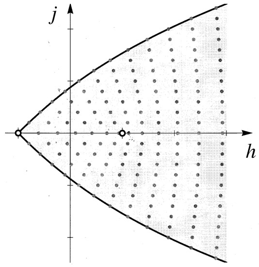
Figure 1. The Bohr–Sommerfeld quantum states of the spherical pendulum in $\overline{R}$.

The basic sections of the quantum line bundle $\pi :L\to T^{*}{S}^2$ are

$${\sigma }_{n,m}:T_{n,m}^2\subseteq T^{*}{S}^2\to L:({\vartheta }_1,{\vartheta }_2)\mapsto \left({\vartheta }_1,{\vartheta }_2,{\mathrm{e}}^{2\pi i(n{\vartheta }_1+m{\vartheta }_2)}\right).$$

The family of sections $\mathfrak{B}=\{{\sigma }_{n,m}\mid (n,m)\in {\mathbb{Z}}_{\ge 0}\times \mathbb{Z}\}$ forms a basis of quantum states of the Bohr–Sommerfeld theory of the spherical pendulum. Let $\mathfrak{H}$ be the Hilbert space of quantum states for which $\mathfrak{B}$ is an orthogonal basis. The Bohr–Sommerfeld energy momentum spectrum $\mathfrak{S}$ of the spherical pendulum is the range of the map

$$\begin{array}{c}{\mathcal{A}}_{\mid {\mathbb{Z}}_{\ge 0}\times \mathbb{Z}}^{-1}:{\mathbb{Z}}_{\ge 0}\times \mathbb{Z}\subseteq {\mathbb{R}}_{\ge 0}\times \mathbb{R}\to \overline{R}:\hfill \\ (n,m)\mapsto \left(h(n\mathrm{h},m\mathrm{h}),j(n\mathrm{h},m\mathrm{h})\right)=\left(h_m\left(n\right)ћ,mћ\right).\hfill \end{array}$$

$(n,m)\in {\mathbb{Z}}_{\ge 0}\times \mathbb{Z}$ are the quantum numbers of the spherical pendulum.

In terms of actions $A_1$ and $A_2$, we may write $H=H(A_1,A_2)$. Hence, the quantum operators $Q_H$ and $Q_J$ act on the basic sections ${\sigma }_{m.n}$ as follows

$$\begin{array}{cc}\hfill Q_H{\sigma }_{n,m}& =H_{\mid T_{n,m}^2}{\sigma }_{n,m}=h_m\left(n\right)ћ{\sigma }_{n,m}\hfill \end{array}$$

and

$$\begin{array}{cc}\hfill Q_J{\sigma }_{n,m}& =J_{\mid T_{n,m}^2}{\sigma }_{n,m}=mћ{\sigma }_{n,m}.\hfill \end{array}$$

The regular part of $T^{*}{S}^2$ is

$$S_0={\mathcal{EM}}^{-1}\left(R\right)={\mathcal{EM}}^{-1}\left({\mathcal{A}}^{-1}\left(\{{\mathcal{A}}_1>0\&{\mathcal{A}}_2\ne 0\}\right)\right).$$

The singular part of $T^{*}{S}^2$ consists of six strata:

$$\begin{array}{cc}\hfill S_1& ={\mathcal{EM}}^{-1}\left({\mathcal{A}}^{-1}(\left\{(0,0)\right\}\right),\hfill \\ \hfill S_2& =\left({\mathcal{A}}^{-1}(\left\{(4/\pi ,0)\right\}\right),\hfill \\ \hfill S_3& =({\mathcal{A}}^{-1}\left(\{({\mathcal{A}}_1,0)\mid 0<{\mathcal{A}}_1<4/\pi \}\right),\hfill \\ \hfill S_4& =({\mathcal{A}}^{-1}\left(\{({\mathcal{A}}_1,0)\mid 4/\pi <{\mathcal{A}}_1\}\right),\hfill \\ \hfill S_5& =({\mathcal{A}}^{-1}\left(\{(0,{\mathcal{A}}_2)\mid {\mathcal{A}}_2>0\}\right),\hfill \\ \hfill S_6& =({\mathcal{A}}^{-1}\left(\{(0,{\mathcal{A}}_2)\mid {\mathcal{A}}_2<0\}\right).\hfill \end{array}$$

The stratum $S_1$ is the point $(0,0,-1,0,0,0)\in T^{*}{S}^2$; while the stratum $S_2$ is the point $(0,0,1,0,0,0)$. The stratum $S_3$ is the subset of $T^{*}{S}^2$, where $A_1\in (0,4/\pi )$ and $A_2=0$, which is a cylinder parameterized by $(A_1,{\vartheta }_1)$; while $S_4$ is the subset where $A_1\in (4/\pi ,\infty )$ and $A_2=0$, which is a cylinder parameterized by $(A_1,{\vartheta }_1)$. The stratum $S_5$ is the subset of $T^{*}{S}^2$ where $A_1=0$ and $A_2>0$, which is a cylinder parameterized by $(A_2,{\vartheta }_2)$; while $S_6$ is the subset where $A_1=0$ and $A_2<0$, which is a cylinder parameterized by $(A_2,{\vartheta }_2)$.

The conditions of Corollary 1 are satisfied. For $i=1,2$ let $X_i=X_{{\vartheta }_i}$. In the regular stratum $S_0$ we get the shifting operators

$$\begin{array}{cc}\hfill {\mathbf{a}}_{X_1}{\sigma }_{n,m}& ={\sigma }_{n-1,m},\mathrm{provided} n>1 \mathrm{and} m\ne 0\hfill \\ \hfill {\mathbf{b}}_{X_1}{\sigma }_{n,m}& ={\sigma }_{n+1,m},\mathrm{provided} n>0 \mathrm{and} m\ne 0\hfill \\ \hfill {\mathbf{a}}_{X_2}{\sigma }_{n,m}& ={\sigma }_{n,m-1},\mathrm{provided} n>0 \mathrm{and} m\ne 1\hfill \\ \hfill {\mathbf{b}}_{X_2}{\sigma }_{n,m}& ={\sigma }_{n,m+1},\mathrm{provided} n>0 \mathrm{and} m\ne 0\hfill \end{array}$$

Arguing as in the example of the 2-d harmonic oscillator, we can extend the above relations to

$$\begin{array}{cc}\hfill {\mathbf{b}}_{X_1}{\sigma }_{0,m}& ={\sigma }_{1,m},\mathrm{provided} m\ne 0\hfill \\ \hfill {\mathbf{b}}_{X_2}{\sigma }_{n,0}& ={\sigma }_{n,1},\mathrm{provided} m\ne 0.\hfill \end{array}$$

In addition, we may assume that

$${\mathbf{a}}_{X_1}{\sigma }_{0,m}=0\mathrm{and}{\mathbf{a}}_{X_2}{\sigma }_{n,0}=0.$$

Since the are no global action angle coordinates, the action function ${\mathcal{A}}_1$ on R is multi-valued. After encircling the point $(1,0)$, the quantum number of the Bohr–Sommerfeld torus represented by the upper right hand vertex of the rectangle on the h-axis, see Figure 2, becomes the quantum number of the upper right hand vertex of the parallelogram formed by applying $M^T=\left(\begin{array}{cc}1& 1\\ 0& 1\end{array}\right)$ to the original rectangle, which is the transpose of the monodromy matrix M of the spherical pendulum.

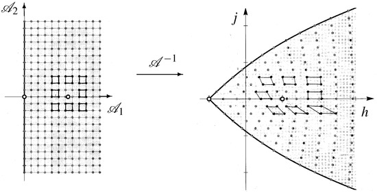
Figure 2. Using the shifting operators to show that the quantized spherical pendulum has monodromy.

The holonomy of the connection $\mathcal{E}$ is called the monodromy of the fibrating toral polarization D on $(P,\omega )$ with fibration $\rho :P\to B$.

Corollary 2.

Let $\tilde{B}$ be the universal covering space of B with covering map $\Pi :\tilde{B}\to B$. The monodromy map M, which is a nonidentity element holonomy group of the connection $\mathcal{E}$ on the bundle ρ sends one sheet of the universal covering space to another sheet.

Proof. 

Since the universal covering space $\tilde{B}$ of B is simply connected and we can pull back the symplectic manifold $(P,\omega )$ and the fibrating toral distribution D by the universal covering map to a symplectic manifold $(\tilde{P},\tilde{\omega })$ and a fibrating toral distribution $\tilde{D}$ with associated fibration $\tilde{\rho }:\tilde{P}\to \tilde{B}$. The connection $\mathcal{E}$ on the bundle $\rho$ pulls back to a connection $\tilde{\mathcal{E}}$ on the bundle $\tilde{\rho }$. Let $\gamma$ be a closed curve on B and let M be the holonomy of the connection $\mathcal{E}$ on B along $\gamma$. Then, $\gamma$ lifts to a curve $\tilde{\gamma }$ on $\tilde{B}$, which covers $\gamma$, that is, $\tilde{\rho }\circ \tilde{\gamma }=\gamma$. Thus, parallel transport of a k-torus $T={\mathbb{R}}^k/{\mathbb{Z}}^k$, which is an integral manifold of the distribution $\tilde{D}$, along the curve $\tilde{\gamma }$ gives a linear map M of the lattice ${\mathbb{Z}}^k$ defining the k-torus $M\left(\tilde{T}\right)$. The map M is the same as the linear map M of ${\mathbb{Z}}^k$ into itself given by parallel transporting T, using the connection $\mathcal{E}$, along the closed $\gamma$ on B because the connection $\tilde{\mathcal{E}}$ is the pull back of the connection $\mathcal{E}$ by the covering map $\rho$. The closed curve $\gamma$ in B represents an element of the fundamental group of B, which acts as a covering transformation on the universal covering space $\tilde{B}$ that permutes the sheets (= fibers) of the universal covering map $\tilde{\Pi }$. □

In the spherical pendulum, the universal covering space $\tilde{R}$ of $R\setminus \left\{\right(1,0\left)\right\}$ is ${\mathbb{R}}^2$. If we cut R by the line segment $\ell =\left\{\right(h,0)\in R\mid h>1\}$, then $R^{\times }=R\setminus \ell$ is simply connected and hence represents one sheet of the universal covering map of R. For more details on the universal covering map, see [22]. The curve chosen in the example has holonomy $M=\left(\begin{array}{cc}1& 1\\ 0& 1\end{array}\right)$. It gives a map of $\tilde{R}$ into itself, which sends $R^{\times }$ to the adjacent sheet of the covering map. Thus, we have a rule how the labelling of the Bohr–Sommerfeld torus $T_{(n_1,n_2)}$, corresponding to $(h,j)\in R^{\times }$, changes when we go to an adjacent sheet, which covers $R^{\times }$, namely, we apply the matrix M to the integer vector $\left(\begin{array}{c}{n}_1\\ n_2\end{array}\right)$. Since our chosen curve generates the fundamental group of $R\setminus \left\{\right(1,0\left)\right\}$, we know what the quantum numbers of Bohr–Sommerfeld are for any closed curve in $R\setminus \left\{\right(1,0\left)\right\}$, which encircles the origin.

References

- Heisenberg, W. Über die quantentheoretische Umdeutung kinematischer und mechanischer Beziehungen. Z. Phys. 1925, 33, 879–893. [Google Scholar] [CrossRef]
- Kostant, B. Quantization and unitary representations. I. Prequantization. In Lectures in Modern Analysis and Applications III; Lecture Notes in Mathematics; Springer: Berlin, Germany, 1970; Volume 170, pp. 87–208. [Google Scholar]
- Souriau, J.-M. Quantification géométrique. In Physique Quantique et Géométrie; Hermann: Paris, France, 1988; pp. 141–193. [Google Scholar]
- Blattner, R.J. Quantization in representation theory, In Harmonic Analysis on Homogeneous Spaces; Taam, E.T., Ed.; American Mathematical Society: Providence, RI, USA, 1973; Volume 26, pp. 146–165. [Google Scholar]
- Kobayashi, S.; Nomizu, K. Foundations of Differential Geometry; Interscience Publishers: New York, NY, USA, 1963; Volume 1. [Google Scholar]
- Souriau, J.-M. Structure des Systèmes Dynamiques; Dunod: Paris, France, 1970. [Google Scholar]
- Śniatycki, J. Geometric Quantization and Quantum Mechanics; Springer: New York, NY, USA, 1980. [Google Scholar]
- Dirac, P.A.M. Elimination of the nodes in quantum mechanics. Proc. Roy. Soc. A 1926, 111, 281–305. [Google Scholar]
- Cushman, R.; Śniatycki, J. Bohr-Sommerfeld-Heisenberg quantization of the 2-dimensional harmonic oscillator. arXiv 2012, arXiv:1207.1477v2. [Google Scholar]
- Cushman, R.; Śniatycki, J. On Bohr-Sommerfeld-Heisenberg quantization. J. Geom. Symmetry Phys. 2014, 35, 11–19. [Google Scholar]
- Cushman, R.; Śniatycki, J. Bohr-Sommerfeld-Heisenberg quantization of the mathematical pendulum. J. Geom. Mech. 2018, 10, 419–443. [Google Scholar] [CrossRef]
- Śniatycki, J. Lectures on geometric quantization. In Proceedings of the Seventeenth International Conference on Geometry, Integrability and Quantization, Varna, Bulgaria, 5–10 June 2015; Mladenov, I., Meng, G., Yoshioka, A., Eds.; Institute of Biophysics and Biomedical Engineering, Bulgarian Academy of Sciences. Avangard Prima: Sofia, Bulgaria, 2016; pp. 95–129. [Google Scholar]
- Sikorski, R. Abstract covariant derivative. Coll. Math. 1967, 18, 252–272. [Google Scholar] [CrossRef]
- Sikorski, R. Wstęp Do Geometrii Różniczkowej; PWN: Warszawa, Poland, 1972. [Google Scholar]
- Śniatycki, J. Differential Geometry of Singular Spaces and Reduction of Symmetry; Cambridge University Press: Cambridge, UK, 2013. [Google Scholar]
- Bohr, N. On the constitution of atoms and molecules (Part I). Philos. Mag. 1913, 26, 1–25. [Google Scholar] [CrossRef]
- Sommerfeld, A. Zur Theorie der Balmerschen Serie. Sitzungberichte der Bayerischen Akademie der Wissenschaften (München). Mathe-Matisch-Physikalische Klasse 1915. pp. 425–458. Available online: https://www.zobodat.at/pdf/Sitz-Ber-Akad-Muenchen-math-Kl_1915_0425-0458.pdf (accessed on 21 September 2020).
- Winnewisser, M.; Winnewisser, B.P.; Medvedev, I.R.; De Lucia, F.C.; Ross, S.C.; Bates, L.M. The hidden kernel of molecular quasi-linearity: Quantum monodromy. J. Mol. Struct. 2006, 798, 1–26. [Google Scholar] [CrossRef]
- Cushman, R.H.; Dullin, H.R.; Giacobbe, A.; Holm, D.D.; Joyeux, M.; Lynch, P.; Sadovskií, D.A.; Zhilinskií, B.I. CO2 Molecule as a quantum realization of the 1:1:2 resonant swing-spring with monodromy. Phys. Rev. Lett. 2004, 93, 024302. [Google Scholar] [CrossRef] [PubMed]
- Cushman, R.; Śniatycki, J. Classical and quantum spherical pendulum. arXiv 2016, arXiv:1603.00966v1. [Google Scholar]
- Cushman, R.H.; Bates, L.M. Global Aspects of Classical Integrable Systems, 2nd ed.; Birkhauser: Basel, Switzerland; Springer: Basel, Switzerland, 2015. [Google Scholar]
- Cushman, R.; Śniatycki, J. Globalization of a theorem of Horozov. Indag. Math. 2016, 26, 1030–1041. [Google Scholar] [CrossRef]
- Lukina, O.V.; Takens, F.; Broer, H.W. Global properties of integrable Hamiltonian systems. Reg. Chaotic Dyn. 2008, 13, 602–644. [Google Scholar] [CrossRef]
Publisher’s Note: MDPI stays neutral with regard to jurisdictional claims in published maps and institutional affiliations. |
© 2020 by the authors. Licensee MDPI, Basel, Switzerland. This article is an open access article distributed under the terms and conditions of the Creative Commons Attribution (CC BY) license (http://creativecommons.org/licenses/by/4.0/).