Abstract
Steering and suspension systems of a motor vehicle have very important mutual connections that have direct influence on a vehicle’s steerability, stability, comfort and life expectancy. These mechanical and functional couplings cause an intensive interaction between the two mentioned vehicle systems on a geometrical, kinematical and dynamical level. This article presents a study on nonparametric identification of dynamic interaction between the steering and the suspension system of a passenger vehicle. A specific methodology for experimental research in on-road conditions was designed that was in line with the research objectives and the applied measuring system. Experimental data were acquired for a curvilinear drive, with different constant driving speeds and on different roads. A multiple input/multiple output model for identification of the vehicle dynamics system from the aspect of interaction between the steering and the suspension system was developed. The analysis of experimental data was realized with the selection of a corresponding identification model, decoupling of model inputs and conditioned spectral analysis. The results of the conditioned spectral analysis of experimentally obtained data records indicate the level of interaction between the observed input and output parameters of the steering and the suspension systems to be in the frequency range below 30 Hz.
1. Introduction
Steering and suspension systems of motor vehicles are interconnected with especially important mechanical and functional connections that have direct influence on the vehicle’s steerability, stability, comfort and lifespan. Where vehicle dynamics is concerned, the term “stability” can be observed from several viewpoints. The most important type of stability of the solutions of differential equations of motion of the vehicle is the stability near the point of equilibrium described by the Lyapunov theory. In simple terms, the vehicle system is stable in the sense of Lyapunov if the solutions starting near to the equilibrium remain near forever. Vehicle stability is often observed in terms of “handling stability” or the vehicle’s ability to stabilize the direction of motion when disturbances affect the vehicle. Thus, the vehicle is considered as stable if it returns to a steady state and as unstable if it diverges from the desired trajectory even after disturbances disappear. Finally, stability of the vehicle can be observed from the aspects of overturning, sliding and cornering. When lateral vehicle stability is concerned, it is the stability in terms of vehicle motion in two cases: when the vehicle drives along a road with a transverse slope or when the vehicle is cornering on a horizontal road. In both cases, the vehicle can be unstable if lateral sliding or lateral overturn appears. Longitudinal vehicle stability implies the vehicle’s ability to move without overturning around the front or the rear axle and without slipping or sliding on the longitudinal slope.
Road excitations from a contact zone between the tires and the road are transferred through the wheels and the suspension system elements to the car body and the steering system. On the other hand, the driver turns the steering wheel and thus turns the steered wheels, causing changes in the kinematics of the steered wheels and the suspension system linkages. In order to maintain precise control over the vehicle, it is necessary to provide proper vehicle steerability. However, the vehicle steerability directly depends on the properties of the suspension system elements and proper geometry of the steered wheels, which are the elements of both the steering and the suspension systems of the vehicle. In practice, the steering and suspension systems of the vehicle should function as a single unit with harmonized geometrical, elasto-kinematic and dynamic parameters.
Research of the interaction between the steering and the suspension systems of the motor vehicle date back to the 1930s []. The original systems had evolved from purely mechanical to sophisticated active systems whose coordinated operation is controlled by integrated vehicle dynamics control systems. In this article, a brief review of research on phenomena directly or indirectly related to the interaction between the steering and the suspension systems in the last decade is given. The research in this area was mainly concentrated on finding the solutions to the following problems:
- occurrence of adverse effects that result from the interaction between the steering and the suspension systems,
- effects of design of the steering system and the suspension system on their interaction,
- solving the optimization problem of the steering and the suspension systems from the aspect of their interaction with the use of modern optimization methods and
- coordination of the steering and suspension systems operation via the integrated systems for vehicle dynamics control.
Very extensive research of the shimmy phenomenon in the steering system has been done, based on previously well-developed theory. Shimmy occurs at the front wheels of the vehicle with an independent suspension system in the form of self-sustained vibrations of the wheels about the steering axis. It is related to lateral compliance of the suspension and described as “violent and possibly dangerous vibration”, according to []. The same research sets the analytical models for investigation of shimmy of the systems with yaw and lateral degrees of freedom for both linear and nonlinear shimmy behavior.
Other undesirable effects of the influence of suspension deflection on vehicle steerability, such as “bump steer” and “roll steer”, were summarized and analytically expressed in []. “Bump steer” occurs in the steering system of a vehicle with an independent suspension system in the form of an additional steer angle that develops when the wheel changes its vertical position, with suspension bump deflection. When there is a difference in “bump steer” between the wheels of the same axle, the resulting motion is called “heave steer” or “double-bump steer”. “Roll steer” appears at the rigid axles in the form of a variation of steer of the axle (both wheels) when the car body rolls. Both effects are expressed with “steer coefficients” that relate the variation of the wheel steer angle to the corresponding excitation.
In research [,], the authors present a case study of the causes and the ways to reduce the “pull to side” effect during straight-line drive induced by suspension tolerances for a vehicle with front double wishbone suspension and rear five arms suspension. They used the design of experiments analysis and analysis of the vehicle assembly process to establish the effects of the difference between the front and rear axle slip angles and of the front camber angle on the “pull to side” phenomenon. The paper [] deals with the influence of the dimensional variations on the “pull to side”. The authors propose a method for evaluation of that influence for a vehicle with MacPherson front suspension and twist beam rear suspension systems.
The effects of the design of the steering system and the suspension system on their interaction have been investigated in literature at two levels. The first level presents the results of the impact the system exhibits as a whole, and the second level deals with the influence of a single or a group of steering and suspension parameters on the vehicle dynamic system.
In order to improve the steering parameters of the vehicle, the effects of new types of suspension systems were investigated. A new model of a planar suspension system with a longitudinal spring-damper element was investigated in [] with the aim to establish the influence of longitudinal compliance of the suspension on the vehicle handling. The results showed that the planar suspension system can successfully absorb the longitudinal bump-induced accelerations. In [], a control design for the steering system of an in-wheel electric vehicle coupled with a variable-geometry suspension system was investigated. The control system had a hierarchical architecture that enabled the modification of the camber angle and the scrub radius. Effects of the use of a hydraulically interconnected suspension system and an electronically controlled air spring on handling stability of a bus was investigated in []. Comparing the results of the on-road tests with the results of the vehicle multibody model, nonlinear air spring model and air spring fuzzy controller, the authors concluded that a bus equipped with the proposed suspension system might obtain “high performance for both handling stability and ride comfort” compared to a conventional bus.
The effects of the steering system geometry were researched in [] and the influence of both steering geometry and suspension parameters on ride comfort and road holding in [,]. The results showed that the cornering performance of a vehicle could be improved with controlling the camber angle of the front wheels []. A comparison of the experimental results, mechanics modelling and artificial neural network model of the influence of the steering performance parameters (king pin angle, steered wheel angles, scrub radius) and front suspension links length was presented in []. Relative quantification of the influence of steering geometry and suspension parameters was done in [], according to the results of the experimental test on a test rig and mathematical model formed by using design of experiments methods.
Influence of the reduced damping coefficient of the suspension system on the vehicle steering characteristics (understeer indicators, path radius to steer angle ratio, steering angle gradient) was investigated in []. The authors concluded that reduced damping causes an increase of vehicle understeer by 25% and of the steering wheel angle by 22° on the circle path and by 28° during dynamic steering angle change. The research [] deals with the influence of the suspension geometry parameters on the steering feedback. The authors investigated which geometric parameter was connected directly to the torque steer effect and concluded that “king pin offset has a strong influence on torque steer”.
The steering and the suspension systems of a vehicle should operate as a single system with the joint goal to maintain the desired handling performance, stability and ride quality. Often, these demands are conflicting and trade-off between them is necessary. This is achieved via the process of solving the optimization problem of the steering and the suspension systems parameters with regard to different objectives. Formulation of the optimization problem means the setting of mathematical equations and variables that describe the problem and comprise the following three components: an objective function, decision variables and constraints. The optimization algorithm aims to find the optimal solution to a problem in order to satisfy the objective function(s) subjected to constraints. Previous research was focused on the optimization of the parameters of the suspension system and the steering system separately, while newer research deals with the simultaneous optimization of both mentioned systems, using modern optimization methods.
In [], a genetic algorithm as a global search and optimization technique was used to optimize the control arm length, initial angle of the control arm and the initial angle of the strut of the McPherson suspension system for bump steer behavior, using three performance indices—variations of the toe angle, the camber angle and the caster angle. The multi-objective bees algorithm was used as the optimization method in [] to optimize the characteristic dimensions of the semi-trailing arm suspension using the “on-line” and “off-line” objective functions. The “off-line” objective function yields the solution with minimum variation of the camber angle, toe angle and wheel track, while the “on-line” objective function yields the solution with minimum variation of the wheel vertical reaction forces and minimum variation of the difference between the vertical forces at the front and the rear axles. The research presented in [] used a regularity model-based multi-objective estimation of distribution algorithm (RM-MEDA) combined with the design of experiments to optimize the passive vehicle suspension for ride and handling performance using eight objective and six constraint functions. Optimization of the suspension system in order to minimize the steering pull was investigated in [] using the robust design optimization method based on the radial basis function (RBF). The optimization problem was solved with the augmented Lagrange multiplier method. In [], kinematic characteristics of the suspension were optimized against the handling performance of the vehicle, using a robust 10-DOF mathematical model of the vehicle as the prediction model to optimize the front toe angle. Adams/Car software was used in order to optimize the suspension parameters using an iterative procedure to find the best design in []. Simultaneous optimization of the integrated electro-hydraulic power steering system and semi-active suspension system was done in [,]. Evaluation indexes for the observed steering system (steering energy loss, steering road feel, steering sensitivity) and for the observed suspension system (body acceleration, suspension dynamic disturbance and tire dynamic load) were introduced and the conclusion was reached that they have conflicting requirements. Thus, the optimization of the design was necessary, and it was achieved using the dynamic constraint analytical target cascading (DCATC) optimization method as the multi-level optimization method. Research [] presented the use of the real-code population-based incremental learning and differential evolution (RPBIL-DE) method for optimization of the steering system linkage in order to minimize the steering error and the turning radius, taking into account the effects of the front suspension. The research presented in [] has introduced the possibility for using a virtual test rig to improve in general any process of optimization of the steering and the suspension systems parameters.
Modern motor vehicles have various chassis control systems that work independently. In order to integrate their functions, avoid performance conflicts and achieve the common goals, various proposals for integrated vehicle dynamics control or global chassis control were made. Global chassis control systems enable simultaneous systems control, coordination between the operation of different vehicle control systems and sharing of information between various sensors and actuators []. Fundamentals and emerging concepts of an integrated vehicle dynamics control can be found in []. Research [] offers the integrated robust control design of the front wheel steering and the variable-geometry suspension system with the goal of the improvement of vehicle stability. In [], a nonlinear integrated system with a bilinear controller and a “human-vehicle function allocation module” with the task to enhance ride comfort and handling stability was elaborated on in detail. A three-layer hierarchical strategy for integrated control of an active suspension system, active front steering and a direct yaw moment was presented in [], while research [] offers a global vehicle control scheme containing a coordinated control strategy for active suspension, active front steering and differential braking systems.
A review of the above-mentioned research has shown that a relatively small number of articles deal directly with the issue of interaction between the steering system and the suspension system. The emphasis of research was placed on the determination of the parameters of the suspension system and the steered wheels that induce the oscillations in the steering system and on the available options for reducing the oscillations in the steering system. The impact of the steering system on the suspension system has not been sufficiently researched. Detailed mechanical models of tires, suspension systems and parts or complete steering systems are most often derived. Based on the laws of analytical mechanics, differential equations of motion are set and solved. Analytical considerations have rarely been followed by experimental tests on the test benches and on the experimental vehicle.
Since there are detailed dynamic models of the various combinations of steering systems and suspension systems, this article does not deal with the development of the mathematical-mechanical model. Instead, the development of the nonparametric model of the interaction between the steering and the suspension systems was researched. The main goal was to develop a universal nonparametric model for identification of interaction between different combinations of steering and suspension systems of various vehicles. The proposed nonparametric model from [] with six inputs (vertical accelerations at the centers of the wheels, steering wheel torque and steering wheel angle) and two outputs (vertical acceleration at the top of the front left shock absorber and the normal stress in the left tie-rod) was used to analyze the experimental results. The experimental records were obtained via on-road tests of an experimental passenger vehicle. The analysis of the autocorrelation functions, cross-correlation functions, cross-spectra and partial coherence functions were focused on the factors that influence the vibrational loads of the tie-rod in stationary and nonstationary driving conditions.
The research from [] has been extended and presented in this article. Experimental tests conducted on the vehicle in road conditions were aimed at determination of the influence of the vehicle speed, the type of road and the shape of the track on the interaction between the steering and the suspension systems. The tests were performed while driving at constant and variable speeds. The following types of roads were used: section of highway, asphalt roads in good, medium and bad condition and gravel road. The road tracks were rectilinear and curvilinear in shape. The results were analyzed in the frequency domain, using the newly developed software programs in the Matlab environment, intended for conditioned spectral analysis and the identification of frequency characteristics of the observed input-output transfer channels for stationary processes. Representative examples of the results of the conditioned spectral analysis for the tests performed during curvilinear driving with a constant speed are presented and analyzed in this article.
2. Materials and Methods
Methodologies of investigation of interaction between the steering and the suspension systems of the vehicle are not standardized. In this case, a purpose-built methodology was designed in accordance with the main goal of the research.
2.1. Experimental Investigations
Experimental investigations were conducted on a conventional passenger vehicle containing a rack and pinion hydraulic power steering system, a front McPherson strut suspension system and a twist beam rear suspension system. The front suspension system had lower lateral control arms and a stabilizer to connect both lower control arms of the front wheels.
A specific experimental system was designed and then used to identify the interaction between the vehicle steering and suspension systems. It consists of four basic groups of components: sensors, measuring amplifiers, data acquisition system and recording (computer) unit, Figure 1. The following quantities were measured in accordance with the goal of the research:
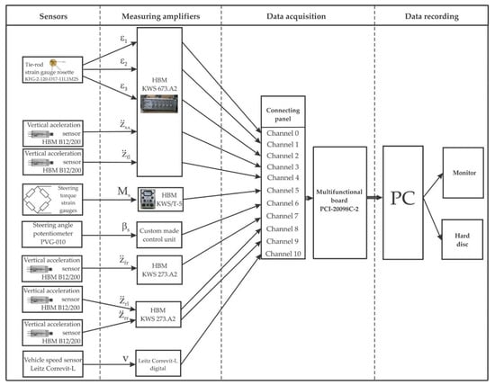
Figure 1.
Experimental system.
- steering wheel torque, Ms,
- steering wheel angle, βs,
- normal stress of the front left tie-rod, σn, indirectly measured through the relative deformations of the strain gauge rosette ε1, ε2, ε3, with the strain gauges placed in directions of 0/45°/90° in relation to the tie-rods axis, respectively,
- vertical accelerations at the centers of the wheels: front left, , front right, , rear left, , and rear right, ,
- vertical acceleration at the top of the left shock absorber, , and
- longitudinal vehicle speed, v.
The steering wheel torque and the steering wheel angle were measured using the sensors from the custom designed dynamometric steering wheel shown in Figure 2. The dynamometric steering wheel had replaced the original steering wheel of the vehicle. It was mounted by means of specially designed adapters and girders. Four strain gauges were used for indirect measurement of steering wheel torque. The gauges were mounted on the test tube (1), two at each side of the steering column, and then connected into the full Wheatstone bridge using a measuring amplifier (HBM, type KWS/T-5). The Wheatstone bridge circuit of the strain gauges was supplied with an AC voltage (carrier frequency excitation) from the measuring amplifier. The output signal of the bridge circuit was modulated on the carrier frequency as amplitude variation, so the output voltage was also an AC voltage. The output signal was demodulated in the measurement amplifier and then sent to the analogue filter with the cut-off frequency of 50 Hz. By measuring the bending moment of the test tube, the strain gauges measured the proportional steering wheel torque.
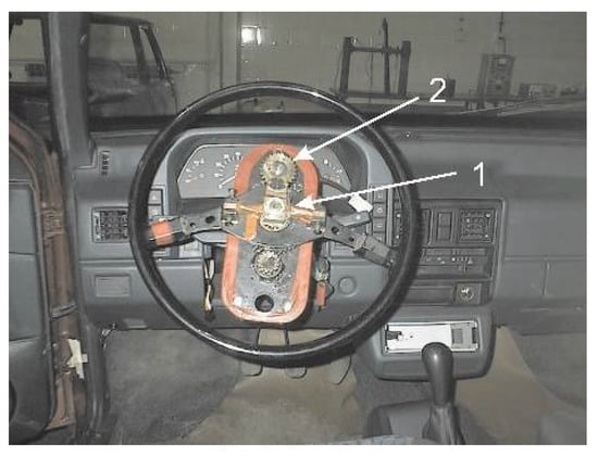
Figure 2.
Dynamometric steering wheel for measurement of the steering wheel torque and the steering wheel angle [].
The steering wheel angle was measured using a rotating potentiometer PVG-100 (2) mounted on the small shaft parallel to the steering column. It has a possibility to obtain 9 full revolutions. The potentiometer shaft is connected to the steering wheel column through the pair of gears with a gear ratio of 1:1.883. Rotation of the steering column transfers to the potentiometer shaft through the gears thus enabling the potentiometer to measure indirectly the angular displacement of the steering wheel.
The left tie-rod loads were measured with two miniature strain gauge rosettes (Omega Engineering, type KFG-2-120-D17-11L1M2S), Figure 3. The rosettes have an electric resistance of 120 kΩ and a K-factor of 2.08. The active rosette (1) was placed on a flat surface near the tie-rod joint to measure the tie-rod strain. The compensating rosette (2) was placed on a specially made metal ring. The support ring was not in direct contact with the body of the tie-rod, but through layers of elastic-plastic sealant Syntex 30. The compensating rosette was placed near the measuring rosette. Due to the elastic characteristics of the sealant, the compensating rosette was not exposed to the tie-rod strains. The rosettes were glued to the measuring points according to the rules for surface preparation and gluing of strain gauges. Each of the three strain gauges of the active rosette was connected with the corresponding strain gauge of the passive rosette to form the half-bridge connections, thus making the three input channels of the measuring amplifier.
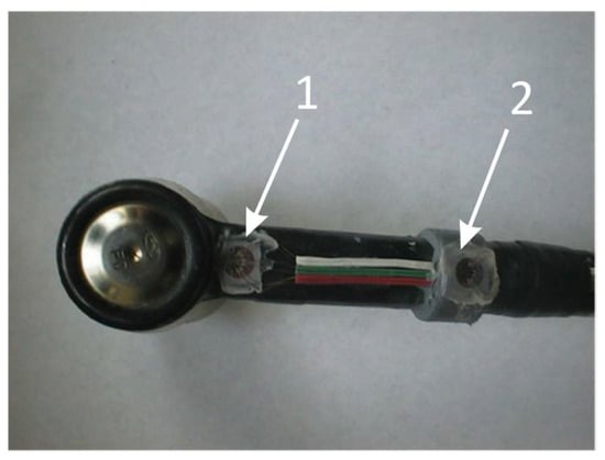
Figure 3.
Strain gauge rosettes for measurement of the tie-rod loads [].
Inductive acceleration sensors (HBM, type B12/200), shown in Figure 4, were used to measure the vertical accelerations at the centers of all four wheels and at the top of the front left shock absorber. They were mounted at measuring points using specially designed carriers. For the sensors of vertical acceleration of the wheels, it was important that they be placed as close to the wheel centers as possible and in a vertical direction. Here, the term “vertical acceleration” should be understood conditionally—the sensors are rigidly attached to the wheel hubs, so their movements are not performed only in the vertical direction. However, since the variations of the camber and the caster wheel angles are very small, the effects of the measurement direction were negligible.
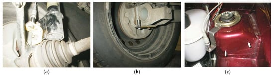
Figure 4.
Vertical acceleration sensors: (a) at the centers of the front wheels []; (b) at the centers of the rear wheels []; (c) at the top of the front left shock absorber.
The carriers of the vertical acceleration sensors at the centers of the front wheels were firmly bolted to the lower connections of the shock absorbers at the wheel hubs, Figure 4a. At the rear wheels, the carriers of the acceleration sensors were firmly bolted to the rear wheel hubs, Figure 4b.
The sensor that measures the vertical acceleration at the top of the front left shock absorber was mounted on a specially designed carrier that enabled its mounting in a vertical direction, Figure 4c. The carrier plate was firmly connected with the shock absorber carrier.
The correlation-optical sensor Leitz Correvit-L shown in Figure 5 was used to measure the vehicle longitudinal speed. The non-contact speed sensor Leitz Correvit L uses spatial frequency velocimetry technology based on illumination of the road surface and imaging of its micro-structure. The reflected light goes through optical grating to a photodiode. The cross-correlation of the road surface image moving over the grating leads to a signal frequency that is proportional to the vehicle velocity, thus the term “correlation-optical sensor”. Measuring range of this sensor is from 3 km·h−1 to 200 km·h−1. It needs a DC power supply in the range from 10 V to 16 V, which was provided by the vehicle main battery and the Leitz Correvit-L2 Digital device.
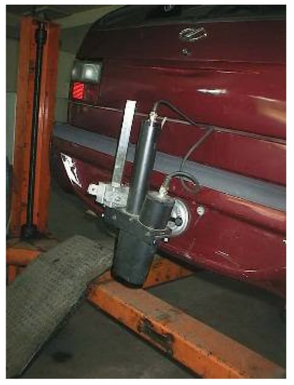
Figure 5.
Correlation-optical sensor for measurement of vehicle longitudinal speed.
2.2. Development of the Model for Identification of Interaction between the Steering and the Suspension Systems
There are two types of identification of the dynamic structure of a system:
- nonparametric identification or direct estimation of the impulse or frequency response of the system and
- parametric identification, in which a specific system structure is assumed, and the parameters of that structure are estimated on the basis of measured data (e.g., the “state-space” method).
Nonparametric identification is mostly used in the identification of systems in the frequency domain, where the system is often seen as a “black box”, without any assumptions about its nature. Therefore, nonparametric identification seems to be more applicable than parametric identification, which often requires that the analyzed data have a normal probability distribution. However, although more widely applicable, nonparametric identification requires a significantly larger amount of available data to achieve results with the same level of reliability as parametric identification.
In accordance with the main goal of this research, nonparametric identification was chosen for the identification of the vehicle dynamic system from the aspect of the interaction between the steering and the suspension system. For the purpose of conditioned spectral analysis, the assumption is introduced that the observed system is linear (additive and homogeneous). A significant feature of a linear system is that its impulse transfer function does not depend on the input. In addition, if the system is linear, random inputs with a Gaussian probability density function produce outputs with the same probability density function. In practice, linearity is a feature of the system that is most often compromised, especially with random inputs. In that case, there is a probability of the occurrence of the inputs being so extreme that the system can no longer respond proportionally to the input. However, unless the system is highly nonlinear, the analysis procedures used in [,] will give valid results in terms of the best linear approximations using the least squares method.
The processing of the experimentally obtained data was obtained in several phases:
- selection of the appropriate model,
- model verification,
- decoupling of the mutual influences of the inputs and
- conditioned spectral analysis.
The form of the preliminary adopted model for system identification depends mostly on the selected measured quantities that represent the inputs or the outputs of the system. Spectra of the measured input and output quantities can be used as inputs and outputs of the observed vehicle dynamic system dedicated to the conditioned spectral analysis of the system. However, the structure of this system may be unknown. When it comes to more complex tasks, such as identifying the interaction between the steering system and the suspension system of the vehicle, it is about observing vehicle dynamic systems with multiple inputs and multiple outputs.
The nonparametric model for spectral analysis of the vehicle dynamic system shown in Figure 6 was formulated according to the main goal of the research. The model has six arbitrary selected inputs and two outputs, Figure 6a.
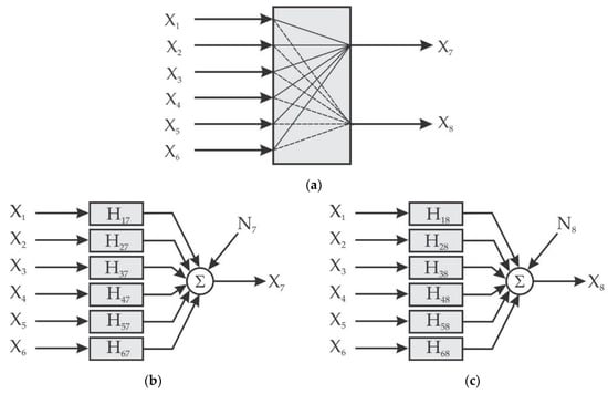
Figure 6.
Structure of the vehicle dynamic system model with six arbitrary inputs and two outputs. (a) General model of the system; (b) equivalent multiple input/single output model for the output ; (c) equivalent multiple input/single output model for the output .
The following spectra were used as arbitrary inputs to the nonparametric model:
- spectrum of vertical acceleration at the center of the front left wheel, ,
- spectrum of vertical acceleration at the center of the front right wheel, ,
- spectrum of vertical acceleration at the center of the rear left wheel, ,
- spectrum of vertical acceleration at the center of the rear right wheel, ,
- spectrum of the steering wheel torque, , and
- spectrum of the steering wheel angle, .
The adopted outputs of the model were:
- spectrum of vertical acceleration at the top of the front left shock absorber, , and
- spectrum of normal stress of the front left wheel tie-rod, .
Each input, , affects both outputs and through corresponding transfer channels characterized by optimum constant parameter linear frequency response functions, . In this case, the general model can be viewed as a combination of two multiple input/single output models shown in Figure 6b,c. Noise spectra, N7 and N8, shown in Figure 6b,c, correspond to the outputs X7 and X8, respectively, and represent all possible deviations from the linear models due to a small number of inputs, time delays, nonlinearities, statistical errors, non-stationarity, instrument noise, etc.
In order for the model to be correctly defined, the following four conditions must be met, which, in fact, determine the beginning of the system analysis [,]:
- No ordinary coherence function between any two inputs should be equal to unity. If this happens, one of the inputs should be removed from the model because it carries redundant information.
- No ordinary coherence function between any input and output should be equal to unity. If this is the case, then the other inputs practically do not contribute to the output of the model, so the model can be viewed as a model with single input and single output.
- The multiple coherence function between any input and other inputs, excluding a given input, must not be equal to unity, because then the given input is a linear combination of other inputs and should be ejected from the model.
- The multiple coherence function between the outputs and the given inputs should be high enough for the theoretical assumptions and conclusions to make sense. Otherwise, most likely, some inputs into the system have been omitted or the effects of nonlinearity of the system are very pronounced.
All necessary ordinary coherence functions and multiple coherence functions were calculated. It was established that no ordinary coherence function between the two inputs and between any input and output, as well as no multiple coherence function between any input and other inputs, excluding a given input, were equal to unity. The multiple coherence function between the outputs and the given inputs was high enough for the theoretical assumptions and conclusions to make sense. Hence, the conclusion that the system is correctly defined was justified.
Considering the required conditions and the fact that the multiple input/multiple output system can be observed as a combination of several equivalent multiple input/single output systems, the system model with arbitrary selected inputs from Figure 6 was replaced by alternative models—for the output , Figure 7a, and for the output , Figure 7b. The original inputs were decoupled using the conditioned spectral analysis and replaced by a set of ordered conditioned inputs,. The ordinary frequency response functions were replaced with optimal frequency response functions, , of the system with conditioned inputs. They are different from the frequency response functions of the system with arbitrary selected inputs. Spectra of the output noise for each output, and , and spectra of the two outputs, and , remained the same.
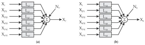
Figure 7.
Equivalent multiple input/single output models for conditional spectral analysis: (a) equivalent model for the output X7; (b) equivalent model for the output X8.
Theoretical aspects of conditioned spectral analysis are well known and comprehensively presented in [,], so they will not be elaborated in detail. Least square estimates were used for obtaining the optimum systems for unconditioned and conditioned inputs (described by optimal frequency response functions Hij and Lij, respectively), which minimize the auto-spectral density function of the output noise, Snn. Here, the optimum system is defined as a linear system which produces minimum mean square system error. The mentioned theory was used to formulate the algorithm for the conditioned spectral analysis of the experimental data in this particular case.
2.3. Algorithm for Conditioned Spectral Analysis
The algorithm for conditioned spectral analysis is presented for the example of the equivalent system shown in Figure 7a. It consists of several procedures. The analysis begins with calculations of the spectra of the inputs and the output, , via Fourier transforms. Then, the auto-spectra of the inputs and the output, , and the cross-spectra between the inputs and the output, , are calculated using the following expression, valid for a definite data record length of T:
Here, function E is the mathematical expectation function and is the complex conjugate of .
The algorithm continues with the procedure for alternate computation of optimal frequency response functions of the system with six conditioned (uncoupled) inputs, , conditioned cross-spectra of the inputs and the output, , and auto-spectrum of the output noise, , Equation (2).
The conditioned inputs from Figure 7a are denoted with . This means that the linear effects of the inputs from X1 to Xi−1 have been removed from the input Xi using optimal estimation techniques based on the least square method [,]. The ordered conditioned inputs are not mutually coupled (because the coupling effects caused by the dependence between the inputs were removed using the conditioned spectral analysis), which, in general case, does not apply to original inputs.
The conditioned uncoupled input spectra, , and the output noise spectrum are calculated according to the following procedure:
Frequency response functions of the initial system with the coupled inputs, , can be calculated (in the reverse order) using previously calculated optimal frequency response functions of the system with ordered conditioned inputs, :
Partial coherence functions between the conditioned inputs and the output, , are:
The multiple coherence function of the observed system, , is calculated as follows:
When the inputs are not correlated (as is the case with the model with conditioned inputs), the following expression is also valid for the multiple coherence function:
where are ordinary coherence functions between each input and the output of the system with arbitrary inputs:
Corresponding computer codes were developed for conditioned spectral analysis and visualization of the analysis results, based on the developed algorithm.
3. Results
The experimental vehicle equipped with the designed experimental system was driven on the road, with different speeds, road surface conditions and path shapes. The road tests were carried out in normal weather conditions during several consecutive summer days. The air temperature was around 25 °C and the relative air humidity was around 70%. The influence of crosswind was negligible. The vehicle was driven along the curvilinear sections of the road, with a constant speed and on dry road surfaces with high adhesion coefficients. The tires were inflated to the nominal inflation pressure. The static tire loads were the same for all the tests. The coefficients of adhesion were not directly measured or estimated. However, the described test conditions ensured the realization of small values of wheel slip and large values of the utilized adhesion coefficients at all wheels of the vehicle.
Data acquisition was performed with the Intelligent Instrumentation PCI-20000 data acquisition system, with a sampling frequency of f0 = 100 Hz and individual data record lengths of T = 30 s. The frequency range of the primary interest was set to 0 to 50 Hz. It is assumed that the processes under study are stationary and globally ergodic. Thus, their properties can be obtained properly on the basis of one realization. From a practical point of view, experiments are designed in such a manner that they produce stationary data. It is often achieved by maintaining constant experimental conditions, which is done in this case (the most significant constant condition being the constant vehicle speed). The measured experimental records were subjected to a nonparametric stationarity test and they proved to be stationary at the 5% level of significance.
Measurements are always associated with some kind of uncertainty. Measurement errors related to measurement equipment contain two components—systematic (instrumental, environmental, observational) or random.
To avoid instrumental errors, the measuring equipment was well maintained and calibrated at regular time intervals, according to the manufacturer’s recommendations. The setting of the instruments was performed (elimination of zero offset, checking the calibration) before every test. Environmental errors were minimized by keeping the environmental conditions (temperature, air pressure, humidity) as constant as possible and via protection of the equipment from the effects of electromagnetic fields. Observational errors were avoided via the use of the digital instruments for calibration and measurement, which eliminated reading errors of the operators.
Random errors mainly occur due to the limitations of the measuring instruments. Some of the declared accuracy parameters of the measuring equipment were the following:
- HBM KWS measuring amplifiers had an accuracy class of 0.1,
- calibration unit HBM K3602 for calibration of the strain gauge measuring amplifier had an accuracy class of 0.5,
- inductive acceleration sensors HBM B12/200 had relative error up to ±0.2% and
- Leitz Correvit speed sensor had measuring accuracy of ±0.1%.
The dynamometric steering wheel was custom built and data on the measuring accuracy of the implemented sensors for the steering wheel torque and the steering wheel angular position were not available.
The first step in processing was to remove the eventual nonzero mean values and periodicities. Calibration charts were used to transfer voltage units into corresponding physical units. In order to check whether the adopted model for identification of the vehicle dynamic system from the aspect of interaction between the steering and the suspension system was defined correctly, and the ordinary coherence functions between all inputs and between each input and each output were calculated. The values of coherence between the inputs have shown that there was a certain correlation between inputs, indicating the need to decouple the inputs before the data analysis. The inputs were reordered according to the magnitude of ordinary coherence functions, starting from the input giving the highest magnitude. None of the ordinary coherence functions between the inputs were equal to unity, so none of the inputs carried redundant information. All the coherence functions between each input and each output were not equal to unity, so all the inputs contributed to the output(s) of the model.
The multiple coherence functions between inputs and all other inputs excluding the given input were not equal to unity, meaning that individual inputs were not the linear combination of the other inputs. The multiple coherence functions for both outputs were sufficiently high, so the conclusions drawn from the analysis were meaningful.
The examples of the experimental results and the results of the analysis will be presented for the experimental records obtained from the vehicle driving along a curvilinear path on medium quality asphalt road, with a constant speed of v = 40 km∙h−1.
3.1. Example of the Results for the Conditioned Spectral Analysis
The original inputs of the model were decoupled and values for the conditioned inputs were calculated. Figure 8 shows the magnitudes of spectra of all conditioned inputs. Magnitudes of conditioned spectra of vertical accelerations at the centers of the wheels, Figure 8a–d, obtain their peak levels for the frequencies that coincide with the usual eigenfrequencies of the unsuspended masses for all wheels (8 Hz to 15 Hz). In addition, the tires behave as the selective filters that pass certain excitation frequencies from the road roughness, depending on tire dimensions, vehicle speed and the type of the road (the wavelength of the road roughness).
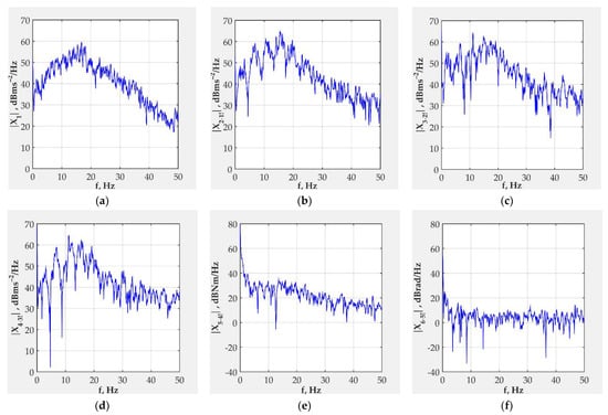
Figure 8.
Magnitudes of spectra of ordered (decoupled) inputs: (a) ; (b) ; (c) ; (d) ; (e) ; (f) .
Magnitudes of the conditioned spectra of the steering wheel torque, Figure 8e, and the steering wheel angle, Figure 8f, obtain their maximum values in the low frequency range and then sharply decrease.
The outputs of the system have magnitudes of the spectra presented in Figure 9. These magnitudes are equal to the magnitudes of the original output spectra of the system. The magnitude of the spectrum of the vertical acceleration at the top of the shock absorber, , Figure 9a, shows peaks at the frequencies of 1.9 Hz and 9.4 Hz. The magnitude of spectra decreases with the frequency because the suspension system acts like “a filter” that attenuates high frequency vibrations and prevents their transmission to the suspended mass. The magnitude of spectrum of the normal stress in the tie-rod, , has a distinctive peak value at 1.9 Hz and continuously decreases with the increase in frequency, Figure 9b. This means that the vibrations of the suspended mass influence the vibration behavior of the steering system. The magnitude of this spectrum rapidly decreases with the frequency.
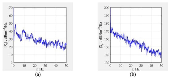
Figure 9.
Magnitudes of output spectra: (a) ; (b) .
Figure 10 presents magnitudes of noise spectra for both outputs—vertical acceleration at the top of the shock absorber, Figure 10a, and the normal stress of the tie-rod, Figure 10b. It should be noted that the output noise could not be controlled, because it originates from nonlinearities of the system and the contributions from eventual unmeasured inputs. The output noise spectrum is uncorrelated with the ordered conditioned inputs. The magnitudes of the two observed output noise spectra decrease with the increase in frequency.
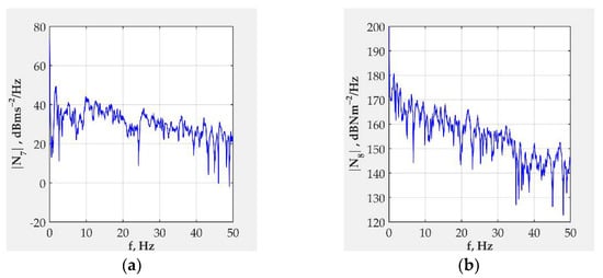
Figure 10.
Magnitudes of output noise spectra: (a) ; (b) .
The optimum linear frequency response functions, , for the outputs and are shown in Figure 11 and Figure 12, respectively. These functions can be used to locate system resonances and estimate system damping. The peak values of the optimal frequency response functions point to the natural frequencies of the system.
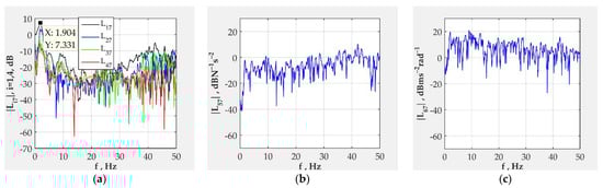
Figure 11.
Magnitudes of optimal frequency response functions for the transfer channels: (a) ; (b) ; (c) .
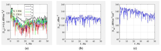
Figure 12.
Magnitudes of optimal frequency response functions for the transfer channels: (a) ;(b) ; (c) .
Figure 11a presents comparative values of the optimum frequency response functions of the transfer channels “vertical acceleration at the wheel—vertical acceleration at the top of the shock absorber”. All frequency response functions have distinctive peak values at the frequencies of 1.9 Hz and 9.4 Hz. These frequencies are the eigenfrequencies of the unsuspended and suspended masses, respectively. The magnitudes decrease from the peak value at 9.4 Hz to a frequency of around 25 Hz because of the suspension system damping. Then, they slightly increase for the frequencies up to 50 Hz, with a distinctive peak value at 42.5 Hz. Vertical acceleration at the center of the front left wheel has the largest influence on the vertical acceleration at the top of the front left shock absorber (the largest values of optimum frequency function). This is a logical consequence of the near placement of the two corresponding vertical acceleration sensors and mechanical coupling between measuring points.
The same peak value at a frequency of 42.5 Hz occurs in magnitudes of the optimum frequency response functions of the transfer channels between the steering wheel torque and the steering wheel angle as inputs and vertical acceleration at the top of the shock absorber, Figure 11b,c, respectively. This implies that an element of the system resonates at the mentioned frequency. The magnitude of the frequency response function of the channel “steering wheel torque—acceleration at the top of the shock absorber” gradually increases with the increase of frequency. Conversely, the magnitude of the frequency response function of the channel “steering wheel angle—acceleration at the top of the shock absorber” decreases with the increase of frequency.
The magnitudes of optimum frequency functions for the transfer channels between the vertical accelerations at the centers of all four wheels and the normal stress in the cross section, Figure 12a, have a mutual peak value at a frequency of 1.9 Hz. They slowly decrease to a frequency of around 20 Hz and then fluctuate until the end of the frequency range. This means that vertical accelerations affect the normal stress of the tie-rod in the low frequency range.
According to the magnitude of the optimal frequency response function shown in Figure 12b, the steering wheel torque exhibits a constant influence on the normal stress in the cross section of the left tie-rod. This is the expected consequence of the direct mechanical coupling between the steering wheel and the front left tie-rod. The magnitude of the optimal frequency response function for the channel “steering wheel angle—normal stress in the tie-rod” decreases with the increase of frequency up to 30 Hz. After that, this influence is negligible.
Figure 13 and Figure 14 present the values of partial coherence functions of all inputs for the output —vertical acceleration at the top of the shock absorber—and for the output —normal stress in the cross-section of the tie-rod.
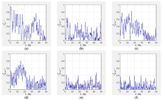
Figure 13.
Partial coherence functions between the conditioned inputs and the output for the transfer channels: (a) ; (b) ; (c) ; (d) ; (e) ; (f) .
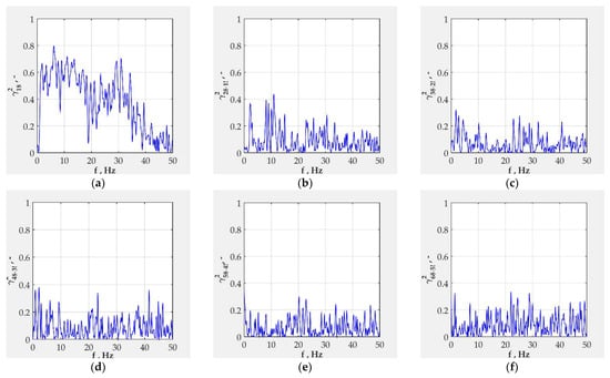
Figure 14.
Partial coherence functions between the conditioned inputs and the output for the transfer channels: (a) ; (b) ; (c) ; (d) ; (e) ; (f) .
The greatest values of the partial coherence functions are obtained for input —vertical acceleration at the center of the front left wheel—and both outputs (Figure 13a and Figure 14a). This is the obvious consequence of the fact that there is a direct physical connection between the center of the front left wheel and the connection point between the shock absorber and the car body and the front left tie-rod. Vertical accelerations at the centers of other wheels, Figure 13b–d and Figure 14b–d, exhibit smaller influence on both outputs, especially on the normal stress in the cross section of the tie-rod.
The steering wheel torque, Figure 13e and Figure 14e, and the steering wheel angle, Figure 13f and Figure 14f, produce the lowest values of partial coherence functions for both outputs. These values are smaller than 0.4, so this indicates that there is a weak connection between the mentioned inputs and the outputs. This may be the consequence of the fact that the steering wheel torque and the steering wheel angle have insufficient “spectral strength” in the observed frequency range.
The multiple coherence functions between the outputs and and the set of all inputs are presented in Figure 15a,b, respectively. They measure the extent to which the outputs may be predicted from the given inputs. Values of multiple coherence functions for vertical acceleration at the top of the shock absorber as output and all the inputs are very high (between 0.8 and 0.98) in the frequency range from 0 to 35 Hz. This means that the output vertical acceleration at the top of the shock absorber may be reliably predicted in the mentioned frequency range by the model from Figure 7a.
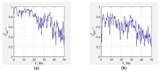
Figure 15.
Multiple coherence functions between the conditioned inputs and the output: (a) ; (b) .
The model from Figure 7b provides smaller but sufficient values of multiple coherence function ranging from 0.6 to 0.8 in the frequency range between 0 and 35 Hz. These smaller values suggest that the model from Figure 7b may be improved by introduction of some other inputs.
Ordinary coherence functions from Figure 16 and Figure 17 indicate how much of the outputs and , respectively, originate from each input. These functions are used to measure the degree of linear connection between the outputs and the inputs.
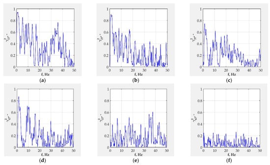
Figure 16.
Ordinary coherence functions between the inputs and the output for the transfer channels: (a) ; (b) ; (c) ; (d) ; (e) ; (f) .
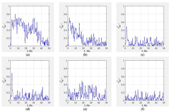
Figure 17.
Ordinary coherence functions between the inputs and the output for the transfer channels: (a) ; (b) ; (c) ; (d) ; (e) ; (f) .
For all inputs except the steering wheel angle, the values of ordinary coherence functions from Figure 16a–e and from Figure 17a–e have values between 0 and 1. This means that the mentioned inputs and outputs are partially linearly connected. The sources of nonlinearity encompass the measurement noise, nonlinear relations between inputs and outputs and the existence of other possible inputs not contained in the adopted models.
The coherence functions between both outputs and the steering wheel angle, Figure 16f and Figure 17f, are closer to zero across the entire frequency range. This may be a consequence of the low spectral content of the steering wheel angle at the higher frequencies. In addition, this may also indicate a problem with the data acquisition.
The magnitudes of the optimum frequency functions of the system with the coupled inputs from Figure 6, , are presented in Figure 18 and Figure 19, for the outputs and , respectively.
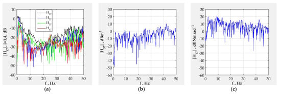
Figure 18.
Magnitudes of ordinary frequency functions between the inputs and the output for the transfer channels: (a) ; (b) ; (c) .
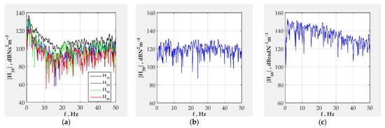
Figure 19.
Magnitudes of ordinary frequency functions between the inputs and the output for the transfer channels: (a) ; (b) ; (c) .
Optimum frequency functions of the system with the coupled inputs minimize the noise at the output. The same observations stated for the optimum frequency response functions for the system with the conditioned inputs are valid here.
3.2. Effects of the Vehicle Speed
Effects of the vehicle speed are illustrated for a curvilinear drive over the medium quality asphalt road with constant vehicle speeds of 40 km·h−1 and 60 km·h−1. Diagrams for the most influential input—vertical acceleration at the front left wheel, —are given in Figure 20.
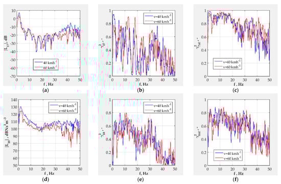
Figure 20.
Effects of vehicle speed on: (a) magnitude of frequency response function ; (b) partial coherence function ; (c) multiple coherence function ; (d) magnitude of frequency response function ; (e) partial coherence function ; (f) multiple coherence function .
Vehicle speed affects the magnitudes of optimum frequency response functions shown for the transfer channel , Figure 20a, and the transfer channel , Figure 20d. It appears that the smaller speed induces greater magnitude values. This is especially pronounced for the transfer channel in the observed frequency range. The transfer channel has a frequency range between 5 Hz and 30 Hz, in which the higher speed induces greater values of the magnitudes. This occurrence should be further examined.
Diagrams of the partial coherence functions and , Figure 20b,d, illustrate the portion of the outputs caused by the input —vertical acceleration at the front left wheel. The basic shapes of the partial coherence curves for transfer channels and are the same for the two vehicle speeds. The large variance of the results prevents the drawing of the conclusions related to the influence of speed on the level of coherence. In addition, values of the partial coherence function for the transfer channel have large fluctuations. The influence of the vertical acceleration at the center of front left wheel is considerable in the range between 0 and 30 Hz.
The curves of multiple coherence functions for transfer channels and , Figure 20c,f, respectively, show that higher speed induces higher values of multiple coherence functions for both observed transfer channels. The values of the multiple coherence functions also indicate that the adopted models from Figure 7a,b are best suited for the frequency range from 0 to 30 Hz.
3.3. Effects of the Road Quality
Effects of the road quality are presented for the case of curvilinear driving along the medium quality and good quality asphalt roads with the constant speed of 60 km·h−1. Again, diagrams for the most influential input—vertical acceleration at the front left wheel, —are given in Figure 21.
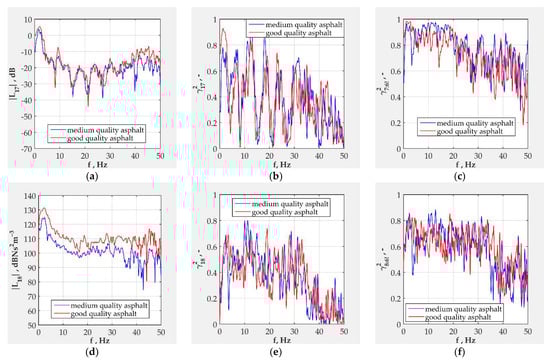
Figure 21.
Effects of road quality on: (a) magnitude of frequency response function ; (b) partial coherence function ; (c) multiple coherence function ; (d) magnitude of frequency response function ; (e) partial coherence function ; (f) multiple coherence function .
Driving along the better quality asphalt roads induces overall larger magnitudes of the optimal frequency response functions for both transfer channels, , Figure 21b, and , Figure 21e. The influence of the type of road is more pronounced for the transfer channel .
The curve shapes of the ordinary coherence functions and their values for both transfer channels remain the same, regardless of the type of road, Figure 21b,e. The values of the ordinary coherence function for the channel have large fluctuations. A large variance of the values prevents the drawing of definite conclusions regarding the influence of the road quality.
Multiple coherence functions for the transfer channel , Figure 21c, indicate that better quality road slightly reduces its values. The values are considerably high in the frequency range from 0 to 30 Hz. The multiple coherence function for the channel , Figure 21f, remains almost constant (at the mean value around 0.7) in the frequency range between 0 and 35 Hz, then drops to smaller values (at the mean value around 0.4).
4. Discussion
Conducted experimental tests and conditional spectral analysis have shown that there exists an interaction between the steering system and the suspension system of a vehicle at a geometrical, kinematical and dynamical level. The multiple coherence functions between the outputs and the inputs of the model are high enough for conclusions to make sense. According to the adopted model for conditioned spectral analysis, selected inputs are correlated because the values of all ordinary coherence functions between the inputs were between 0 and 1. This means that the inputs must have been decoupled before the conditional spectral analysis was conducted. The magnitudes of the optimal frequency response functions between the inputs and output show that it is best to use the adopted model in a frequency range from 0 to 30 Hz.
The input vertical accelerations at the wheel centers have a high influence on the outputs (vertical acceleration at the top of the shock absorber and the normal stress in the tie-rod), measured using the magnitude of the corresponding ordinary coherence functions. Vertical accelerations at the centers of the wheels represent the equivalent measurable excitation of the vehicle systems due to the road roughness.
Considering the magnitudes of the optimal frequency functions for the channels relating the vertical accelerations at the centers of the wheels (as inputs) and the two given outputs, it can be observed that the vertical acceleration at the center of the front left wheel has the greatest influence on both outputs. The observed statistical unreliability of some of the results in the frequency range over 30 Hz should be attributed to unfavorable signal-to-noise ratio at the outputs of the model.
Vehicle longitudinal speed as a controllable factor affects the intensity of the observed frequency response functions. The magnitudes of the frequency response functions decrease with the increase of vehicle longitudinal speed. On the contrary, the increase of vehicle longitudinal speed brings higher values of multiple coherence functions between the outputs and all inputs.
Road quality also affects the frequency response functions. Better quality roads increase the magnitudes of the frequency response functions. The influence of the road quality is not so obvious for the ordinary and multiple coherence functions.
It is obvious from the presented relationships of the adopted system that the steering wheel torque and the steering wheel angle spectra do not have necessary levels and frequency content in the observed frequency range between 0 and 50 Hz in real operating conditions. In other words, during the experiment, the steering wheel should be turned in such a way as to excite all eigenfrequencies of the system and the generated signal should have constant spectral density in the observed frequency range. It should be noted that ideal shapes of the signals from the steering wheel could not be achieved in real experimental conditions due to driver limitations. This implies that the robot steering wheels may be used in order to generate the “white noise” spectra with sufficient frequency content.
The level of the detected output noise indicates that introduction of some other inputs should be taken into account. The experimental system should be completed with additional inputs such as normal load of the right tie-rod, the loads of the suspension elastic elements and the shock absorbers at the front wheels and lateral acceleration of the vehicle coupled with the yaw angle. In that case, presented investigations, predominantly directed at the vehicle vertical dynamics, will be extended to the lateral vehicle dynamic.
The logical extension of the selected model would be the introduction of variable speed, making the model non-stationary. This means the introduction of the theory of random non-stationary processes, which is significantly more complex.
As a result of the spectral analysis, the nonparametric model was identified in the form of discrete values of frequency characteristics. The shape of the frequency characteristics indicates the structure of the observed transfer channel. The parameters of the frequency characteristics may be significant for investigations that are more complex. In that case, nonparametric model should be complemented with the corresponding parametric model.
Author Contributions
Conceptualization, D.M.; methodology, D.M.; software, D.M and J.G.; validation, D.M. and J.L.; formal analysis, J.L. and J.G.; investigation, D.M. and N.M.; resources, D.M.; data curation, D.M.; writing—original draft preparation, D.M.; writing—review and editing, J.L., J.G. and N.M.; visualization, N.M. and J.G.; supervision, J.L.; project administration, J.L. All authors have read and agreed to the published version of the manuscript.
Funding
This research was funded by the Ministry for education, science and technological development of the Government of the Republic of Serbia, grant number TR35041. The APC was funded by the authors of the article.
Data Availability Statement
The data is available through the corresponding author’s e-mail, at the reasonably explained request, and with the permission of the authors.
Acknowledgments
The ministry for education, science and technological development of the Government of the Republic of Serbia supported the research presented in the article (grant number TR35041).
Conflicts of Interest
The authors declare no conflict of interest.
Nomenclature
| steering wheel angle | |
| spectrum of the steering wheel angle | |
| ordinary coherence functions between each input and the output X7 of the system with arbitrary inputs | |
| partial coherence functions between the conditioned inputs and the output X7 | |
| multiple coherence function of the observed system with output X7 | |
| relative deformations of the strain gauge rosette, in directions of 0/45°/90°, respectively | |
| normal stress of the front left tie-rod | |
| spectrum of normal stress of the front left wheel tie-rod | |
| f0 | sampling frequency |
| optimal constant parameter linear frequency response functions of the original system(s) | |
| optimal frequency response functions of the conditioned system(s) | |
| magnitude of frequency response function of the channel | |
| magnitude of frequency response function of the channel | |
| Ms | steering wheel torque |
| spectrum of the steering wheel torque | |
| noise spectrum at the output X7 | |
| noise spectrum at the output X8 | |
| auto-spectra of the inputs and the output X7 | |
| cross-spectra between the inputs and the output X7 | |
| conditioned cross-spectra of the inputs and the output X7 | |
| auto-spectrum of the output noise at the output X7 | |
| T | data record length |
| v | vehicle speed |
| spectra of the inputs of the original system | |
| X7 | spectrum of the output vertical acceleration at the top of the shock absorber |
| magnitude of the spectrum of the vertical acceleration at the top of the shock absorber | |
| X8 | spectrum of the output normal stress of the tie-rod |
| magnitude of the spectrum of the normal stress in the tie-rod | |
| complex conjugate of Xi | |
| vertical accelerations at the center of the front left wheel | |
| spectrum of vertical acceleration at the center of the front left wheel | |
| vertical accelerations at the center of the front right wheel | |
| spectrum of vertical acceleration at the center of the front right wheel | |
| vertical accelerations at the center of the rear left wheel | |
| spectrum of vertical acceleration at the center of the rear left wheel | |
| vertical accelerations at the center of the rear right wheel | |
| spectrum of vertical acceleration at the center of the rear right wheel | |
| vertical acceleration at the top of the left shock absorber | |
| spectrum of vertical acceleration at the top of the front left shock absorber |
References
- Yang, S.; Lu, Y.; Li, S. An overview on vehicle dynamics. Int. J. Dynam. Control 2013, 1, 385–395. [Google Scholar] [CrossRef] [Green Version]
- Pacejka, H. Tyre and Vehicle Dynamics, 3rd ed.; Butterworth-Heinemann: Oxford, UK, 2012; pp. 287–328. [Google Scholar] [CrossRef]
- Dixon, J.C. Suspension Geometry and Computation, 1st ed.; John Wiley & Sons: Chichester, UK, 2009; pp. 127–141. [Google Scholar]
- De Rosa, M.; De Felice, A.; Fragassa, S.; Sorrentino, S. Passenger car steering pull and drift reduction considering suspension tolerances. In IOP Conference Series: Materials Science and Engineering, Proceedings of the 9th International Scientific Conference—Research and Development of Mechanical Elements and Systems (IRMES 2019), Kragujevac, Serbia, 5–6 September 2019; Marjanović, N., Ed.; IOP Publishing: Bristol, UK, 2019; Volume 012076, pp. 1–8. [Google Scholar]
- De Rosa, M.; De Felice, A.; Grosso, P.; Sorrentino, S. Straight Path Handling Anomalies of Passenger Cars Induced by Suspension Component and Assembly Tolerances. Int. J. Automot. Mech. Eng. 2019, 16, 6844–6858. [Google Scholar] [CrossRef]
- Muraria, T.B.; Lima, D.M.; Zebende, G.F.; Moret, M.A. Vehicle steering pull: From product development to manufacturing. Prod. Manag. Dev. 2016, 14, 22–31. [Google Scholar] [CrossRef]
- Zhu, J.J.; Khajepour, A.; Esmailzadeh, E. Handling transient response of a vehicle with a planar suspension system. Proc. Inst. Mech. Eng. Part D J. Aut. Eng. 2011, 225, 1445–1461. [Google Scholar] [CrossRef]
- Nemeth, B.; Fenyes, D.; Gaspar, P. Independent wheel steering control design based on variable-geometry suspension. IFAC-PapersOnLine 2016, 49, 426–431. [Google Scholar] [CrossRef]
- Qi, H.; Chen, Y.; Zhang, N.; Zhang, B.; Wang, D.; Tan, B. Improvement of both handling stability and ride comfort of a vehicle via coupled hydraulically interconnected suspension and electronic controlled air spring. Proc. Inst. Mech. Eng. Part D J. Aut. 2020, 234, 552–571. [Google Scholar] [CrossRef]
- Park, S.; Sohn, J. Effects of camber angle control of front suspension on vehicle dynamic behaviors. J. Mech. Sci. Technol. 2012, 26, 307–313. [Google Scholar] [CrossRef]
- Belkhode, P.N.; Mahalle, A.M.; Holay, P.P. Comparison of Steering Geometry Parameters of Front Suspension of Automobile. Int. J. Sci. Eng. Res. 2012, 3, I04–I06. [Google Scholar]
- Kiranchand, G.R.; Tanushri, S.; Mitra, A.C. Experimental Design, Sensitivity Analysis of Steering Geometry and Suspension Parameters. Mater. Today Proc. 2018, 5, 5743–5756. [Google Scholar] [CrossRef]
- Parczewski, K.; Wnek, H. Analysis of the impact of reduced damping in the suspension on selected vehicle steering characteristics. Proc. Inst. Mech. Eng. Part I J. Sys. 2019, 233, 392–399. [Google Scholar] [CrossRef]
- Bonera, E.; Gadola, M.; Chindamo, D.; Morbioli, S.; Magri, P. On the Influence of Suspension Geometry on Steering Feedback. Appl. Sci. 2020, 10, 4297. [Google Scholar] [CrossRef]
- Habibi, H.; Shirazi, K.H.; O’Connor, W.J. Optimization of the bump steering response of a McPherson suspension using a generic algorithm. In Multibody Dynamics—Computational Methods and Applications, Proceedings of the Conference Multibody Dynamics 2011, ECCOMAS Thematic Conference, Brussels, Belgium, 4–7 July 2011; Samin, J.C., Fisette, P., Eds.; ECCOMAS: Paris, France, 2011. [Google Scholar]
- Kazemi, M.; Shirazi, K.H.; Ghanbarzadeh, A. Optimization of semi-trailing arm suspension for improving handling and stability of passenger car. Proc. Inst. Mech. Eng. Part K J. Multi-Body Dyn. 2012, 226, 108–121. [Google Scholar] [CrossRef]
- Yuen, T.J.; Rahizar, R.; Mohd Azman, Z.A.; Anuar, A.; Afandi, D. Design Optimization of Full Vehicle Suspension Based on Ride and Handling Performance. In Lecture Notes in Electrical Engineering, Proceedings of the FISITA 2012 World Automotive Congress, Beijing, China, 27–30 November 2013; Springer: Berlin/Heidelberg, Germany, 2013; Volume 195, pp. 75–86. [Google Scholar] [CrossRef]
- Park, K.; Heo, S.J.; Kang, D.O.; Jeong, J.I.; Yi, J.H.; Lee, J.H.; Kim, K.W. Robust design optimization of suspension system considering steering pull reduction. Int. J. Automot. Techn. 2013, 14, 927–933. [Google Scholar] [CrossRef]
- Yuen, T.J.; Foong, S.M.; Ramli, R. Optimized suspension kinematic profiles for handling performance using 10-degree-of-freedom vehicle model. Proc. Inst. Mech. Eng. Part K J. Mul. 2014, 228, 82–99. [Google Scholar] [CrossRef]
- Ansara, A.S.; William, A.M.; Aziz, M.A.; Shafik, P.N. Optimization of Front Suspension and Steering Parameters of an Off-road Car using Adams/Car Simulation. Int. J. Eng. Res. Technol. 2017, 6, 104–108. [Google Scholar]
- Cui, T.; Zhao, W.; Wang, C.; Guo, Y.; Zheng, H. Design optimization of a steering and suspension integrated system based on dynamic constraint analytical target cascading method. Struct. Multidiscip. Optim. 2020, 62, 419–437. [Google Scholar] [CrossRef]
- Zhao, W.; Wang, C.; Zhao, T.; Li, Y. Research on the multi-disciplinary design method for an integrated automotive steering and suspension system. Proc. Inst. Mech. Eng. Part D J. Aut. 2015, 229, 1249–1262. [Google Scholar] [CrossRef]
- Sleesongsom, S.; Bureera, S. Optimization of Steering Linkage Including the Effect of McPherson Strut Front Suspension. In International Conference on Swarm Intelligence; Springer: Berlin/Heidelberg, Germany, 2018; Volume 10941, pp. 612–623. [Google Scholar] [CrossRef]
- Mantaras, D.A.; Luque, P. Virtual test rig to improve the design and optimisation process of the vehicle steering and suspension systems. Veh. Syst. Dyn. 2012, 50, 1563–1584. [Google Scholar] [CrossRef]
- Vivas-Lopez, C.A.; Tudon-Martinez, J.C.; Hernandez-Alcantara, D.; Morales-Menendez, R. Global Chassis Control System Using Suspension, Steering, and Braking Subsystems. Math. Probl. Eng. 2015, 2015, 263424. [Google Scholar] [CrossRef] [Green Version]
- Chen, W.; Xiao, H.; Wang, Q.; Zhao, L.; Zhu, M. Integrated Vehicle Dynamics and Control, 1st ed.; John Wiley & Sons: Singapore, 2016; pp. 201–338. [Google Scholar]
- Balazs, N.; Gaspar, P. Control design based on the integration of steering and suspension systems. In Proceedings of the 2012 IEEE International Conference on Control Applications (CCA), Dubrovnik, Croatia, 3–5 October 2012; pp. 382–387. [Google Scholar] [CrossRef]
- Wang, H.; Yang, L.; Hu, Y. Vehicle suspension and steering nonlinear integrated system coordinated control based on human-vehicle function allocation. In Proceedings of the 43rd International Congress on Noise Control Engineering (Inter Noise 2014), Melbourne, Australia, 16–19 November 2014. [Google Scholar]
- Zhao, J.; Wong, P.K.; Ma, X.; Xie, Z. Chassis integrated control for active suspension, active front steering and direct yaw moment systems using hierarchical strategy. Veh. Syst. Dyn. 2017, 55, 72–103. [Google Scholar] [CrossRef]
- Termous, H.; Shraim, H.; Talj, R.; Francis, C.; Charara, A. Coordinated control strategies for active steering, differential braking and active suspension for vehicle stability, handling and safety improvement. Veh. Syst. Dyn. 2018, 57, 1494–1529. [Google Scholar] [CrossRef]
- Demić, M.; Miloradović, D.; Glišović, J. A contribution to research of vibrational loads of the vehicle steering system’s tie-rod in characteristic exploitation conditions. J. Low. Freq. Noise Vib. Act. Control 2012, 31, 105–122. [Google Scholar] [CrossRef]
- Bendat, J.S.; Piersol, A.G. Random Data—Analysis and Measurement Procedures, 4th ed.; John Wiley & Sons: Hoboken, NJ, USA, 2010; pp. 201–247. [Google Scholar]
- Bendat, J.S.; Piersol, A.G. Engineering Applications of Correlation and Spectral Analysis, 2nd ed.; John Wiley & Sons: Hoboken, NJ, USA, 1980; pp. 188–234. [Google Scholar]
Publisher’s Note: MDPI stays neutral with regard to jurisdictional claims in published maps and institutional affiliations. |
© 2022 by the authors. Licensee MDPI, Basel, Switzerland. This article is an open access article distributed under the terms and conditions of the Creative Commons Attribution (CC BY) license (https://creativecommons.org/licenses/by/4.0/).