Article

Robust Velocity and Load Observer for a General Noisy Rotating Machine

by
Carlos Aguilar-Ibanez
1,*,†,
Manuel A. Jimenez-Lizarraga
2,†,
Isaac Gandarilla-Esparza
3,†,
Javier Moreno-Valenzuela
3,†,
Belem Saldivar
4,†,
Miguel S. Suarez-Castanon
5,† and
Jose de Jesus Rubio
6,†
1
Centro de Investigación en Computación, Instituto Politécnico Nacional, Ciudad de México 07738, Mexico
2
Facultad de Ciencias Físico Matemáticas, Universidad Autónoma de Nuevo León, Nuevo León 66451, Mexico
3
Centro de Investigación y Desarrollo de Tecnología Digital, Instituto Politécnico Nacional, Baja California 22430, Mexico
4
Departamento de Control Automático, CINVESTAV, Ciudad de México 07360, Mexico
5
Escuela Superior de Cómputo, Instituto Politécnico Nacional, Ciudad de México 07738, Mexico
6
Escuela Superior de Ingeniería Mecánica y Eléctrica Unidad Azcapotzalco, Instituto Politécnico Nacional, Ciudad de México 02550, Mexico
*
Author to whom correspondence should be addressed.
These authors contributed equally to this work.
Machines 2022, 10(11), 1009; https://doi.org/10.3390/machines10111009
Submission received: 7 September 2022 / Revised: 25 October 2022 / Accepted: 26 October 2022 / Published: 1 November 2022
(This article belongs to the Section Automation and Control Systems)

Abstract

:
This paper is focused on the design of a nonlinear observer for a rotatory machine with noise-affected output. It is assumed that the system is subject to bounded perturbations, and the original linear model of the machine is reformulated as a nonlinear system to include the desired signals to be estimated, namely, the velocity and load torque. The proposed observer leverages the so-called algebraic state-dependent Riccati equation to provide a robust estimation. Lyapunov analysis guarantees the convergence of the estimation error to a “ κ zone”. The proposed observer’s effectiveness is assessed through convincing numerical simulations and real-time experiments.

1. Introduction

Estimating the velocity and the load torque of a rotatory machine affected by noise that corrupts available measurements is an important problem in engineering applications.
Nowadays, there is an important need to reduce the costs of measuring instruments such as tachometers and external motor loads or torque sensors in rotating machines. In fact, a speed encoder is undesirable in a drive because it involves cost and reliability problems and sometimes even requires shaft extension and mounting arrangements [1]. While load and torque sensors are particularly costly, they are nevertheless necessary to recover information on the device’s interaction with the environment. This environment often presents disturbances in the load and velocities that make the control problem even more challenging, as lacking this information may severely decrease the control performance; see [2,3,4,5,6] for example. Connected with this, there is the problem of the periodic fluctuations in velocity in the rotating shaft, which introduce important errors that affect the performance of the general rotodynamic applications; see [7,8]. More recent works that can be found in the literature dealing with the problem of load torque estimation in cases considering noise include [9,10,11,12,13,14,15]. Nonetheless, these approaches are different from the solution proposed in this paper. Typically, the load torque in certain instances may be unknown, as pointed out in [16]. Estimation of such perturbed variables has been investigated in several research papers; for instance, see [1,16,17,18,19,20].
In [20], a novel method for estimating the motor load torque was proposed to reduce the cost associated with torque sensors. In [16], a rotor speed observer was designed for controlling a motor without a speed sensor. In [18], a performance and robustness comparison among three different algorithms for estimating the external load torque for low-power DC motors was presented. In [19], a sensorless online algebraic approach for the estimation of the load torque of a DC motor was proposed and compared with the sensorless reduced-order observer approach, with simulation and experimental results confirming the superiority of the proposed approach. In [17], the estimation of the disturbance torque in a sensorless DC motor drive was carried out by extending the classical observer theory; three estimation schemes were formulated according to the representation of the disturbance torque and the processing of the observer states. In [1], a solution based on the Immersion and Invariance (I&I) technique was proposed to solve the speed observer problem for a general rotating machine.
It is worth mentioning that simultaneous estimation of variables in a noisy environment is seen as a robust observation problem; see, for instance, [1,21,22,23]. There is extensive literature regarding the design of nonlinear observers for nonlinear systems affected by disturbances as well; see [24,25,26,27]. Different approaches are found in previous works for different scenarios. One of the most popular is the so-called high-gain observer [28,29,30,31], with an algorithm that reassembles the original nonlinear system plus an error correction term based on the available output. A matrix gain is included, and the challenge lies in finding the gain value that guarantees asymptotic convergence, commonly by Lyapunov methods. Additionally, in this context, the active disturbance rejection control approach arises as a tool for actual control of uncertain systems [32,33,34]. The sliding mode technique is another important proposal applied for the observation problem [35,36,37,38]. The resulting standard sliding mode observer retains the structure of the high-gain observer while exploiting the use of the discontinuous sign function in the correction term, allowing convergence to the “sliding error surface” in finite time. Although this approach works well, the discontinuous function introduces undesirable situations, such as the chattering effect. Adaptive observation is a third concept often found in the literature [39]. The underlying idea relies on the design of an observer with a nonlinear gain which continuously adapts to guarantee a bounded and convergent observation error. Adaptation observers may include dynamic neural networks, which might not require online training, as shown in [40].
To the best of the authors’ knowledge, none of the previous works have considered an approach for the simultaneous estimation of load and velocity affected by this type of noise based on the SDRE method, only bounded noise; the advantage of the proposed approach is the simplicity of the design, as by the suitable selection of the gain observer (stability analysis) the convergence of the estimation process to a zone can be guaranteed. This last claim in this paper is supported by numerical simulations and validated with real-time experiments. On the other hand, such an approach avoids the observer design challenges found in previous proposals, such as discontinuous functions [10,12,35,36], which may lead to undesired high-frequency oscillations; the need for high-order derivatives or integration, with the corresponding numerical complications [9]; the knowledge of statistical distribution for the noise [11], which is not always available; and not considering disturbances on measurements [1,17,20], passivity assumptions on the system [15,19,32], or the stability issues of adaptive procedures [16,24].
In this paper, the problem of observation of the linear model for the rotating machine is reformulated following the ideas presented in [1]. As a result, a nonlinear system is obtained in which the output is actually the velocity and the load torque to be estimated. The nonlinear system is then rearranged into a quasi-linear form while keeping the observability properties of the resulting system (see [41]). This allows exploiting the technique of the state-dependent Riccati equation in the observer design. The contributions of this paper are summarized as follows.
  • The original machine model is represented by a disturbed quasi-linear state-dependent model that preserves observability properties through transformations and provides the velocity and load torque as the output.
  • A quasi-linear state-dependent observer structure is designed.
  • Through Lyapunov analysis, the conditions to guarantee convergence to a “ κ zone” are determined.
  • Two numerical simulations and two real-time experiments are developed, showing the effectiveness of the proposed observer.
It is worth mentioning that the obtained disturbed quasi-linear state-dependent model does not consider certain important influence factors for the velocity and the load torque of the rotatory machine. Among these factors, the imperfections found in the support-bearing raceway and the lubricating characteristics have a major impact on the dynamical behavior of this kind of machine. A detailed treatment of these issues is beyond the scope of this study; however, the authors suggest the remarkable works [42,43], where these topics are deeply studied.
The rest of this paper is organized as follows. Section 2 presents the estimation problem statement and develops the necessary transformations to represent the original model as a quasi-linear perturbed one. In Section 3, the nonlinear observer is designed, and the Lyapunov analysis to ensure convergence on average to a specified zone is carried out. Section 4 and Section 5 present, respectively, numerical simulations and results of the real-time experiments validating the observer scheme. Finally, Section 6 is devoted to concluding remarks.

2. Problem Statement

To establish the observation problem, consider the rotating machine’s dynamic model defined by the set of differential equations provided by
θ ˙ = w , J w ˙ = k w + τ τ L + ζ ,
where the machine’s angular position and velocity are θ and w, respectively, the electromagnetic torque τ is the system input, τ L is the load torque, ζ represents additive bounded perturbations, and the system’s constant inertia and friction coefficient are denoted by J and k, respectively.
The observer’s objective is to estimate the speed w and the load torque τ L provided that J and k are known and position θ is available for measurement. It is worth mentioning that the difficulty in designing the observer arises from the fact that even when system (1) is linear, its state ( θ , w ) is defined in S × R , where S is a cylinder. Evidently, it is more convenient to define the measurable output as
y = y 1 y 2 = sin θ cos θ
and the new variable
z = z 1 z 2 = w τ L J
Consequently, replacing these new coordinates in system (1) and considering that z ˙ 2 = 0 , the following new representation is obtained:
z ˙ = A z + B τ + ζ 1 y ˙ = Ψ ( y ) z
where
A = k J 1 0 0 ; B = 1 J 0 ; ζ 1 = 1 J ζ 0 ; Ψ ( y ) = y 2 0 y 1 0 ;
From the above, the estimation objectives of this study can be rigorously introduced. Note that Equation (4) can be seen as an alternative model of the mechanical equations, where the actual outputs are defined according to (2).
Estimation problem: design an observer for the non-available velocity of system (4), assuming that the output y is measurable and the constants J and k are known. The state estimation error is defined as the difference between the state estimation vector and the actual state vector, e = x ^ x , and the goal is to achieve the upper bound defined in (5):
lim sup T 1 T t = 0 T e Q 0 2 d t C e < .
This is the state estimation error given the output measurement, which remains bounded on average. This is a good expectation, considering the existence of the perturbation.
It must be stressed that even when the stated control problem seems easy to solve, it is not. To the best knowledge of the authors, only a single solution has been previously published, in [1]. In that study, the variable z was estimated using an I&I-based reduced-order observer, an output filter, and a single dynamic scaling parameter. Note that the I&I-based reduced-order observer follows verbatim the procedure developed in [44,45]. In this contribution, a practical solution is proposed by assuming that the control model and the measurable output are externally perturbed. This solution combines the traditional LQR theory and the linear control theory known as the SDRE approach. To this end, the control model (4) is rewritten as
x ˙ = F ( x ) + B e τ + ξ 1
where x = [ y 1 , y 2 , z 1 , z 2 ] T and
F ( x ) = y 2 z 1 y 1 z 1 k J z 1 z 2 0 ; B e = 0 0 1 J 0 ; ξ 1 = 0 0 1 J ζ 0 .
where the single perturbation ξ 1 acts on the mechanical model. By adding the perturbation ξ 2 to the measurable output y , the complexity of the control problem under consideration is increased. In this case, the output is provided by
y = Cx + ξ 2
where ξ 2 and C are defined as
ξ 2 = ξ 11 ξ 12 ; C T = 1 0 0 1 0 0 0 0 .
Finally, it is easy to see that the stated observation problem differs from the one proposed in [1]; here, the uncertain and unmeasurable control model output is considered. The considered control model can be described by Equation (9):
x ˙ = F ( x ) + B e τ + ξ 1 y = Cx + ξ 2

3. Design of the SDRE Observer

The state-dependent Riccati equation (SDRE) method is a systematic approach for nonlinear control system design [41,46] which has been naturally extended to estimation problems. This method is applied by writing the nonlinear system (6) in the state-dependent coefficient form as
x ˙ = A e ( x ) x + B e τ + ξ 1
where F ( x ) = A e ( x ) x . Evidently, this parameterization for a continuous A e ( x ) is possible if F ( 0 ) = 0 and F ( x ) C 1 [46,47]. However, as discussed in [48], even if F is only continuous finding a continuous factorization is possible, though not guaranteed. It should be noted that this parameterization is not unique in the multivariable case. For this particular case, the matrix A e can be selected as
A e ( x ) = 0 z 1 2 y 2 2 0 z 1 2 0 y 1 2 0 0 0 k J 1 0 0 0 0
Therefore, an observer for system (10) can be proposed as
x ^ ˙ = A e ( x ^ ) x ^ + B e τ + L ( y C x ^ ) y ^ = C x ^
The challenge at this point is to find a matrix L that guarantees a finite upper bound for the average quadratic error for the noisy dynamics.
Remark 1.
A condition for the solution of equation (12) is that the par { A e ( x ^ ) , C } must be continuously locally observable for all times t, or at least at each discrete instant t; that is, the rank of the observability test matrix [49]
O = C : CA e 3
must be 4. For this case, the condition is satisfied if w 0 (see Appendix A). All this means that if the motor angular velocity is equal to zero, the load torque τ L cannot be estimated.
Throughout this paper, the following assumptions are considered valid.
  • Assumption 1 The parameterization of matrix A e satisfies the Lipschitz condition globally, that is, there exists L f > 0 such that
    A e x + e A e x L f e
    for any x and e R 4 .
    The proof of this assumption can be found in Appendix A.
  • Assumption 2 : The noises or disturbances are bounded:
    ξ 1 ε 1 ξ 2 ε 2
  • Assumption 3 : The gain matrices K and LC produce a positive solution 0 < P = P R n × n of the following state-dependent matrix equation:
    PK + K P + PRP + Q = 0
    where
    K = A e x LC ; R = Λ 1 + Λ 2 + Λ 3 ; Q = ε 3 2 Λ 3 1 L f 2 I + Q 0
    for some positive matrices Q 0 and Λ 1 + Λ 2 + Λ 3 , that is,
    0 < Q 0 = Q 0 R n × n ; 0 < Λ = Λ R n × n ; Λ = Λ 1 , Λ 2 , Λ 3
  • Assumption 4 : The system and the observer states are bounded:
    x σ ; x ^ ε 3
    Please note that assumptions 1–4 are common in the SDRE theory; in particular, they hold for the considered model, as can be verified in the proofs of assumptions 1 and 2 provided in Appendix A.
Theorem 1.
If, for a nonlinear model (12), assumptions 1–4 hold, then the ’on average’ error convergence to a κ−zone is guaranteed:
e Pe κ t 0 ,
where
κ = β γ ; γ : = λ min P 1 / 2 Q 0 P 1 / 2 β : = L Λ 1 1 L ε 1 2 + Λ 2 1 ε 2 2
Proof. 
Define the estimation error as e = x ^ x . The time-derivative of the error is provided by
e ˙ = x ^ ˙ x ˙ = A e x ^ x ^ A e x x + L Cx C x ^ + L ξ 2 ξ 1 + A e x A e x x ^ = A e x e LCe + L ξ 2 ξ 1 + A e x ^ A e x x ^ = A e x LC e + L ξ 2 ξ 1 + A e e + x A e x x ^ .
Note that the error dynamics fulfills the following equation:
e ˙ = A e ( x ) LC e + ϕ ( x , x ^ ) ,
where
ϕ ( x , x ^ ) = L ξ 2 ξ 1 + A e e + x A e x x ^ .
Defining the Lyapunov function as V e = e P 2 : = e Pe yields
d d t V e = 2 e P A e x LC e + L ξ 2 ξ 1 + A e e + x A e x x ^ .
Using the matrix inequality
X Y + Y X X Λ X + Y Λ 1 Y
and Assumptions 1–4, it is easy to see that the following set of inequalities are fulfilled:
d d t V e e PK + K P e + e P Λ 1 + Λ 2 + Λ 3 Pe + ξ 2 L Λ 1 1 L ξ 2 + ξ 1 Λ 2 1 ξ 1 + A e e + x A e x x ^ Λ 3 1 2 e PK + K P + P Λ 1 + Λ 2 + Λ 3 P + Q 0 e e Q 0 e + L Λ 1 1 L ε 1 2 + Λ 2 1 ε 2 2 + Λ 3 1 L f 2 e 2 ε 3 2 e PK + K P + P Λ 1 + Λ 2 + Λ 3 P + ε 3 2 Λ 3 1 L f 2 I + Q 0 e e P 1 / 2 P 1 / 2 Q 0 P 1 / 2 P 1 / 2 e e P 1 / 2 P 1 / 2 Q 0 P 1 / 2 P 1 / 2 e + β λ min P 1 / 2 Q 0 P 1 / 2 e Pe + β
where the constant β is defined above. This last inequality allows us to establish the statement of the theorem. □

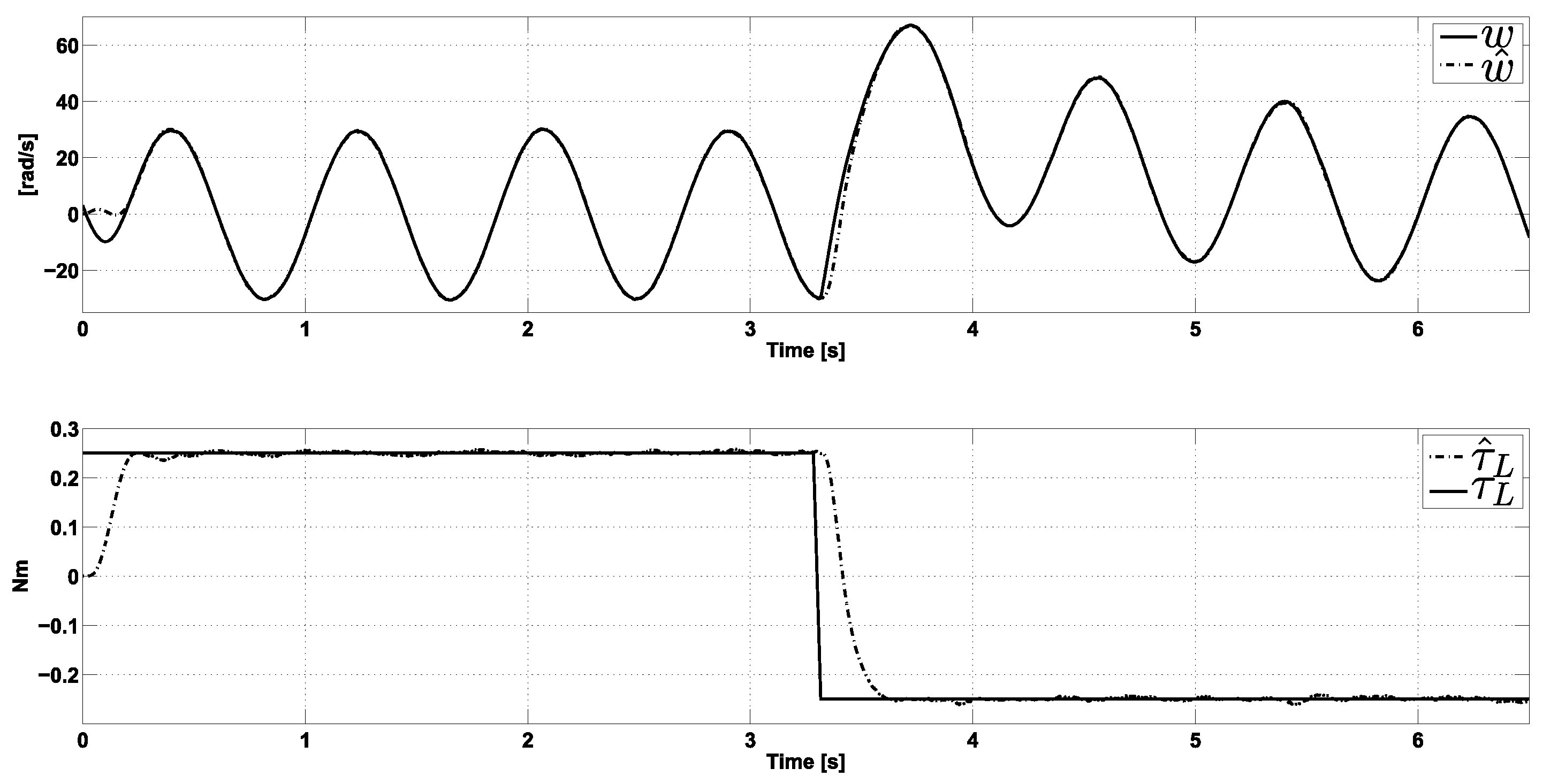
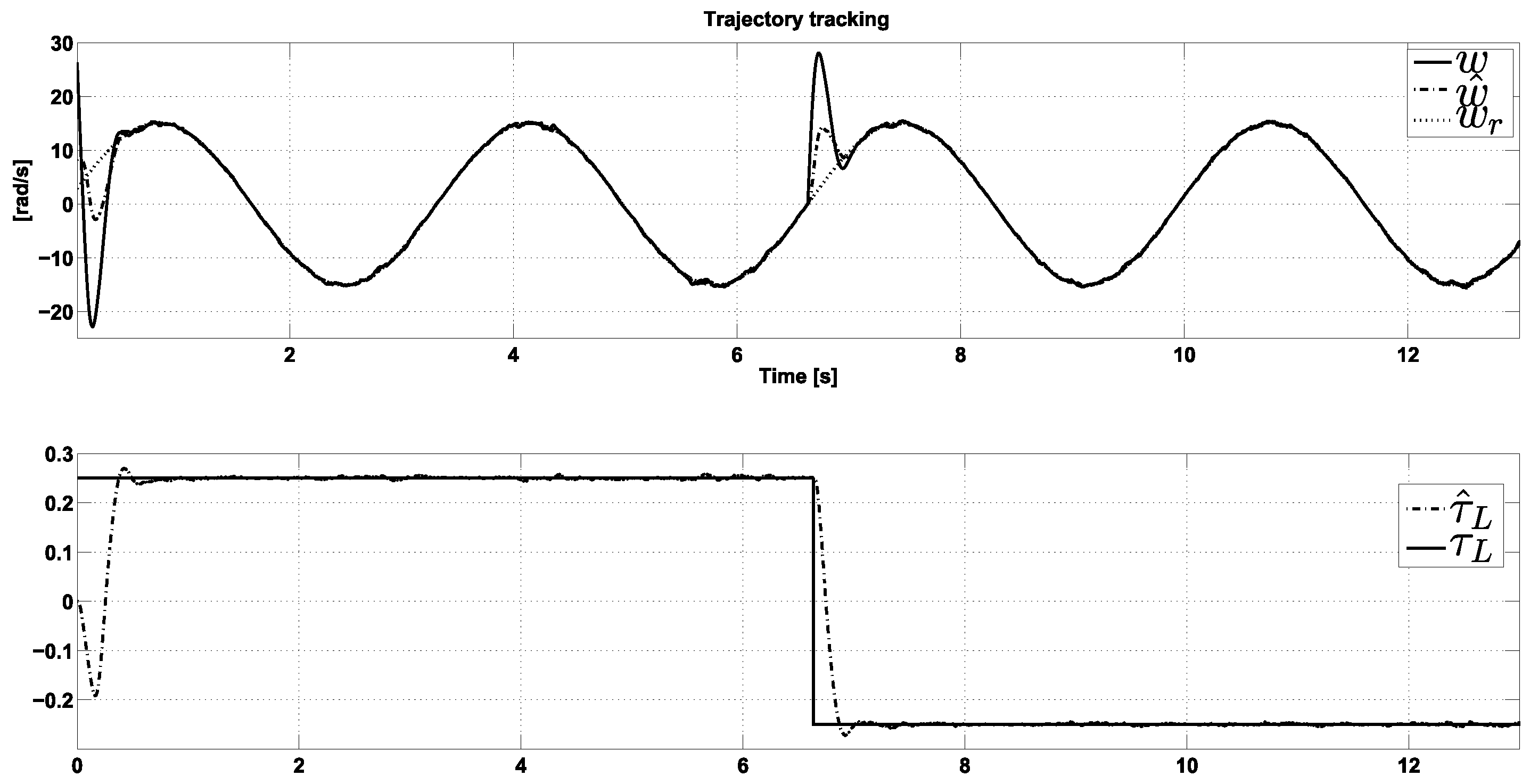
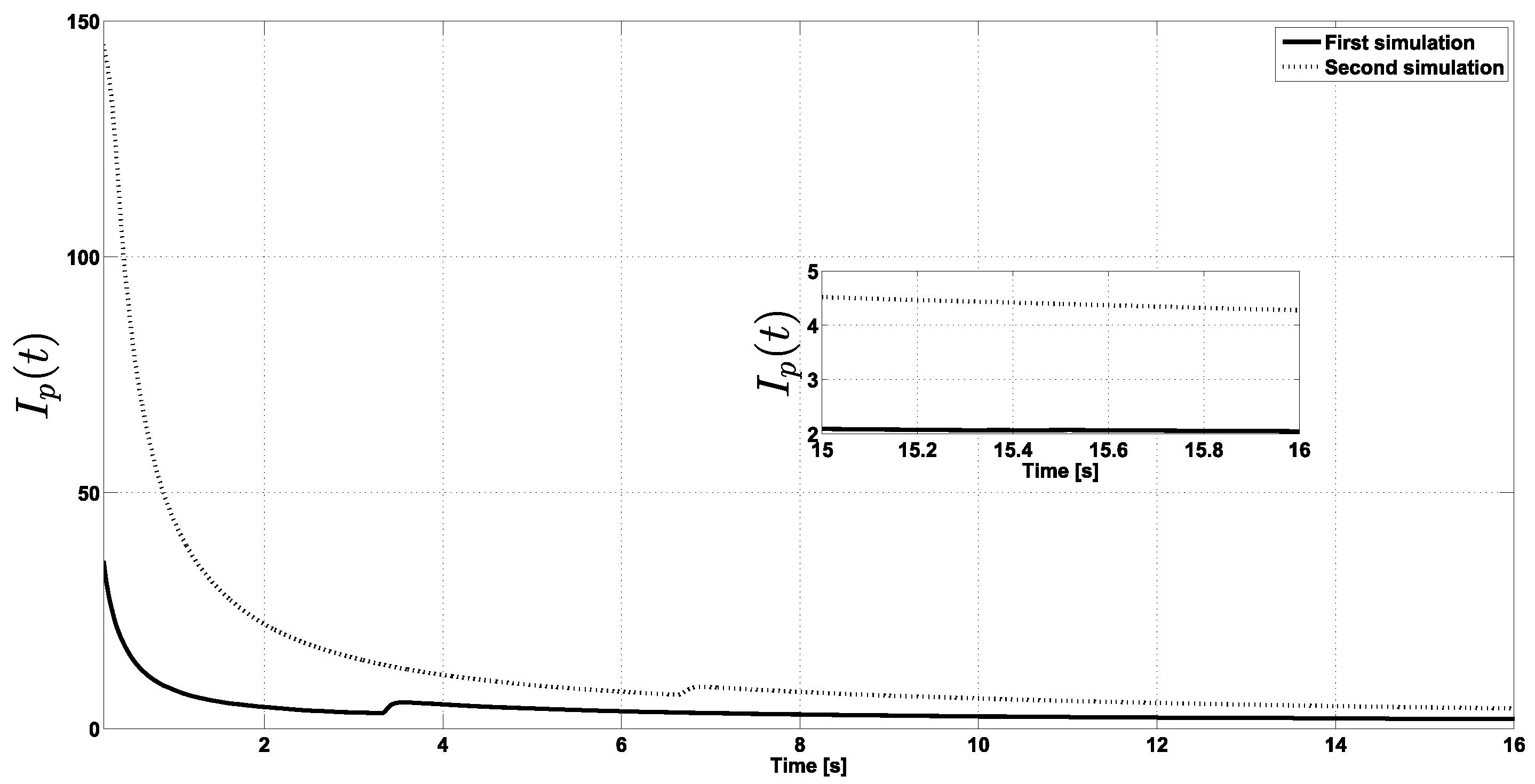
4. Numerical Simulations
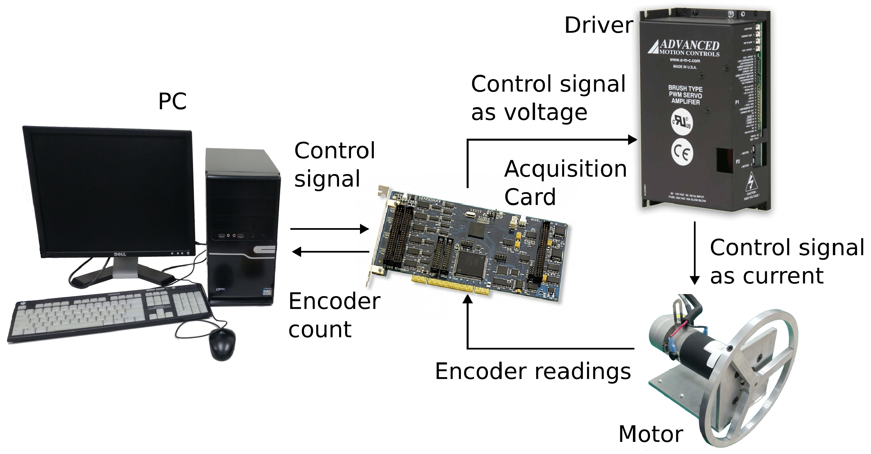
To test the effectiveness of the proposed observer scheme, two numerical experiments are designed using the rotating machine parameters taken from [1]. For both experiments, the following set-up is considered: J = 0.0011 kgm2 and k = 0.0009 kgm2/s.
First simulation. The task consists of recovering the non-available angular velocity w and estimating the unknown load torque τ L , where the random perturbations of the output signals ξ 11 and ξ 12 are uniformly distributed in the interval [ 0.05 , 0.05 ] . Similarly, the perturbation ζ that affects the mechanical model is a random signal uniformly distributed in the interval [ 0.05 , 0.05 ] . The load torque and its abrupt change are set as follows:
τ L = 0.25 if 0 < t 2 t * 02.5 if t * < t < 2 t * .
where t * = 3.3166 s. The observer uses the following gain matrices (where I 4 is a fourth-order identity matrix):
R = I 4 ; Q = 10 I 4
The suitable input is defined as
τ = J ( s i n ( . 25 t ) L + τ ^ L ) ,
where L = 30.15 . Figure 1 shows the outcome of this experiment. In the first plot of Figure 1, the actual angular velocity w and its estimation w ^ are shown. In this plot, it can be seen that w ^ overlaps w after 0.2 s until t * . In t * , the abrupt value change of τ L is introduced, as defined in (16). Consequently, information is lost and w ^ stops overlapping w during 0.25 s. Note that the SDRE observer in (12) and (14) can recover the estimated angular velocity w ^ in a very short period. This demonstrates, on the one hand, the observer’s efficiency and on the other, its robustness, as it can estimate the angular velocity even in the presence of random disturbances. In other words, the observer behaves as an effective filter. Note that the estimation w ^ is very close to w, even when the angular acceleration is noisily perturbed. This means that the estimation error is small, as the gain matrix Q is fixed to be sufficiently large. Additionally, the noise effect over w can be observed, contrary to the filtered signal w ^ , because the observer acts as a Kalman filter. To complement this, the second plot shows the behavior of τ L and its estimation τ ^ L . It can be seen that τ ^ L converges around τ L after 0.25 s, then, at 3.31 s the value of τ L abruptly changes, and the observer can reconstruct it after 0.25 s. As in the case of w, the observer very quickly estimates the new value of τ because, as already mentioned, the matrix Q is set to be sufficiently large. It should be remembered that the noise acts over the angular acceleration and the load torque, as can be seen in the τ ^ L behavior.
Second simulation. Now, the control task lies in having the rotary motor track the sinusoidal reference trajectory
w r ( t ) = L 2 sin ( w i t ) ,
where w i = 8 π / 400 . To make the task more challenging and test the SDRE observer’s performance and robustness, we introduce an abrupt change in the previously fixed load torque value according to the following rule:
τ L = 0.25 if 0 < t 2 t * 02.5 if 2 t * < t < 4 t * .
To carry out the control task, the following feedback is considered:
τ = J 2 ( w ^ w r ) + w . r + τ ^ L ,
where w ^ and τ ^ L are obtained according to the proposed observer. The setup and the random perturbations are considered as in the first experiment. Finally, the observer’s initial condition is set at the origin, and the motor initial condition is ( θ ( 0 ) = 1.5 rad, w ( 0 ) = 2 rad/s). Figure 2 shows the outcome of this simulation. In this figure, it can be seen in the first plot that after 0.3 s signals w, w r , and w ^ overlap, while in the second plot, it can be seen that τ L ^ is reconstructed after 0.3 s. Then, after 6.5 s, the abrupt change in the τ L is introduced. Again, after 0.5 s, signals w, w r , and w ^ overlap, and τ L is reconstructed. If both plots are examined carefully, the undesirable uniformly and bounded noise effect can be seen, even in the presence of this perturbation and the abrupt change in the value of τ L , the controller can fulfill the task. The observer continues reconstructing both estimations, w ^ and τ L ^ , reaching a steady state. This behavior shows that the controller and the observer are robust.
To provide an idea of how much the estimations of w ^ and τ ^ L deviate from the actual values, the performance indexes of the first and second simulations can be computed using the following formula:
I p ( t ) = 1 t 0 t ( w ^ ( s ) w ( s ) ) 2 + ( τ ^ L ( s ) τ L ( s ) ) 2 d s .
Figure 3 shows the obtained performance indexes of both simulations. Note that they have similar performances. Because the second simulation is a more complex task, its performance index is worse than that of the first simulation. At 3.31 s and 6.62 s, a performance loss in both simulations resulting from the abrupt load torque changes can be identified. However, the fast observer response overcomes the information loss, and the performance indexes return to their previous trend. In the image zoom, it can be seen that both performance indices converge to a steady state.

5. Experiments

Real-time experiments were conducted to test the observer’s performance in a practical setting. The experimental platform, shown in Figure 4, consisted of a PITTMAN ID23004 brushed DC motor driven by an Advanced Motion Controls driver model 16A20AC. The angular position of the motor was sensed by a US Digital quadrature encoder HB6M-2500-250-IE-D-H with a resolution of 10,000 pulses per revolution. A desktop computer running Windows XP controlled the drivers and received the encoder’s readings via a Sensory 626 data acquisition board. The control algorithm was implemented in MATLAB/Simulink R2007a using the real-time desktop kernel with a sampling period of 1 ms. The physical parameters of the motor were J = 0.00166 kgm 2 and k = 0.0001 kgm 2 /s.
Due to software and hardware limitations, solving the Riccati Equation (14) in each sampling is impossible. To overcome this issue, matrix L was calculated offline for some range of variables w and θ . For w, a range from −10 to 10 [rad/s] was used, while for θ the range was from 0 to 2 π . The range for θ was selected in this way because in matrix A e , the only non-constant term in (14), θ , is the argument of trigonometric functions. This means that with the selected range, all the possible values for these functions are included, making it unnecessary to include values of θ outside the used range. The gain matrix used for experiments was
R = I 4 ; Q = 10 I 4
In the experiment test, the angular velocity w was calculated by applying the filter presented in [50] to the readings of the motor encoder:
w ( k T ) = Q 2 ( z 1 ) Q 1 ( z 1 ) ( 1 z 1 ) ( p 2 + 1 ) ( p 1 + 1 ) T θ ( k T ) ,
where k is the time index, T is the sampling period Q 1 ( z 1 ) = 1 + z 1 + z 2 + + z p 1 , and Q 2 ( z 1 ) = 1 + z 1 + z 2 + + z p 2 . For the experiments presented below, p 1 and p 2 are selected as p 1 = p 2 = 4 .
First experiment. In this test, the task is to track the desired velocity defined as w r = sin ( 2.5 t ) + 3 using the control law (19) while a constant load torque of −0.3 Nm is applied. The results depicted in Figure 5 show that the estimation of the angular velocity converges in approximately 0.3 s, while the load torque estimation converges after 0.5 s. Note that although the torque estimation does not reach the value of 0.3 Nm, a satisfactory result is obtained for the angular velocity estimation.
Second experiment. In this test the desired velocity is defined as
w r ( t ) = w 0 + w f w 0 2 ( 1 + tanh ( t T ) ) ,
with w 0 = 0 , w f = 5 , and T = 0 , and the feedback controller provided in (19) is considered. The load torque is designed to change over time and is provided by
τ L = 0.3 , 0 t < 5 ; 0.2 , 5 t < 10 ; 0.3 , 10 t 15 .
As in the first experiment, it takes approximately 0.3 and 0.5 s for w ^ and τ ^ L to converge, respectively, at the beginning of the test and after each change in the load toque. These results are shown in Figure 6. Note that, as in the previous case, the torque estimation does not reach exactly the values provided in (20), although this does not prevent a satisfactory result with respect to speed estimation.
The index performance for both real-time experiments is shown in Figure 7, where it can be seen that both indexes tend to have a constant value as time progresses.
The steady-state errors of the torque load estimation observed in both experiments can be attributed to friction phenomena that were not considered in the design of the observer. For the first experiment, the variable error might be due to the Stribeck effect, which could explain the decrease in the error when the speed increases. In the second experiment, the almost constant error in τ ^ L can be attributed to the Coulomb friction.

6. Conclusions

This document focuses on designing a nonlinear observer for a rotating machine with a motor shaft and measurable outputs that are perturbed. As is well known, sensorless control of a rotating machine requires speed estimation. However, using speed encoders adds cost and reduces reliability, while the traditional methods for estimating speed, including approximate derivatives and numerical differentiation, can increase noise. The proposed solution avoids the need for these speeds and load torque estimation methods. To measure the angular position and load torque, the linear machine model is rewritten as a nonlinear system, allowing the non-available angular velocity and the unknown constant load torque to be estimated. To design the observer, the algebraic state-dependent Riccati equation is used to robustly estimate the angular velocity and load torque. The traditional Lyapunov method allows the development of the convergence analysis, guaranteeing estimation error convergence to a “ κ zone.” To assess the performance and validate the actual application of the proposed observer scheme, two numerical simulations were developed and two real-time experiments were conducted, obtaining satisfactory and convincing results in all cases.
A sine reference signal is established in the first numerical simulation and a constant load torque is assumed. In the second numerical simulation, a smooth step is considered; in this case, abrupt changes in the load torque at different times are introduced. Random perturbations uniformly distributed in certain magnitude intervals are added in both simulations. On the other hand, the two real-time experiments tracked the desired velocities, one with constant load torque and the other with a load torque that changes over time.

Author Contributions

Conceptualization, C.A.-I., M.A.J.-L., I.G.-E., J.M.-V., B.S., M.S.S.-C. and J.d.J.R.; Data curation, B.S. and M.S.S.-C.; Formal analysis, C.A.-I., M.A.J.-L., I.G.-E., J.M.-V., B.S., M.S.S.-C. and J.d.J.R.; Investigation, C.A.-I., M.A.J.-L., I.G.-E., J.M.-V., B.S., M.S.S.-C. and J.d.J.R.; Methodology, C.A.-I., M.A.J.-L., I.G.-E., J.M.-V., B.S., M.S.S.-C. and J.d.J.R.; Project administration, B.S. and M.S.S.-C.; Validation, I.G.-E., B.S. and M.S.S.-C.; Writing—original draft, C.A.-I., M.A.J.-L., I.G.-E., J.M.-V., B.S., M.S.S.-C. and J.d.J.R.; Writing— review and editing, C.A.-I., M.A.J.-L., I.G.-E., J.M.-V., B.S., M.S.S.-C. and J.d.J.R. All authors have read and agreed to the published version of the manuscript.

Funding

This study was financed in part by Instituto Politecnico Nacional of Mexico under research grants 20220436, 20220617, 20221667, and 20222110, by CONACyT Project A1-S-24762, México, Proyecto Apoyado por el Fondo Sectorial de Investigación para la Educación, and in part by CINVESTAV.

Institutional Review Board Statement

Not applicable.

Informed Consent Statement

Not applicable.

Data Availability Statement

Not applicable.

Acknowledgments

Carlos Aguilar-Ibanez, Javier Moreno-Valenzuela, Isaac Gandarilla-Esparza, Miguel S. Suarez-Castanon and Jose Rubio want to express their gratitude to the Instituto Politecnico Nacional. Manuel Jimenez-Lizarraga wants to express his gratitude to the Universidad Autonoma de Nuevo Leon, and Belem Saldivar wants to express her gratitude to CINVESTAV.

Conflicts of Interest

The authors declare no conflict of interest.

Appendix A

Proof that the system is locally observable, that is, the rank of matrix O defined in Equation (13) is equal to 4 for all w 0 .
Substituting the values of A e x and C provided in (11) and (8) into the relation (13) yields
det C CA e = 0 .
However,
Δ 2 = det C CA e 2 = det 1 0 0 0 0 1 0 0 z 1 2 4 0 k y 2 2 J y 1 z 1 4 y 2 2 0 z 1 2 4 k y 1 2 J y 2 z 1 4 y 1 2 = 1 8 y 1 2 + y 2 2 z 1 = z 1 8 .
Indeed, from the facts that y 1 2 + y 2 2 = sin 2 θ + cos 2 θ = 1 and z 1 = w , we have Δ 2 = w / 8 . The latter means that the rank of O is equal to 4 as long as w 0 .
Note that if the pair { A e x , C } is locally observable, the Riccati equation can always be solved, that is, Assumption 3 always holds, at least locally.
Proof that the matrix A e is Lipschitz.
Define the vectors
x = [ y 1 , y 2 , z 1 , z 2 ] T ; x = [ y 1 , y 2 , z 1 , z 2 ] T ,
then, according to Definition (11), we have
A e ( x + x ) A e ( x ) = 0 z 1 2 y 2 2 0 z 1 2 0 y 1 2 0 0 0 0 0 0 0 0 0 L f x .

References

  1. Shah, D.; Ortega, R.; Astolfi, A. Speed and load torque observer for rotating machines. In Proceedings of the 48h IEEE Conference on Decision and Control (CDC) Held Jointly with 2009 28th Chinese Control Conference, Shanghai, China, 16–18 December 2009; pp. 6143–6148. [Google Scholar]
  2. Chalanga, A.; Kamal, S.; Fridman, L.; Bandyopadhyay, B.; Moreno, J. How to implement Super-Twisting Controller based on sliding mode observer? In Proceedings of the 2014 13th International Workshop on Variable Structure Systems (VSS), Nantes, France, 29 June–2 July 2014; pp. 1–6. [Google Scholar] [CrossRef]
  3. Naghshtabrizi, P.; Hespanha, J. Designing an observer-based controller for a network control system. In Proceedings of the 44th IEEE Conference on Decision and Control, Seville, Spain, 12–15 December 2005; pp. 848–853. [Google Scholar] [CrossRef]
  4. Boulkroune, A.; Tadjine, M.; M’Saad, M.; Farza, M. How to design a fuzzy adaptive controller based on observers for uncertain affine nonlinear systems. Fuzzy Sets Syst. 2008, 159, 926–948. [Google Scholar] [CrossRef]
  5. Ley-Rosas, J.J.; González-Jiménez, L.E.; Loukianov, A.G.; Ruiz-Duarte, J.E. Observer based sliding mode controller for vehicles with roll dynamics. J. Frankl. Inst. 2019, 356, 2559–2581. [Google Scholar] [CrossRef]
  6. Has, Z.; Muslim, A.H.; Mardiyah, N.A. Adaptive-fuzzy-PID controller based disturbance observer for DC motor speed control. In Proceedings of the 2017 4th International Conference on Electrical Engineering, Computer Science and Informatics (EECSI), Yogyakarta, Indonesia, 19–21 September 2017; pp. 1–6. [Google Scholar] [CrossRef]
  7. Ertürk, A.T.; Karabay., S.; Baynal, S.K.; Korkut, T. Vibration Noise Harshness of a Light Truck Driveshaft, Analysis and Improvement with Six Sigma Approach. Acta Phys. Pol. 2017, 131, 477–480. [Google Scholar] [CrossRef]
  8. DeSmidt, H.; Wang, K.; Smith, E. Coupled Torsion-Lateral Stability of a Shaft-Disk System Driven Through a Universal Joint. J. Appl. Mech. 2002, 69, 261–273. [Google Scholar] [CrossRef]
  9. Linares-Flores, J.; Sira-Ramírez, H.; Yescas-Mendoza, E.; Vásquez-Sanjuan, J. A comparison between the algebraic and the reduced order observer approaches for on-line load torque estimation in a unit power factor rectifier-DC motor system. Asian J. Control 2012, 14, 45–57. [Google Scholar] [CrossRef]
  10. Li, B.; Goodarzi, A.; Khajepour, A.; Chen, S.k.; Litkouhi, B. An optimal torque distribution control strategy for four-independent wheel drive electric vehicles. Veh. Syst. Dyn. 2015, 53, 1172–1189. [Google Scholar] [CrossRef]
  11. Archela, A.; Toginho, D.G.; de Melo, L.F. Torque control of a DC motor with a state space estimator and Kalman filter for vehicle traction. In Proceedings of the 2018 13th IEEE International Conference on Industry Applications (INDUSCON), São Paulo, Brazil, 11–14 November 2018; pp. 763–769. [Google Scholar]
  12. Lian, C.; Xiao, F.; Gao, S.; Liu, J. Load torque and moment of inertia identification for permanent magnet synchronous motor drives based on sliding mode observer. IEEE Trans. Power Electron. 2018, 34, 5675–5683. [Google Scholar] [CrossRef]
  13. Archela, A.; Toginho, D.G.; de Melo, L.F. Torque Control of a DC Motor with a State Space Estimator and Kalman Filter Applied in Electrical Vehicles. In Applied Electromechanical Devices and Machines for Electric Mobility Solutions; IntechOpen: Rijeka, Croatia, 2019. [Google Scholar]
  14. Kumar, S.G.; Thilagar, S.H. Development of Load Torque Estimation and Passivity Based Control for DC Motor Drive Systems with Reduced Sensor Count. Emerg. Issues Sci. Technol. 2020, 3, 1–25. [Google Scholar]
  15. Srinivasan, G.K.; Srinivasan, H.T.; Rivera, M. Low-cost implementation of passivity-based control and estimation of load torque for a luo converter with dynamic load. Electronics 2020, 9, 1914. [Google Scholar] [CrossRef]
  16. Marino, R.; Tomei, P.; Verrelli, C. Adaptive control for speed-sensorless induction motors with uncertain load torque and rotor resistance. Int. J. Adapt. Control Signal Process. 2005, 19, 661–685. [Google Scholar] [CrossRef]
  17. Buja, G.S.; Menis, R.; Valla, M.I. Disturbance torque estimation in a sensorless DC drive. IEEE Trans. Ind. Electron. 1995, 42, 351–357. [Google Scholar] [CrossRef]
  18. Fabbri, S.; Nienhaus, M.; Grasso, E. Robust Load-Torque Estimation for DC Motor without Torque Sensor. In Proceedings of the 2019 AEIT International Annual Conference (AEIT), Florence, Italy, 18–20 September 2019; pp. 1–6. [Google Scholar]
  19. Kumar, S.G.; Thilagar, S.H. Sensorless load torque estimation and passivity based control of Buck converter fed DC motor. Sci. World J. 2015, 2015, 132843. [Google Scholar] [CrossRef] [PubMed] [Green Version]
  20. Mandriota, R.; Fabbri, S.; Nienhaus, M.; Grasso, E. Sensorless Pedalling Torque Estimation Based on Motor Load Torque Observation for Electrically Assisted Bicycles. Actuators 2021, 10, 88. [Google Scholar] [CrossRef]
  21. Holtz, J. Sensorless control of induction motor drives. Proc. IEEE 2002, 90, 1359–1394. [Google Scholar] [CrossRef] [Green Version]
  22. Loria, A.; Espinosa-Pérez, G.; Chumacero, E. A novel PID-based control approach for switched-reluctance motors. In Proceedings of the 2012 IEEE 51st IEEE Conference on Decision and Control (CDC), Maui, HI, USA, 10–13 December 2012; pp. 7626–7631. [Google Scholar]
  23. Ortega, R.; Praly, L.; Astolfi, A.; Lee, J.; Nam, K. Estimation of rotor position and speed of permanent magnet synchronous motors with guaranteed stability. IEEE Trans. Control Syst. Technol. 2010, 19, 601–614. [Google Scholar] [CrossRef]
  24. Bullinger, E.; Allgower, F. An adaptive high-gain observer for nonlinear systems. In Proceedings of the 36th IEEE Conference on Decision and Control, San Diego, CA, USA, 10 December 1997; Volume 5, pp. 4348–4353. [Google Scholar]
  25. Guerra, R.M.; Poznyak, A.; De Leon, V.D. Robustness property of high-gain observers for closed-loop nonlinear systems: Theoretical study and robotics control application. Int. J. Syst. Sci. 2000, 31, 1519–1529. [Google Scholar] [CrossRef]
  26. Nicosia, S.; Tomei, P.; Tornambé, A. A nonlinear observer for elastic robots. IEEE J. Robot. Autom. 1988, 4, 45–52. [Google Scholar] [CrossRef]
  27. Walcott, B.; Zak, S. State observation of nonlinear uncertain dynamical systems. IEEE Trans. Autom. Control 1987, 32, 166–170. [Google Scholar] [CrossRef]
  28. Ciccarella, G.; Dalla Mora, M.; Germani, A. A Luenberger-like observer for nonlinear systems. Int. J. Control 1993, 57, 537–556. [Google Scholar] [CrossRef]
  29. Gauthier, J.; Bornard, G. Observability for any u (t) of a class of nonlinear systems. IEEE Trans. Autom. Control 1981, 26, 922–926. [Google Scholar] [CrossRef]
  30. Poznyak, A.; Martinez-Guerra, R.; Osorio-Cordero, A. Robust high-gain observer for nonlinear closed-loop stochastic systems. Math. Probl. Eng. 2000, 6, 31–60. [Google Scholar] [CrossRef]
  31. Zeitz, M. The extended Luenberger observer for nonlinear systems. Syst. Control Lett. 1987, 9, 149–156. [Google Scholar] [CrossRef]
  32. Linares-Flores, J.; Barahona-Avalos, J.L.; Sira-Ramirez, H.; Contreras-Ordaz, M.A. Robust passivity-based control of a buck–boost-converter/DC-motor system: An active disturbance rejection approach. IEEE Trans. Ind. Appl. 2012, 48, 2362–2371. [Google Scholar] [CrossRef]
  33. Sira-Ramírez, H.; González-Montañez, F.; Cortés-Romero, J.A.; Luviano-Juárez, A. A robust linear field-oriented voltage control for the induction motor: Experimental results. IEEE Trans. Ind. Electron. 2012, 60, 3025–3033. [Google Scholar] [CrossRef]
  34. Linares-Flores, J.; Sira-Ramirez, H.; Cuevas-Lopez, E.F.; Contreras-Ordaz, M.A. Sensorless passivity based control of a DC motor via a solar powered Sepic converter-full bridge combination. J. Power Electron. 2011, 11, 743–750. [Google Scholar] [CrossRef] [Green Version]
  35. Davila, J.; Fridman, L.; Levant, A. Second-order sliding-mode observer for mechanical systems. IEEE Trans. Autom. Control 2005, 50, 1785–1789. [Google Scholar] [CrossRef]
  36. Edwards, C.; Spurgeon, S. Sliding Mode Control: Theory and Applications; CRC Press: Boca Raton, FL, USA, 1998. [Google Scholar]
  37. Shtessel, Y.B.; Poznyak, A.S. Parameter identification of affine time varying systems using traditional and high order sliding modes. In Proceedings of the 2005 American Control Conference, Portland, OR, USA, 8–10 June 2005; pp. 2433–2438. [Google Scholar]
  38. Shtessel, Y.; Edwards, C.; Fridman, L.; Levant, A. Sliding Mode Control and Observation; Springer: New York, NY, USA, 2014; Volume 10. [Google Scholar]
  39. Yaz, E.; Azemi, A. Robust/adaptive observers for systems having uncertain functions with unknown bounds. In Proceedings of the 1994 American Control Conference—ACC’94, Baltimore, MD, USA, 29 June–1 July 1994; Volume 1, pp. 73–74. [Google Scholar]
  40. Zhu, R.; Chai, T.; Shao, C. Robust nonlinear adaptive observer design using dynamic recurrent neural networks. In Proceedings of the 1997 American Control Conference (Cat. No. 97CH36041), Albuquerque, NM, USA, 6 June 1997; Volume 2, pp. 1096–1100. [Google Scholar]
  41. Mracek, C.P.; Cloutier, J.R. Control designs for the nonlinear benchmark problem via the state-dependent Riccati equation method. Int. J. Robust Nonlinear Control 1998, 8, 401–433. [Google Scholar] [CrossRef]
  42. Liu, J.; Wang, L.; Shi, Z. Dynamic modelling of the defect extension and appearance in a cylindrical roller bearing. Mech. Syst. Signal Process. 2022, 173, 109040. [Google Scholar] [CrossRef]
  43. Liu, J.; Xu, Z. A simulation investigation of lubricating characteristics for a cylindrical roller bearing of a high-power gearbox. Tribol. Int. 2022, 167, 107373. [Google Scholar] [CrossRef]
  44. Karagiannis, D.; Astolfi, A. Observer design for a class of nonlinear systems using dynamic scaling with application to adaptive control. In Proceedings of the 2008 47th IEEE Conference on Decision and Control, Cancun, Mexico, 9–11 December 2008; pp. 2314–2319. [Google Scholar]
  45. Bobtsov, A.A.; Pyrkin, A.A.; Ortega, R.; Vukosavic, S.N.; Stankovic, A.M.; Panteley, E.V. A robust globally convergent position observer for the permanent magnet synchronous motor. Automatica 2015, 61, 47–54. [Google Scholar] [CrossRef]
  46. Çimen, T. State-dependent Riccati equation (SDRE) control: A survey. IFAC Proc. Vol. 2008, 41, 3761–3775. [Google Scholar] [CrossRef] [Green Version]
  47. Beikzadeh, H.; Taghirad, H.D. Exponential nonlinear observer based on the differential state-dependent Riccati equation. Int. J. Autom. Comput. 2012, 9, 358–368. [Google Scholar] [CrossRef]
  48. Çimen, T. Systematic and effective design of nonlinear feedback controllers via the state-dependent Riccati equation (SDRE) method. Annu. Rev. Control 2010, 34, 32–51. [Google Scholar] [CrossRef]
  49. Haessig, D.A.; Friedland, B. State dependent differential Riccati equation for nonlinear estimation and control. IFAC Proc. Vol. 2002, 35, 405–410. [Google Scholar] [CrossRef] [Green Version]
  50. Moreno-Valenzuela, J.; Campa, R.; Santibáñez, V. Model-based control of a class of voltage-driven robot manipulators with non-passive dynamics. Comput. Electr. Eng. 2013, 39, 2086–2099. [Google Scholar] [CrossRef]
Figure 1. Open-loop estimation of w and τ L with u fixed as in (19).
Machines 10 01009 g001
Figure 2. Variable and parameter estimations for tracking of a trajectory implemented as a smooth step.
Machines 10 01009 g002
Figure 3. Performance index of the first and second experiments.
Machines 10 01009 g003
Figure 4. Experimental platform used for real-time tests.
Machines 10 01009 g004
Figure 5. Variable and parameter estimations for the case λ = 1 and matrix Q = 10 I 4 .
Machines 10 01009 g005
Figure 6. Variable and parameter estimations for the tracking of a trajectory implemented as a smooth step.
Machines 10 01009 g006
Figure 7. Performance index of first and second experiments.
Machines 10 01009 g007
Publisher’s Note: MDPI stays neutral with regard to jurisdictional claims in published maps and institutional affiliations.

