A Novel Optimistic Local Path Planner: Agoraphilic Navigation Algorithm in Dynamic Environment

Abstract

This paper presents a novel local path planning algorithm developed based on the new free space attraction (Agoraphilic) concept. The proposed algorithm is capable of navigating robots in unknown static, as well as dynamically cluttered environments. Unlike the other navigation algorithms, the proposed algorithm takes the optimistic approach of the navigation problem. It does not look for problems to avoid, but rather for solutions to follow. This human-like decision-making behaviour distinguishes the new algorithm from all the other navigation algorithms. Furthermore, the new algorithm utilises newly developed tracking and prediction algorithms, to safely navigate mobile robots. This is further supported by a fuzzy logic controller designed to efficiently account for the inherent high uncertainties in the robot’s operational environment at a reduced computational cost. This paper also includes physical experimental results combined with bench-marking against other recent methods. The reported results verify the algorithm’s successful advantages in navigating robots in both static and dynamic environments.

1. Introduction

Mobile robots have become important machines for many sectors in today’s world, including mining [1], space [2], surveillance [3], military applications [4], hospital work [5], agriculture [6], and many others [7]. Navigation is an important element in mobile robots’ functionality. Unlike autonomous vehicles, the mobile robot’s operational environment, in most cases, is not specifically engineered for the robot. Therefore, from a navigational perspective, the robot must be able to operate in an unpredictable dynamic environment. This environmental complexity requires the robot to make navigational decisions in real-time. Therefore, an efficient autonomous navigation system should be characterised by the ability to navigate robots in unknown dynamic environments using real-time decision-making algorithms.

The literature describes a number of path planning methods [8] such as the genetic algorithm (GA) [9], artificial neural networks (ANNs) [10], deep reinforcement learning (DRL) [11], fuzzy logic (FL) [12], gradient-based planners (GBP) [13], bio-inspired path planning methods [14], roadmaps [15], cell decomposition [16], and artificial potential field (APF) [17].

Among these techniques, the APF-based method has been widely used because of its simplicity and adaptability. However, there are some well-documented problems inherent to APF-based methods [17], with multiple algorithms developed to address and overcome these drawbacks [18,19,20,21,22,23]. Among those attempts is the original Agoraphilic navigation algorithm [24]. Its uniqueness stems from the fact that it offers a single integrated solution to all the essential difficulties of the APF-based methods, rather than providing individual solutions for each problematic element.

The original Agoraphilic algorithm addressed the principal issues of the APF-based methods by introducing a new, free space attraction (Agoraphilic) concept. The main problem with the original Agoraphilic algorithm is that it is restricted to static environments. This presents significant problems to most real-world applications for mobile robots, as they frequently operate in unknown dynamic environments. This limitation of the original Agoraphilic algorithm provided the primary motivation to develop the proposed algorithm: the Agoraphilic navigation algorithm in dynamic environments (ANADE).

Dynamic environments are characterised by high levels of uncertainty, thereby presenting significant challenges to navigational algorithms [16]. Navigational techniques based on artificial intelligence (AI) are frequently used to address this problem [25]. Among these, fuzzy logic is commonly used to overcome uncertainties at a low computational cost. Most alternative existing navigation algorithms fail to use the speed and the moving direction of dynamic obstacles as an input for decision-making. This is due to the difficulty of estimating the velocity vectors of moving obstacles [26,27]. Consequently, most existing navigation algorithms are unable to navigate in uncertain dynamic environments, leading in turn to sub-optimal performance or system failure in complex situations [26]. The novel ANADE uses a fuzzy-logic-based controller, a tracking algorithm, and a dynamic object pathway prediction module to overcome these limitations.

The ANADE does not identify obstacles (problems) to avoid, but rather follows existing and predicted free space corridors (solutions) towards the goal. The algorithm uses only one attractive force, created by the available current and predicted future growing free space within the robot’s environment. This attractive force pulls the robot through free space passages towards the goal. The algorithm was tested by simulations, as well as by real-world experiments using the TurtleBot3 robot platform.

Section 2 of this paper discusses the development of the ANADE. The development of the experimental configuration and real-world experimental results are presented in Section 3. Section 4 provides a discussion of our findings and concluding remarks.

2. Development of the Agoraphilic Navigation Algorithm in Dynamic Environment

The ANADE consists of eight main modules:

• Sensory data processing (SDP) module;
• Obstacle tracking (OT) module;
• Dynamic obstacles’ position prediction (DOPP) module;
• Current and future free space histogram (FSH) generation module;
• Free space force (FSF) generation module;
• Force-shaping module;
• Instantaneous driving Force component (F_c) generation module;
• Instantaneous driving force component weighting module.

The SDP module collects data from the sensors mounted on the robot (LiDAR, Real Sense camera, encoders, and associated equipment) and transforms all robot-centric data to a world reference frame (Global Positioning System). The OT module then generates two outputs, a current global map (CGM) and the states (position and velocity) of dynamic obstacles within the map using the globalised sensory data.

Subsequently, the algorithm is divided into two sections:

• F_c generation for the current global map (CGM)-CGM-F_c1;
• F_c generation for the future global maps (FGMs)-F_c2, F_c3, …, F_cN (prediction).

The F_c generation for the CGM (F_c1) section of the algorithm uses the current environment of the robot (the CGM) and generates the component force (F_c1) based on the current surroundings of the robot. In this process, the CGM becomes the input for the FSH generation module. The created FSH is then transformed to a set of free space forces (FSFs) by the free space force generation module. Subsequently, the force-shaping module regulates the FSFs such that the robot will move towards the goal. Finally, the F_c generation module generates the final driving force component (F_c) for the CGM using the shaped FSFs.

The current states of moving obstacles are used as the input for the dynamic obstacles’ position prediction module. This returns N-1 future global maps, where N is the final prediction of the DOPP module. Each FGM is fed into the FSH generation module. The created FSH is then transformed to a set of predictive FSFs by the FSF generation module. Subsequently, the force-shaping module shapes the FSFs such that the robot will move towards the goal. Finally, the F_c generation module generates the F_c for the corresponding future global map. This process occurs for each FGM.

Finally, all the instantaneous driving force components (F_c1, F_c2, …, F_cN) related to the current and future global maps are fed into the instantaneous driving force component weighting module. This module generates the final driving force, the robot’s actual driving force for the current iteration. This process repeats for each iteration.

The development of these sub-modules is discussed in the following subsections.

2.1. Sensory Data Processing Module

The SDP module takes sensory data as its input from the robot’s sensory system. The robot’s environment is captured using two sensory systems:

• A 360⁰ LiDAR sensor;
• A Real Sense camera.

The SDP module receives LiDAR data as a point cloud. This point cloud is generated with respect to the robot’s coordinate system. The red, green, and blue (RGB) data captured by the Real Sense camera and the point cloud are pre-processed by a separate system (further discussed in Section 3). This system runs an image processing algorithm and combines depth information to provide the locations of obstacles with respect to the robot’s axis system. All data received with respect to this system are converted to the world reference frame through Equation (1). This module takes ∼2.5% of the overall processing time.

$$\begin{array}{c}\hfill \left[\begin{array}{c}Xg\\ Yg\end{array}\right]=\left[\begin{array}{cc}cos\left(\theta \right)& -sin\left(\theta \right)\\ sin\left(\theta \right)& cos\left(\theta \right)\end{array}\right]\times \left[\begin{array}{c}Xr\\ Yr\end{array}\right]+\left[\begin{array}{c}Xrg\\ Yrg\end{array}\right]\end{array}$$

(1)

$\theta$	$\stackrel{\mathrm{def}}{=}$	orientation of the robot
$(Xg,Yg)$	$\stackrel{\mathrm{def}}{=}$	coordinates with respect to
		the world reference frame
$(Xr,Yr)$	$\stackrel{\mathrm{def}}{=}$	coordinates with respect to
		the robot’s axis system
$(Xrg,Yrg)$	$\stackrel{\mathrm{def}}{=}$	robot’s current position with
		respect to the world reference frame

2.2. Obstacle Tracking Module

The SDP module feeds obstacles’ positions to the obstacle tracking module. This module generates two outputs:

(1)

The current global map (CGM): This map represents the robot’s surrounding environment with respect to the global coordinate frame. The CGM consists of information about the current locations of static and moving obstacles.

(2)

The estimated states( position and velocity) of dynamic obstacles: The position and velocity of moving obstacles are given by the estimated states.

The proposed tracking module was developed using two sub-modules, a measurement module and a process module. A Kalman filter is used to combine the outputs of these two modules to estimate the states of moving obstacles. The Kalman-filter-based algorithm has been shown to be capable of tracking slow-moving objects successfully [28,29].

In the OT module, the kinematic model of moving obstacles is defined as follows (Equation (2)):

$$\begin{array}{ccc}\hfill \left[\begin{array}{c}{x}_k\\ y_k\\ {\dot{x}}_k\\ {\dot{y}}_k\end{array}\right]& =& \left[\begin{array}{cccc}1& 0& dt& 0\\ 0& 1& 0& dt\\ 0& 0& 1& 0\\ 0& 0& 0& 1\end{array}\right]\left[\begin{array}{c}{x}_{k-1}\\ y_{k-1}\\ {\dot{x}}_{k-1}\\ {\dot{y}}_{k-1}\end{array}\right]+\hfill \\ & & \left[\begin{array}{c}{a}_x\times \frac{d{t}^2}{2}\\ a_y\times \frac{d{t}^2}{2}\\ a_x\times dt\\ a_y\times dt\end{array}\right]\begin{array}{c}u\left(t\right)\end{array}+\begin{array}{c}{w}_k\end{array}\hfill \end{array}$$

(2)

$$\begin{array}{ccc}\hfill \left[\begin{array}{c}{x}_k\\ y_k\end{array}\right]& =& \left[\begin{array}{cccc}1& 0& 0& 0\\ 0& 1& 0& 0\end{array}\right]+v_k\hfill \\ \hfill \end{array}$$

The prior estimation (state estimation based on the previous state estimation) and globalised sensory data (measurements (x_k,m, y_k,m)) are combined using the filter shown in Equation (3) to derive the optimal state estimations for each moving obstacle in each iteration.

$$\begin{array}{ccc}\hfill \left[\begin{array}{c}{x}_k\\ y_k\\ {\dot{x}}_k\\ {\dot{y}}_k\end{array}\right]& =& \left[\begin{array}{cccc}1& 0& dt& 0\\ 0& 1& 0& dt\\ 0& 0& 1& 0\\ 0& 0& 0& 1\end{array}\right]\left[\begin{array}{c}{x}_{k-1}\\ y_{k-1}\\ {\dot{x}}_{k-1}\\ {\dot{y}}_{k-1}\end{array}\right]+\hfill \\ & & \left[\begin{array}{c}{a}_x\times \frac{d{t}^2}{2}\\ a_y\times \frac{d{t}^2}{2}\\ a_x\times dt\\ a_y\times dt\end{array}\right]\begin{array}{c}u\left(t\right)\end{array}+k_k\{\left[\begin{array}{c}{x}_{k,m}\\ y_{k,m}\end{array}\right]-\hfill \\ & & {\left[\begin{array}{cc}1& 0\\ 0& 1\\ 0& 0\\ 0& 0\end{array}\right]}^T(\left[\begin{array}{cccc}1& 0& dt& 0\\ 0& 1& 0& dt\\ 0& 0& 1& 0\\ 0& 0& 0& 1\end{array}\right]\left[\begin{array}{c}{x}_{k-1}\\ y_{k-1}\\ {\dot{x}}_{k-1}\\ {\dot{y}}_{k-1}\end{array}\right]\hfill \\ & & +\left[\begin{array}{c}{a}_x\times \frac{d{t}^2}{2}\\ a_y\times \frac{d{t}^2}{2}\\ a_x\times dt\\ a_y\times dt\end{array}\right]\begin{array}{c}u\left(t\right)\end{array}\left)\right\}\hfill \end{array}$$

(3)

In this expression, k_k (Kalman gain) is found by using Equation (4):

$$\begin{array}{ccc}\hfill k_k& =& p_k{\left[\begin{array}{cc}1& 0\\ 0& 1\\ 0& 0\\ 0& 0\end{array}\right]}^T{\left({\left[\begin{array}{cc}1& 0\\ 0& 1\\ 0& 0\\ 0& 0\end{array}\right]}^T{p}_k\left[\begin{array}{cc}1& 0\\ 0& 1\\ 0& 0\\ 0& 0\end{array}\right]\right)}^{-1}\hfill \end{array}$$

(4)

where:

$$\begin{array}{ccc}\hfill p_k& =& \left[\begin{array}{cccc}1& 0& dt& 0\\ 0& 1& 0& dt\\ 0& 0& 1& 0\\ 0& 0& 0& 1\end{array}\right]p_{k-1}\left[\begin{array}{cccc}1& 0& 0& 0\\ 0& 1& 0& 0\\ dt& 0& 1& 0\\ 0& dt& 0& 1\end{array}\right]+Q\hfill \end{array}$$

At each iteration following the optimal state estimation of every moving obstacle, p_k is updated as shown in Equation (5).

$$\begin{array}{ccc}\hfill p_k& =& \left[\begin{array}{cccc}1& 0& 0& 0\\ 0& 1& 0& 0\\ 0& 0& 1& 0\\ 0& 0& 0& 1\end{array}\right]-k_k\left[\begin{array}{cccc}1& 0& dt& 0\\ 0& 1& 0& dt\\ dt& 0& 1& 0\\ 0& dt& 0& 1\end{array}\right]\times \hfill \\ & & p_{k-1}\left[\begin{array}{cccc}1& 0& dt& 0\\ 0& 1& 0& dt\\ dt& 0& 1& 0\\ 0& dt& 0& 1\end{array}\right]+Q\hfill \end{array}$$

(5)

where:

$v_k$	∼	N(0,R)
$w_k$	∼	N(0,Q)
p	$\stackrel{\mathrm{def}}{=}$	error covariance
$(x_k,y_k)$	$\stackrel{\mathrm{def}}{=}$	estimated position of
		the moving obstacle
$(x_{km},y_{km})$	$\stackrel{\mathrm{def}}{=}$	measured position of
		the moving obstacle
$(a_x,a_y)$	$\stackrel{\mathrm{def}}{=}$	acceleration of the
		moving obstacle

The OT module takes ∼11% of the overall processing time.

2.3. Dynamic Obstacle Position Prediction Module

The proposed algorithm identifies future growing or diminishing free spaces with the assistance of the DOPP module. The DOPP module estimates the future locations and velocities of dynamic obstacles in the robot’s environment.

The DOPP module uses globalised sensory data and information about the current locations and velocities of dynamic obstacles from the SDP and tracking modules as its primary inputs. The DOPP module then forecasts the robot’s anticipated environmental configuration for future iterations and develops FGMs based on this information. These FGMs are the outputs of the DOPP module (if the prediction is performed for t + n iterations, there will be n − 1 future global maps). As mentioned, the future locations and velocities of moving obstacles are predicted using the developed DOPP model, Equation (6). These predictions are updated at each iteration, and new predictions are made according to the updated state (location and velocity) data.

The future global map at iteration “N” is created by combining the positions of moving obstacles in the N^th iteration with the positions of static obstacles, both with respect to the robot’s future location, Equation (7). These future global maps are used for future FSH creation [30]. This module takes ∼5% of the overall processing time.

$$\begin{array}{c}\hfill \left[\begin{array}{c}x(t+n)\\ y(t+n)\\ dx(t+n)/dt\\ dy(t+n)/dt\end{array}\right]=\left[\begin{array}{cccc}1& 0& nT& 0\\ 0& 1& 0& nT\\ 0& 0& 1& 0\\ 0& 0& 0& 1\end{array}\right]\left[\begin{array}{c}x\left(t\right)\\ y\left(t\right)\\ \frac{dx\left(t\right)}{dt}\\ \frac{dy\left(t\right)}{dt}\end{array}\right]+\\ \hfill \left[\begin{array}{c}\frac{{\left(nT\right)}^2}{2}\\ \frac{{\left(nT\right)}^2}{2}\\ nT\\ nT\end{array}\right]\left[\begin{array}{c}\frac{d^{2}x\left(t\right)}{d{t}^2}\\ \frac{d^{2}y\left(t\right)}{d{t}^2}\\ \frac{d^{2}x\left(t\right)}{d{t}^2}\\ \frac{d^{2}y\left(t\right)}{d{t}^2}\end{array}\right]\end{array}$$

(6)

$$\begin{array}{c}\hfill \left[\begin{array}{c}x(k+1)\\ y(k+1)\\ \theta (k+1)\end{array}\right]=\left[\begin{array}{ccc}1& 0& 0\\ 0& 1& 0\\ 0& 0& 1\end{array}\right]\left[\begin{array}{c}{x}_k\\ y_k\\ {\theta }_k\end{array}\right]+\\ \hfill \left[\begin{array}{c}{\dot{x}}_k\\ {\dot{y}}_k\\ {\dot{\theta }}_k\end{array}\right]n\times T\end{array}$$

(7)

(x, y): the actual position coordinates.

$\theta$: orientation of the robot.

2.4. Free Space Histogram Generation Module

A robot-centric polar map is developed by the FSH generation module. Global maps are taken as the input of this module. The developed polar map indicates the free space around the robot of the input global map. Then, this polar map is transformed to a free space histogram. This transformation process is described below.

The global map is initially divided into K neighbouring sectors, themselves divided into cells. For all the occupied cells, a predetermined safety boundary (r) is applied. The closest occupied cell to the robot is identified. The sector distance (d_k) is the distance to the safety boundary corresponding to this closest cell. The FSH is then obtained based on the calculated sector distances. This module takes ∼35% of the overall processing time.

2.5. Free-Space Force Generation Module

The main input to the FSF generation module is an FSH. The FSF generation module generates force components using the information in the FSH. Generally, this force component is directly proportional to the normalised sector distance.

However, if the sector distance (d_k) is greater than the pre-determined d_max value, the force for the corresponding sector is taken as u_k [31]. This force component is known as the sector force (F_k). When an open space is bigger the corresponding F_k becomes larger. The output of the FSF generation module is a set of free space forces connected with each sector in the global map. This module takes ∼1.5% of the overall processing time.

2.6. Force-Shaping Module

This module takes a set of free space forces as its input. These free space forces need to be directed towards the goal. A weighting method is used to perform this task. The force-shaping module is considered to be one of the most important parts of the algorithm, as it has a direct influence on selecting the robot’s driving direction in the corresponding iteration. Furthermore, this module requires the highest processing power (∼42% of the overall processing time).

To perform this task, a numerical weighting system and a fuzzy logic controller are used.

2.6.1. Numerical Function

In this method, FSFs pointing towards the goal are allocated a higher weighting factor compared to FSFs pointing away from the goal. All the sector forces (F_k) are modified by a numerical force-shaping coefficient (${\delta }_N$). The numerical force-shaping coefficients are determined by Equation (8). The numerical force-shaping coefficient is set to its maximum value when the corresponding F_k points directly towards the goal.

$$\delta \left(\theta \right)=\left\{\begin{array}{cc}\frac{2}{\pi }\theta +1,\hfill & \mathrm{if}-\pi /2\le \theta \le 0;\hfill \\ \frac{-2}{\pi }\theta +1,\hfill & \mathrm{if}0\le \theta \le \pi /2;\hfill \\ \frac{2}{\pi }\theta -3,\hfill & \mathrm{if}3\pi /2\le \theta \le 2\pi ;\hfill \\ \frac{-2}{\pi }\theta -3,\hfill & \mathrm{if}-3\pi /2\le \theta \le 2\pi ;\hfill \\ 0,\hfill & \mathrm{otherwise}.\hfill \end{array}\right.$$

(8)

2.6.2. Fuzzy Logic Controller

The numerical weighting system quantifies the shaping factors by only considering the angle difference between the sector angle and robot-to-goal angle. In a cluttered dynamic environment, this single factor does not have sufficient spatial or temporal resolution. To perform more effectively, the system must consider other parameters such as the sector distances and speeds of moving obstacles. Further, having increased flexibility in shaping forces yields advantages in refined decision-making. Therefore, a fuzzy-logic-controller-based force-shaping module is also embedded in the force-shaping module. The rest of this sub-section discusses this controller.

A linguistic fuzzy model, known as the “Mandani Approach”, was used to develop the fuzzy logic controller. Its basic components are shown in Figure 1 and comprise four main modules:

• A fuzzification module;
• A fuzzy rule base;
• A fuzzy inference engine;
• A defuzzification module.

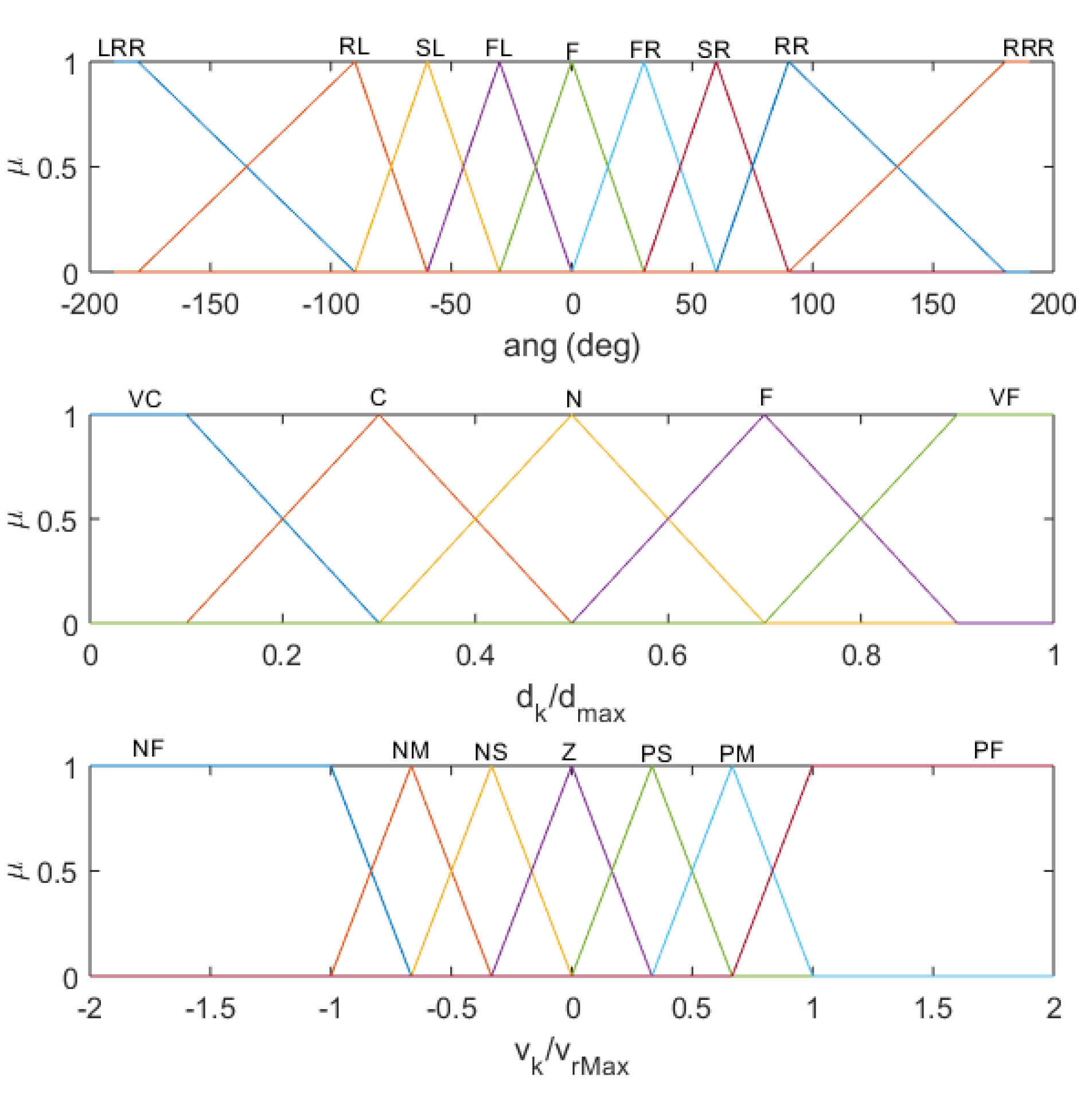
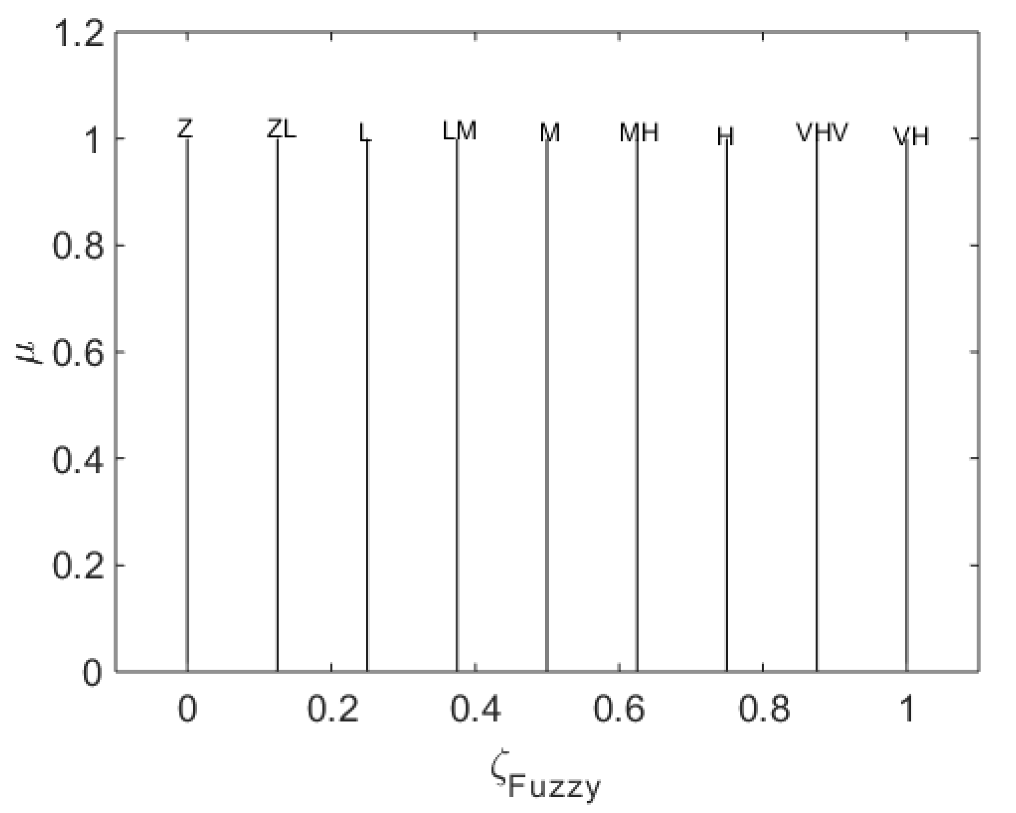
To develop the fuzzification module, four databases were designed. Three databases were used for the three inputs (${\theta }_{diff}$, d_k,n, and v_k,n) (Figure 2) and one for the output, the fuzzy shaping factor (${\delta }_f$) (Figure 3).

The three input databases were modelled using multiple fuzzy datasets. For all membership functions over a given universe of discourse, the membership function of a fuzzy set S, denoted by ${\mu }_s$, maps elements x ∈ X into a numerical value in the closed unit interval, for example:

${\mu }_s$ (x): → [0, 1]

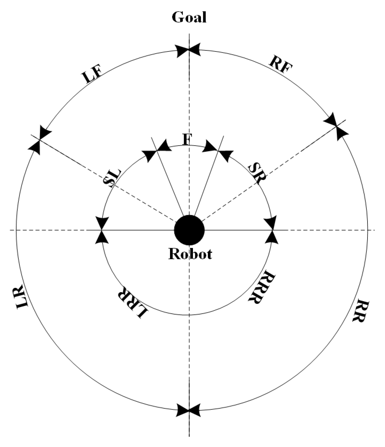
The database for the first input ${\theta }_{diff}$ consists of nine fuzzy membership functions derived from Equation (9). The corresponding linguistics are LRR: left rear rear, LR: left rear, SL: side left, LF: left front, F: front, RF: right front, SR: right side, RR: right rear, and RRR: right rear rear (Figure 4).

$$\begin{array}{c}\hfill {\mu }_{LRR}\left(\theta \right)=max\{min\left(\frac{-90-\theta }{90},1\right),0\}\\ \hfill {\mu }_{LR}\left(\theta \right)=max\{min\left(\frac{\theta +180}{90},\frac{-60-\theta }{30}\right),0\}\\ \hfill {\mu }_{SL}\left(\theta \right)=max\{min\left(\frac{\theta +90}{30},\frac{-30-\theta }{30}\right),0\}\\ \hfill {\mu }_{LF}\left(\theta \right)=max\{min\left(\frac{\theta +60}{30},\frac{-\theta }{30}\right),0\}\\ \hfill {\mu }_F\left(\theta \right)=max\{min\left(\frac{\theta +30}{30},\frac{30-\theta }{30}\right),0\}\\ \hfill {\mu }_{RF}\left(\theta \right)=max\{min\left(\frac{\theta }{30},\frac{60-\theta }{30}\right),0\}\\ \hfill {\mu }_{SR}\left(\theta \right)=max\{min\left(\frac{\theta -60}{30},\frac{180-\theta }{90}\right),0\}\\ \hfill {\mu }_{RR}\left(\theta \right)=max\{min\left(\frac{\theta -60}{30},\frac{180-\theta }{90}\right),0\}\\ \hfill {\mu }_{RRR}\left(\theta \right)=max\{min\left(\frac{\theta -90}{90},1\right),0\}\end{array}$$

(9)

where: $\theta \in$ {−180, 180}.

The database for the second input, the normalised sector distance (d_k,n), consists of five fuzzy membership functions, as shown in Equation (10). The corresponding linguistics are VC: very close, C: close, N: near, F: far, VF: very far.

$$\begin{array}{c}\hfill {\mu }_{VC}\left(d_{k,n}\right)=max\{min\left(\frac{-d_{k,n}-0.3}{0.2},1\right),0\}\\ \hfill {\mu }_C\left(d_{k,n}\right)=max\{min\left(\frac{d_{k,n}-0.1}{0.2},\frac{0.5-d_{k,n}}{0.2}\right),0\}\\ \hfill {\mu }_N\left(d_{k,n}\right)=max\{min\left(\frac{d_{k,n}-0.3}{0.2},\frac{0.7-d_{k,n}}{0.2}\right),0\}\\ \hfill {\mu }_F\left(d_{k,n}\right)=max\{min\left(\frac{d_{k,n}-0.5}{0.2},\frac{0.9-d_{k,n}}{0.2}\right),0\}\\ \hfill {\mu }_{VF}\left(d_{k,n}\right)=max\{min\left(\frac{d_{k,n}-0.7}{0.2},1\right),0\}\end{array}$$

(10)

The database for the third input, the normalised sector velocity (v_k,n), consists of seven fuzzy membership functions, as shown in Equation (11). The variable v_k,n is positive if the moving obstacle is approaching the robot. The corresponding linguistics are NF: negative fast, NM: negative medium, NS: negative slow, Z: zero, PS: positive slow, PM: positive medium and PF: positive fast.

$$\begin{array}{c}\hfill {\mu }_{NF}\left(v_{k,n}\right)=max\{min\left(\frac{-v_{k,n}-0.77}{0.33},1\right),0\}\\ \hfill {\mu }_{NM}\left(v_{k,n}\right)=max\{min\left(\frac{v_{k,n}+1}{0.33},\frac{-0.33-v_{k,n}}{0.33}\right),0\}\\ \hfill {\mu }_{NS}\left(v_{k,n}\right)=max\{min\left(\frac{v_{k,n}+0.77}{0.33},\frac{-v_{k,n}}{0.33}\right),0\}\\ \hfill {\mu }_Z\left(v_{k,n}\right)=max\{min\left(\frac{v_{k,n}+0.33}{0.33},\frac{-0.33-v_{k,n}}{0.33}\right),0\}\\ \hfill {\mu }_{PS}\left(v_{k,n}\right)=max\{min\left(\frac{v_{k,n}}{0.33},\frac{0.77-v_{k,n}}{0.33}\right),0\}\\ \hfill {\mu }_{PM}\left(v_{k,n}\right)=max\{min\left(\frac{v_{k,n}-0.33}{0.33},\frac{1-v_{k,n}}{0.33}\right),0\}\\ \hfill {\mu }_{PF}\left(v_{k,n}\right)=max\{min\left(\frac{v_{k,n}-1}{0.33},1\right),0\}\end{array}$$

(11)

The simple output database is represented by eight fuzzy sets, as shown in Figure 3.

The fuzzy rule base was developed with 315 rules. The following structure was used to develop the rules:

if (condition1 is Lingustic1,i) AND (condition2 is Lingustic2,j) AND (condition3 is Linguistic3,k) THEN Rule base output is ROut_i,j,k

Ex: if (angDif is F) AND (dk,n is VF) AND (Vk,n is NF) THEN out is Z

Based on the given inputs, the fuzzy inference engine chooses eight firing rules out of 315 from the rule base. It then calculates the firing power of each selected rule (${\alpha }_i$) (Equation (12)):

$$\begin{array}{c}\hfill {\alpha }_i=min\{{\mu }_{L1}\left(\theta \right),{\mu }_{L2}\left(d_{k,n}\right),{\mu }_{L3}\left(v_{k,n}\right)\}\end{array}$$

(12)

where:

i = 1,2,3,4,5,6,7,8

L1 ∈ {LRR,LR,SL,LF,F,RF,SR,RR,RRR}

L2 ∈ {VC,C,N,F,VF}

L3 ∈ {NF,NM,NS,Z,PS,PM,PF}

The defuzzification module uses the fuzzy rule with the maximum firing strength to find the final fuzzy shaping factor for the corresponding sector (${\delta }_{f,k}$).

2.7. Instantaneous Driving Force Component (F_c) Generation Module

A set of shaped FSFs is taken as the input of this module. The output of this module is the instantaneous driving force component, F_c. The shaped free space force with the highest magnitude is taken as the instantaneous driving force component. This module takes ∼1.5% of the overall processing time.

2.8. Instantaneous Driving Force Component Weighing Module

All the instantaneous driving force components (F_c1 to F_cN) are fed into the instantaneous driving force component weighing module. A weighting method is used to scale the Fcs. Weights are applied to the instantaneous driving force components based on the accuracy of the prediction of the corresponding FGM. F_c derived for the CGM is assigned the highest weight, as there is no prediction involved in the CGM. The F_c derived for the $(N-1)$th FGM is assigned the lowest weight [32]. The final driving force of the robot is the weighted average of the instantaneous driving forces. This module takes ∼1.5% of the overall processing time.

3. Experimental Testing and Analysis of the Algorithm

The experimental work was conducted to demonstrate the performances of the new algorithm and validate it. The conducted experiments were also focused on testing the importance of the new fuzzy logic controller, as well as the DOPP module. From the conducted experiments, three basic experiments (with different velocities of MOs), two random experiments (with different velocities of MOs and different locations of static obstacles), and three bench-marking experiments were selected to present in this paper.

The TurtleBot3 waffle pi (TB3 waffle pi) research robot platform was used to conduct the real-world experiments. The TB3 waffle pi uses the Robot Operating System (ROS) standard platform [32]. It consists of a single-board computer (the robot’s PC) running Ubuntu as its operating system, an OpenCR 32-bit ARM controller, a ${360}^0$ LiDAR sensor, an IMU module, a Raspberry Pi camera, and a Bluetooth module. The robot’s environment is captured by the LiDAR sensor. The IMU module and the on-board localization system provide the current location of the robot. The sensor data were passed to a remote PC via the robot PC using a WiFi network (Figure 5). Further, a Real Sense depth camera was attached to the TB3 waffle pi to identify moving obstacles (Figure 6) using a separate PC. All the image processing algorithms ran on this PC. This PC was also connected to the remote PC via the same WiFi network using TCP-IP. The navigation algorithm ran on the remote PC that recorded the experimental test results (see Figure 5).

3.1. Experimentally Testing the Algorithm in Different Challenging Situations

These experiments were designed to test the algorithm and demonstrate its performance under different challenging scenarios:

• Section 3.1.1: a moving obstacle going to the goal from the start point.
• Section 3.1.2: a moving obstacle going to the start point from the goal.
• Section 3.1.3: a moving obstacle cross the robot’s path perpendicularly.
• Section 3.1.4: two moving obstacles challenge the robot at the same time.
• Section 3.1.5: three moving obstacles challenge the robot at the same time and push the robot towards a trap.

3.1.1. Experiment 1: A Moving Obstacle Going to the Goal from the Start Point

The main purpose of this experiment was to identify the robot’s behaviour when a moving obstacle (MO) moved in front of the robot towards the goal (the MO’s speed was greater than the maximum speed of the robot). This experiment also showed the improvements of the algorithm after introducing the FLC. In this experiment, two tests were conducted. In both tests, the robot’s environment and the robot’s allowed maximum speed were kept unchanged. However, in one experiment, a new FLC was disabled.

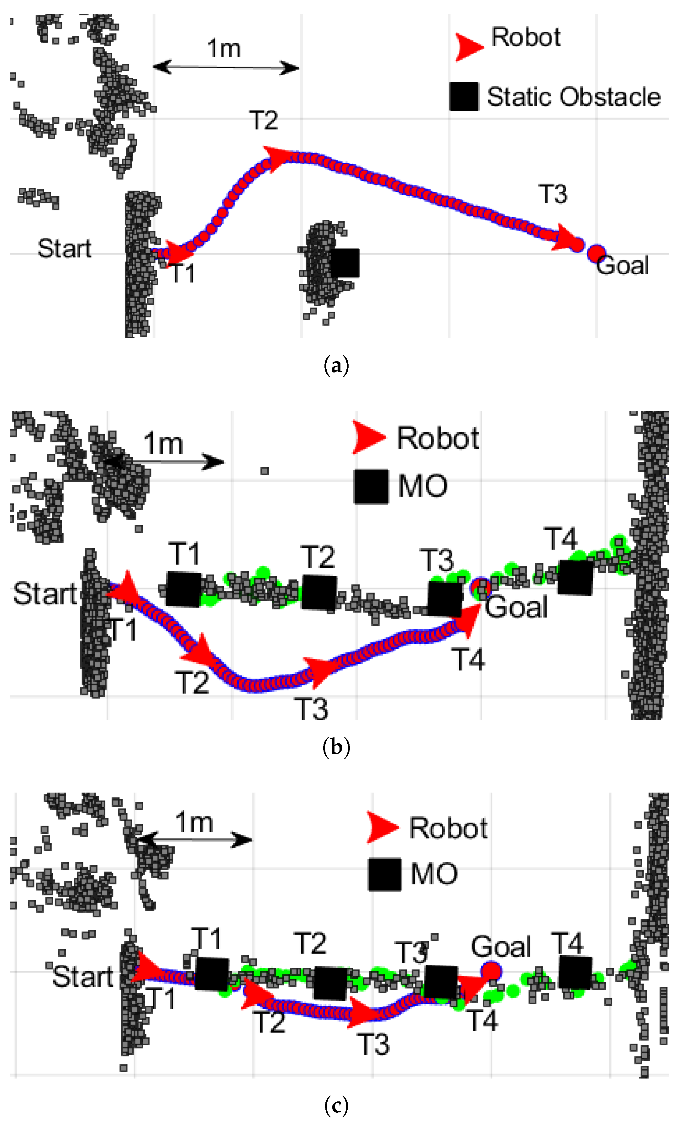
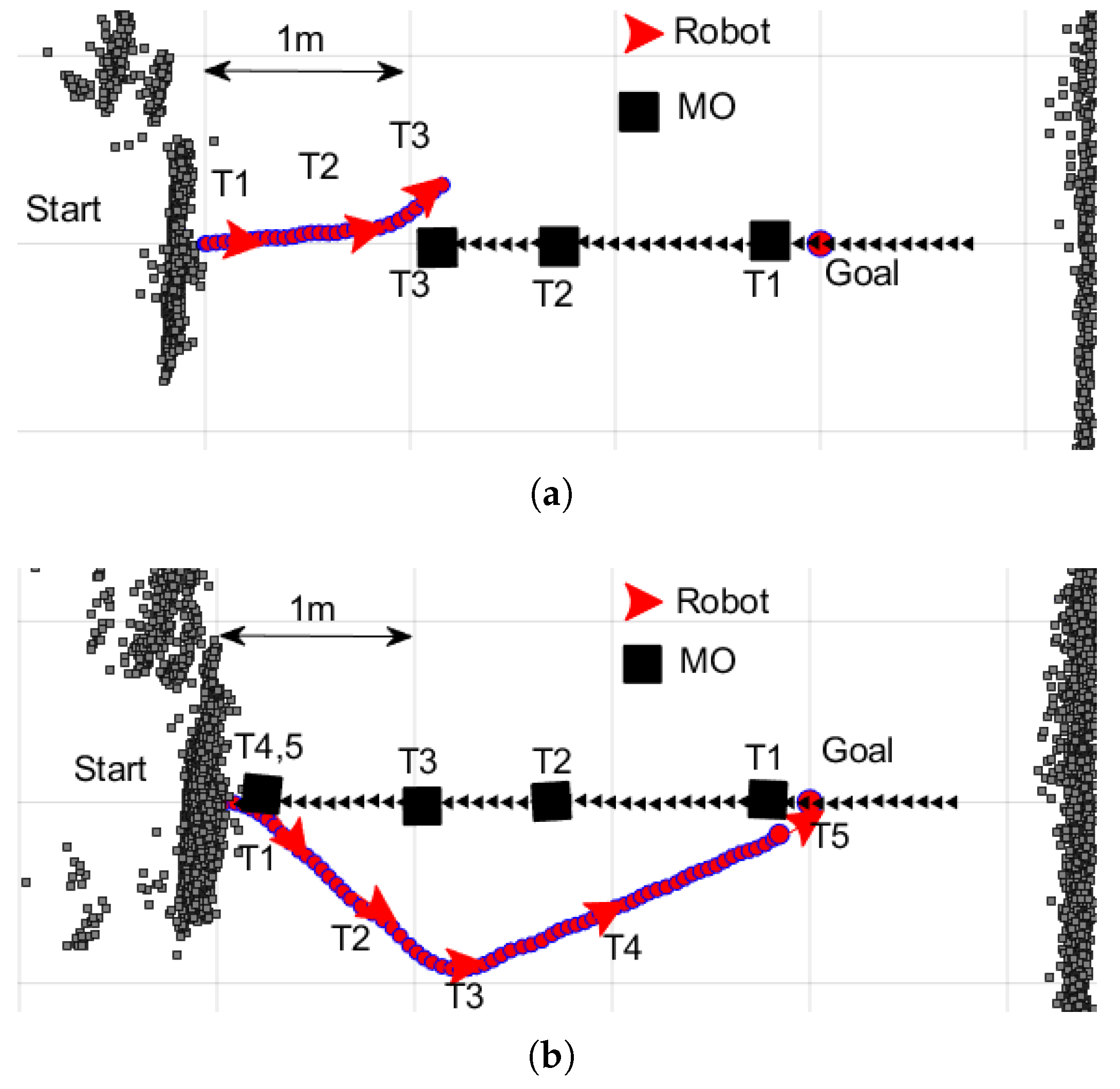
In this experiment, the robot’s starting point was recorded as (0,0), the goal location was (300,0), the MO’s starting point was (27,0), and the MO’s velocity was maintained at 6.3 cm/s. The robot’s maximum allowed velocity was limited to 4.5 cm/s; see Figure 7a.

Case 1: Basic force-shaping module without the FLC:

The robot and the moving obstacle started moving at the instant labelled “T1” (Figure 7b). At this moment, the distance between the robot and the MO was recorded as 27 cm (the MO was close to the robot). As the MO was very close to the robot, the robot immediately started moving away from the MO; see Figure 7b.

At the instant labelled “T2”, the robot kept moving away from the MO and followed a long path to reach the goal. At the instant labelled “T3”, the robot changed its direction back towards the goal. Once the MO passed the goal, the robot reached the goal safely without any collision at the instant labelled “T4”, Figure 7b. In this experiment, the robot travelled 368 cm in 85.6 s with an average speed of 4.3 cm/s.

Case 2: New force-shaping module with the FLC:

The robot and the moving obstacle started moving at the instant labelled “T1” (Figure 7c). At this moment, the distance between the robot and the MO was recorded as 27 cm (the MO was close to the robot). However, the FLC considers the speed and the direction of the MO’s motions. Consequently, the algorithm allowed the robot to move towards the goal without changing its direction. At the instant labelled “T2”, the robot kept moving on the same direction towards the goal safely behind the MO, Figure 6b. With the influence of the new FCL the robot did not change its direction unnecessarily.

At the instant labelled “T3”, the robot showed a slight deviation from the shortest path (Figure 7c). However, the robot redirected its path towards the goal and reached the goal safely without any collision at the instant labelled “T4”; see Figure 6b. In this experiment, the robot travelled 318 cm in 73.9 s with an average speed of 4.3 cm/s,

Table 1. Summarised test results of Experiment 1.

Parameter	Without FLC	With FLC	Performance Comparison with Respect to Case 2
Travel time	85 s	74 s	14%
Path length	368 cm	318 cm	14%
Avg speed	4.3 cm/s	4.3 cm/s	0%

.

The key findings of this experiment are as follows:

• In this experiment, the MO was moving in front of the robot towards the goal, but the MO had a higher speed. Therefore, the robot should not have problems moving towards the goal. However, the basic force-shaping module gave unnecessarily more weight to the existing free space and pushed the robot away from the MO. On the other hand, the force-shaping module with the new FCL allowed the robot to move towards the goal behind the MO while maintaining a safe distance.
• The basic force-shaping module did not consider the velocity of the moving object when it was shaping the FSFs (the path was like avoiding a static obstacle; see Figure 7a).
• The FCL makes important decisions to increase the efficiency of the algorithm by reducing the time to reach the goal and reducing the path length.
• In this experiment, the robot avoided the obstacle by changing its direction of motion (the basic force-shaping module). On the other hand, the force-shaping module with the FLC did not see the MO as a challenge to the robot.
• The object tracking module allowed the algorithm to know about the states (position, velocity) of the MO accurately. This helped the algorithm successfully complete the navigation task.

3.1.2. Experiment 2: A Moving Obstacle Going to the Start Point from the Goal Point

The main purpose of this experiment was to identify the robot’s behaviour when a fast-moving obstacle continuously challenges the robot by moving towards the robot from the goal. This experiment also showed the improvements of the algorithm after introducing the new FLC. The robot’s behaviour was tested with and without the new FLC while keeping similar environments. The speed of the MO kept increasing until it hit the robot. In both cases, the robot could reach the goal without any collision when the MO’s speed was less than 10 cm/s (when the MO’s speed was more than 10 cm/s, the algorithm without the new FLC failed to avoid the collision). The MO’s speed was maintained at 10 cm/s in the two tests presented in this paper.

In this experiment, the robot’s starting point was recoded as (0,0), the goal’s location was (300,0), the MO’s starting point was (370,0), and the MO’s velocity was maintained at −10 cm/s.

Case 1: Basic force-shaping module without the FLC:

The robot and the moving obstacle started moving at the instant labelled “T1” (Figure 8a). At this moment, the distance between the robot and the MO was recorded as 295 cm (the MO was far from the robot). As the MO was far from the robot, the robot started moving towards the goal with its maximum speed; see Figure 8a.

At the instant labelled “T2”, the robot identified that the MO was close to the robot and started changing its direction. However, the decision was made too late, because the MO obstacle had a high speed (more than twice the robot’s maximum speed).

As a result of the delayed decision-making, the robot collided with the MO at the instant labelled “T3”; see Figure 8a. In this test, the robot could not reach the goal safely.

Case 2: New force-shaping module with the FLC:

The robot and the moving obstacle started moving at the instant labelled “T1”, Figure 8b. At this moment, the distance between the robot and the MO was recorded as 295 cm. The MO was far from the robot, but it was coming towards the robot with higher velocity. The FLC considers the speed and the direction of the MO’s motions. Consequently, the robot started moving away from the MO at T1 as it identified the challenge from the MO.

At the instant labelled “T2” (Figure 8a), the robot kept moving in the same direction with the intention of moving away from the MO. The robot’s prior decision-making allowed the robot to successfully avoid the MO at the instant labelled “T3”. The robot redirected its path towards the goal and reached the goal safely without any collision at the instant labelled “T5”; see Figure 8a. In this experiment, the robot travelled 367 cm in 52 s with an average speed of 7 cm/s; see

Table 2. Summarised test results of Experiment 2.

Parameter	Without FLC	With FLC
Travel time	29 s (did not reach the goal)	52 s
Path length	127 cm (did not reach the goal)	367 cm
Avg speed	4.3 cm/s	7.0 cm/s

.

The key findings of this experiment are as follows:

• In this experiment, the MO was coming towards the robot from the goal with high speed. Therefore, the robot was challenged by the MO, although it was not close to the robot. However, the basic force-shaping module allowed the robot to move towards the goal. On the other hand, force-shaping module with the new FCL immediately changed the robot’s direction to deviate the robot’s path from the path of the MO.
• The basic force-shaping module did not consider the object’s velocity in calculating the FSFs. Consequently, the challenge from the fast MO was not identified earlier. This led the robot towards the collision.
• The FCL took the velocities of the MOs into account. This allowed the robot to make important decisions at the right time to avoid collisions.
• In this experiment, the importance of the FLC was pronounced. The FLC helped the robot make the right decision and avoid collision with high-speed moving obstacles.

3.1.3. Experiment 3: A Moving Obstacle Crosses the Robot’s Path Perpendicularly

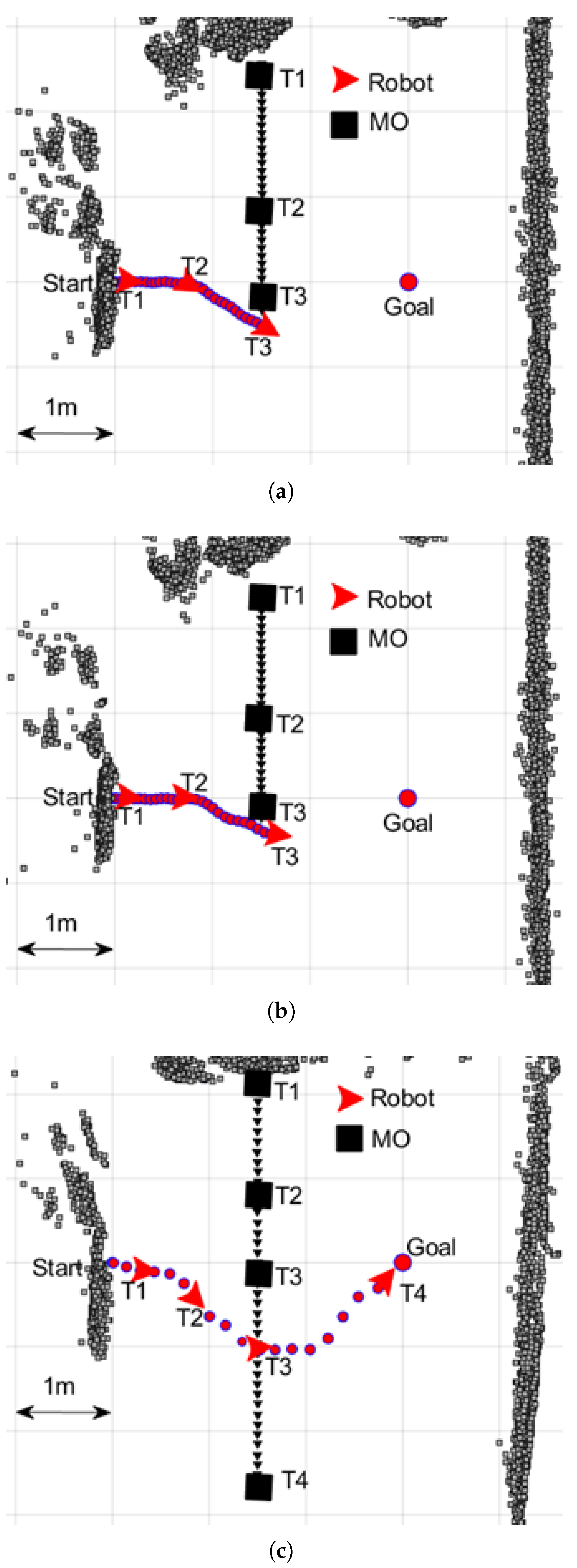
The main purpose of this experiment was to identify the robot’s behaviour when a moving obstacle challenged the robot by moving in a direction perpendicular (−y direction) to the robot’s path; see Figure 9a. This experiment also showed the importance of the prediction module. The robot’s behaviour was tested with and without the prediction module under the same conditions.

Case 1: Navigation without the prediction module:

The robot and the moving obstacle started moving at the instant labelled “T1”. At T1, the MO was moving towards the −y direction. However, the robot immediately started moving towards the goal with its maximum speed; see Figure 9a,b. At the instant labelled “T2”, the algorithm identified that the MO was close to the robot. Then, it started changing its direction. However, the decision was not made in time (the MO had a high speed); see Figure 9a,b. As a result of the delayed decision, the robot collided with the MO at the instant labelled “T3”. In this test, the robot could not reach the goal safely. The same type of decision-making was shown even with the new FLC; see Figure 9b.

Case2: Navigation with the prediction module:

As shown in Figure 9c, the robot and the moving obstacle started moving at the instant labelled “T1”. At T1, the MO was moving towards the −y direction. Although the MO was far from the robot and had a zero velocity component towards the robot’s direction, the prediction module immediately identified that the free space in the robot to goal direction was decreasing. The DOPP module always checks the future growth and diminution of free spaces to help the algorithm make smart decisions. By the influence of the DOPP module, the robot started moving away from the robot to goal path, soon after starting the journey. At the instant labelled “T2”, the robot started moving further in the −y direction (the prediction module influenced the robot with a higher weight). The robot’s prior understanding of future environments allowed the robot to successfully avoid the MO at the instant labelled “T3”. The robot redirected its path towards the goal and reached the goal safely without collision at the instant labelled “T4”, Figure 9c. In this experiment, the robot travelled 372 cm in 88 s with an average speed of 4.2 cm/s,

Table 3. Summarised test results of Experiment 3.

Parameter	Without FLC and DOPP	With FLC and without DOPP	With FLC and DOPP
Travel time	Did not reach the goal	Did not reach the goal	88 s
Path length	Did not reach the goal	Did not reach the goal	372 cm
Avg speed	4.3 cm/s	4.3 cm/s	4.3 cm/s

.

The key findings of this experiment are as follows:

• In this experiment, the MO was moving fast in the direction perpendicular to the robot’s initial motion (start to goal direction). Therefore, the force-shaping module did not see any sector velocity component from the MO (as the velocity was perpendicular to the robot’s to goal direction) nor any obstacle in between the robot and the goal.
• The algorithm without the prediction module made decisions based only on the current circumstances in the robot’s surrounding. Consequently, the robot could not change its direction and kept moving towards the goal at the beginning of the journey (Key Finding 1: the algorithm did not realize the change of the MO). This was the costly decision that led the robot to a collision.
• The algorithm with the prediction module makes decisions not only based on the robot’s current surroundings, but also considering the future environments. This allowed the robot to identify future growth and diminishing of the free space. As a result, the robot could make prior decisions. This helped the robot reach the goal safely without any collision.
• In this experiment, the importance of the prediction module was verified. It enabled the robot to make early decisions when the robot is dealing with some special cases.

3.1.4. Experiment 4: The Robot Reaches the Goal despite Two Moving Obstacles Simultaneously Challenging the Robot

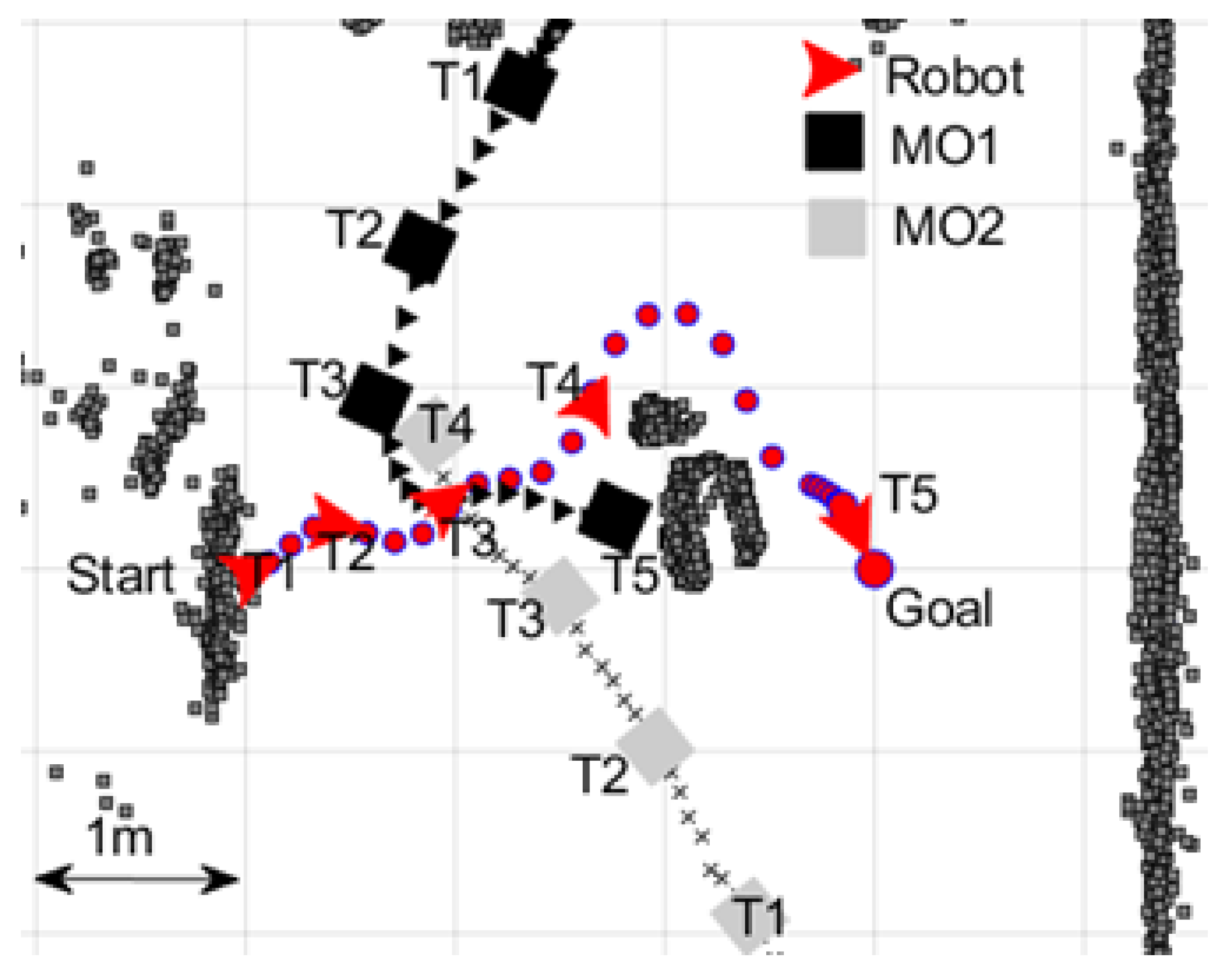
The main purpose of this experiment was to identify the robot’s behaviour in a random environment with multiple moving obstacles and static obstacles. In this experiment, two static obstacles and two moving obstacles were used to challenge the robot. The first moving obstacle MO1 changed its speed and direction rapidly to test the algorithm’s capabilities. The second moving obstacle MO2 tried to maintain a constant velocity during the experiment (however, there were slight directional and speed variations). For this experiment, the full-strength algorithm was used (with prediction and the FCL).

The robot started moving at the instant labelled “T1”, and the two moving obstacles started moving 3 s before the robot. At this moment, MO1 was coming towards the robot with a very slow speed (0.2 cm/s). MO2 was coming towards the robot with a higher speed (4.2 cm/s) compared to MO1. At the beginning, due to the challenge of MO2, the robot moved towards the (+x, +y) direction with the intention of passing the MO2 in front. However, during T1 and T2, the MO1 increased its speed to a reasonably challenging level (4.5 cm/s). Therefore, the robot stopped moving further in the (+x, +y) direction and stared moving in the (+x) direction (T2 in Figure 10). During this time instant, T2 to T3, the robot was challenged by MO1 and MO2. The prediction module and advanced force-shaping module influenced the algorithm to make critical decisions to win this challenge. As a result of good decision-making, the robot could safely pass in between MO1 and MO2 at the time instant T3.

After successfully avoiding the collisions with MO1 and MO2, the robot’s path was interrupted by two closely passing static obstacles. The robot chose to go around the two static obstacles instead of going in between them (the safety boundary technique used in the FSH module influenced this decision). While passing the static obstacles, the robot increased its speed and reached the goal at time instant T5.

In this experiment, the robot travelled 495 cm in 117 s with an average speed of 4.2 cm/s.

The key findings of this experiment are as follows:

• The tacking module estimated the locations and velocities of the moving obstacles accurately.
• The prediction module could predicted the future increasing and diminishing free space based on the predictions of the future locations of the moving obstacles and the robot.
• The algorithm was able to handle challenging situations where multiple moving objects challenged the robot at the same time.
• The new Agoraphilic algorithm can successfully navigate robots in unknown dynamic environments.

3.1.5. Experiment 5: The Robot Reaches the Goal despite Three Moving Obstacles Simultaneously Challenging the Robot and Pushing the Robot towards a Trap

The main purpose of this experiment was to characterise the robot’s behaviour when placed in a random environment with multiple moving and static obstacles incorporating traps. The experimental scenario included one static obstacle and three moving obstacles designed to challenge the robot. The first moving obstacle, MO1, changed its speed and direction rapidly to test the algorithm’s dynamic capabilities. The second, MO2, was programmed to maintain a constant velocity during the experiment. The third, MO3, slightly changed its speed and direction during the experiment. For this test, the full algorithm, including prediction and the FLC, was used.

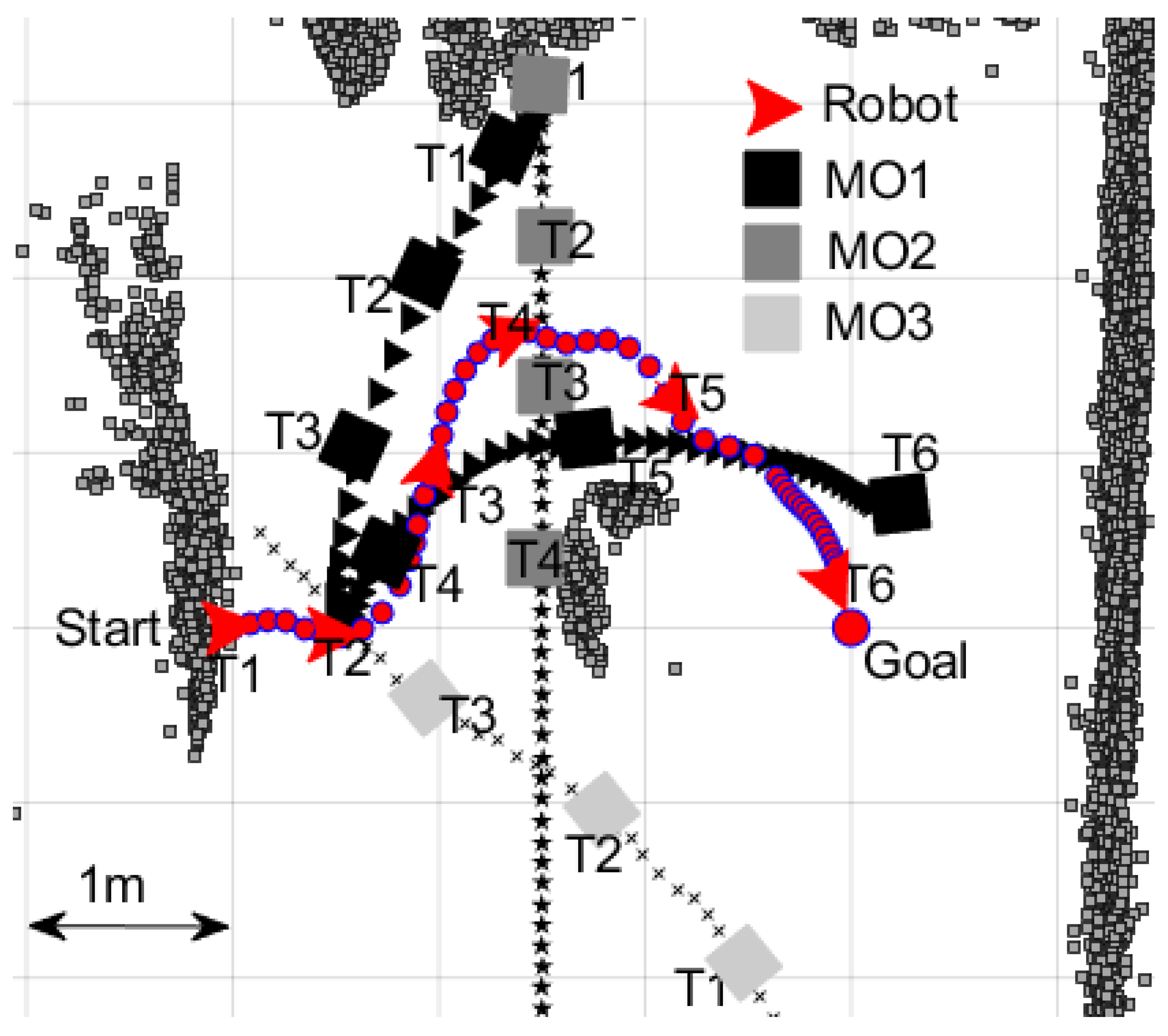
Figure 11 illustrates the trajectories that resulted from this scenario. The robot, MO1, and MO2 started moving at the instant labelled “T1”. Moving Object 3 started moving 3 s before the time instant T1. At this moment, MO1 and MO3 were coming towards the robot. The robot moved in the +x direction to avoid any collisions with MO1 and MO3.

At the time instant T2, the robot had four possible choices:

• Move in the (+x, −y) direction to pass in front of MO2 and reach the goal in the shortest path.
• Reduce its speed and wait for MO2 to pass.
• Go forward towards the goal.
• Move in the (+x, +y) direction (towards the converging MO1 and MO2).

The new force-shaping module with the FLC operating identified the challenge from MO3 (although it was distant from the robot, it was rapidly approaching the robot in the (+x, −y) direction) and stopped the robot from moving towards the (+x, −y) direction. The prediction module also supported this decision. The second option was eliminated by the prediction module as it identified that the robot would be hit by MO1 and MO2 if the robot slowed down. The force-shaping module did not choose the third option as there remained a static obstacle between the robot and the goal. The new Agoraphilic algorithm picked the fourth option, although it is a more complicated solution. The algorithm successfully manoeuvred the robot through the time-varying free space passage in between MO1 and MO2 during time interval T2–T4. During this time interval, the force-shaping module gave accurate directions and avoided any incorrect decisions that may have driven the robot to a trap or resulted in a collision.

At time instant T4, the robot avoided the major challenges from MO1 and MO2 and started changing its direction towards the goal. However, MO1 started crossing the robot’s path again between T4 and T6. The robot slightly changed its path at time instant T5 as a result of this influence from MO1. Finally, the robot reached the goal safely at time instant T6.

In this experiment, the robot travelled 557.0 cm in 133 s with an average speed of 4.2 cm/s.

The key findings of this experiment are as follows:

• The importance of the new FLC, even in the presence of the prediction module, was clearly shown in this experiment.
• The algorithm was able to identify and implement successful decisions in complex environments.
• The force-shaping module could select the robot’s pathway precisely to navigate through narrow time-varying free space corridors.
• The new Agoraphilic algorithm could successfully navigate robots in unknown dynamic environments with traps.

3.2. Experimental Comparison of the Proposed Algorithm with Other Recent Approaches

This subsection presents three experiments that were conducted to compare the ANADE with three other recent navigation algorithms.

3.2.1. Comparison of the ANADE with the Matrix-Binary-Code-Based Genetic Algorithm

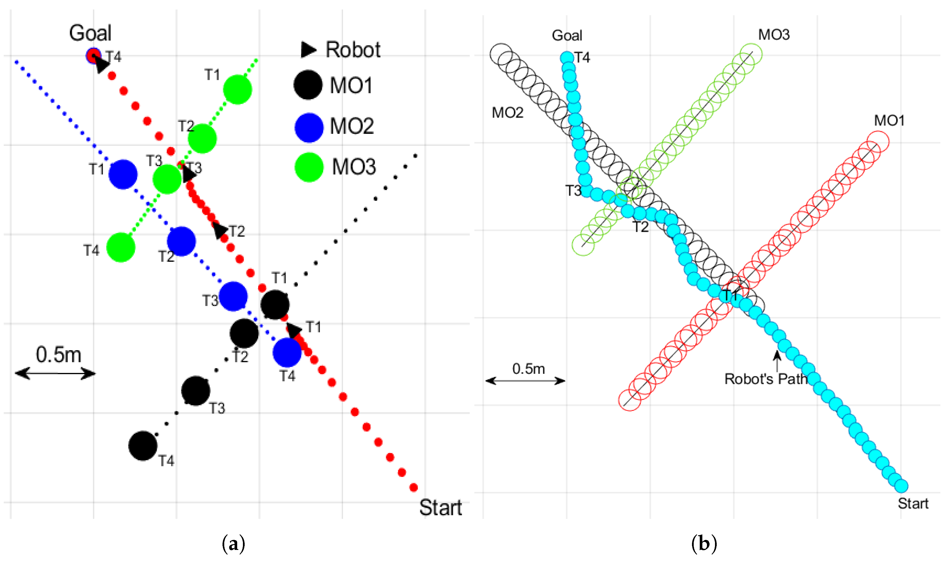
In this experiment, the environmental setup was developed to match the environment that was used in [9]. This was to compare the results under the same conditions. Three moving obstacles were used in this setup. By comparing the results of the ANADE and matrix-binary-code-based genetic algorithm (MBCGA), we noticed that there were two different decisions at time instant T1 (Figure 12):

• ANADE—slowed down the robot, and MO1 was enabled to pass the robot.
• MBCGA—changed the robot’s moving direction and passed the MO1.

In this case, the ANADE reduced the robot’s speed, enabling the MO1 to pass as the free space was diminishing, which was enabled through the embedded prediction algorithm. Consequently, the robot with the ANADE easily avoided the challenge from MO2 at time instant T2. On the other hand, the robot with the MBCGA method had to move further in the x-direction to avoid MO2. In addition, the two algorithms made different decisions at time instant T3 as well; see Figure 12. Overall, the decisions made by the ANADE allowed the robot to use a shorter path with 66% fewer direction changes to reach the goal compared to the MBCGA; see Figure 12.

3.2.2. Comparison of the ANADE with the Fuzzy Wind-Driven Optimization Algorithm

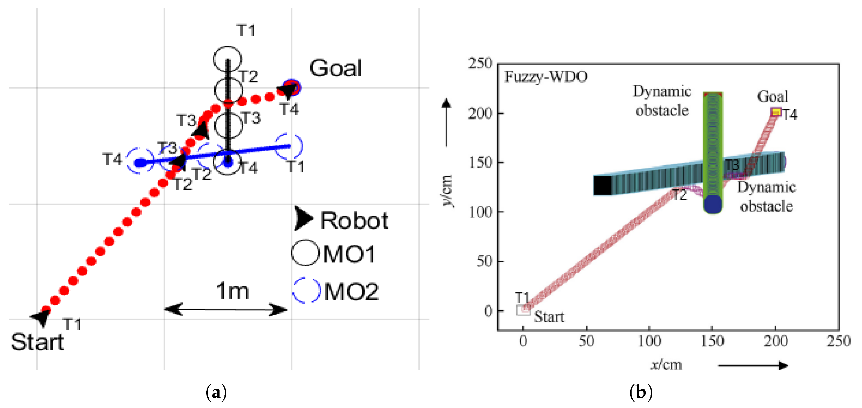
In this experiment, the environmental setup was developed to match the experimental setup used in [12]. Hence, the experiment was conducted with two moving obstacles under similar conditions. It can be seen in this experiment that the robot with the ANADE and the robot with the fuzzy wind-driven optimization algorithm (FWDOP) made two different decisions at time instant T2 (Figure 13):

• ANADE—increased the speed of the robot and passed MO2 at its front.
• FWDOA—turned towards the (+x, −y) direction.

In this case, the ANADE increased the robot’s speed, enabling the robot to pass MO2, as the free space on robot’s left side was not stationary and DO2 was moving slowly compared to the robot. Therefore, the robot with the ANADE algorithm managed to easily avoid the challenge imposed by MO2 at time instant T3, without any direction change. On the other hand, the robot with the FWDOA [12] had to change its direction towards the +x direction to avoid DO2. Furthermore, at time instant T3, the two algorithms made different decisions.

Overall, the decisions made by the ANADE allowed the robot to use a shorter path with 25% fewer direction changes to reach the goal compared to the FWDOA; see Figure 13.

3.2.3. Comparison of the ANADE with an Improved APF Algorithm Developed Based on the Transferable Belief Model

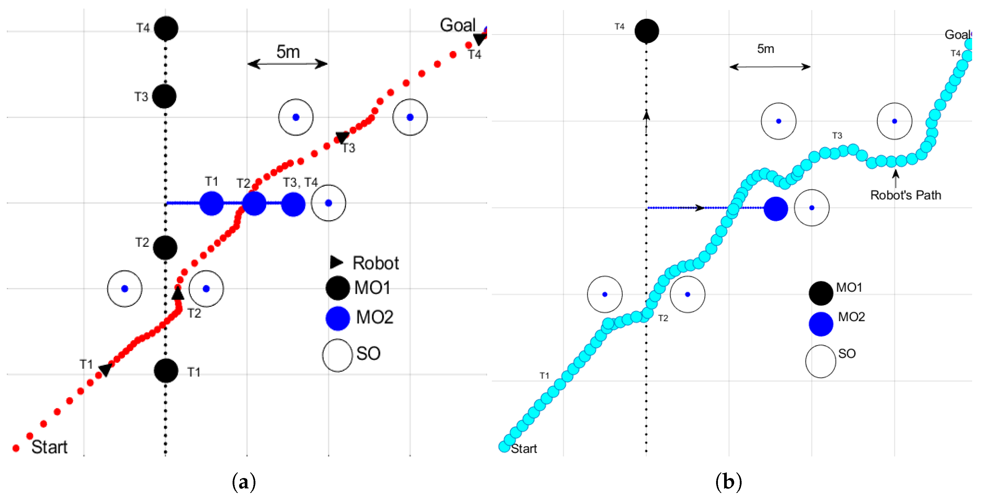
In this experiment, the environmental setup was developed according to an experimental setup that was used in [33] to compare the results under the same conditions. Two moving obstacles and five static obstacles were used in this experiment. It was observed from this bench-marking that the ANADE algorithm used a shorter path and 33% fewer direction changes to reach the goal compared to the improved APF algorithm (APF algorithm based on the transferable belief model (APF-TBM)); see Figure 14.

3.3. A Qualitative Comparison between the Proposed Algorithm with Recent Navigation Approaches

A qualitative comparison between some of the recently published methods is shown in

Table 4. A qualitative comparison between the proposed navigation algorithm with other approaches.

Algorithm [Ref.]	Base Concept	Tracking	Prediction	Velocity for Decision-Making	Unknown Dynamic Environments	Experimental Validation
[12]	Fuzzy Logic	No	No	No	Yes	Yes
[9]	Genetic Algorithm	No	No	No	Yes	Yes
[33]	APF	Yes	No	Yes	Yes	Yes
[34]	Bacterial Foraging	No	No	No	Yes	No
[35]	Dynamic Window Approach	No	No	No	Yes	Yes
[36]	APF	No	No	No	Yes	No
[37]	APF	No	Yes	Yes	Yes	No
[38]	APF	No	Yes	Yes	Yes	No
[13]	GDP	No	No	No	Yes (but very slow MOs. MO vel <0.5 cm/s)	Yes
ANADE	Agoraphilic (Free-Space Attraction)	Yes	Yes	Yes	Yes	Yes

. A set of cardinally important features for mobile robot navigation in unknown dynamic environments was used in this qualitative comparison.

4. Conclusions

The primary aims of this research work were to develop a novel navigation algorithm capable of operating in dynamic environments using the free space concept and to verify its performance experimentally. The new Agoraphilic navigation algorithm in dynamic environments (ANADE) presented in this paper is a local path planner designed to navigate mobile robots in unknown static, as well as dynamic environments that exhibit high levels of uncertainty. A controller, based on fuzzy logic, was developed to provide optimal navigational solutions at a low computational cost as a pivotal part of the new Agoraphilic algorithm. The effectiveness of the ANADE was further improved by incorporating the velocity vectors of moving obstacles in the decision-making. The tracking module was able to estimate the position and velocities of unknown moving obstacles accurately. Further, the algorithm’s dynamic object position prediction methodology describes the robot’s future environments accurately.

Five experiments and three simulations were designed and executed to demonstrate the effectiveness of the algorithm and bench-mark the algorithm against other recently published methods. The experimental test results clearly demonstrated the effectiveness of the novel Agoraphilic algorithm with the embedded fuzzy-based force-shaping module. The experiments also showed that object tracking and prediction helped the robot reach its goal safely in dynamically challenging conditions that may constitute traps. The inclusion of moving obstacle velocity vectors within the prediction methodology further refined the algorithm and significantly improved its effectiveness in dynamic environments. The comparison tests of the ANADE with other methods proved that the ANADE makes human-like decisions to keep minimal direction changes and a shorter path to reach the goal. The new algorithm demonstrated enhanced capabilities to successfully navigate mobile robots through complicated dynamic environments without collisions and at a level of performance superior to previously developed navigational algorithms.

References

1. Liu, W.; Li, Z.; Sun, S.; Gupta, M.K.; Du, H.; Malekian, R.; Sotelo, M.A.; Li, W. Design a Novel Target to Improve Positioning Accuracy of Autonomous Vehicular Navigation System in GPS Denied Environments. IEEE Trans. Ind. Inform. 2021, 17, 7575–7588. [Google Scholar] [CrossRef]
2. Gao, Y.; Chien, S. Review on space robotics: Toward top-level science through space exploration. Sci. Robot. 2017, 2, eaan5074. [Google Scholar] [CrossRef] [PubMed] [Green Version]
3. Rangapur, I.; Prasad, B.S.; Suresh, R. Design and Development of Spherical Spy Robot for Surveillance Operation. Procedia Comput. Sci. 2020, 171, 1212–1220. [Google Scholar] [CrossRef]
4. Patil, D.; Ansari, M.; Tendulkar, D.; Bhatlekar, R.; Pawar, V.N.; Aswale, S. A Survey On Autonomous Military Service Robot. In Proceedings of the 2020 International Conference on Emerging Trends in Information Technology and Engineering (ic-ETITE), Vellore, India, 24–25 February 2020; pp. 1–7. [Google Scholar] [CrossRef]
5. Huang, X.; Cao, Q.; Zhu, X. Mixed path planning for multi-robots in structured hospital environment. J. Eng. 2019, 2019, 512–516. [Google Scholar] [CrossRef]
6. Kayacan, E.; Kayacan, E.; Ramon, H.; Kaynak, O.; Saeys, W. Towards Agrobots: Trajectory Control of an Autonomous Tractor Using Type-2 Fuzzy Logic Controllers. IEEE/ASME Trans. Mechatronics 2015, 20, 287–298. [Google Scholar] [CrossRef]
7. Sawadwuthikul, G.; Tothong, T.; Lodkaew, T.; Soisudarat, P.; Nutanong, S.; Manoonpong, P.; Dilokthanakul, N. Visual Goal Human-Robot Communication Framework with Few-Shot Learning: A Case Study in Robot Waiter System. IEEE Trans. Ind. Inform. 2021, 18, 1883–1891. [Google Scholar] [CrossRef]
8. Hewawasam, H.S.; Ibrahim, M.Y.; Appuhamillage, G.K. Past, Present and Future of Path-Planning Algorithms for Mobile Robot Navigation in Dynamic Environments. IEEE Open J. Ind. Electron. Soc. 2022, 3, 353–365. [Google Scholar] [CrossRef]
9. Patle, B.; Parhi, D.; Jagadeesh, A.; Kashyap, S.K. Matrix-Binary Codes based Genetic Algorithm for path planning of mobile robot. Comput. Electr. Eng. 2018, 67, 708–728. [Google Scholar] [CrossRef]
10. Engedy, I.; Horváth, G. Artificial neural network based mobile robot navigation. In Proceedings of the 2009 IEEE International Symposium on Intelligent Signal Processing, Kanazawa, Japan, 7–9 December 2009; pp. 241–246. [Google Scholar]
11. Niu, H.; Ji, Z.; Arvin, F.; Lennox, B.; Yin, H.; Carrasco, J. Accelerated sim-to-real deep reinforcement learning: Learning collision avoidance from human player. In Proceedings of the 2021 IEEE/SICE International Symposium on System Integration (SII), Iwaki, Japan, 11–14 January 2021; pp. 144–149. [Google Scholar]
12. Pandey, A.; Parhi, D.R. Optimum path planning of mobile robot in unknown static and dynamic environments using Fuzzy-Wind Driven Optimization algorithm. Def. Technol. 2017, 13, 47–58. [Google Scholar] [CrossRef]
13. Zhou, X.; Wang, Z.; Ye, H.; Xu, C.; Gao, F. Ego-planner: An esdf-free gradient-based local planner for quadrotors. IEEE Robot. Autom. Lett. 2020, 6, 478–485. [Google Scholar] [CrossRef]
14. Na, S.; Niu, H.; Lennox, B.; Arvin, F. Bio-Inspired Collision Avoidance in Swarm Systems via Deep Reinforcement Learning. IEEE Trans. Veh. Technol. 2022, 71, 2511–2526. [Google Scholar] [CrossRef]
15. Mohanta, J.C.; Keshari, A. A knowledge based fuzzy-probabilistic roadmap method for mobile robot navigation. Appl. Soft Comput. 2019, 79, 391–409. [Google Scholar] [CrossRef]
16. Patle, B.; Babu L, G.; Pandey, A.; Parhi, D.; Jagadeesh, A. A review: On path planning strategies for navigation of mobile robot. Def. Technol. 2019, 15, 582–606. [Google Scholar] [CrossRef]
17. Lee, D.H.; Lee, S.S.; Ahn, C.K.; Shi, P.; Lim, C. Finite Distribution Estimation-based Dynamic Window Approach to Reliable Obstacle Avoidance of Mobile Robot. IEEE Trans. Ind. Electron. 2020, 68, 9998–10006. [Google Scholar] [CrossRef]
18. Li, G.; Tamura, Y.; Yamashita, A.; Asama, H. Effective improved artificial potential field-based regression search method for autonomous mobile robot path planning. Int. J. Mechatronics Autom. 2013, 3, 141–170. [Google Scholar] [CrossRef] [Green Version]
19. Babinec, A.; Duchon, F.; Dekan, M.; Mikulova, Z.; Jurisica, L. Vector Field Histogram* with look-ahead tree extension dependent on time variable environment. Trans. Inst. Meas. Control 2018, 40, 1250–1264. [Google Scholar] [CrossRef]
20. Saranrittichai, P.; Niparnan, N.; Sudsang, A. Robust local obstacle avoidance for mobile robot based on Dynamic Window approach. In Proceedings of the 2013 10th International Conference on Electrical Engineering/Electronics Computer, Telecommunications and Information Technology, Krabi, Thailand, 15–17 May 2013; pp. 1–4. [Google Scholar] [CrossRef]
21. Liu, C.; Lee, S.; Varnhagen, S.; Tseng, H.E. Path planning for autonomous vehicles using model predictive control. In Proceedings of the 2017 IEEE Intelligent Vehicles Symposium (IV), Los Angeles, CA, USA, 11–14 June 2017; pp. 174–179. [Google Scholar] [CrossRef]
22. Babic, B.; Nesic, N.; Miljkovic, Z. A review of automated feature recognition with rule-based pattern recognition. Comput. Ind. 2008, 59, 321–337. [Google Scholar] [CrossRef]
23. Kovács, B.; Szayer, G.; Tajti, F.; Burdelis, M.; Korondi, P. A novel potential field method for path planning of mobile robots by adapting animal motion attributes. Robot. Auton. Syst. 2016, 82, 24–34. [Google Scholar] [CrossRef]
24. Ibrahim, M.Y.; McFetridge, L. The Agoraphilic algorithm: A new optimistic approach for mobile robot navigation. In Proceedings of the 2001 IEEE/ASME International Conference on Advanced Intelligent Mechatronics, Proceedings (Cat. No. 01TH8556), Como, Italy, 8–12 July 2001; Volume 2, pp. 1334–1339. [Google Scholar] [CrossRef]
25. Dai, X.; Li, C.K.; Rad, A. An approach to tune fuzzy controllers based on reinforcement learning for autonomous vehicle control. IEEE Trans. Intell. Transp. Syst. 2005, 6, 285–293. [Google Scholar] [CrossRef]
26. Kamil, F.; Hong, T.S.; Khaksar, W.; Moghrabiah, M.Y.; Zulkifli, N.; Ahmad, S.A. New robot navigation algorithm for arbitrary unknown dynamic environments based on future prediction and priority behaviour. Expert Syst. Appl. 2017, 86, 274–291. [Google Scholar] [CrossRef]
27. Bahraini, M.S.; Bozorg, M.; Rad, A.B. SLAM in dynamic environments via ML-RANSAC. Mechatronics 2018, 49, 105–118. [Google Scholar] [CrossRef]
28. Hewawasam, H.S.; Ibrahim, M.Y.; Kahandawa, G.; Choudhury, T.A. Comparative Study on Object Tracking Algorithms for mobile robot Navigation in GPS-denied Environment. In Proceedings of the 2019 IEEE International Conference on Industrial Technology (ICIT), Melbourne, Australia, 13–15 February 2019; pp. 19–26. [Google Scholar] [CrossRef]
29. Elnagar, A. Prediction of moving objects in dynamic environments using Kalman filters. In Proceedings of the Proceedings 2001 IEEE International Symposium on Computational Intelligence in Robotics and Automation (Cat. No. 01EX515), Banff, AB, Canada, 29 July–1 August 2001; pp. 414–419. [Google Scholar] [CrossRef]
30. Hewawasam, H.S.; Ibrahim, M.Y.; Kahandawa, G.; Choudhury, T.A. Agoraphilic navigation algorithm in dynamic environment with obstacles motion tracking and prediction. Robotica 2022, 40, 329–347. [Google Scholar] [CrossRef]
31. McFetridge, L.; Ibrahim, M.Y. Behavior fusion via free space force-shaping. In Proceedings of the IEEE International Conference on Industrial Technology, Shanghai, China, 22–25 August 2003; Volume 2, pp. 818–823. [Google Scholar] [CrossRef]
32. Hewawasam, H.S.; Ibrahim, M.Y.; Appuhamillage, G.K.; Choudhury, T.A. Agoraphilic Navigation Algorithm Under Dynamic Environment. IEEE/ASME Trans. Mechatronics 2022, 27, 1727–1737. [Google Scholar] [CrossRef]
33. Yaonan, W.; Yimin, Y.; Xiaofang, Y.; Yi, Z.; Yuanli, Z.; Feng, Y.; Lei, T. Autonomous mobile robot navigation system designed in dynamic environment based on transferable belief model. Measurement 2011, 44, 1389–1405. [Google Scholar] [CrossRef]
34. Hossain, M.A.; Ferdous, I. Autonomous robot path planning in dynamic environment using a new optimization technique inspired by bacterial foraging technique. Robot. Auton. Syst. 2015, 64, 137–141. [Google Scholar] [CrossRef]
35. Xin, J.; Jiao, X.; Yang, Y.; Liu, D. Visual navigation for mobile robot with Kinect camera in dynamic environment. In Proceedings of the 2016 35th Chinese Control Conference (CCC), Chengdu, China, 27–29 July 2016; pp. 4757–4764. [Google Scholar] [CrossRef]
36. Bodhale, D.; Afzulpurkar, N.; Thanh, N.T. Path planning for a mobile robot in a dynamic environment. In Proceedings of the 2008 IEEE International Conference on Robotics and Biomimetics, Bangkok, Thailand, 14–17 December 2009; pp. 2115–2120. [Google Scholar] [CrossRef]
37. Huang, L. Velocity planning for a mobile robot to track a moving target-a potential field approach. Robot. Auton. Syst. 2009, 57, 55–63. [Google Scholar] [CrossRef]
38. Jaradat, M.A.K.; Garibeh, M.H.; Feilat, E.A. Autonomous mobile robot dynamic motion planning using hybrid fuzzy potential field. Soft Comput. 2012, 16, 153–164. [Google Scholar] [CrossRef]
Figure 1. A block diagram of the fuzzy logic controller (FLC).
Machines 10 01085 g001
Figure 2. Input membership functions of the fuzzy controller.
Machines 10 01085 g002
Figure 3. Output membership functions of the fuzzy controller.
Machines 10 01085 g003
Figure 4. FSH used to derive the membership function for input θ d i f f .
Machines 10 01085 g004
Figure 5. Experimental setup.
Machines 10 01085 g005
Figure 6. RGB and depth images captured from Real Sense camera. (a) RGB image. (b) Depth image.
Machines 10 01085 g006
Figure 7. The robot’s paths observed in Experiment 1 with different configurations. The robot’s and obstacle’s locations at three different time instants are shown as T1–T3. (a) With a static obstacle (this configuration creates a local minimum for the APF method), (b) moving obstacle without the new FLC, and (c) moving obstacle with the new FLC.
Machines 10 01085 g007
Figure 8. The robot’s paths observed in Experiment 2 with different configurations. The robot’s and obstacle locations at three different time instants are shown as T1–T3. (a) Moving obstacle without the new FLC. (b) Moving obstacle with the new FLC.
Machines 10 01085 g008
Figure 9. The robot’s paths observed in Experiment 3 with different configurations. The robot’s and obstacle’s locations at four different time instants are shown as T1–T4. (a) Robot without the new FCL and the DOPP module, (b) robot with the new FCL and without the DOPP module, and (c) robot with the new FCL and the DOPP module.
Machines 10 01085 g009
Figure 10. The robot’s observed path in Experiment 4. The locations of the robot and moving obstacles (MO1–MO2) are shown at five different time instants (T1–T5).
Machines 10 01085 g010
Figure 11. The robot’s observed path in Experiment 5. The locations of the robot and moving obstacles (MO1–MO3) are shown at six different time instants (T1–T6).
Machines 10 01085 g011
Figure 12. The ANADE and MBCGA. The robot’s and obstacles’ locations at four different time instants, T1–T4. (a) The robot’s path with the ANADE. (b) The robot’s path with the MBCGA.
Machines 10 01085 g012
Figure 13. The ANADE and FWDOA. The robot’s and obstacles’ locations at four different time instants, T1–T4. (a) The robot’s path with the ANADE. (b) The robot’s path with the FWDOA [12].
Machines 10 01085 g013
Figure 14. The ANADE and APF-TBM. The robot’s and obstacles’ locations at four different time instants T1–T4. (a) The robot’s path with the ANADE. (b) The robot’s path with the APF-TBM.
Machines 10 01085 g014