Speed Tracking for IFOC Induction Motor Speed Control Using Hybrid Sensorless Speed Estimator Based on Flux Error for Electric Vehicles Application

Abstract

This paper presents hybrid sensorless speed tracking by an indirect field-oriented control (IFOC) for an induction motor (IM). The sensorless model is based on an improved virtual estimation topology model to predict the virtual speed and flux of the IM using stator current components. The hybrid sensorless model, defined as a modification of voltage with a rotor flux-oriented current model, was also implemented with proportional-integral (PI) control for comparison with the conventional voltage model (CVM). The suggested adaptive mechanism for PI control in the hybrid estimator was able to compensate for the back-EMF error from the rotor flux-oriented current model into the voltage model and change the air gap flux of the IM. An accurate rotor flux position was estimated and used to estimate the speed with low speed error. This IFOC model, with various speed change references, was tested in a simulation environment by using the MATLAB/Simulink program. The proposed hybrid estimator was tested in two different EV operations, which were reverse and forward operations. The effectiveness of the proposed estimator was analyzed for its transient and steady-state performances based on settling time, recovery time and the overshoot and speed error percentages. All the results were in good agreement in terms of the stability of the speed and current controller with minimum speed error obtained, where the average errors were 0.08% and 0.16% for high speed and lower speed, respectively.

1. Introduction

A high-performance induction motor (IM) requires various special characteristics, such as robustness against parameter variation, a stable system during operation, faster load disturbance rejection and also faster dynamic responses. The use of an IM in industrial applications is generally based on its main advantages, which are high reliability and a wide range of speed [1]. Due to its simple construction without magnets on its rotors, the trend of IM application will increase in the coming years because of its low cost.

The first electric vehicle (EV) was built in 1839, but the IM application in the transportation industry has been gaining acceptability in recent years [2]. EVs will be a major transportation mechanism due to the increase in concerns over global warming and due to energy efficiency plans that have led car manufacturers to deploy more IMs in EVs, compared with DC motors or permanent magnet synchronous motors (PMSMs). IMs in the EV industry are used over other types of motors because of the possibility of regenerative braking in the four-quadrant operation [3].

A key condition toward a wider application of the IM is vector control, which is mostly used to control the IM in advance with a sensorless mode. The essential feature of vector control is the ability to have decoupled control between the flux and the torque generated by the stator currents with direct and indirect field-oriented control methods, which reflect the motor’s speed response [4]. Therefore, to realize the sensorless mode, an estimation technique could be used to estimate the speed of the IM, which would eliminate the use of a speed sensor and consequently reduce the maintenance cost, hence making the EV a smart system. Various estimation techniques have been developed to obtain the minimum speed error and reduce the computational burden in the estimating processes, such as the current model, voltage model, fuzzy logic and Kalman filter [5,6,7,8]. These techniques have excellent performance depending on how they are applied, but in some cases the speed estimation is still unsatisfactory due to the large speed error produced.

Vector control for motor operation is normally achieved by using a proportional-integral (PI) controller either for the speed or current control. As discussed in [9,10,11], a PI controller is used to control the speed with a single estimator of speed and without any adaptation mechanism. However, the weakness of a PI controller is that it cannot compromise with unknown motor parameters, such as stator resistance and inductance, if they are not being considered in the input parameters, which currently are obtained from the speed input sensor. These parameters vary during operation due to temperature changes and the magnetic saturation effect, which deteriorate the IM performance and make it operate at low efficiency [12]. The issue was resolved in [13,14,15], where a tuning method (PI tuner) was used to tune the controller’s response. The tuning process focused on the variable speed operation without considering the load disturbance rejection. This could harm the IM, where the cogging torque reduces the IM performance and makes it operate below the base speed [16]. Various tuning methods have been developed by introducing currently trending methods, such as fuzzy logic, Kalman filters, neural networks and neuro-fuzzy, in order to have good load disturbance rejection [17,18,19,20,21,22]. However, due to complexities, few have been applied in IM vector control. These complexities give a computational burden to the control system, which causes the overlapping loop problem between the controllers [23].

In this paper, an indirect field-oriented control (IFOC) was adopted with a sensorless model and with the PI speed and current controllers to control the speed and torque of the IM. Here, the sensorless model took the function of the speed sensor. The current and voltage coming to the IM became the inputs of the speed estimation model, which were based on the parameters of the IM. A pre-compensating method was introduced in the current controller to balance the control operation at a wide range of speed so that the ripples on the current response could be reduced. In order to resolve the load disturbance rejection, a hybrid topology based on the modified voltage model and the rotor flux-oriented current model was applied to estimate the feedback speed by the stator voltage and current components, which responded according to the load torque disturbances. The results obtained were analyzed for controller stability to seek the minimum speed error.

This paper is organized as follows: In Section 2 and Section 3, the dynamic modeling of the IM and the concept of field-oriented control (FOC) are described, respectively. In Section 4, the proposed hybrid estimator with the stator flux control as the adaptive mechanism is explained. In Section 5, the stability of the speed and current controllers are determined. In Section 6, the simulation results are analyzed, followed by the performance evaluation and conclusion.

2. Dynamic Modeling of Induction Motor

The space vector method presented in Figure 1 describes the mathematical modeling of the IM. Based on the vector method, s and r are stator and rotor circuits, respectively, and e refers to the synchronously rotating frame, while a, b and c are the axes of the phase system and d and q are direct and quadrature axes with respect to the stator components, respectively. The field angle θ_e is extracted from the time integral of the angular frequency ω_e. By subtracting the slip frequency ω_sl from the field angle, the rotor flux position θ_r can be calculated as:

θ_r = θ_e − θ_sl

(1)

The state-space modeling of the IM is given in a synchronous frame, such that:

$$\begin{array}{l}\stackrel{•}{x}=A.x+B.u\\ y=C.x\end{array}\}$$

(2)

where x, u and y are state vector, input vector and output vector, respectively. Meanwhile, A, B and C are the matrix system.

$$x={\left[\begin{array}{cccc}{i}_{ds}& i_{qs}& {\psi }_{dr}& {\psi }_{qr}\end{array}\right]}^t, u={\left[\begin{array}{cc}{v}_{ds}& v_{qs}\end{array}\right]}^t, y={\left[\begin{array}{cc}{i}_{ds}& i_{qs}\end{array}\right]}^t$$

where i, v and Ψ are current, voltage and flux, respectively, on the d–q axes with respect to their frames.

$$A=\left[\begin{array}{cccc}-\gamma & {\omega }_e& \frac{K}{T_r}& K{\omega }_r\\ {\omega }_e& -\gamma & -K{\omega }_r& \frac{K}{T_r}\\ \frac{L_m}{T_r}& 0& -\frac{1}{T_r}& {\omega }_{sl}\\ 0& \frac{L_m}{T_r}& -{\omega }_{sl}& -\frac{1}{T_r}\end{array}\right], B=\left[\begin{array}{cc}\frac{1}{\sigma L_s}& 0\\ 0& \frac{1}{\sigma L_s}\\ 0& 0\\ 0& 0\end{array}\right], C=\left[\begin{array}{cccc}1& 0& 0& 0\\ 0& 1& 0& 0\end{array}\right]$$

where $\gamma =\frac{R_s}{\sigma L_s}+\frac{\left(1-\sigma \right)R_s}{\sigma L_r}$, $K=\frac{L_m}{\sigma L_s{L}_r}$, $\sigma =1-\frac{L_m{}^2}{L_s{L}_r}$ and $T_r=\frac{L_r}{R_r}$. Meanwhile, T_r is rotor time constant and σ is leakage coefficient, while R and L are resistance and inductance, respectively, with respect to their frames and L_m is the magnetizing inductance. The state-space modeling of the IM creates ease in interpreting the stationary current and voltage transformation into the d–q axes. This was recreated based on the balanced condition represented by the space vector. Therefore, this model was necessary for modeling the sensorless model based on the voltage, current and motor parameters in order to create a virtual speed value.

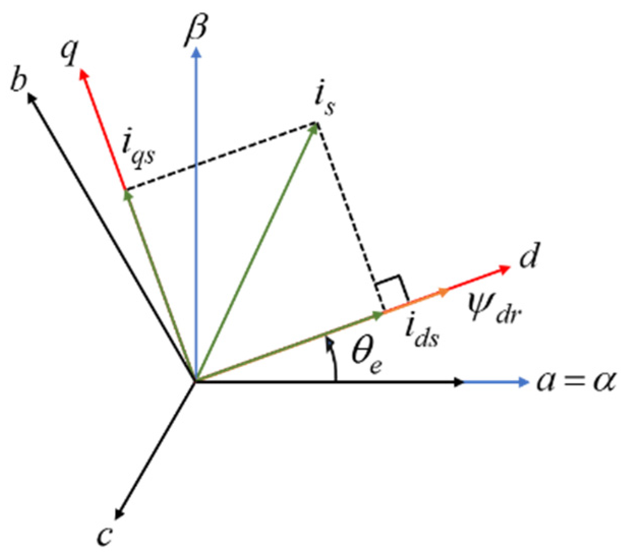
3. Indirect Field-Oriented Control

Indirect field-oriented control is a vector control with high acceptability in a high-performance drive system. The principle is essentially based on the decoupling between flux and torque through controlling the stator current component, as shown in Figure 2.

Based on the dynamic model of the IM, the three phase quantities are transformed into two coordinates on the d–q axes, which are the flux and torque components aligned on the q–axis and d–axis, respectively. To realize this condition, the rotor flux on the axis is set to be zero, while the d–axis reaches the nominal value of the magnetizing flux. The behavior of the drive system subjected to the rotor flux-oriented control is depicted in Figure 3.

With zero flux on the q–axis, the electromagnetic torque reduces to:

$${\tau }_e=\frac{3}{2}\left(\frac{p}{2}\right)\left(\frac{L_m}{L_r}\right)\left({\psi }_{dr}{}^e{i}_{qs}{}^e\right)$$

(3)

where p is the number of poles. The angular frequency of the rotor flux is given by:

$${\omega }_e={\omega }_r+{\omega }_{sl}$$

(4)

where the slip frequency is obtained from the q–axis stator current, such that:

$${\omega }_{sl}=\frac{L_m{i}_{qs}{}^e}{T_r{\psi }_{dr}{}^e}$$

(5)

The estimated rotor flux linkage can be calculated as:

$${\psi }_{dr}{}^e=\frac{L_m{i}_{ds}{}^e}{1+T_r\left(s\right)}$$

(6)

Thus, based on Equation (1), the angular position is given by:

$${\theta }_e={\theta }_r+{\displaystyle \underset{0}{\overset{t}{\int }}\left(\frac{L_m{i}_{qs}{}^e}{T_r{\psi }_{dr}{}^e}\right)}dt$$

(7)

From Figure 3, the use of a conventional voltage model’s (CVM) estimator could give a large back-EMF error, since the frequency and magnitude could be different in phase. By forming the suggested hybrid model given in the next section, the phase shift could be reduced by compensating for the back-EMF error in the CVM so that a nearly zero back-EMF error can be achieved.

4. Proposed Hybrid Flux and Speed Estimator with Speed Controller

The proposed model of the hybrid sensorless estimator is illustrated in Figure 4, where it works together with the conventional PI speed controller based on the virtual speed generation shown in Figure 3 in order to gain the minimum rotor speed error. The combination between the modified voltage model and the rotor flux-oriented current model was to give the least back-EMF error in estimating the rotor position of the IM. An adaptive PI control mechanism was added into the flux estimator of the back EMF for error generation. In this mode, the voltage model acted as the reference model, while the rotor flux-oriented current model acted as the adjustable model, to form a new model reference in this adaptive system topology. This system formed a hybrid and interacted with the speed estimator to estimate the rotor speed feedback being fed to the speed controller.

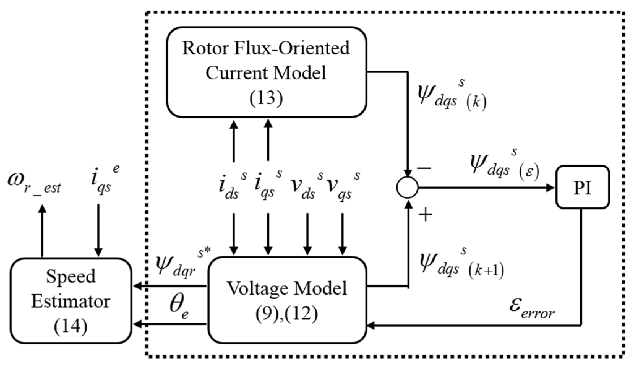
4.1. Sensorless Flux Estimator

The integration of the back EMF into the flux estimator was to estimate in advance the rotor flux with respect to the synchronously rotating frame for rotor position production. Two blocks, which were the voltage model and the rotor flux-oriented current model, were used to synthesize the rotor flux with respect to the stationary frame for the back-EMF error compensation. The plant was depicted as the flux estimator and can be expressed as:

$$S=M\left(i_{dqs}{}^s\right)+N\left({\psi }_{dqs}{{}^s}_{\left(k+1\right)}\right)$$

(8)

where $M=\sigma L_s$, $N=\frac{L_r}{L_m}$ and k = rotor flux at time k^th.

The stator flux is obtained by the stator reference current and voltage, such that:

$${\psi }_{dqs}{{}^s}_{\left(k+1\right)}={\displaystyle \underset{0}{\overset{t}{\int }}\left(v_{dqs}{}^s-R_s{i}_{dqs}{}^s-{\epsilon }_{emf}\right)}dt$$

(9)

The back-EMF error in Equation (9) is given as:

$${\epsilon }_{emf}=G\left({\psi }_{dqs}{{}^s}_{\left(\epsilon \right)}\right)$$

(10)

where G is a positive constant of proportional gain k_p and integral gain k_i. Thus, the adaptation mechanism law becomes:

$${\epsilon }_{emf}=k_p\left({\psi }_{dqs}{{}^s}_{\left(k+1\right)}-{\psi }_{dqs}{{}^s}_{\left(k\right)}\right)+k_i{\displaystyle \underset{0}{\overset{t}{\int }}\left({\psi }_{dqs}{{}^s}_{\left(k+1\right)}-{\psi }_{dqs}{{}^s}_{\left(k\right)}\right)}dt$$

(11)

The extraction of rotor flux from the stator flux is by using:

$${\psi }_{dqr}{}^{s*}=\frac{L_r}{L_m}\left({\psi }_{dqs}{{}^s}_{\left(k+1\right)}-\sigma L_s{i}_{dqs}{}^s\right)$$

(12)

As in the rotor flux-oriented current model, the stator flux is obtained by the stator current reference, and (6) can be expressed as:

$${\psi }_{dqs}{{}^s}_{\left(k\right)}=-M{i}_{dqs}{}^s+\frac{1}{N}{\left[{\left[i_{dqs}{}^s\right]}^T\left(\frac{L_m}{1+T_r\left(s\right)}\right)\right]}^{T-1}$$

(13)

where T and T⁻¹ are Park and inverse Park transformations, respectively. The stator flux in (13) acts as the feedback to the stator flux controller, which gives the compensated back-EMF error at a reduced level.

4.2. Sensorless Speed Estimator

The speed estimator in Figure 4 is another key building block of the proposed scheme. Angular frequency was used to determine the estimated speed. By subtracting slip frequency from angular frequency, as in Equation (4), the rotor speed can be determined. In the case of a pole machine, the slip speed as seen from the rotor frame ${\omega }_e-{\omega }_{r\_est}$ is equal to ${\omega }_e-\left(\frac{p}{2}\right){\omega }_{r\_est}$ and the rotor speed can be expressed as:

$${\omega }_{r\_est}=\frac{2}{p}\left(\frac{d{\theta }_e}{dt}-\frac{L_m{i}_{qs}{}^e}{T_r{\psi }_{dr}{}^e}\right)$$

(14)

The slip speed in (14) is taken into account to reduce the rotor losses in the air gap space. Through this consideration, the IM can give a high output of mechanical power. Thus, the efficiency of the IM is increased directly proportional to the input power.

5. Controller’s Stability on Proposed Hybrid Estimator for IFOC

In a conventional control method, a closed-loop system is where the output speed of the IM is fed back to the speed controller in order to obtain the transfer function. However, for this stability test, the closed-loop system used a current control, which was included for the transfer function derivation. Both stability analyses were tested when the new plant of the controllers was embedded with the hybrid estimator system for checking the new locations of the pole and zero.

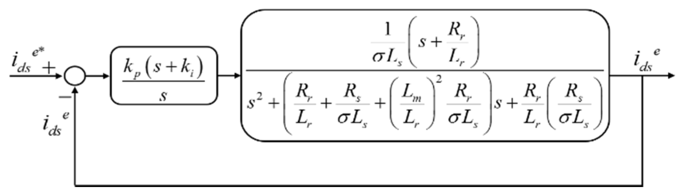
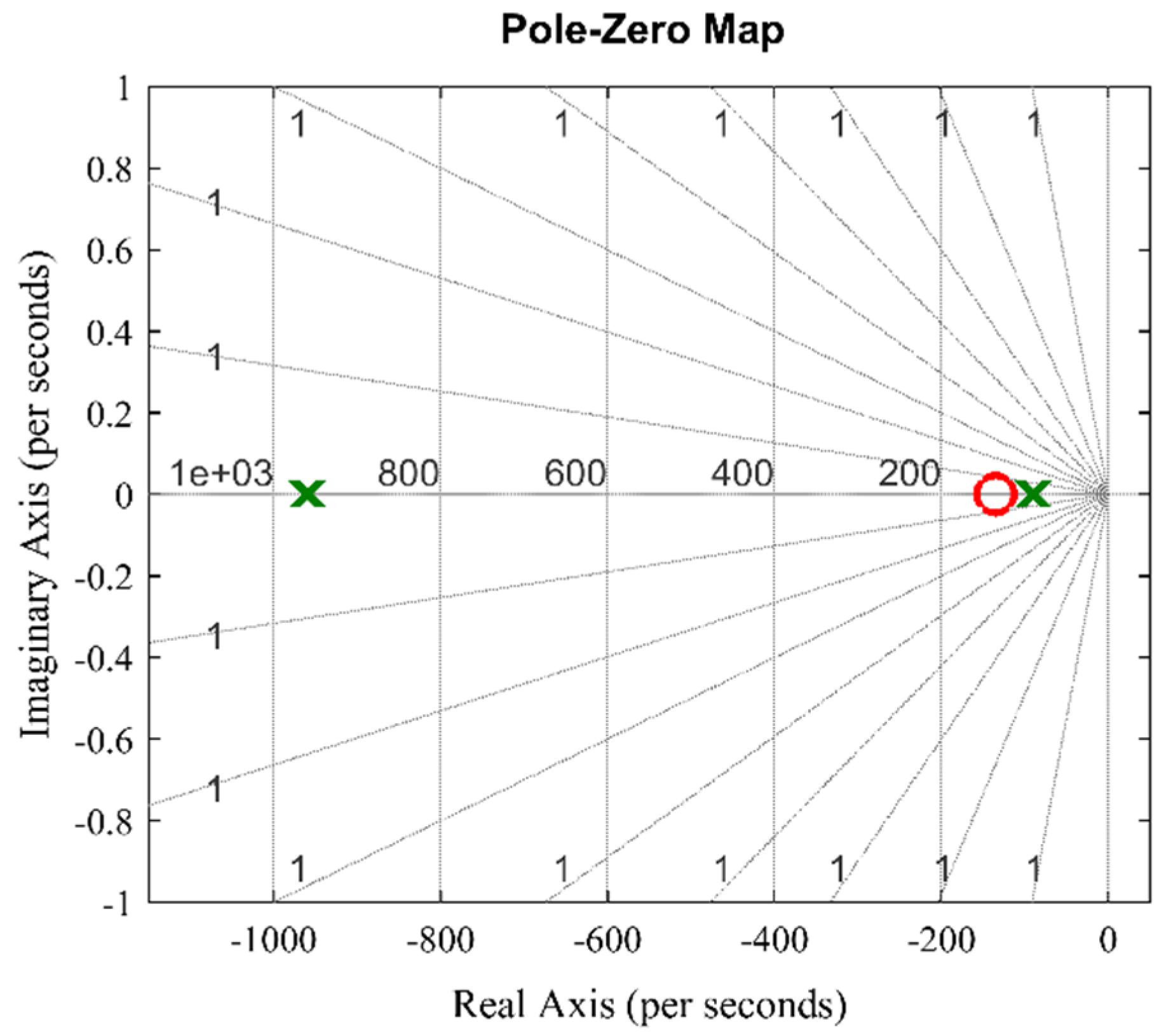
5.1. Inner Loop Current Control

It was important to ensure that the rotor flux remained constant so that a linear structure could be achieved. The inner loop of the plant system needed to be considered to fulfill the closed-loop transfer function. Therefore, the block diagram in Figure 5 was obtained after several calculations based on the IM circuit analysis with respect to the d–axis of the current controller.

A better understanding can be obtained based on Figure 6, where the closed-loop transfer function was interpreted into the pole-zero map plot. The closed-loop transfer function consisted of two poles, labeled as “X”, and one zero, labeled as “O”, that were plotted on the left-hand side of the pole-zero map. This validated that the closed-loop transfer function of the d–axis current controller was in a stable system.

The same implementation was also applied on the axis, where the slip was held at a value that ensured that the q–axis rotor flux was zero. The closed-loop transfer function for the axis current controller is shown in Figure 7.

The obtained closed-loop transfer function stability is shown in Figure 8. As observed, there were two poles and one zero on the left-hand side of the pole-zero map. This confirmed that the controller fulfilled the stability criterion, which meant that it was in a stable system.

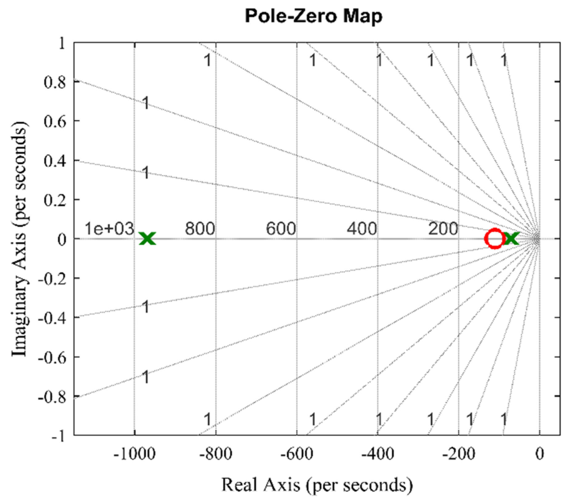
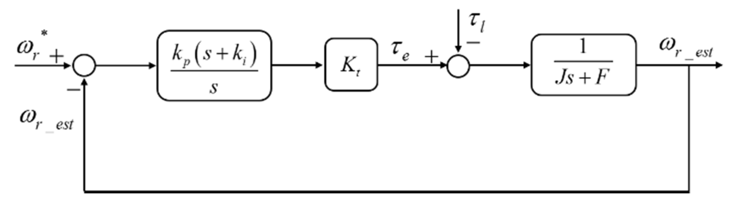
5.2. Outer Loop Speed Control

A current controller with a closed-loop time constant is ten times smaller than with a rotor or mechanical time constant. Under this condition, the current controller acts so rapidly that it can be neglected for practical purposes. The speed controller is designed based on a separately excited DC motor.

The control structure of the IM is shown in Figure 9 with the load torque, motor inertia and friction factors. All these parameters could affect the PI’s speed control response. Initially, the load torque was assumed to be zero. Therefore, the general closed-loop transfer function for the speed controller can be realized with the aid of the second-order system, as in [24], such that:

$$G\left(s\right)=\frac{{\omega }_n{}^2}{s^2+2\xi {\omega }_{n}s+{\omega }_n{}^2}$$

(15)

where ${\omega }_n$ is the natural frequency and ξ is the damping ratio. The overshoot percentage of the system is given as:

$$M_p=e^{\frac{\xi \pi }{\sqrt{1-{\xi }^2}}}$$

(16)

In order to have an overshoot between 2% and 5% of the speed response, the value of ξ and ${\omega }_n$ must be greater than 0.7 and 1.8 rad/s, respectively. Based on Equation (16), ξ can be calculated as:

$$\xi =-\frac{-\ln \left(M_p/100\right)}{\sqrt{{\pi }^2+{\ln }^2\left(M_p/100\right)}}$$

(17)

It can be defined that the settling is almost 98% of the final response value and the duration is approximately four times the time constant of the signal. When the time constant of the second-order control system is $1/\xi {\omega }_{rv}$, the steady-state settling time can be given as:

$$T_s=\frac{4}{\xi \omega }$$

(18)

Referring to the response of the closed-loop IM model under normal condition testing, the values of settling time and overshoot are 0.278 s and 0.025%, respectively. Substituting into (17), the value of ξ is 0.9352. Then, the value of ${\omega }_n$ is obtained based on (18) at 15.3861 rad/s.

Substituting the values of ξ and ${\omega }_n$ into (15), the general closed-loop transfer function for the speed controller can be expressed as:

$$G\left(s\right)=\frac{236.7321}{s^2+28.7782s+236.7321}$$

(19)

Based on the second-order closed-loop transfer function above, the stability of the system can be analyzed by solving the poles of the transfer function. It consists of two poles, labeled as “X”, which are −14.3891 + 5.4485i and −14.3891 − 5.4485i, with a negative real part and no positive pole, as shown in Figure 10.

6. Simulation Results

6.1. IM Performance under Parameter Variation

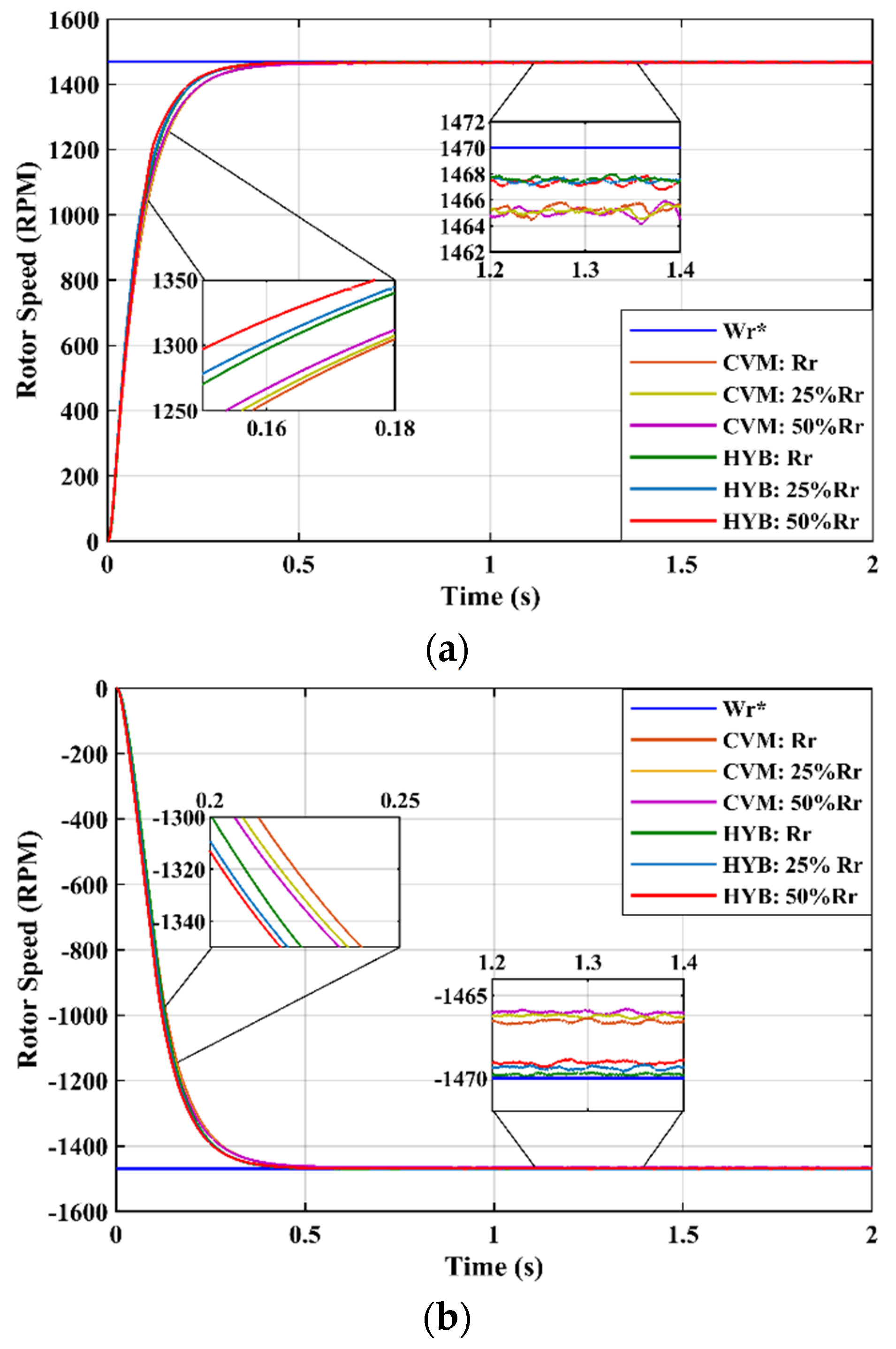
6.1.1. Rotor Resistance Variation

The block diagram of the estimator, depicted in Figure 4, consists of the stator flux control obtained from the rotor position by compensating the back-EMF error. Since rotor position is related to speed, which is affected by rotor time constant, it depends on rotor resistance, which varies according to temperature during the operation. To test the drive performance of the stator flux control in the suggested hybrid estimator, rotor resistance was varied by 50% of the nominal value with an increment of 25%. Figure 11a,b show the effect of rotor resistance variation on the rotor speed of two different estimators in two different modes. Both HYB and CVM estimators showed consistent performance in forward and reverse operations, with the results obtained confirming the estimator’s functions. The speed characteristics of the two estimators are summarized in

Table 1. Rotor speed performance under rotor resistance variation.

Mode	Step Info	Rotor Resistance Variation, Rr = 1.15 Ω
		Rr		25% Rr		50% Rr
		CVM	HYB	CVM	HYB	CVM	HYB
Forward	Settling time (s)	0.309	0.278	0.310	0.279	0.310	0.272
	Rise time (s)	0.169	0.152	0.168	0.151	0.166	0.143
	Overshoot (%)	0.035	0.025	0.038	0.022	0.048	0.038
	Speed error (rpm)	4.699	2.375	4.861	2.573	4.970	2.664
Reverse	Settling time (s)	0.343	0.319	0.343	0.317	0.342	0.316
	Rise time (s)	0.189	0.177	0.188	0.175	0.187	0.176
	Overshoot (%)	0.006	0.007	0.005	0.016	0.005	0.010
	Speed error (rpm)	3.448	2.760	3.752	0.652	4.007	0.957

. The two estimators without parameter uncertainty produced similar performances. However, compared with these two estimators, the conventional voltage model, which is not discussed here, took a longer time to track the reference rotor speed (blue line). When the hybrid estimator was applied, there was a shorter tracking time, but it was not remarkable.

Based on the rotor speed obtained for the proposed hybrid sensorless estimator, the stability response of the rotor flux against rotor resistance variation is shown in forward operation in Figure 12. As can be observed, the rotor flux response consisted of a few overshoots at the beginning due to the variation of 25% R_r and 50% R_r. However, the value was in an acceptable range of <20% overshoot with a 0.46 damping ratio. This confirms that the proposed hybrid estimation possesses a good dynamic response against parameter variation during its operation.

For more details,

Table 2. Rotor flux performance under rotor resistance variation.

Step Info	Rotor Resistance Variation, Rr = 1.15 Ω
	Rr	25% Rr	50% Rr
Settling time (s)	0.244	0.234	0.207
Rise time (s)	0.017	0.012	0.010
Peak value (Wb)	0.996	1.087	1.145
Overshoot (%)	3.336	12.858	19.032

summarizes the rotor flux response. It can be seen that the response is more superior without rotor resistance variation. Hence, with the proposed stator flux control as an adaptive mechanism, the response can be stable against rotor resistance variation with optimum overshoot and high capability of tracking rotor speed.

As recorded (Table 1), it can be concluded from the values of speed error that the hybrid estimator improved motor speed performance by compensating the back-EMF error into the CVM via controlling the stator flux of the IM. A minimum error was achieved with respect to reference speed with no oscillations.

6.1.2. Stator Resistance Variation

The voltage model consists of back-EMF error compensation, as in (9), and it is indicated that stator resistance variation should be taken into account in the study case. As mentioned above, the resistance varies due to temperature during motor operation. It could result in back-EMF error changes, consequently changing the speed’s estimated value. So, stator resistance was varied as with rotor resistance in Section 6.1.1 previously. As shown in Figure 13a,b, the speed estimation response operated at minimum error for both forward and reverse operations. The proposed estimator also gave excellent dynamic performance under stator resistance variation with a shorter time to track the reference rotor speed, as tabulated in

Table 3. Rotor speed performance under stator resistance variation.

Mode	Step Info	Rotor Resistance Variation, Rs = 0.6 Ω
		Rs		25% Rs		50% Rs
		CVM	HYB	CVM	HYB	CVM	HYB
Forward	Settling time (s)	0.309	0.278	0.304	0.275	0.300	0.270
	Rise time (s)	0.169	0.152	0.167	0.150	0.164	0.146
	Overshoot (%)	0.035	0.025	0.029	0.005	0.010	0.013
	Speed error (rpm)	4.699	2.375	4.678	2.327	4.656	2.282
Reverse	Settling time (s)	0.343	0.319	0.342	0.316	0.339	0.313
	Rise time (s)	0.189	0.177	0.187	0.175	0.185	0.173
	Overshoot (%)	0.006	0.007	0.005	0.017	0.003	0.011
	Speed error (rpm)	3.448	2.760	3.376	0.186	3.312	0.109

. Clearly, the speed estimation efficiently tracked the reference with a speed error range of below 10 rpm and an acceptable range of <20% overshoot. Stator resistance variation had the least effect on IM response compared with rotor resistance variation due to the exact amount of back-EMF error compensation by the adaptation mechanism of stator flux control at the stator side.

6.1.3. Mutual Inductance Variation

When involving temperature, the mutual inductance parameter was also taken into account in this study case. The values of stator and rotor inductance parameters in this research were the same. The variation in inductance also affect the mutual inductance of the IM. Several studies on inductance against temperature have been conducted, such as in [25], which concluded that inductance remains functional in a high temperature and there is no temperature dependence. However, [26] stated that a 1% change in resistance produced by 2.54 °C corresponds to a 0.0076% increase in inductance. In this research, mutual inductance was varied by 25% and 50% of the nominal value. This means that the temperature was very high during motor operation. As shown in Figure 14a,b, the effect of mutual inductance gave almost the same speed response in both forward and reverse operations either for the CVM or the HYB. Referring to

Table 4. Rotor speed performance under mutual inductance variation.

Mode	Step Info	Rotor Resistance Variation, Lm = 18.82 mH
		Lm		25% Lm		50% Lm
		CVM	HYB	CVM	HYB	CVM	HYB
Forward	Settling time (s)	0.309	0.279	0.310	0.280	0.308	0.278
	Rise time (s)	0.169	0.152	0.169	0.152	0.168	0.151
	Overshoot (%)	0.016	0.037	0.018	0.002	0.070	0.033
	Speed error (rpm)	4.693	2.374	4.641	2.362	4.662	2.337
Reverse	Settling time (s)	0.344	0.318	0.342	0.316	0.344	0.318
	Rise time (s)	0.189	0.178	0.188	0.176	0.188	0.176
	Overshoot (%)	0.014	0.025	0.030	0.056	0.029	0.042
	Speed error (rpm)	3.448	0.277	3.452	0.315	3.457	0.358

, the HYB estimator could improve the dynamic performance of the IM compared with the CVM, as the average speed error was below 0.16%. This proves that the proposed estimator works effectively against parameter variation.

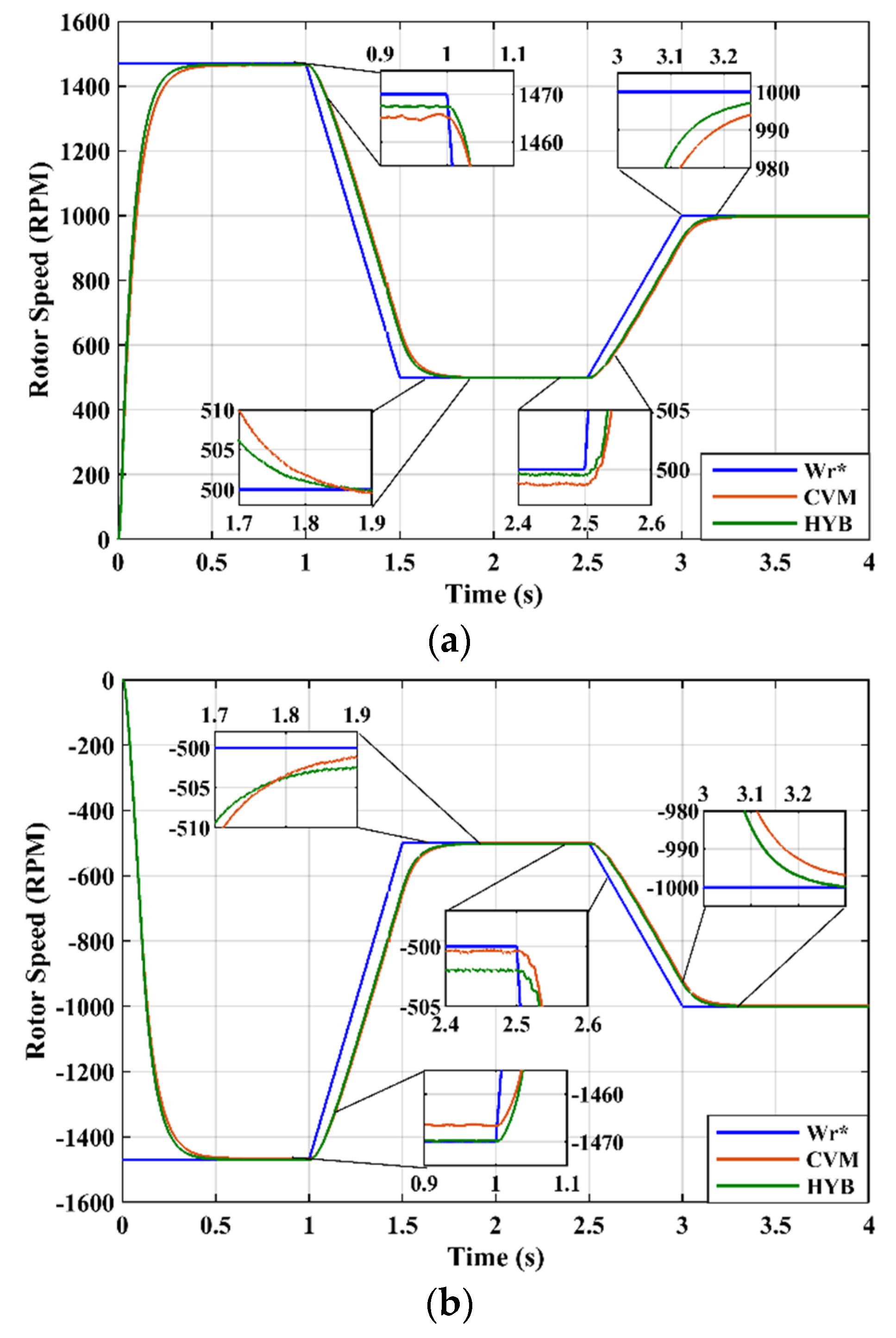
6.2. IM Performance under Variable Speed Trajectory

The derivative of rotor position with time was then applied to determine the rotor speed during driving, since the feedback of the speed estimator to the reference speed determines the speed error of the control system. Figure 15a,b show the speed tracking response with respect to the speed reference in order to seek the speed tracking capability. The reference speed was given in the trapezoidal signal input with a constant value during the motor’s starting operation in order to see the transient behavior. The variable speed trajectory was applied in forward and reverse motoring operations with the proposed hybrid estimator of the stator flux control.

Using accurate rotor position tracking, the speed error was minimized nearly to zero. A good tracking capability was obtained in both reverse and forward operations with no overshoots at the starting of the IM. As can be seen between 1.5 and 3 s, the speed errors were recorded in

Table 5. Rotor speed performance under variable speed trajectory.

Mode	Step Info	Rotor Speed Variation (rpm)
		500 rpm		1000 rpm
		CVM	HYB	CVM	HYB
Forward	Time lag (s)	0.544	0.480	0.533	0.447
	Speed error (rpm)	1.215	0.408	2.851	1.323
Reverse	Time lag (s)	0.527	0.476	0.530	0.397
	Speed error (rpm)	0.421	2.047	1.550	0.678

from the reference values at 0.082% and 0.132%, respectively. Meanwhile, in the existing voltage model estimator, it contributed about 0.243% and 0.285% errors for both speed trajectories. With the 0.161% and 0.153% margin errors, the hybrid estimator has shown an excellent performance in estimating speeds using the stator flux control under a variable speed trajectory. This shows that the back-EMF error was completely compensated into the voltage model in order to create the correct position of the rotor.

The stability of the speed controller’s response can be seen in Figure 16a–c, which present the forward motoring operation. In Figure 16a, the spiral graph shows a highly stable response during full-speed operation without any ripples. Meanwhile, as shown in Figure 16b, at a minimum low speed of 500 rpm, the current faced a few ripples with a stable response. This happened due to the integration of very small signals of angular frequency that made the rotor position shifted a few degrees. When reaching 1000 rpm, as shown in Figure 16c, the spiral response of the current had fewer ripples compared with the response at a lower speed. However, the speed estimation response was within the boundary of the speed reference’s range and a high speed-tracking capability was obtained with accurate rotor position estimation.

6.3. IM Performance at Very Low Speed under Regenerative Braking and Zero-Speed Conditions

In order to behave like in a real EV operation, the four-quadrant operation needed to be fulfilled. In the above section, forward and reverse motoring had been discussed, and is not repeated here. Forward braking and reverse braking are under the regenerative mode and could be realized by slowing down the reference speed or applying a mechanical load to the IM to reduce the speed to 0 rpm. In this research, a mechanical load was applied at τ = 20 Nm to show the IM braking and operating at a very low speed. In addition, a mechanical load was also applied at τ = 40 Nm to show the IM braking until the steady-state zero-speed condition. Figure 17a,b show the response of braking in two different operations. As can be seen, the IM operated at a very low speed by following the reference speed at 100 rpm. At time τ = 1.5 s, a mechanical load was applied to show the braking system slowing down the IM until the extra-low speed of 50 rpm and zero-speed condition at 0 rpm. As shown in

Table 6. Rotor speed performance at very low speed in regenerative braking.

Mode	Step Info	Reference Low Speed, ωr = 100 rpm
		τm = 20 Nm		τm = 40 Nm
		CVM	HYB	CVM	HYB
Forward braking	Settling time (s)	1.236	1.193	1.279	1.115
	Rise time (s)	0.163	0.136	0.187	0.159
	Overshoot (%)	1.334	1.652	2.000	2.518
	Speed error (rpm)	0.750	0.741	1.269	0.925
Reverse braking	Settling time (s)	1.231	1.218	1.258	1.215
	Rise time (s)	0.164	0.138	0.168	0.142
	Overshoot (%)	1.135	0.811	0.505	0.837
	Speed error (rpm)	0.751	0.728	0.767	0.750

, the speed error obtained was less than 1 rpm for the proposed HYB estimator compared with the speed error for the CVM, which was more than 1 rpm at zero speed. This shows that the speed tracking capability successfully reduced speed estimation errors. This confirms that the proposed HYB is able to improve speed tracking capability and operate the IM under very-low-speed conditions.

This also indicates that the HYB estimator was able to operate under zero-speed conditions, where its speed estimation had the least mismatch compared with the CVM in tracking the actual zero speed. Figure 18 shows the speed estimation by the HYB, as well as the speed estimation error of under 2 rpm, approaching zero with accurate flux estimation. Furthermore, the results confirmed that the rotor flux position was at accurate reference speed, while not losing stability in very-low-speed operation. This satisfies the supremacy of the HYB’s flux estimation in extracting accurate speed estimation under very-low-speed and zero-speed conditions.

6.4. IM Performance under Load Torque Disturbances

Since speed and torque are related to each other, a justification can be made under the load torque disturbances, as presented in Figure 19a and 19b for the forward and reverse operations, respectively, that torque does not give any effect to the controller. Torque disturbances were set up at times t = 0.7 s, 1.3 s and 2 s with torque values of 50 Nm, 75 Nm and 100 Nm, respectively. As depicted in Figure 19, there was a quick convergence in the speed response after the load disturbances were rejected. The quality of estimation also can be seen in the speed errors, which were relatively low as expected. The speed estimation response tracked the constant reference speed in spite of load torque disturbances both in forward and reverse operations. In addition, the dynamics of the IM was still maintained with no overshoots and oscillations during the starting of the IM.

Table 7. Rotor speed performance under load torque disturbances.

Mode	Step Info	Load Torque Disturbances (Nm)
		50 Nm		75 Nm		100 Nm
		CVM	HYB	CVM	HYB	CVM	HYB
Forward	Time lag (s)	0.436	0.357	0.405	0.328	0.394	0.315
	Speed error (rpm)	42	38	60	56	77	73
Reverse	Time lag (s)	0.417	0.333	0.386	0.325	0.357	0.323
	Speed error (rpm)	40	36	58	54	76	72

shows the summary of the torque load effect on the two estimators. Clearly, there were smaller speed drops in the hybrid (HYB) estimator compared with the CVM due to the compensated EMF error that changed the stator flux response. A faster recovery time was noticed in the proposed HYB estimator with an average of 0.078 s, which gave the IM an excellent performance. Additionally, there were no ripples on the speed response, which meant that the IM did not suffer from torque cogging.

7. Performance Evaluation Comparison

Based on the presented simulation result, the good dynamic performance of the IM was successfully achieved by the suggested model. The HYB estimator was effectively more robust than the CVM. The results demonstrate that the system exhibits good speed estimation accuracy under different conditions. This is supported by the stability effect given in Figure 16 for speed and current controllers, which are responsible for controlling the torque and speed of the IM. An evaluation table (

Table 8. Comparison table of FOC scheme with different estimation methods.

Authors	[28,29]	[30,31,32]	[33,34]	[35,36]	Proposed
Type of FOC	Sensorless IFOC	Sensorless IFOC	Sensorless DFOC	Sensorless IFOC	Sensorless IFOC
Control variable	V & I	I & Wr	V & I	V & I	I, Wr & EMF
Inverter control	PWM	SV-PWM	PWM	SV-PWM	SV-PWM
Speed control	Fuzzy	PI	PI	PI	PI
Estimation method	V & I model	Fictitious resistance based on V & I model	Reactive power based on V & I model	EMF based on V & I model	EMF compensation based on V & rotor flux-oriented I model
Complexity	MED	MED	HI	MED	MED
* Average speed error (%)	LS: 26.67 HS: 33.00	Constant LS: 1.00	Conventional: 0.20 (Act) 2.30 (Est) Proposed: 0.10 (Act) 0.40 (Est)	LS: 0.50	Conventional (Est): LS: 0.24 (F), 0.08 (R) HS: 0.32 (F), 0.24 (R) Proposed (Est): LS: 0.08 (F), 0.40 (R) HS: 0.16 (F), 0.06 (R)

Notes: * calculated from measured and reference value. V, voltage; I, current; Wr, rotor speed; EMF, electromotive force; LS, low speed; HS, high speed; F; forward; R, reverse; PI, proportional integral; SV-PWM, space vector pulse width modulation; MED, medium; HI, high; Est, estimated; Act, actual.

) is provided to compare with the findings from previous research works, as examined in [27], to clarify the improvements that have been achieved with the suggested model.

8. Conclusions

This paper presents a hybrid estimator model, along with the accuracy analysis of speed and torque tracking of an IFOC in estimating rotor flux position and speed to control the speed of the IM. The parameters of the IM are listed in the Appendix A,

Table A1. Parameters of induction motor.

Parameter	Value
DC voltage	800 V
Inverter frequency	5 kHz
Rated power	20 hp
Rated speed	1500 rpm
Rated voltage	400 V
Frequency	50 Hz
Stator resistance	0.6 Ω
Rotor resistance	1.15 Ω
Stator inductance	19.561 mH
Rotor inductance	19.561 mH
Magnetizing inductance	18.82 mH
Inertia	0.2 kg.m2
Number of pole pairs	2

. In order to enhance speed control, a new model of hybrid estimator was proposed with stator flux control as the adaptation mechanism. The proposed estimator was investigated under four cases: (1) parameter sensitivity against rotor and stator resistance and mutual inductance variation, (2) variable speed trajectory, (3) very low speed in regenerative mode and zero-speed conditions and (4) variable load torque disturbances. The analyses showed that the three controllers were confirmed in a stable operation, as evidenced by the pole-zero maps.

All results proved that parameter sensitivity did not affect speed response. All speed responses also showed good tracking capability under variable speed trajectories and had faster recovery time under torque disturbances by using the hybrid estimator as compared with the conventional model. The proposed control scheme was successfully validated in various cases. The stability analysis and reported results showed excellent performance of the IM in both forward and reverse operations at a steady state and during transients.

References

1. Quintero-Manriquez, E.; Sanchez, E.N.; Felix, R.A. Real-time direct field-oriented and second order sliding mode controllers of induction motor for electric vehicles applications. In Proceedings of the 2015 10th System of Systems Engineering Conference (SoSE), San Antonio, TX, USA, 17–20 May 2015; pp. 220–225. [Google Scholar] [CrossRef]
2. Chan, C.C. The Rise & Fall of Electric Vehicles in 1828–1930: Lessons Learned [Scanning Our Past]. Proc. IEEE 2013, 101, 206–212. [Google Scholar] [CrossRef] [Green Version]
3. Olarescu, N.-V.; Weinmann, M.; Zeh, S.; Musuroi, S.; Sorandaru, C. Optimum torque control algorithm for wide speed range and four quadrant operation of stator flux oriented induction machine drive without regenerative unit. In Proceedings of the 2011 IEEE Energy Conversion Congress and Exposition, Phoenix, AZ, USA, 17–22 September 2011; pp. 1773–1777. [Google Scholar] [CrossRef]
4. Odhano, S.A.; Bojoi, R.; Boglietti, A.; Rosu, S.G.; Griva, G. Maximum Efficiency per Torque Direct Flux Vector Control of Induction Motor Drives. IEEE Trans. Ind. Appl. 2015, 51, 4415–4424. [Google Scholar] [CrossRef]
5. Paulus, D.; Stumper, J.-F.; Kennel, R. Sensorless Control of Synchronous Machines Based on Direct Speed and Position Estimation in Polar Stator-Current Coordinates. IEEE Trans. Power Electron. 2013, 28, 2503–2513. [Google Scholar] [CrossRef]
6. Liu, K.; Zhu, Z.Q.; Stone, D.A. Parameter Estimation for Condition Monitoring of PMSM Stator Winding and Rotor Permanent Magnets. IEEE Trans. Ind. Electron. 2013, 60, 5902–5913. [Google Scholar] [CrossRef] [Green Version]
7. Kandoussi, Z.; Boulghasoul, Z.; Elbacha, A.; Tajer, A. Fuzzy sliding mode observer based sensorless Indirect FOC for IM drives. In Proceedings of the 2015 Third World Conference on Complex Systems (WCCS), Marrakech, Morocco, 23–25 November 2015; pp. 1–6. [Google Scholar] [CrossRef]
8. Alonge, F.; D’Ippolito, F.; Sferlazza, A. Sensorless Control of Induction-Motor Drive Based on Robust Kalman Filter and Adaptive Speed Estimation. IEEE Trans. Ind. Electron. 2014, 61, 1444–1453. [Google Scholar] [CrossRef]
9. Harnefors, L.; Saarakkala, S.E.; Hinkkanen, M. Speed Control of Electrical Drives Using Classical Control Methods. IEEE Trans. Ind. Appl. 2013, 49, 889–898. [Google Scholar] [CrossRef]
10. Sun, X.; Yi, Y.; Zheng, W.; Zhang, T. Robust PI speed tracking control for PMSM system based on convex optimization algorithm. In Proceedings of the 33rd Chinese Control Conference, Nanjing, China, 28–30 July 2014; pp. 4294–4299. [Google Scholar] [CrossRef]
11. Zaky, M.S. A stable adaptive flux observer for a very low speed-sensorless induction motor drives insensitive to stator resistance variations. Ain Shams Eng. J. 2011, 2, 11–20. [Google Scholar] [CrossRef] [Green Version]
12. Alsofyani, I.M.; Idris, N. A review on sensorless techniques for sustainable reliablity and efficient variable frequency drives of induction motors. Renew. Sustain. Energy Rev. 2013, 24, 111–121. [Google Scholar] [CrossRef]
13. Li, C.; Chen, M.; Gao, S. Fractional order PI speed control for permanent magnet synchronous motor drives. In Proceedings of the 11th World Congress on Intelligent Control and Automation, Shenyang, China, 29 June–4 July 2014; pp. 4681–4685. [Google Scholar]
14. Sariyildiz, E.; Yu, H.; Ohnishi, K. A Practical Tuning Method for the Robust PID Controller with Velocity Feed-Back. Machines 2015, 3, 208–222. [Google Scholar] [CrossRef] [Green Version]
15. Zemmit, A.; Messalti, S.; Harrag, A. A new improved DTC of doubly fed induction machine using GA-based PI controller. Ain Shams Eng. J. 2018, 9, 1877–1885. [Google Scholar] [CrossRef]
16. Mora, A.; Orellana, A.; Juliet, J.; Cardenas, R. Model Predictive Torque Control for Torque Ripple Compensation in Variable-Speed PMSMs. IEEE Trans. Ind. Electron. 2016, 63, 4584–4592. [Google Scholar] [CrossRef]
17. Zhou, Y.; Shang, W.; Liu, M.; Li, X.; Zeng, Y. Simulation of PMSM vector control based on a self-tuning fuzzy PI controller. In Proceedings of the 2015 8th International Conference on Biomedical Engineering and Informatics (BMEI), Shenyang, China, 14–16 October 2015; pp. 609–613. [Google Scholar] [CrossRef]
18. Saleem, O.; Omer, U. EKF-based self-regulation of an adaptive nonlinear PI speed controller for a DC motor. Turk. J. Electr. Eng. Comput. Sci. 2017, 25, 4131–4141. [Google Scholar] [CrossRef]
19. Lftisi, F.; George, G.; Aktaibi, A.; Butt, C.; Rahman, M.A. Artificial neural network based speed controller for induction motors. In Proceedings of the IECON 2016–42nd Annual Conference of the IEEE Industrial Electronics Society, Florence, Italy, 23–26 October 2016; pp. 2708–2713. [Google Scholar] [CrossRef]
20. Hasan, A.; Mishra, R.K.; Singh, S. Speed Control of DC Motor Using Adaptive Neuro Fuzzy Inference System Based PID Controller. In Proceedings of the 2019 2nd International Conference on Power Energy, Environment and Intelligent Control (PEEIC), Greater Noida, India, 18–19 October 2019; pp. 138–143. [Google Scholar] [CrossRef]
21. Areed, F.G.; Haikal, A.Y.; Mohammed, R.H. Adaptive neuro-fuzzy control of an induction motor. Ain Shams Eng. J. 2010, 1, 71–78. [Google Scholar] [CrossRef]
22. Zolfaghari, M.; Taher, S.A.; Munuz, D.V. Neural network-based sensorless direct power control of permanent magnet synchronous motor. Ain Shams Eng. J. 2016, 7, 729–740. [Google Scholar] [CrossRef] [Green Version]
23. Sepeeh, M.S.; Zulkifli, S.A.; Sim, S.Y.; Pathan, E. A Comprehensive Review of Field-Oriented Control in Sensorless Control Techniques for Electric Vehicle. Int. Rev. Electr. Eng. (IREE) 2018, 13, 461–475. [Google Scholar] [CrossRef]
24. Farah, N.; Talib, M.H.N.; Shah, N.S.M.; Abdullah, Q.; Ibrahim, Z.; Lazi, J.B.M.; Jidin, A. A Novel Self-Tuning Fuzzy Logic Controller Based Induction Motor Drive System: An Experimental Approach. IEEE Access 2019, 7, 68172–68184. [Google Scholar] [CrossRef]
25. Doumit, N.; Danoumbé, B.; Capraro, S.; Chatelon, J.-P.; Blanc-Mignon, M.-F.; Rousseau, J.-J. Temperature impact on inductance and resistance values of a coreless inductor (Cu/Al2O3). Microelectron. Reliab. 2017, 72, 30–33. [Google Scholar] [CrossRef]
26. Satish, S.; Ansari, M.A.; Saxena, A.K. Determination and comparison of temperature coefficients of standard inductors using different methods. In Proceedings of the 2012 Conference on Precision electromagnetic Measurements, Washington, DC, USA, 1–6 July 2012; pp. 404–405. [Google Scholar] [CrossRef]
27. Sepeeh, M.S.; Zulkifli, S.A.; Sim, S.Y. A Simulation on Hybrid Speed and Flux Estimation-Based Back EMF Integration with Rotor Flux-Oriented Current Model. Int. Rev. Model. Simul. (IREMOS) 2020, 13, 97–107. [Google Scholar] [CrossRef]
28. Orlowska-Kowalska, T.; Dybkowski, M. Stator-Current-Based MRAS Estimator for a Wide Range Speed-Sensorless Induction-Motor Drive. IEEE Trans. Ind. Electron. 2010, 57, 1296–1308. [Google Scholar] [CrossRef]
29. Wang, G.; Xu, D.; Yu, Y.; Chen, W. Improved rotor flux estimation based on voltage model for sensorless field-oriented controlled induction motor drives. In Proceedings of the 2008 IEEE Power Electronics Specialists Conference, Rhodes, Greece, 15–19 June 2008; pp. 1887–1890. [Google Scholar] [CrossRef]
30. Krishna, S.M.; Daya, J.F. MRAS speed estimator with fuzzy and PI stator resistance adaptation for sensorless induction motor drives using RT-lab. Perspect. Sci. 2016, 8, 121–126. [Google Scholar] [CrossRef] [Green Version]
31. Farasat, M.; Trzynadlowski, A.M.; Fadali, M.S. Efficiency improved sensorless control scheme for electric vehicle induction motors. IET Electr. Syst. Transp. 2014, 4, 122–131. [Google Scholar] [CrossRef]
32. Pal, A.; Kumar, R.; Das, S. Sensorless Speed Control of Induction Motor Driven Electric Vehicle Using Model Reference Adaptive Controller. In Proceedings of the Energy Procedia 5th International Conference on Advances in Energy Research, (ICAER 2015), Mumbai, India, 15–17 December 2015; pp. 540–551. [Google Scholar] [CrossRef]
33. Ta, C.-M.; Uchida, T.; Hori, Y. MRAS-based speed sensorless control for induction motor drives using instantaneous reactive power. In Proceedings of the 27th Annual Conference of the IEEE Industrial Electronics Society (IECON’01), Denver, CO, USA, 29 November–2 December 2001; pp. 1417–1422. [Google Scholar] [CrossRef]
34. Yujie, L.; Shaozhong, C. Model reference adaptive control system simulation of permanent magnet synchronous motor. In Proceedings of the 2015 IEEE Advanced Information Technology, Electronic and Automation Control Conference (IAEAC), Chongqing, China, 19–20 December 2015; pp. 498–502. [Google Scholar] [CrossRef]
35. Zhifu, W.; Jun, F.; Zhijian, S.; Qiang, S. Study on Speed Sensor-less Vector Control of Induction Motors Based on AMEsim-Matlab/Simulink Simulation. In Proceedings of the 8th International Conference on Applied Energy (ICAE2016), Beijing, China, 8–11 October 2016; pp. 2378–2383. [Google Scholar] [CrossRef]
36. Bensiali, N.; Etien, E.; Benalia, N. Convergence analysis of back-EMF MRAS observers used in sensorless control of induction motor drives. Math. Comput. Simul. 2015, 115, 12–23. [Google Scholar] [CrossRef]
Figure 1. Space vector of ideal three-phase induction motor.
Machines 10 01089 g001
Figure 2. Phasor diagram of FOC’s drive system.
Machines 10 01089 g002
Figure 3. Indirect field-oriented control of IM.
Machines 10 01089 g003
Figure 4. Block diagram of flux and speed estimator.
Machines 10 01089 g004
Figure 5. Simplified block diagram of d–axis current controller.
Machines 10 01089 g005
Figure 6. Pole-zero plot of closed-loop transfer function of d–axis current controller.
Machines 10 01089 g006
Figure 7. Simplified block diagram of q–axis current controller.
Machines 10 01089 g007
Figure 8. Pole-zero plot of closed-loop transfer function of q–axis current controller.
Machines 10 01089 g008
Figure 9. Simplified block diagram of speed controller.
Machines 10 01089 g009
Figure 10. Pole-zero plot of closed-loop transfer function of speed controller.
Machines 10 01089 g010
Figure 11. Rotor speed response against rotor resistance variation: (a) in forward operation and (b) in reverse operation.
Machines 10 01089 g011
Figure 12. Alpha-beta rotor flux response against rotor resistance variation.
Machines 10 01089 g012
Figure 13. Rotor speed response against stator resistance variation: (a) in forward operation and (b) in reverse operation.
Machines 10 01089 g013
Figure 14. Rotor speed response against mutual inductance variation: (a) in forward operation and (b) in reverse operation.
Machines 10 01089 g014
Figure 15. Rotor speed response under variable speed trajectory: (a) in forward operation and (b) in reverse operation.
Machines 10 01089 g015
Figure 16. Alpha-beta stator current response: (a) at 1470 rpm, (b) at 500 rpm and (c) at 1000 rpm.
Machines 10 01089 g016
Figure 17. Rotor speed response at very low speed in regenerative braking: (a) in forward operation and (b) in reverse operation.
Machines 10 01089 g017
Figure 18. Rotor speed response at zero speed condition.
Machines 10 01089 g018
Figure 19. Rotor speed response under load torque disturbances: (a) in forward operation and (b) in reverse operation.
Machines 10 01089 g019