Calibration Method for In-Process Identification of Tangential Specific Cutting Force in Milling

Abstract

The cutting forces that occur during machining cause static and dynamic deformations of the machine–tool–workpiece system. In general, the cutting force is spatial. However, knowledge of the tangential component of the cutting force is crucial for the optimum use of the power installed on the spindle. An important parameter for cutting force modeling is the tangential cutting force coefficient. This paper focuses on the approach of the in-process identification of the cutting and edge components of the tangential cutting force coefficient, using the spindle power signal read directly from the machine tool control system. Such procedures have already been described in the available literature. The key point for the successful implementation of these methods is the identification and avoidance of the passive torque signal. This paper describes the operational calibration of the spindle drive system. The calibration procedure is based on the tap test using modal hammer excitation and the spindle power signal response. The proposed procedure was successfully validated using a machine–machine comparison approach and a machine–dynamometer validation approach. The results are consistent with those in the available literature. With this method, we were able to determine the cutting component of the tangential specific cutting force with a deviation of 1% from the reference system and an edge component of 10%. The modal hammer method only enables the avoidance of dynamometers in the machine calibration procedure.

1. Introduction

The cutting forces that occur during machining cause static and dynamic deflections of the machine–tool–workpiece system. Workpiece out-of-tolerance dimensions and poor surface quality may result from the process–machine interaction. Thus, it is important to be able to define the cutting force size before or during the machining process.

The milling cutting force is spatial with three main components: tangential, radial, and axial components, described in the rotating coordinate system of the tool. Although all of the force components are important for the prediction of machining quality, the tangential component is of greater importance as the “torque-building” component. The tangential cutting force component is the key component for spindle power estimation.

There are two types of cutting force models that are widely used. The Kienzle model [1] defines the cutting force as proportional to the varying chip thickness and the constant value of a specific cutting force. The specific cutting force is a constant value depending on the workpiece material, cutting-edge geometry (including that the cutting-edge geometry changes due to tool wear), cutting conditions, and type of cooling. Despite the mentioned multiple value limits, the specific cutting force has been widely used in industries for the predictive estimation of cutting forces; see, e.g., the SANDVIK Coromant website [2] or MDoctor website [3]. This model was also incorporated into the first machining stability models [4] as a simple and useful cutting force model.

The Kienzle model predicts an almost zero force for almost zero chip thickness. This is not a realistic estimation due to the rubbing effects between the cutting-edge and workpiece material. Fu [5] and, later, Spiewak [6] introduced a mechanistic cutting force model. The sizes of all three of the main cutting force components are described with two specific components: the edge component characterizes the cutting force share related to the cutting-edge friction on the machined surface, and the cutting component share is related to the undeformed chip thickness. This means that the special cutting force size can be described using six constant cutting force coefficients for a specific combination of the workpiece material and cutting-edge geometry.

All six cutting force coefficients can be identified using experiments based on cutting force measurements with a dynamometer for the multiple feed per tooth values [5]. This implies a large volume of experimental work. Budak [7] proposed a method where basic cutting force coefficients are identified during orthogonal machining. For other engagement situations, orthogonal to oblique transformation is used. If a stationary dynamometer is used in the experiment, the tangential cutting force cannot be read directly. Then, during the milling process, it is necessary to clamp only one cutting insert and calculate the tangential component from the active component, as presented by Kovalcik [8].

An alternative approach for tangential cutting force coefficients that does not require a special dynamometer is based on spindle power monitoring and known tool engagement conditions. This can be performed with special instruments; see Qiu in [9]. Qiu performed his experiments in turning. This presents the possibility of measuring the spindle power or torque with such a tool and saving on expensive equipment. All main control system manufacturers integrate the ability to measure information about the controlled axes into their products: the Servo trace (Sinumerik), the TNCscope (HEIDENHAIN), and the Servo Guide (Fanuc). With spindle power monitoring for the specific cutting force identification, it is critical to identify the passive torque of the spindle before the measured data are evaluated. Dunwoody [10] and Aggarwal [11] presented the identification of passive spindle current models at various levels of detail and the subsequent implementation for the identification of the tangential cutting force coefficients. Janota showed that it is possible to identify specific cutting force coefficients by taking control system measurements, in [12]. Recent developments include the use of a digital twin (see Caesar in [13]) and the identification of all cutting force components by machine tool measurements (see Liu in [14]). The latter approach aims to determine tool wear from the contribution of the tangential and normal cutting force components.

A fundamental prerequisite for the credibility of the results of any experiment is the comparison of the measurement chain with the standard. This type of comparison is called calibration. Most of the authors used a linear or rotary piezoelectric dynamometer to verify their methods. One example is Yamato’s calibration [15] of the output of a control system over the entire frequency range. He proposed a two-step procedure to identify the cutting forces. He first took measurements with a dynamometer, corrected his cutting force model, and then machined without a dynamometer.

However, verification using a dynamometer is not always possible. The additional mass of the clamped workpiece and the compliance of the dynamometer reduce the useful frequency range of the measurement. Rotary dynamometers only allow the clamping of the tools up to a certain diameter, and their compliance reduces the stability limit and thus limits the range of applicable cutting conditions. An apparatus incorporating a dynamometer is also less mobile and requires multiple channel connections.

One of the sensors commonly used in dynamic measurements is the modal hammer. A modal hammer is a special hammer with a built-in force gauge. It is, therefore, used for both excitation and impulse force measurements. For the required calibration of the machine tool signal, the modal hammer may be used as a force standard. Performing a calibration before each measurement is a prerequisite for suppressing systematic measurement errors.

This article focuses on the calibration of the measurement of the chain cutting process–machine tool spindle using modal hammer excitation on the tool and the measurement of the spindle drive response. The main motivation behind this approach is the flexible operational usage of the modal hammer to avoid the need for the complicated installation of the dynamometer. The article is structured as follows: In Section 2, a calibration method is proposed. In Section 3, the proposed procedure is verified using two validation approaches: a machine-to-dynamometer experiment and a machine-to-machine comparison. In Section 4, the results are discussed, and the limits of the method are commented on. The paper concludes with Section 5.

2. Description of the Calibration Method Approach

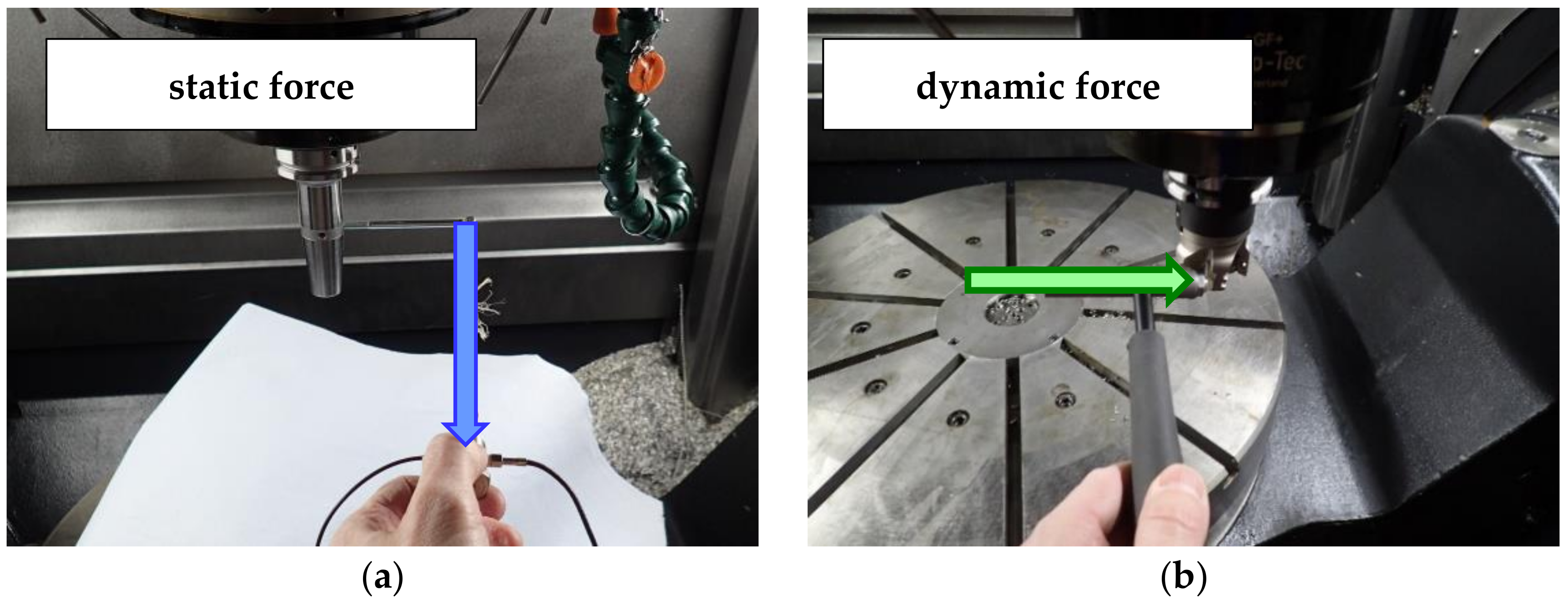
Calibration is defined as the “documented comparison of the measurement device to be calibrated against a traceable reference device”, quoted from [16]. The reference signal is the external force acting in the direction of the calibrated axis, and the calibrated signal is the torque waveform. The first choice is to use the static force as a reference signal; see Figure 1a. This choice has two major drawbacks: (1) when loading the spindle with the static force, the spindle cannot be rotated and, therefore, no correction for idling is possible; and (2), it is complicated to perform the calibration in any machine position because a support structure must be installed to induce larger forces. The second option is to perform the calibration using dynamic force. This can be done using a modal hammer, which has both advantages and disadvantages. The advantages are as follows: (1) the signal from the hammer is dynamic and close to the real cutting forces’, (2) the calibration can be performed while the spindle is rotating, albeit slowly, and (3) the calibration can be performed in any machine position. The main disadvantage when using a modal hammer is that most modal hammers are equipped with an IEPE sensor, which means that the DC component of the signal is filtered out; see [17]. A further complication is the fact that two DAQ systems are needed for the calibration procedure. The first DAQ system collects data from the modal hammer, and the second one is the control system of the machine tool itself, which collects data from the spindle. The two systems generally have different sampling rates, and the measured signals cannot be synchronized. For these reasons, time domain calibration is not possible. The time signal must be converted to the frequency domain and then calibrated there. Advantageously, the number of spectral lines can be chosen when the power spectral density is calculated; see [18]. Then two spectra with the same frequency step are obtained, which can be divided to obtain a “quasi”-frequency response function (FRF or qFRF), see Equation (1).

2.1. Calibration Procedure Description

If we define the dimensionless quantity gain adjust (Ga), according to Equation (2), then, by extrapolating this frequency response function to the null frequency, we can obtain the Ga; see Equation (3). The calibration of the torque measured at the spindle is then performed according to Equation (4).

$$\hat{\mathrm{H}}\left(\mathrm{f}\right)=\frac{{\mathrm{G}}_{\mathrm{calibrated} \mathrm{signal}}\left(\mathrm{f}\right)}{{\mathrm{G}}_{\mathrm{reference} \mathrm{signal}}\left(\mathrm{f}\right)}$$

(1)

$$\mathrm{Ga}=\frac{\mathrm{mean}\left(\mathrm{calibrated} \mathrm{signal}\right)}{\mathrm{mean}\left(\mathrm{reference} \mathrm{signal}\right)}$$

(2)

$$\mathrm{Ga}=\frac{\mathrm{mean}\left(\mathrm{calibrated} \mathrm{signal}\right)}{\mathrm{mean}\left(\mathrm{reference} \mathrm{signal}\right)}=\hat{\mathrm{H}}\left(\mathrm{f}=0\right)$$

(3)

$$\mathrm{mean}\left(\mathrm{corrected} \mathrm{signal}\right)=\frac{\mathrm{mean}\left(\mathrm{measured} \mathrm{signal}\right)}{\mathrm{Ga}}$$

(4)

$$M_k=F_{hammer}·\frac{D_c}{2}$$

(5)

The procedure for calibrating the torque signal from the spindle using the modal hammer force can be summarized as follows:

• The spindle speed is selected. To be able to provide the hit to the tool safely, a practical speed range is between 1 and 10 rpm;
• The torque measurement from the control system is performed twice; first at idle and then with modal hammer taps. When the hammer is tapping, the hammer force signal is also measured;
• The input to the algorithm is three waveforms: the force signal from the modal hammer, the torque signal during idle operation, and the torque signal during operation with modal hammer taps;
• The torque signal from the spindle is corrected for idling (air cut);
• The force signal from the modal hammer is converted to torque using Equation (5);
• The autospectra are calculated from both signals. The periodogram method is used for the calculation. The calculation is unconstrained so that both spectra have the same frequency step (see [18]);
• From the two autospectra, the quasi-frequency response function is calculated according to Equation (1);
• This function is interpolated by a polynomial in order to extrapolate its value at zero frequency. For the regression, we chose the second and higher degree of the polynomial. The main evaluation parameter is the agreement between the frequency response function and the regression;
• The gain factor Ga is calculated according to Equation (3);
• The calibration of the signal measured during machining is performed according to Equation (4).

The calibration procedure is shown graphically in Figure 2.

The apparatus required to perform the calibration is shown in Figure 3. The modal hammer needs to be connected to the DAQ card where the sampling and filtering of the force signal from the modal hammer are performed. Next, the torque on the spindle needs to be measured. This signal is processed analogously to the modal hammer. In this case, the “hammer DAQ system” consisted of an Endevco 2303 modal hammer and an NI cDAQ-9171 + NI 9231 analyzer, which was connected to a DELL Latitude 5510 laptop. The sampling frequency was set to 1600 Hz. The “Control system”, DAQ, was in fact TNCscope software connected to a HEIDENHAIN TNC 640 control system. The sampling frequency was set to 1667 Hz.

The whole calibration procedure is shown graphically in Figure 4. The system force excitation using three groups of multiple hits is presented in Figure 4a. This signal is converted to the time domain signal of the torque by multiplying the excitation signal by the hit point radius; see Figure 4b.

The system response measured on the spindle drive is shown in Figure 4c. As can be seen, there is a basic wavy signal caused by the spindle rotation at a low rpm value. Additionally, there are three groups of peaks visible as a response to the modal hammer excitation. Figure 4d shows the response signal modification: the signal mean value has been deducted from the time domain signal to avoid the signal static component for f = 0 Hz (DC component).

The auto spectrum of both signals (excitation: Figure 4b; response: Figure 4d) is presented in Figure 4e. As can be seen, a useful measurement bandwidth of the spindle is approx. 100 Hz. On the other side, the hammer has a bandwidth of 1 kHz. Thus, the hammer signal is almost constant within the presented region under 100 Hz.

The system transfer gain is calculated as the ratio of the response and the excitation signal using (1), where the reference signal is the excitation signal from the modal hammer recalculated to the torque, and the calibrated signal is the response torque with the eliminated DC component; see Figure 4f. The green curve is the calculated quasi-frequency response function. The calculated gain goes to the infinite high values due to the zero signal of the excitation force at 0 Hz. Thus, the calculated curve was fitted. The polynomial function of the 3rd order was used. The polynomial function is a pure mathematical fit, without any specific physical meaning. The identified function is:

$$\mathrm{y}=p_0·{\mathrm{x}}^0+p_1·{\mathrm{x}}^1+p_2·{\mathrm{x}}^2+p_3·{\mathrm{x}}^3$$

(6)

The gain of the non-calibrated system is 1 because the frequency-dependent gain is usually neglected. These results show that the real system gain is slightly different and should be calibrated for every machine tool before the in-process estimation of the tangential cutting force coefficient.

2.2. Selection of Suitable Modal Hammer and Testing System Linearity

To derive the required excitation torque using the modal hammer, two parameters must be selected: (1) the mass of the modal hammer and (2) the radius of the force moment arm. There are a variety of modal hammers in different sizes available on the market. The hammer must have an acceptable size to fit into the gap between the teeth of the cutter. In this respect, the use of mid-size hammers with a weight range of 100 to 500 g and a diameter of up to one centimeter is an option. The force moment arm is determined by the tool used for machining.

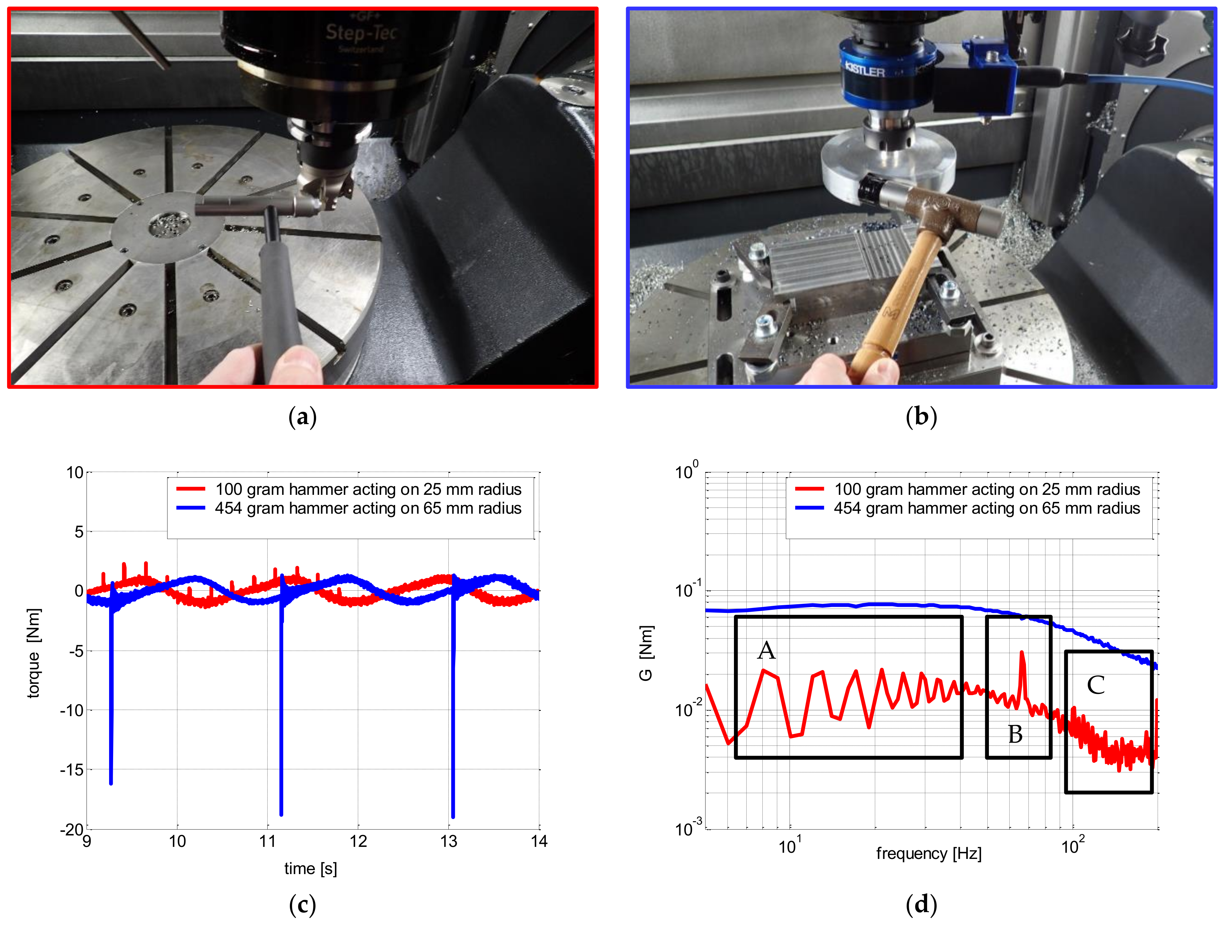
To investigate the effect of the weight and radius on the calibration result, two cases were tested. Case 1 included tapping with a 100 g hammer on a 25 mm radius (see Figure 5a), and case 2 included tapping with a 454 g hammer on a 65 mm radius (see Figure 5b). In this case, we made a special jig because no tool with a sufficient dimension was available. The test was done on a KOVOSVIT MCU700 five-axis machining center with a vertical spindle. Various spindle speeds from 0 to 10 rpm were used for the experiment.

Figure 5c,d show a comparison of the waveform and spectral density of the spindle moment that was excited by the two hammers. The difference in the amplitudes is clearly visible. The ripple in the spectrum marked by rectangle A is due to the rapid repetition of the tapping. The periodic component, B, and the noise, C, are due to insufficient excitation by the smaller hammer. Therefore, to achieve a good signal, it is advisable to choose the largest possible hammer, along with a large instrument diameter. If a sufficiently large tool is not available, a special jig should be made.

The resulting Ga amplification factors are listed in

Table 1. Calibration result for different hammers acting on different radii.

	Case 1	Case 2
	Hammer Mass: 100 g Hit Radius: 25 mm	Hammer Mass: 454 g Hit Radius: 65 mm
Spindle Revolutions:	Obtained Ga [-]:
0 rpm	0.85	0.83
1 rpm	1.03	1.02
2 rpm	1.01	1.00
3 rpm	1.09	1.06
10 rpm	1.14	1.11
$\mu \left(Ga\right)$	1.07	1.05

. The difference in the Ga calibration factors for the zero and non-zero speeds is due to the fact that at zero speed the hammer must also overcome passive resistance in the line. It is, therefore, not advisable to calibrate when the spindle is not rotating. Furthermore, 10 rpm proved to be the maximum speed because, beyond that, it is not possible to tap the tool well.

2.3. Implementation of the Calibration Method on Two Different Machine Tools

The described method was used to the gain identification of two different machine tools with two different spindle types. The first machine was a KOVOSVIT MCU700 five-axis milling center equipped with an electrospindle in the vertical spindle stops. The other machine was a KOVOSVIT MCV2220 three-axis vertical milling center equipped with a belt-driven spindle.

The calibration procedure for both of the machine tools is shown in Figure 6. In both cases, the medium hammer was chosen. A tool with the largest possible diameter was clamped in the spindle. The calibration results are presented in

Table 2. Gain factors and errors corrected by the calibration process.

Machine Tool	Type	Ga [-]	Error [%]
Five-axis machine with electrospindle	MCU700	1.05	5.0
Three-axis machine tool with belt-driven spindle	MCV2220	1.32	32.0

. Since the value of the Ga without calibration is equal to one, the presented results show that a system calibration, before the tangential cutting force coefficient, is required. In the case of the belt-driven spindle, the difference in the gain compared to the non-calibrated condition is 32%. The difference is probably caused by the passive torque of the drive comprehensive kinematic.

3. Validation of the Calibration Method

The system calibration method was validated by tangential cutting force coefficient identification using two different strategies. Firstly, a machine-to-machine comparison was conducted. In this case, the measurements were taken at two different machining centers with the same workpiece machined with the same cutting tool under the same cutting conditions. The calibration factors for both of the machine tools were identified before machining; see Section 2.3. The spindle power was measured using only the control systems of both machines. The tangential cutting force coefficient was calculated for both of the calibrated machines. The validation hypothesis is, if the calibration method is valid, that we will get the same results because the cutting force coefficient is independent of the machine tool type. Secondly, a machine-to-dynamometer comparison was done. Again, the machining was performed with one tool and a workpiece under the same cutting conditions. A KISTLER rotary dynamometer was used in this case. The validation hypothesis is that the results calculated from the calibrated control system data should be the same as the data calculated from the reference dynamometer.

Both components of the tangential cutting force coefficients were calculated using the following procedure: For each test, the torque on the spindle was measured during machining and idling. If the machine was equipped with a dynamometer, the torque of this dynamometer was measured. The torque moments were converted to force. These forces were then corrected according to the procedure described in Chapter 2. The tangential forces arranged as a function of the displacement per tooth were plotted. From these dependencies, the coefficients K_ct and K_et were evaluated using the least squares method using Equations (7) and (8), which define a mean value of the spindle torque, μ (Mk), for down-milling (radial depth of cut a_e) as a function of the mean undeformed chip thickness, μ (h), over one revolution, where D_c is a tool diameter, N_z is the number of teeth, f_z is the feed per tooth, and the tool revolution is parametrized by an angle, φ.

$$\begin{gathered} \mathsf{\mu }\left({\mathrm{M}}_{\mathrm{k}}\right)=\frac{{\mathrm{a}}_{\mathrm{p}}{\mathrm{D}}_{\mathrm{c}}}{2}{\mathrm{N}}_{\mathrm{z}} {{\displaystyle \int }}_{\mathsf{\pi }-\mathrm{acos}\left(1-\frac{2{\mathrm{a}}_{\mathrm{e}}}{{\mathrm{D}}_{\mathrm{c}}}\right)}^{\mathsf{\pi }}({\mathrm{K}}_{\mathrm{et}}+{\mathrm{K}}_{\mathrm{ct}}{\mathrm{f}}_{\mathrm{z}}\sin \left(\mathsf{\phi }\right))\mathrm{d}\mathsf{\phi } \\ \hspace{1em}\hspace{1em}\hspace{1em}\hspace{1em}\hspace{1em}\hspace{1em}\hspace{1em}\hspace{1em}\hspace{1em}\hspace{1em}\hspace{1em}=\frac{{\mathrm{a}}_{\mathrm{p}}{\mathrm{D}}_{\mathrm{c}}}{2}{\mathrm{N}}_{\mathrm{z}} \left({\mathrm{K}}_{\mathrm{et}}\mathrm{acos}\left(1-\frac{2{\mathrm{a}}_{\mathrm{e}}}{{\mathrm{D}}_{\mathrm{c}}}\right)+{\mathrm{K}}_{\mathrm{ct}}·\mathsf{\mu }\left(\mathrm{h}\right)\right) \end{gathered}$$

(7)

$$\mathsf{\mu }\left(\mathrm{h}\right)={{\displaystyle \int }}_{\mathsf{\pi }-\mathrm{acos}\left(1-\frac{2.\mathrm{ae}}{\mathrm{Dc}}\right)}^{\mathsf{\pi }}{\mathrm{f}}_{\mathrm{z}}·\sin \left(\mathsf{\phi }\right)·\mathrm{d}\mathsf{\phi }=\frac{{\mathrm{a}}_{\mathrm{e}}·{\mathrm{f}}_{\mathrm{z}}}{\mathsf{\pi }·{\mathrm{D}}_{\mathrm{c}}}$$

(8)

3.1. Machine-to-Machine Validation

The five-axis and three-axis milling centers mentioned in Section 2.3 were used for the validation experiment. For both machines, a face mill with a diameter of 50 mm for the machining of C45 steel was used. All of the experiment details are provided in

Table 3. Parameters of Case study A.

Parameter	Values
Machined material:	C45 (EN 10083-2-91)
Cutter body:	Walter F4042.B.050.Z05.15|Dc = 50 mm|z = 5
Cutting inserts:	Walter ADMT 160608R-F56|coating WSP45 Insert tip radius: 0.8 mm
Cutting conditions:	vc = 180 m/min ap = 2|3 mm (two levels) ae = 20 mm fz = 0.05|0.10|0.15|0.20|0.25 mm (five levels) down-milling in Y-axis direction
Machine tool 1:	5-axis vertical machining center MCU 700 electrospindle 20 kW|24,000 rpm | transmission 1 HEIDENHAIN iTNC 640 control system
Machine tool 2:	3-axis vertical machining center MCV 2220 Belt-driven spindle 28 kW|8000 rpm|transmission 3.035 HEIDENHAIN TNC 640 control system

. Figure 7 shows the cutter and workpiece used for the machining in this case study.

An example of unprocessed measured signals is shown in Figure 8. The tangential forces calculated using spindle drive power acquired from the control system are shown in Figure 9. As can be seen, the results of both calibrated systems (various machine tools) are very similar. On the other hand, if the systems are not calibrated, the calculated tangential cutting forces differ clearly.

Using the results presented in Figure 9, the resulting tangential cutting coefficients were calculated; see

Table 4. Resulting coefficients, K_ct and K_et. MCU700 data were used as a reference (100%).

ap	Kct [MPa]			Ket [MPa]
[mm]	MCU700	MCV2220	Difference	MCU700	MCV2220	Difference
2	1852 MPa	1846 MPa	0.0%	40 MPa	50 MPa	26%
3	1817 MPa	1850 MPa	2.0%	39 MPa	30 MPa	−23%

. As can be seen, the difference between the values of the cutting component, K_ct, for both levels of the axial depth of cut a_p is very small. Quite a large difference, about 25%, occurred in the case of the edge component. The MCV2220 spindle is driven by an external asynchronous motor with a gearbox. In contrast, the MCU700 is driven by an electric spindle. The huge difference in the MCV2220 values can be attributed to several concurrent factors. The first factor might be the efficiency of the gearbox. For asynchronous motors, it is impossible to find the exact torque constant, and this might be the second factor. The third factor could be the difference between the typical and real motor parameters set in the drive system.

3.2. Machine-to-Dynamometer Validation

The KOVOSVIT MCU700 five-axis milling center mentioned in Section 2.3 was used for the second validation experiment. In this case, an end mill with a diameter of 16 mm for the machining of C45 steel was used. Lower levels of the axial depth of cut were used in this case due to the risk of chatter. All of the experiment details are provided in

Table 5. Parameters of Case study B.

Parameter	Values
Machined material:	C45 (EN 10083-2-91)
Cutter body:	ISCAR HP E90AN-D16-4-C16-07-C Dc = 16 mm|z = 4
Cutting inserts:	ISCAR HP ANKT 070208PNTR Insert tip radius: 0.8 mm
Cutting conditions:	vc = 180 m/min ap = 1|2 mm (two levels) ae = 8 mm fz = 0.05|0.10|0.15|0.20|0.25 mm (five levels) down-milling in Y-axis direction
Machine tool:	5-axis vertical machining center MCU 700 electrospindle 20 kW|24,000 rp|transmission 1 HEIDENHAIN TNC 640 control system
Reference dynamometer:	4-Component Rotating Dynamometer KISTLER 9170A131

. Figure 10 shows the cutter and workpiece used for machining in this case study.

The tangential forces calculated using the spindle drive power acquired from the control system are shown in Figure 11. As can be seen, the results of the calibrated system are very similar to the dynamometer data. In the non-calibrated systems, there are differences in the calculated tangential cutting forces.

Using the results presented in Figure 11, the resulting tangential cutting coefficients were calculated; see

Table 6. Resulting coefficients, K_ct and K_et. The KISTLER dynamometer data were used as a reference.

ap	Kct [MPa]			Ket [MPa]
[mm]	MCU700	KISTLER	Difference	MCU700	KISTLER	Difference
1	2119	2101	−1.0%	67	69	7.0%
2	1838	1804	−2.0%	59	62	11.0%

. The difference between the values of the cutting component K_ct for both levels of the axial depth of cut a_p is very small. A larger, but acceptable, difference of about 10% occurred in the case of the edge component.

4. Results Discussion

The tangential cutting force coefficient is the key parameter characterizing the force interaction between the cutting tool with specific cutting geometry used for the machining of specific workpiece material. The tangential cutting force coefficient can be identified from the machine spindle power signal. The path from the spindle drive to the end of the tool may have a complex design, e.g., in the case of the belt or gear-driven spindles. Thus, it is necessary to calibrate the whole system. This paper presented an operational method based on the excitation of the system using a modal hammer. The main motivation behind this approach was to completely eliminate the need for piezoelectric dynamometers in the calibration procedure. The dynamometers are expensive, and their implementation is time-consuming and often impossible on the shop floor level.

The calibration procedure is described in Section 2.1. The sensitivity to various excitation was also tested. It is necessary to have enough intensive system excitation for a successful calibration. Modal hammers with a higher mass and bigger radius for the hammer hit are recommended, as presented in Section 2.2. Excitation in static (non-rotating) and rotating spindle situations were compared. There is a difference of approx. 15% between the system gain in the static and rotation states. Moreover, the gain increases slightly with higher revolutions (i.e., within the tested range of 1–10 rpm). This shows the influence of the passive torque in the transmission system, which has to be identified and eliminated from the evaluation of the results. The system gain identification must be performed during the spindle rotation. This is in line with the conclusions of Dunwoody [10], Aggarwal [11], and Hänel [19].

The method was first validated using a machine–machine approach. Two machine tools with two different spindles (a motor spindle and a belt-driven spindle) were used for the comparison. The same cutting tool insert type was used for the machining of the same workpiece material on both machines. The identified cutting components of the tangential cutting force coefficient K_ct were almost the same; see Table 2. The difference of the edge component of the tangential cutting force coefficient K_et was about 25%. The bigger difference is related to the low absolute values of the coefficient and also to the fact that the edge component is related to the static component of the cutting force, which cannot be identified perfectly using the modal hammer. The machine–machine validation also shows that the method is universal and can be used on the shop floor level for the calibration of different machine tools to obtain comparable cutting process monitoring results.

Subsequently, a machine-dynamometer validation was also conducted. Again, the results of the cutting component based on the spindle data and results based on the reference dynamometer measurement data were very similar (a difference of about 2%). The error of the edge component was about 10%, see Table 6. In general, both components of the identified tangential cutting force coefficients were dependent on the axial depth of cut ap in all of the tested cases. The reason was the relatively low ap used compared to the insert tip radius.

Furthermore, we can compare our results with the traceable results of other researchers. De Menezes Silva states in [20] that for AISI 1095 carbon steel, the K_ct parameter is equal to 2500 MPa. By comparing the tensile strengths of AISI 1095 and EN C45 steel, a recalculation of the tangential component of the specific cutting force comes out to be around 1700 MPa. This correlates well with the results in Table 4 and Table 6.

As a further research direction, the calibration of all other controlled machine axes can be identified.

5. Conclusions

A procedure for calibrating the spindle torque signal for the tangential cutting force coefficient estimation was proposed. The calibration procedure was based on the tap test using the modal hammer excitation and the spindle power signal response. The proposed procedure was successfully validated using a machine–machine comparison approach and a machine–dynamometer comparison approach. The novelty of the proposed method is in the use of the modal hammer as the main measuring device instead of the typically used dynamometers. Thus, the method is applicable on the shop floor level even if large workpieces are already clamped on the machine table.