Abstract
Inspired by rodents’ free navigation through a specific space, RatSLAM mimics the function of the rat hippocampus to establish an environmental model within which the agent localizes itself. However, RatSLAM suffers from the deficiencies of erroneous loop-closure detection, low reliability on the experience map, and weak adaptability to environmental changes, such as lighting variation. To enhance environmental adaptability, this paper proposes an improved algorithm based on the HSI (hue, saturation, intensity) color space, which is superior in handling the characteristics of image brightness and saturation from the perspective of a biological visual model. The proposed algorithm first converts the raw image data from the RGB (red, green, blue) space into the HSI color space using a geometry derivation method. Then, a homomorphic filter is adopted to act on the I (intensity) channel and weaken the influence of the light intensity. Finally, guided filtering is used to process the S (saturation) channel and improve the significance of image details. The experimental results reveal that the improved RatSLAM model is superior to the original method in terms of the accuracy of visual template matching and robustness.
1. Introduction
The SLAM system proposed by Milford et al. from the University of Queensland in 2008, known as RatSLAM [1], is a computational model based on the hippocampus of rodents. With the discovery of “pose cells”, “head orientation cells”, and “grid cells” in the hippocampus of rodents [2,3,4], the RatSLAM system has gradually gained research attention. In the RatSLAM system, odometer information was provided by a camera sensor based on pure vision [5,6]. RatSLAM not only has biological rationality but is also suitable for indoor and outdoor positioning and mapping. Moreover, it has the advantages of low algorithm complexity and high speed in outdoor navigation [7]. Although the RatSLAM algorithm relying on pure vision has been used well, it exposes deficiencies, such as low reliability, limited image matching accuracy, and poor environmental adaptability under environments with changes in light [8]. With the change in light intensity, the gray image of the same scene has different values because of the different brightness. In the same scene, different gray values lead to errors in visual template matching, which affects loop-closure detection and the accuracy of the experience map [9]. To solve the problem of map deterioration caused by light change, we attempt to seek a reasonable method for enhancing the robustness of the system by restraining the illumination change.
Many researchers have improved different aspects of the RatSLAM algorithm, yet the improved methods are not very flexible in scenes with lighting changes. To solve the loop-closure problem, Sun, C et al. used a fast and accurate descriptor called ORB (oriented fast and rotated brief) as the feature matching method [10]. Accordingly, Kazmi et al. used the Gist descriptor as the feature matching method, which can also reduce the matching error in traditional RatSLAM [11]. Using a descriptor of features can help increase the precision of loop-closure detection by improving the accuracy of feature matching. To compensate for the odometer error, Tubman et al. added a grid map into the system to describe environmental features with a 3D structure [12], which is very similar to the RGB-D-based RatSLAM system proposed by Tian et al. [13]. The results showed that both methods could solve the problem of missed feature points caused by white walls. Salman et al. integrated a whisker sensor that can move along three axes into the system to form a Whisker-RatSLAM [14]. Their preprocessed tactile method and control scheme can reduce the error of a robot’s pose estimation to a certain extent. Milford et al. used multiple cameras instead of a single monocular camera in the visual odometer [15]. The combination of data from multiple cameras provided more-accurate 3D motion information, thus substantially promoting map quality. From the aspect of bionics, Silveira et al. extended the original RatSLAM system from a 2D ground vehicle model to an underwater environment with a 3D model. The system they created is a dolphin SLAM based on mammalian navigation [16]. Using a mouse-sized robotic platform as an experimental vehicle, Ball et al. changed the significance of visual cues and the effectiveness of different visual filtering techniques [17,18]. In their improvement, the vision sensor’s field of vision was narrower and closer to the ground, which avoided the effect of visual angle on the formation and use of cognitive maps.
Why does light change have a substantial effect on the RatSLAM system? The reason is that the traditional RatSLAM system is based on the SAD (sum of absolute differences) matching model for visual template matching [19]. This matching method calculates the image gray value, which will be affected by the change in illumination. In response to the effect of light, Glover et al. associated the local feature model in FAB-MAP with pose cell filtering and an experience map in RatSLAM [9]. They created a hybrid system that combines RatSLAM with FAB-MAP. The illumination invariance data provided by FAB-MAP are the key of the RatSLAM system to addressing the challenge of illumination change. Therefore, they obtained an accurate experience map through data association. In contrast to Glover’s method, it is a feasible method for processing the illumination in the image processing part of the algorithm. There are many studies in the field of image processing on suppressing illumination changes, and using a homomorphic filter is a typical and effective method for achieving results [20]. In addition, the HSI color space is a flexible and convenient way to treat image brightness separately in image processing [21]. If the HSI color space and homomorphic filter can be combined, it will produce better results.
In order to improve the mapping accuracy of RatSLAM and solve the problems caused by the changing light in environments, this paper proposed to apply the HSI color space on RatSLAM system from the perspective of bionics. In the front-end part of visual processing, the HSI color space with biological visual characteristics was added to further enhance the integrity of the bionic system, which lays a foundation for exploring a more intelligent robot navigation system. The combination of RatSLAM with a biomimetic mechanism can not only raise the robustness of the system but also compensate for the lack of a biological vision mechanism in the visual part of the RatSLAM system. Experimental results on various scenes and open datasets showed that the proposed method achieved better visual template accuracy, mapping accuracy, and system robustness than traditional RatSLAM.
The remainder of this paper is arranged as follows. Section 2 describes the traditional RatSLAM algorithm and the problem of adaptability it faces. Section 3 proposes the improved RatSLAM algorithm, integrating the HSI color space. Section 4 verifies the improvement in the robustness of the proposed method through four scenes of drawing experiments. Finally, Section 5 concludes the contribution of this paper and the shortcomings to be overcome in future work.
2. RatSLAM Model
By imitating the computational model of navigation in the hippocampus of a rodent brain, RatSLAM provides a SLAM solution that consists of three components: pose cells, local view cells, and the experience map [22]. Pose cells are established in competitive attractor network models (CANs), and the information of a robot’s posture in a two-dimensional plane is represented by the position and direction of pose cells. Local view cells are used to record the visual information obtained by a robot, encode the recorded information, and correct the accumulated errors. The experience map is a topological map used to store environmental information, in which the navigation error can be corrected by loop-closure detection.
2.1. Pose Cells
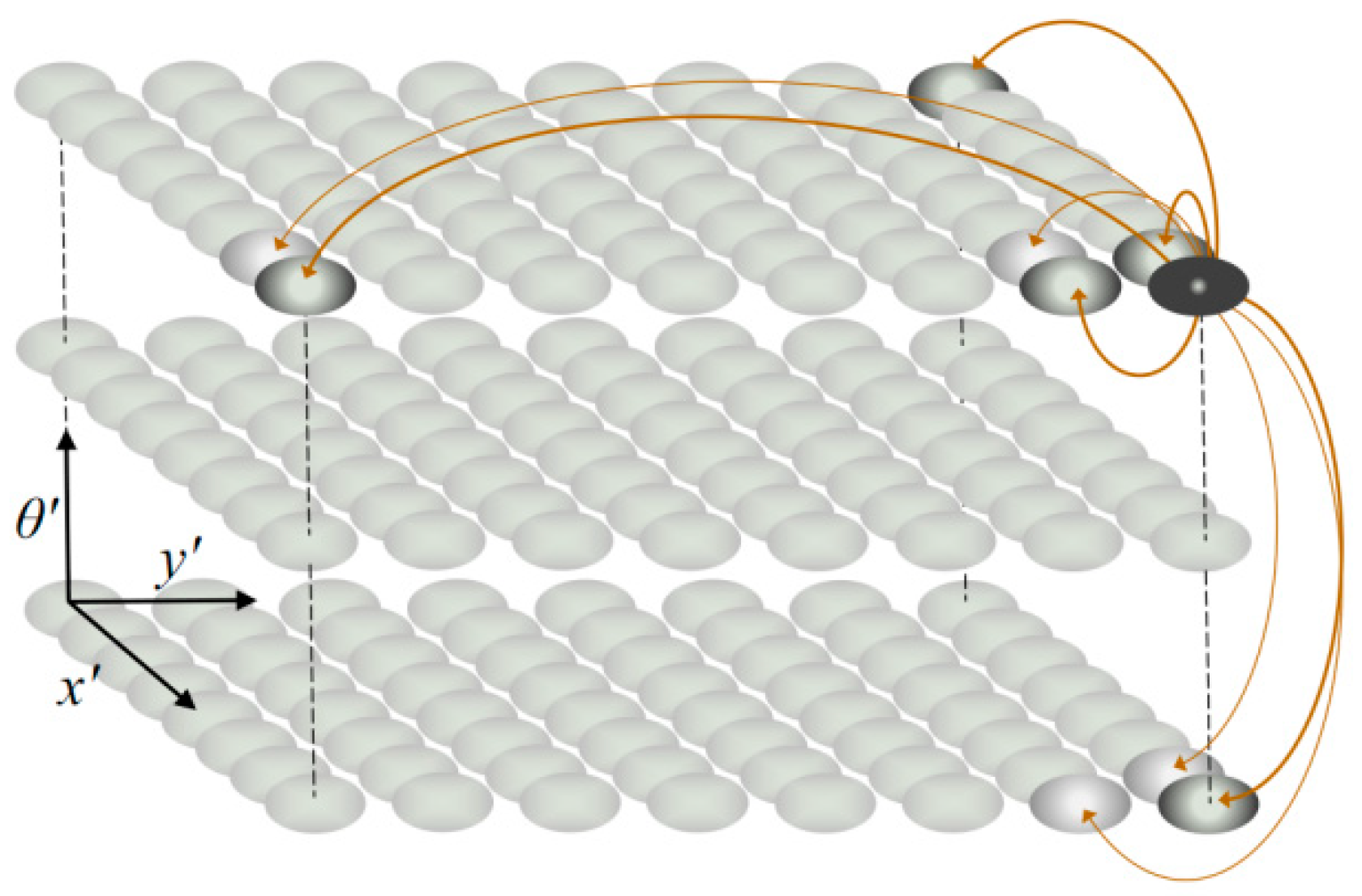
Pose cells constitute the core of RatSLAM system dynamics, which is described by a three-dimensional CAN model. In this three-dimensional structure, the active point affects its surrounding points, and the boundary points are connected to the opposite side to form a wrapped structure, as shown in Figure 1. When moving in large environments, the active pose cell generates an energy emission field to form a self-positioning mode that is similar to the grid cell [6]. A pose cell is denoted as P(x′,y′,θ′) in the three-dimensional coordinate system, where (x′,y′), θ′, and P represents the position, head direction, and degree of the cell’s activation, respectively.
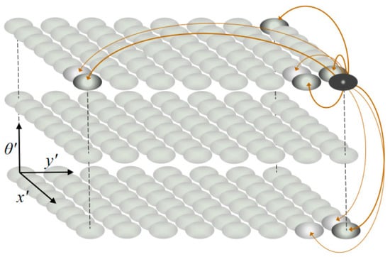
Figure 1.
Three-dimensional competitive attractor network (CAN) model.
2.2. Local View Cell
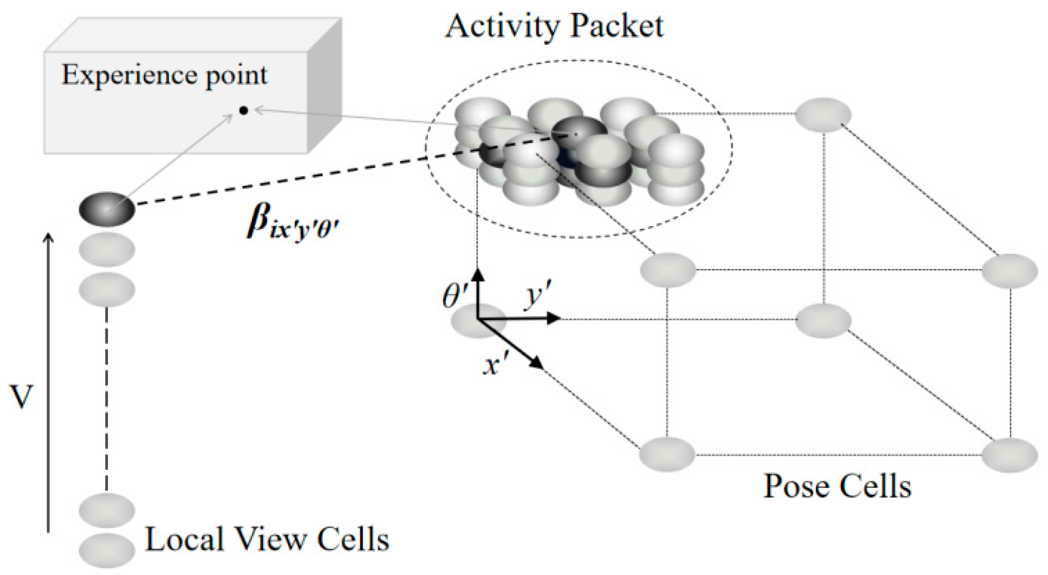
Local view cells are primarily used to store visual templates, which are indispensable for map construction and positioning systems [23]. There are two types of interactions between local view cells and pose cells simultaneously: map construction by associative learning from each other and localization update by injecting activities into pose cells [24]. As shown in Figure 2, local view cells encode scene information in video sequences, and connections exist between pose cells and local view cells through β (weighted connection between them). Visual templates are matched by using the SAD model. Once the matching is successful, the pose cells are updated as a historical scene that has been revisited. Although the SAD matching method is simple and fast, it is greatly affected by illumination, which will result in low robustness of the system.
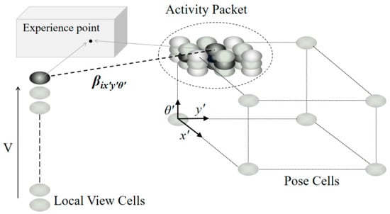
Figure 2.
Local view cells and pose cells.
2.3. Experience Map
The experience map exported by the RatSLAM system is a topological graph composed of a set of individual experience points demonstrated by {ei}i=1,…,n. Each experience point ei contains pose cell information Pi, the serial number of the visual template Vi, and location information pi. An experience point can be expressed as ei = {Pi, Vi, pi} [25].
2.4. Effect of Light and Solution
RatSLAM corrects the accumulated error of the visual odometer by applying optimization introduced from detected loop closures in the experience map. The SAD model is adopted to compare the similarity of two scenes to determine whether loop closure occurs. One of the key factors affecting loop closure is the variation in illumination intensity, which is a phenomenon that often occurs indoors and outdoors. For example, experiments in outdoor environments on a large scale always have changing sunshine. This situation causes the RatSLAM system to be unable to recognize the loop closure that should be recognized, thereby resulting in a severe mapping error. Moving objects blocking the light in indoor environments also have this effect on the RatSLAM algorithm.
In contrast, human beings easily distinguish the same scene with different illumination. This is because cone cells and rod cells in the human visual system can sense light intensity so that people can make a correct judgment of the same scene with different brightness [26]. Following the mechanism of human visual system modeling, this paper added a biological vision model called the HSI color space into the original RatSLAM system to improve its performance in environments with variant illumination.
3. RatSLAM with HSI Color Space
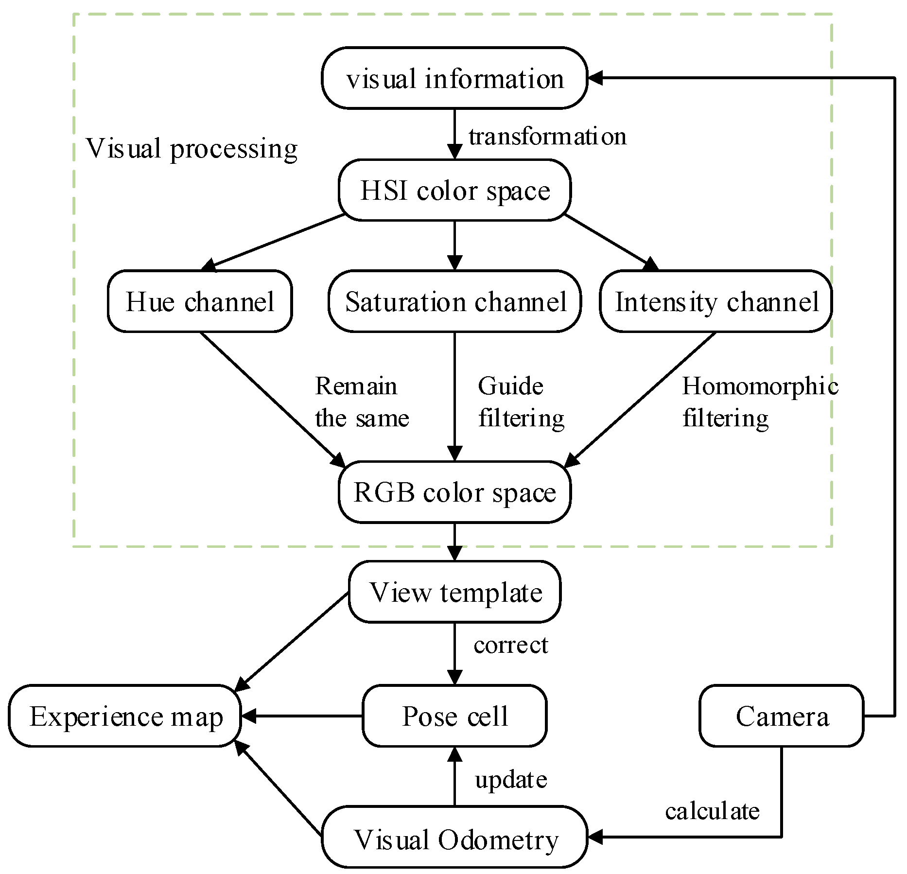
In this paper, three independent channels were formed after the RGB color space was converted to the HSI color space. The intensity channel was first processed with homomorphic filtering to weaken the low-frequency signal and enhance the high-frequency signal to suppress the light and enhance the details. Then, the saturation channel was treated using guided filtering to enhance the saturation change information to advance the effect of detailed information. The hue channel remained the same. After the intensity single channel and saturation channel were processed, the HSI color space was converted to the RGB color space again. The improved system retained the SAD matching method used by the RatSLAM system. Homomorphic filtering reduces the influence of illumination components, and the introduction of guided filtering enhances the image details. The above steps lay the foundation for improving the robustness of the system. Figure 3 shows the framework of the proposed method.
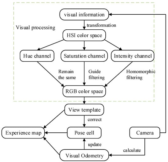
Figure 3.
Framework of bionic navigation algorithm based on HSI color space.
3.1. HSI Color Space
When looking at a colored object, we describe it by its hue, saturation, and intensity. These characteristics describe the color attribute of the pure color, the brightness of the color, and the subjective descriptor by humans [27]. The HSI color space describes color through hue, saturation, and intensity by a mathematical model of bionic vision based on the human visual system. The three components in this space are independent of each other, so it is of great benefit to develop image processing algorithms according to their decoupling [28].
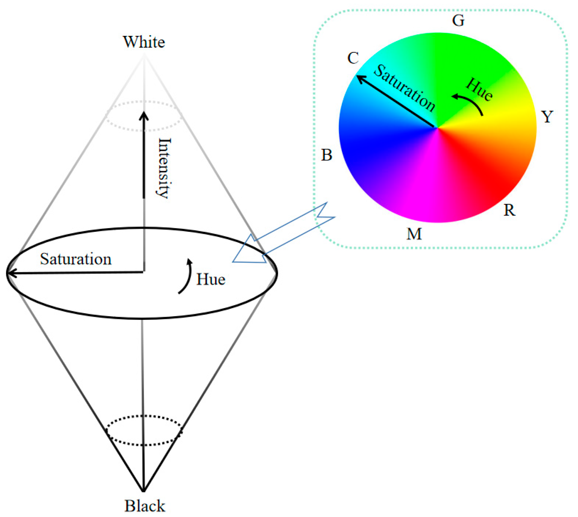
Figure 4 demonstrates that the HSI color space can be described by a combination of two cones. The central plane of the two cones is a circle of radius 1. The circular angle ranges from 0 to 2π, which is used to represent the hue component in the HSI color space. The distance from one point to the center of the circle represents saturation, and its range is 0–1. The upper and lower axes represent light intensity components, with values ranging from 0 (black) to 1 (white). Compared with RGB space, HSI space not only is closer to human perception of color but can also resist the inference of noise [29,30].

Figure 4.
Biconical HSI color space model.
3.2. Transformation between HSI Space and RGB Space
In this paper, geometric transformation was used to transform RGB space into the HSI color space. Images transformed into the HSI color space by this method have higher distinguishing ability, and therefore, it is more suitable for the RatSLAM system. The value of the hue component H is in the range of [0, 2π], representing colors from red to purple, as shown in Equations (1) and (2) [31,32].
The saturation S, given by Equation (3), ranges from 0 to 1.
The intensity I is the arithmetic average value of RGB values.
3.3. Homomorphic Filtering
The performance of RatSLAM deteriorates in environments with varying illumination. To correct this flaw, our work addressed illumination in the frequency domain of images. According to Equation (5), an image f(x, y) can be considered as the product of its illumination component i(x, y) and its reflection component r(x, y) [33].
The illumination component i(x, y) belongs to the low-frequency component, changes slowly, and reflects the illumination characteristic, while the reflection component r(x, y) belongs to the high-frequency component and reflects the details of an image [34]. To address problems arising from images with insufficient or uneven illumination, the image’s low-frequency component must be reduced while enhancing the high-frequency component as much as possible. A homomorphic filter can help reduce the image illumination component to suppress the influence of illumination in the RatSLAM system. Logarithm transformation of Equation (5) yields
By applying a Fourier transformation to Equation (6), a frequency domain expression can be achieved as in Equation (7). The frequency domain approach helps to adjust the brightness by separating high-frequency components from low-frequency components.
To weaken the low-frequency component and enhance the high-frequency component, the homomorphic filter should be a high-pass filter. A Gaussian high-pass filter was defined as in Equation (8):
In order to easily control the frequency gain range, Equation (8) was modified slightly to get Equation (9) as the filter.
where D0 is the cutoff frequency, which will affect the result of the filter. Rh is the high-frequency gain and Rl is the low-frequency gain. The filter should satisfy Rh > 1 and Rl < 1, which will reduce the low-frequency component and increase the high-frequency component. The sharpening coefficient c was used to control the sharpening of the bevel of the filter function, and its value also affects the output. D(u,v) is the distance from the frequency rate (u,v) to the center of the filter. The homomorphic filter was multiplied with the frequency domain expression and the frequency domain signal was filtered as followed:
An inverse Fourier transformation was applied to Equation (10) to obtain the spatial expression as follows:
The component of channel I after homomorphic filtering is the exponent of Equation (11):
3.4. Guided Filter
Fitting to the HSI color space, the guided filter was selected as to process the saturation channel to enhance the image quality and ensure the accuracy of the image matching. An image can be expressed as a two-dimensional function, which has a linear relationship between image input and output in the two-dimensional window.
where qi represents the output images and I is equal to S in Equation (3), i is the index of the image I and ωk is the range of values of i. ak and bk represent the coefficients of the linear relationship [35].
The gradient of Equation (13) is Equation (14). Equation (14) reveals that the input and output have similar gradients, which is why the guided filter maintains the edge characteristics.
The next step is to find the appropriate coefficient to minimize the difference between the output value and real value. This process can be described by
where pi is the grayness value of pixel i in the input matrix, and εak is the penalty term. The values of ak and bk can be calculated by the least squares method as Equations (16) and (17) [36].
where ω is the number of pixels and μk and σk are the mean and variance of the input I, respectively. is the mean of p and ε is equal to 0.8 here.
Using the saturation channel as the input and output of the guided filter can enhance the edge effect of the image. The edge of the saturation channel represents the gradient of the gray value. Enhancing the edge of the saturation channel is equivalent to enhancing the saturation change information, which makes the image more obvious at the color boundary [37]. Compared with a blurred image, an image with an obvious color difference is more suitable for template matching.
3.5. The Effect of Biological Vision Modeling
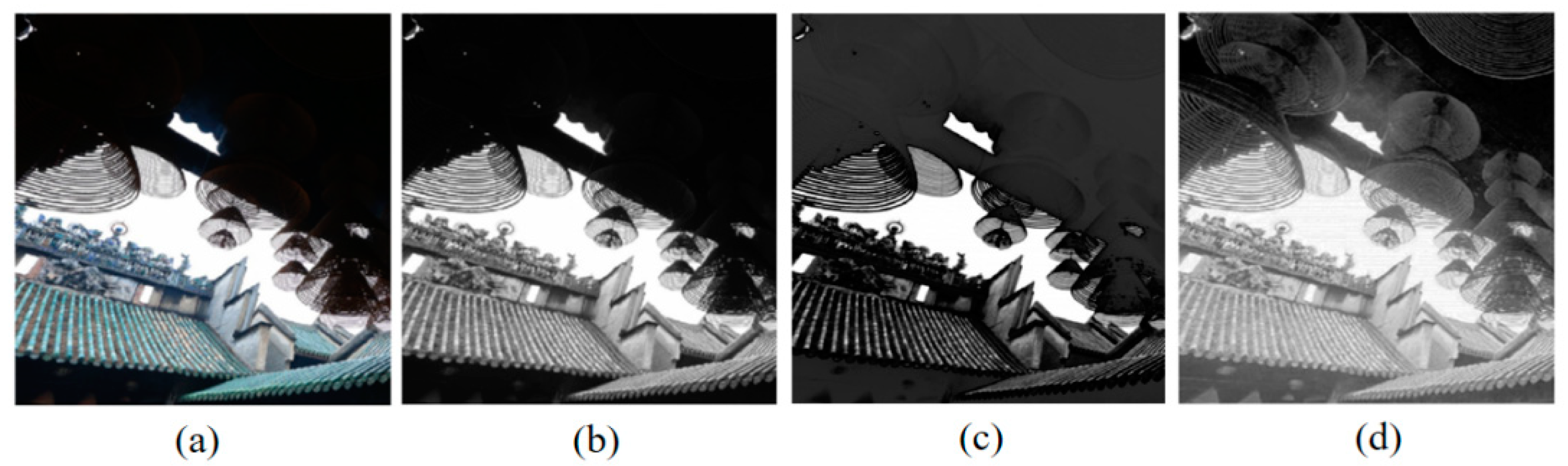
An example was used to illustrate the results of the S channel and I channel in the HSI color space that were converted from RGB color space. Figure 5a is the original image, Figure 5b is the gray image of the original image, Figure 5c is the image processed based on the frequency-tuned (FT) model [38], and Figure 5d is the gray image after its S channel and I channel were filtered. The details of the dark part of the original image are improved, and the entire image is clearer than before. Because the homomorphic filter enhances the high-frequency part of the image and weakens the low-frequency part of the image, the overall brightness of the image is improved. When the input image of the guided filter is the same as the processed image, it has the function of enhancing the edge characteristics of the image, which increases the image quality and is more conducive to template matching, as shown in Figure 5d. Compared with Figure 5b, the feature significance in Figure 5c is improved, which is another method to improve visual template matching from the image processing part [38]. However, there is less image information in the dark part of Figure 5c, which will affect the system output in the case of an image with uneven illumination.

Figure 5.
Results of biological vision model and FT model. (a) Original RGB image; (b) grayscale image of the original image; (c) grayscale image processed by FT model; (d) the grayscale image processed by biological vision model.
4. Experiments
An experimental platform was built to verify the feasibility and effectiveness of the method proposed in this paper. The experiments included filter parameter adjustment, module ablation, image matching, and analysis of the visual template and the effect of mapping in four scenes.
4.1. Experimental Setup
4.1.1. Experimental Equipment
Three sets of data from indoor and outdoor experiments were collected to assess the feasibility and accuracy of the proposed algorithm. An Osmo Pocket camera (Xinjiang Innovation Company, Shenzhen, China) with a field of view (FOV) of 80°, a sampling frequency of 25 Hz, and a resolution of 1080 p was used to collect video data.
4.1.2. Evaluation Criteria
Precision and recall were chosen as the criteria for evaluating the performance of loop-closure detection before and after the proposed method of using a biological vision model. However, an increase in precision may lead to a decrease in recall, and vice versa. Therefore, F values or precision–recall curves are often used to evaluate the results of loop-closure detection.
The precision is the ratio of true positives (TPs) to the sum of TPs and false positives (FPs). It can be expressed as
The recall rate is the ratio of TPs to the sum of TPs and false negative numbers (FNs), which can be written as
The F value is defined as
4.2. Parameter Selection of Filters
Parameters that affect the results of the homomorphic filter include the high-frequency subsection Rh, the low-frequency subsection Rl, the sharpening coefficient c, and the cutoff frequency D0. Rh should be greater than 1, while Rl should be less than 1. The value of c should be between Rl and Rh, while the value of D0 should fluctuate around 10 according to experience [39]. A homomorphic filter improves the overall pixel brightness, but it is not as always true that the greater the brightness, the higher the image quality. Image information entropy, pixel mean value, and pixel variance were used as criteria to evaluate the filtering results, and a part of the parameter setting is shown in Table 1.

Table 1.
Experimental results of filtering parameters.
As shown in the lower part of Table 1, when ε rises to about 0.8, the information entropy of the image will not rise. Therefore, in the guided filtering, ε = 0.8 can achieve good results [40].
4.3. Ablation Studies of Two Modules
Modules of the homomorphic filter and the guided filter were added in the image processing section, and the effects of these two modules on the system were verified by ablation experiments. Figure 5 was taken as the input image, the homomorphic filter and guided filter were separately added into the system, and the information entropy and other elements of the image were calculated. The experimental results are shown in Table 2. Experimental results show that the two fusion modules can achieve better results.
Table 2.
Ablation study results of two filter modules.
4.4. Analysis of Image Similarity and SAD Results
In the RatSLAM system, the SAD model is used for view template matching. Two images are considered as different scenes only if the difference between their SAD models is greater than a threshold value. Otherwise, loop closure is detected. Cosine similarity is a method for evaluating the similarity of two images. It is suitable for assisting in the judging of template matching results and can be presented as in Equation (21), where Xi and Yi are two different vectors. The closer the cosine result is to 1, the more similar the two images are.
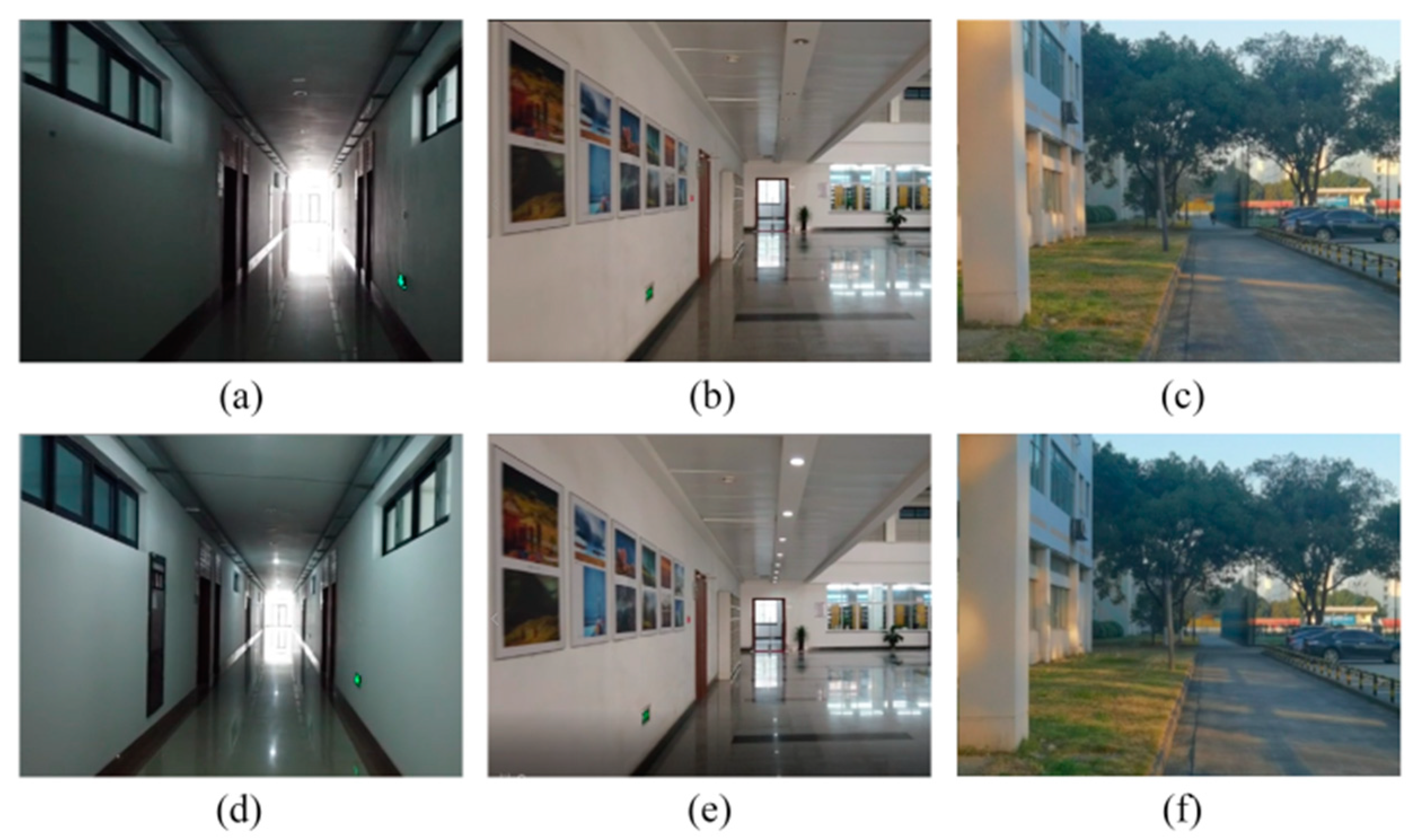
Three sets of images corresponding to loop closure in different experimental scenes were chosen to compare the proposed method and traditional RatSLAM in regard to view template matching. As shown in Figure 6a–c there were three scenarios, and their corresponding loop-closure scenarios are shown in Figure 6d–f, respectively. The scenarios in Figure 6d–f have changes in light intensity compared to their first scene.
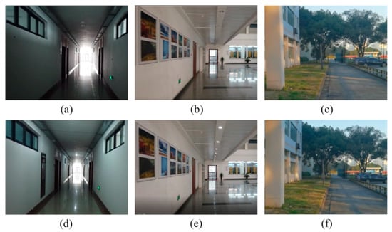
Figure 6.
Three experimental scenarios. In (a) the corridor light is off; in (b) the library light is off; (c) is the first campus path; in (d) the corridor light is on; in (e) the library light is on; (f) is the second campus path.
Through two sets of experiments before and after using biological vision modeling, the SAD template matching result and cosine value were calculated, as shown in Table 3. The SAD values of the HSI-based system were 0.325, 0.033, and 0.023, which were smaller than those of traditional RatSLAM. These results mean that the two visual templates matched better. The cosine values of the HSI-based system were 0.901, 0.996, and 0.998. The two images after improvement were more similar, and the system was able to easily judge whether they are loop closures because the results were closer to 1 than those of the original system.
Table 3.
Comparison of SAD results and cosine similarity before and after system improvement.
4.5. Analysis of Visual Template and Experience Map
Analysis of the results focused on the aspects of visual templates and experience maps. By collecting the experimental data of four scenes, the RatSLAM method based on the HSI color space was compared with the traditional RatSLAM in terms of the results of loop-closure detection and accuracy of experience map. Because the first two scenes had changing lighting, comparisons with the FT-model-improved method were made to validate the effectiveness of the proposed biological vision model–based method proposed.
4.5.1. First Scene: Mechanical Building Corridor
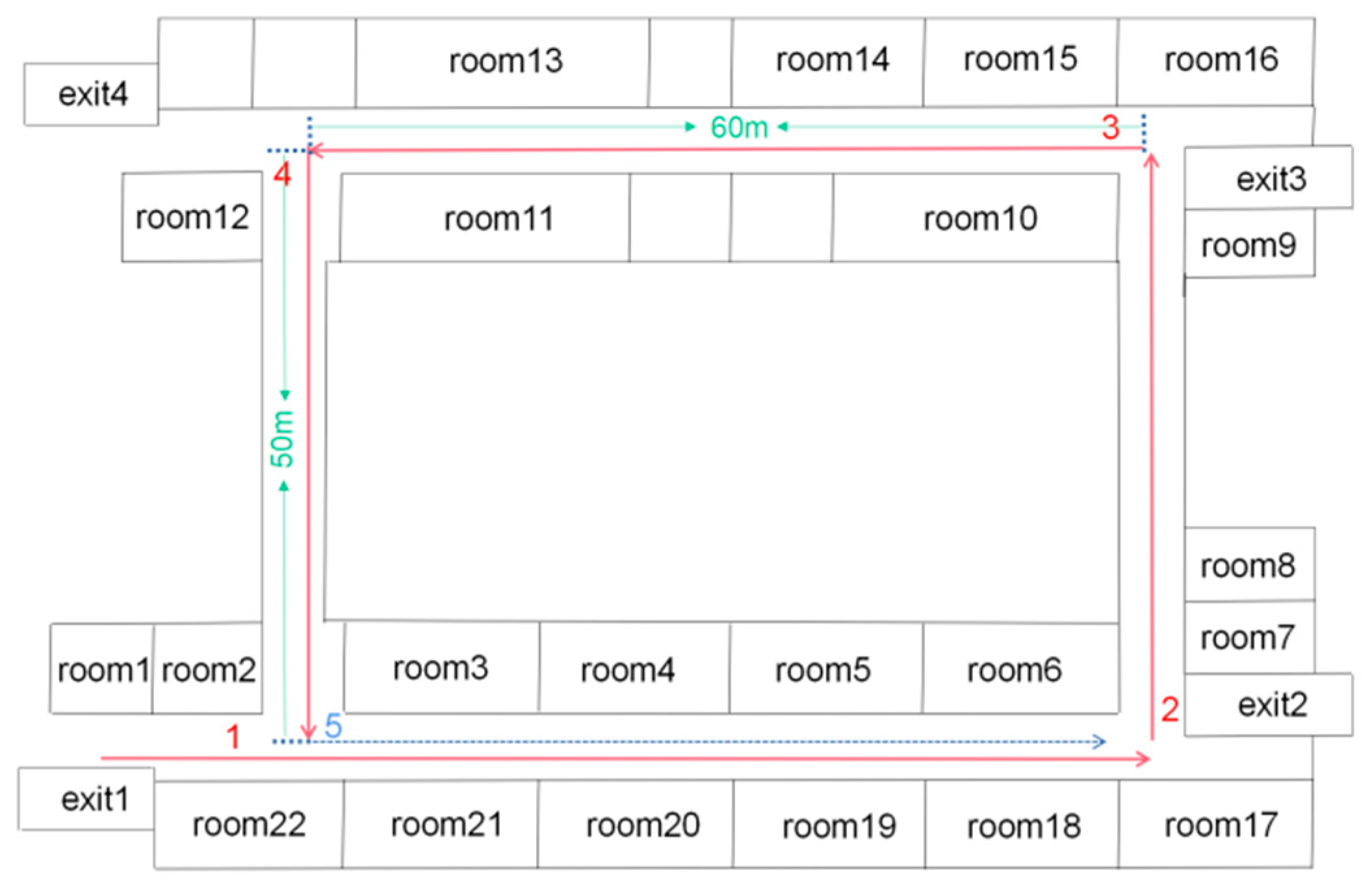
The first experiment was performed in the Mechanical Building of Soochow University, Suzhou, China. Figure 7 shows the path in its corridor. The red solid lines and the blue dashed line represent the first and second paths, respectively. To validate the robustness and adaptability of the proposed algorithm to illumination variation, the lights in the corridor were turned out when we reached the loop-closure point (trajectory labeled 5 in Figure 7). The blue dashed line indicates the closed-loop path when the lights were off.
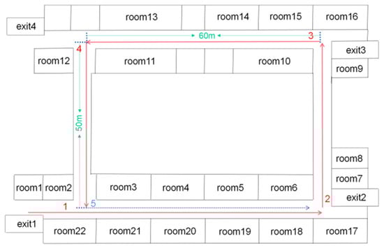
Figure 7.
Schematic of the mechanical building.
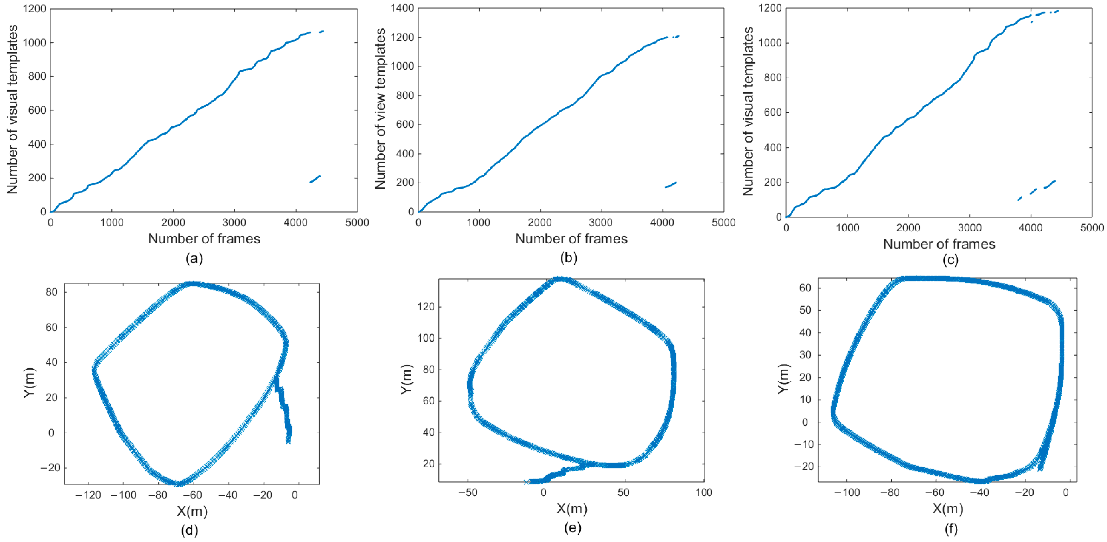
In Figure 8a–c, the horizontal coordinates represent the number of frames, and the vertical coordinates represent the number of visual templates. Overall, the number of visual templates increased with the number of frames. Figure 8a is a visual template derived from the original RatSLAM algorithm in the first scene. Figure 8b was generated by the FT model, Figure 8c corresponds to Figure 8a,b, and it was derived from the RatSLAM algorithm incorporating biological visual modeling in the same scene. Comparing Figure 8a,b with Figure 8c shows that the visual template identified more loop-closure locations after it was improved by the biological visual model. In fact, there should be a loop closure after 3600 frames. However, the original RatSLAM algorithm only recognized the loop closure at approximately 4300 frames and the RatSLAM method based on FT model recognized the loop closure at approximately 4000 frames. Adopting biological visual modeling can bring forward the first loop-closure detection to the 3700th frame, together with increasing the number of TPs, as shown in Figure 8c. The method of the HSI model improves the overall brightness of the image and solves the problem of uneven illumination. Therefore, in the scene with changing illumination, this method can recognize more loop-closure visual templates than the traditional RatSLAM and the method of FT model.
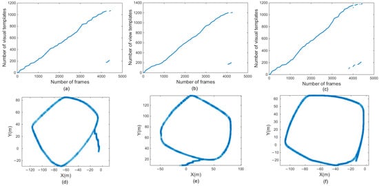
Figure 8.
Experimental results of the first scene. (a,d) are visual templates and experience map output by traditional RatSLAM. (b,e) are visual templates and experience map output by RatSLAM based on FT model. (c,f) are visual templates and experience map output by RatSLAM based on HSI model.
Figure 8d–f are the experience maps of first experiment corresponding to the original RatSLAM, FT model improved method, and the proposed method, respectively. The improved RatSLAM based on the HSI color space had better robustness and could identify the loop closure where it should be recognized, while the original algorithm and the method of FT model only recognized the loop closure in the second half of the loop closure, which greatly affected the accuracy of the final experience map. The FT model improved the significance of features in the image, ignored nonsignificant features, and achieved the effect of increasing matching accuracy. However, in the scene of varying illumination, the FT model could not recognize the loop closures of the system. The traditional RatSLAM will face different illumination intensity when passing through the same place twice in the scene. At this time, it cannot accurately identify the loop closure, while the improved method based on HSI model can solve this problem.
4.5.2. Second Scene: Second Floor of the Library Lobby
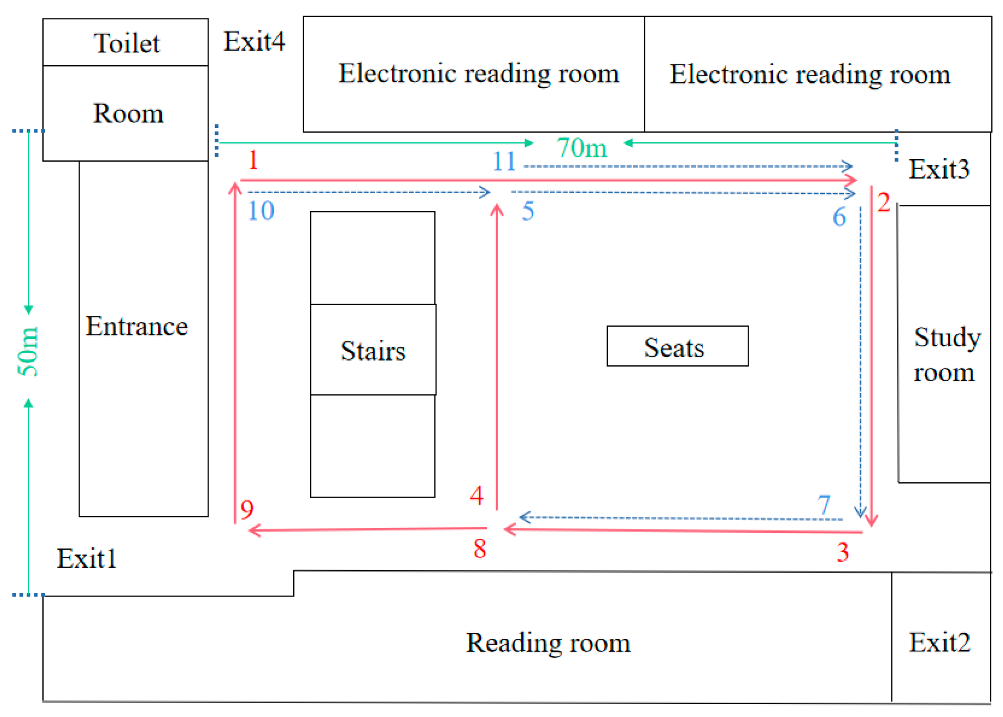
The 8-shaped path data of the second-floor lobby of the Soochow University Library were collected to verify the robustness and adaptability of the improved algorithm. The second scene was slightly more complex than the first scene. The red solid lines and blue dashed lines in Figure 9 together represent the path, in which multiple loops exist. The path indicated by the blue dotted line was repeated, and the loop closure was the path of 5->6->7 and the path of 10->11.
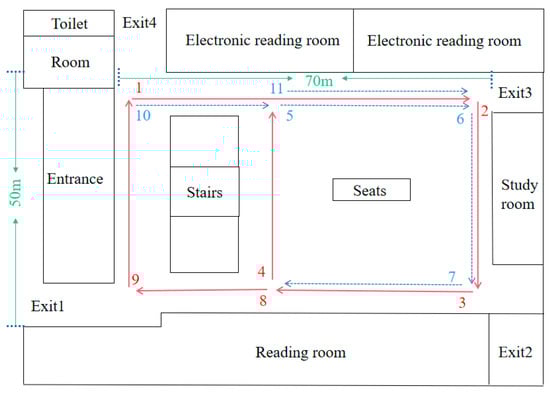
Figure 9.
Hall on the second floor of the library.
Figure 10a–c are the changes in number of frames and visual templates obtained by traditional RatSLAM algorithm, RatSLAM algorithm based on FT model, and RatSLAM algorithm improved by the HSI model in the library scene, respectively. Affected by light changes, between 1000 and 1500 frames, the number of detected loop closures by the original RatSLAM algorithm and FT model-improved algorithm was fewer than that of the biological visual method. In terms of the number of loop-closure points after 2000 frames, the improved algorithm had more loop-closure points, which is shown as the length of the lines composed of loop-closure points in Figure 10c.
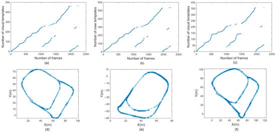
Figure 10.
Experimental results of the second scene. (a,d) are visual templates and experience map output by traditional RatSLAM. (b,e) are visual templates and experience map output by RatSLAM based on FT model. (c,f) are visual templates and experience map output by RatSLAM based on HSI model.
Figure 10d–f are the experience maps of library scenes obtained by the above three methods. Loop closures can be recognized by original RatSLAM, the method based on the FT model, and the proposed improvement based on HSI model. The analysis of visual templates shows that the RatSLAM algorithm based on the biological vision model had more loop closures. Because more historical visual templates are identified, the improved method based on HSI model will have more TPs, which has an important impact on the accuracy of mapping. Compared to the original RatSLAM algorithm, the number of FPs produced by the algorithm based on the HSI model was reduced. The end of Figure 10d shows that the path deviation was larger, while Figure 10f had a relatively smaller deviation at the end.
4.5.3. Third Scene: Jingwen Library and Wenhui Building
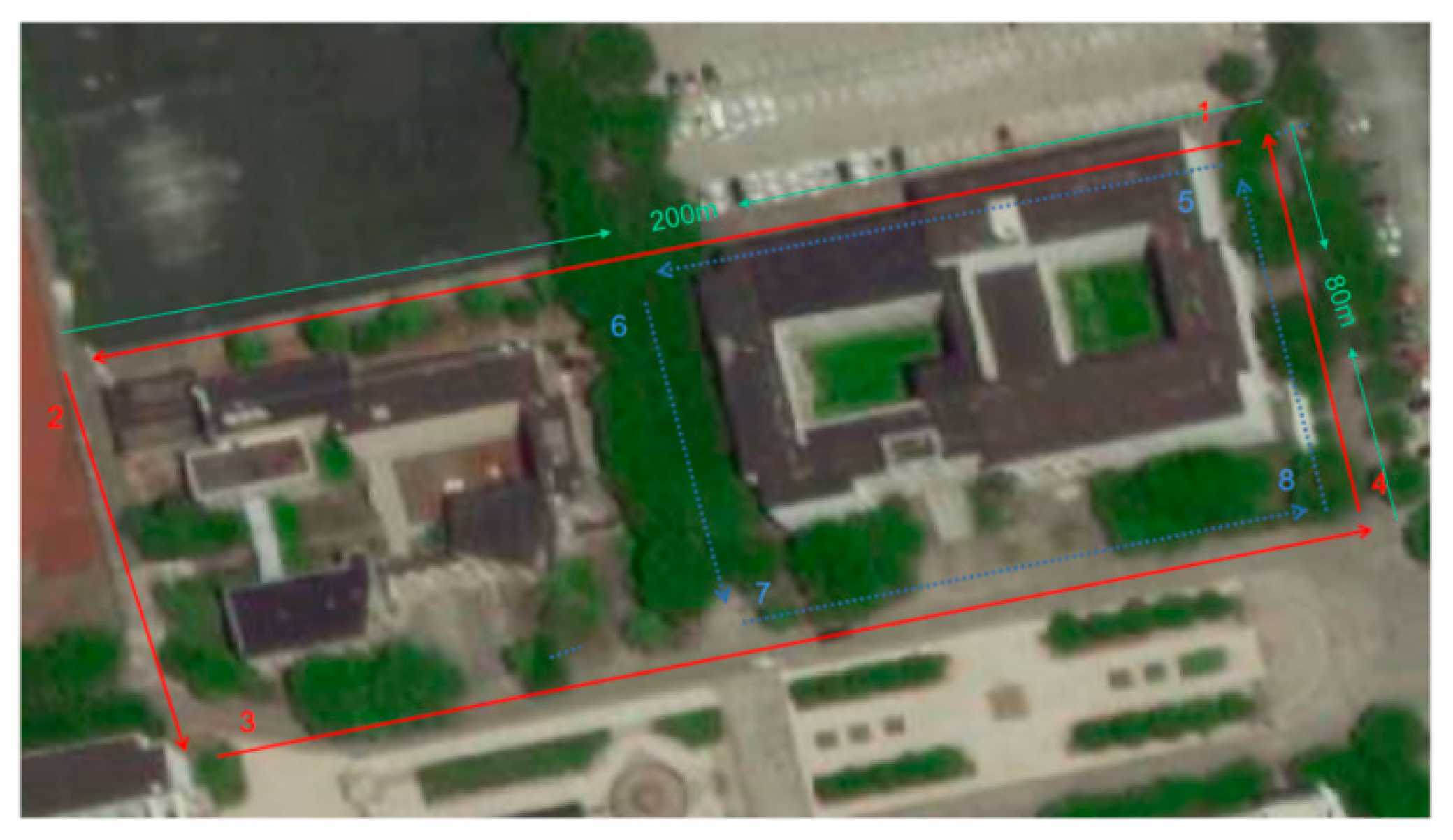
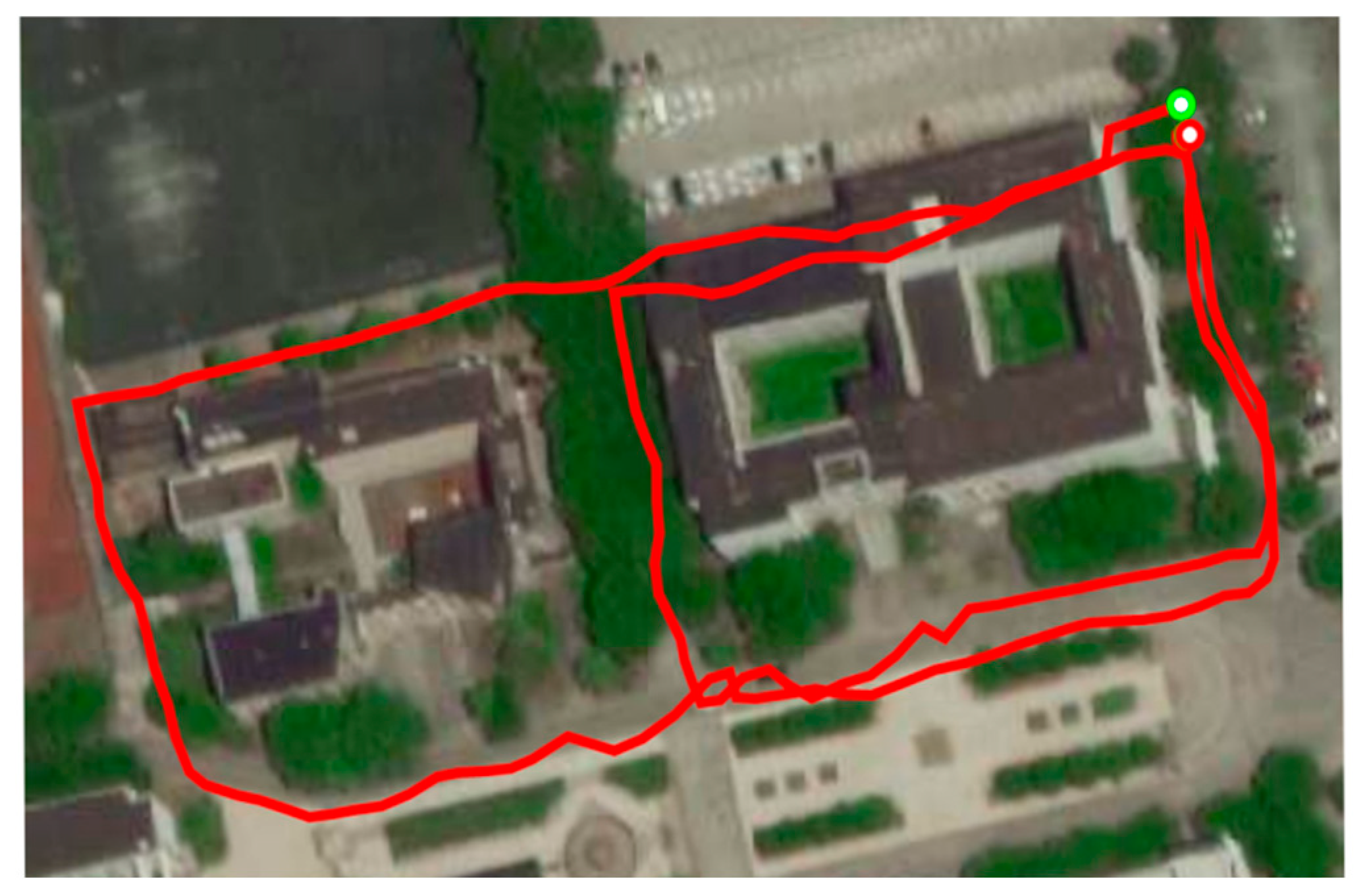
To further verify the performance of the proposed algorithm in outdoor environments, we collected an 8-shaped path around Jingwen Library and Wenhui Building on the east campus of Soochow University. The path sequence was consistent with the number sequence in Figure 11. The trajectory of this scene measured by GPS is shown in Figure 12.

Figure 11.
The 8-shaped path formed around Jingwen Library and Wenhui Building.
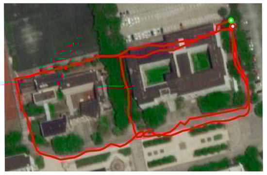
Figure 12.
The ground truth of 8-shaped path formed around Jingwen Library and Wenhui Building.
The data collection occurred at approximately 7 a.m. and lasted for 10 min, during which the loop-closure path had a change in sunlight.
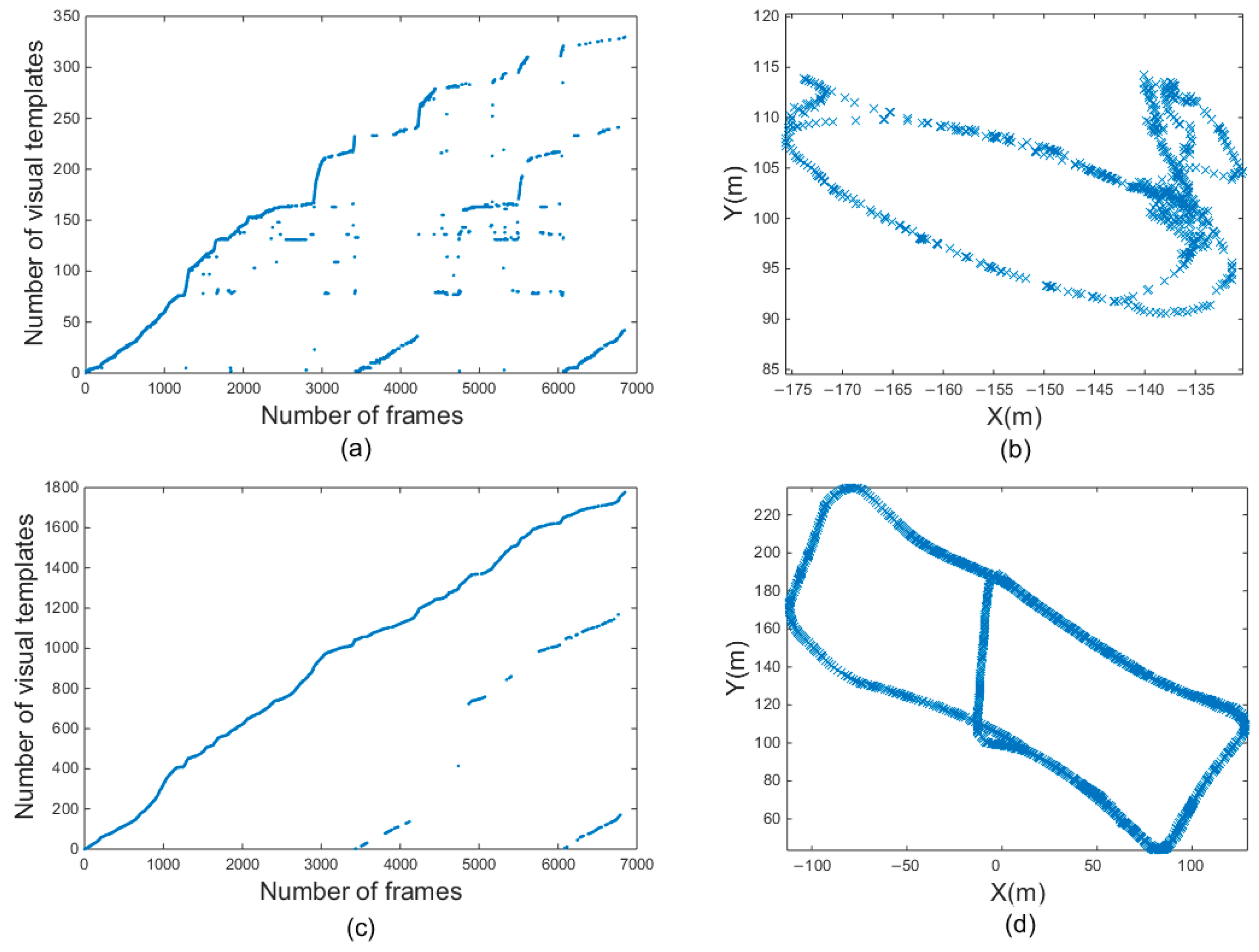
Figure 13a,c are the results of a dataset formed between two buildings. They were obtained using the traditional RatSLAM algorithm and the proposed method, respectively. In fact, real loop closure appears after 3000 frames, so the scattered points before 3000 frames in the visual template obtained by the traditional RatSLAM algorithm are mismatched points. In contrast, the improved algorithm based on the HSI color space had no scattered mismatching points before 3000 frames. It had a higher visual template accuracy.

Figure 13.
Experimental results of the third scene. (a,b) are visual templates and experience map output by traditional RatSLAM. (c,d) are visual templates and experience map output by RatSLAM based on HSI model.
Figure 13b,d are the experience maps of the 8-shaped path formed around two buildings through the original algorithm and the improved algorithm. It can be clearly observed that the experience map shown in Figure 13b is far from the real path. This is because there are too many mismatched points, resulting in many wrong loop-closure corrections, producing a chaotic experience map. In contrast, the number of mismatched experience points by the improved algorithm was substantially reduced, and an accurate experience map could be established, as shown in Figure 13d.
The traditional RatSLAM algorithm could not establish the experience map in third scene as it did in first scene and second scene. This was because the third scene was much larger than first scene and second scene, and the cumulative error in the system kept increasing, which led to an excessive number of visual template mismatches and the reduction of the robustness of the system. The algorithm based on the HSI color space optimized the front-end input of the system, improved the mapping accuracy, and established an experience map in third scene.
4.5.4. Fourth Scene: An Office in the Fusinopolis Building, Singapore
This open dataset was collected in a typical office scene in Singapore and provided by Bo Tian [13].
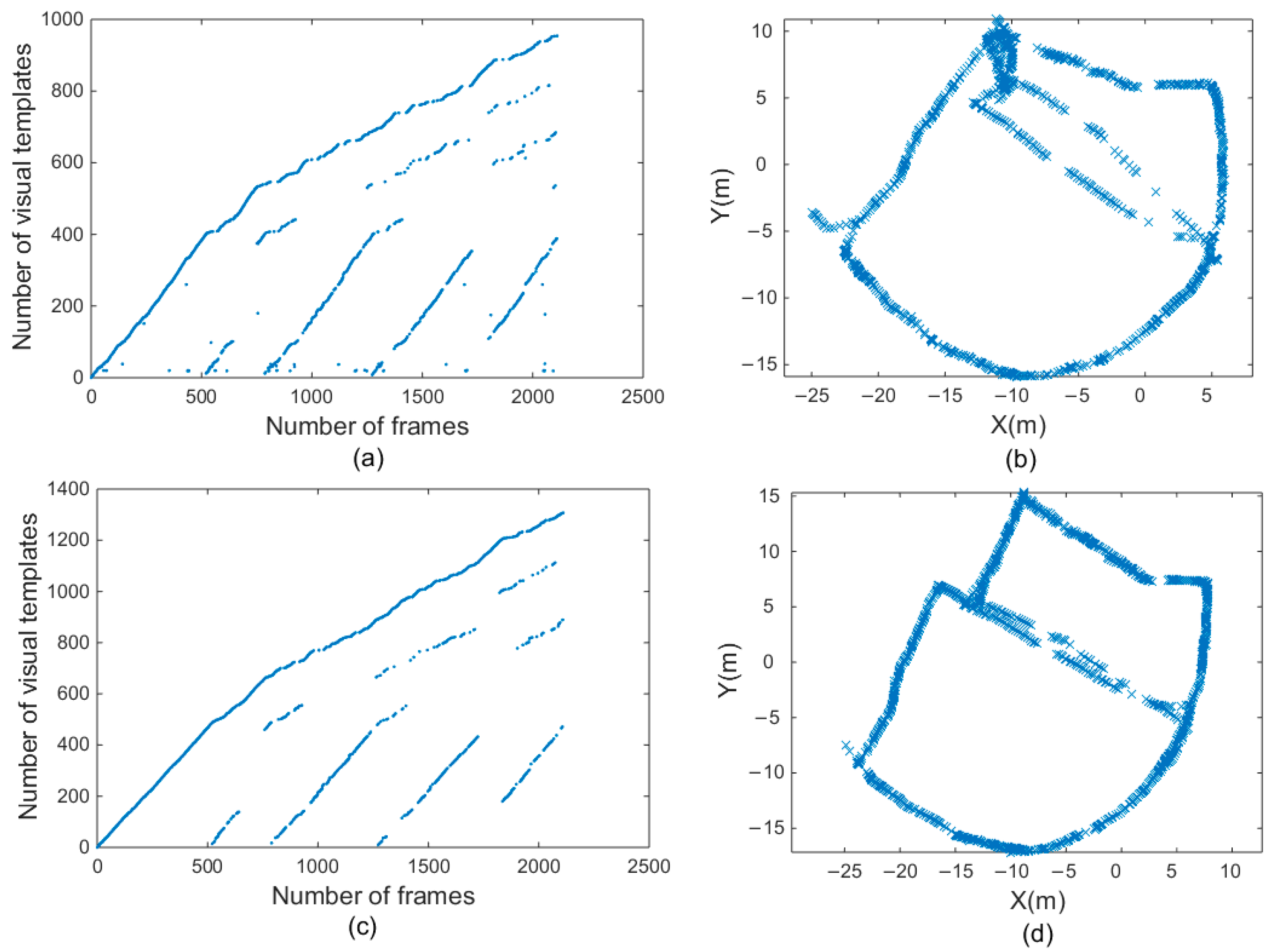
Figure 14a,c illustrate the results of the visual template for office scenes, which were obtained before and after the proposed improvement, respectively. Comparing the two pictures shows that there are more scattered points in Figure 14a. These scattered points are mismatches. When there are too many scattered points, the accuracy of the map deteriorates. The visual templates shown in Figure 14c do not have these scattered points, which means that the number of FPs was reduced, and the number of correct loop closures was greater.
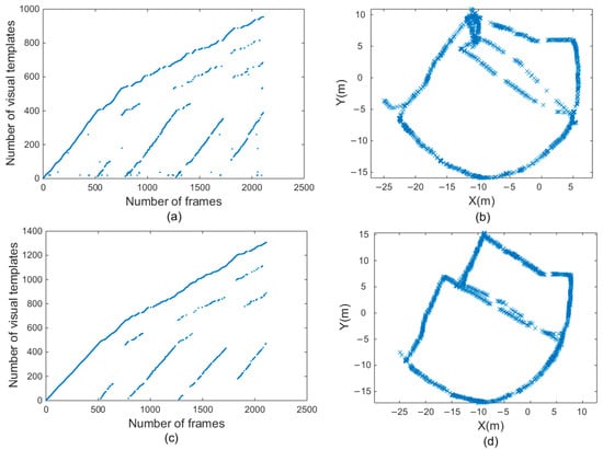
Figure 14.
Experimental results of fourth scene. (a,b) are visual templates and experience map output by traditional RatSLAM. (c,d) are visual templates and experience map output by RatSLAM based on HSI model.
Figure 14b,d show experience maps of the office scene in the open datasets. The original algorithm had a large mapping error. The same path was incorrectly considered as two paths because of the mismatched visual templates. The improved algorithm based on the biological vision model could build a more accurate experience map because the visual template matching accuracy was higher and the number of erroneous loop closures was smaller.
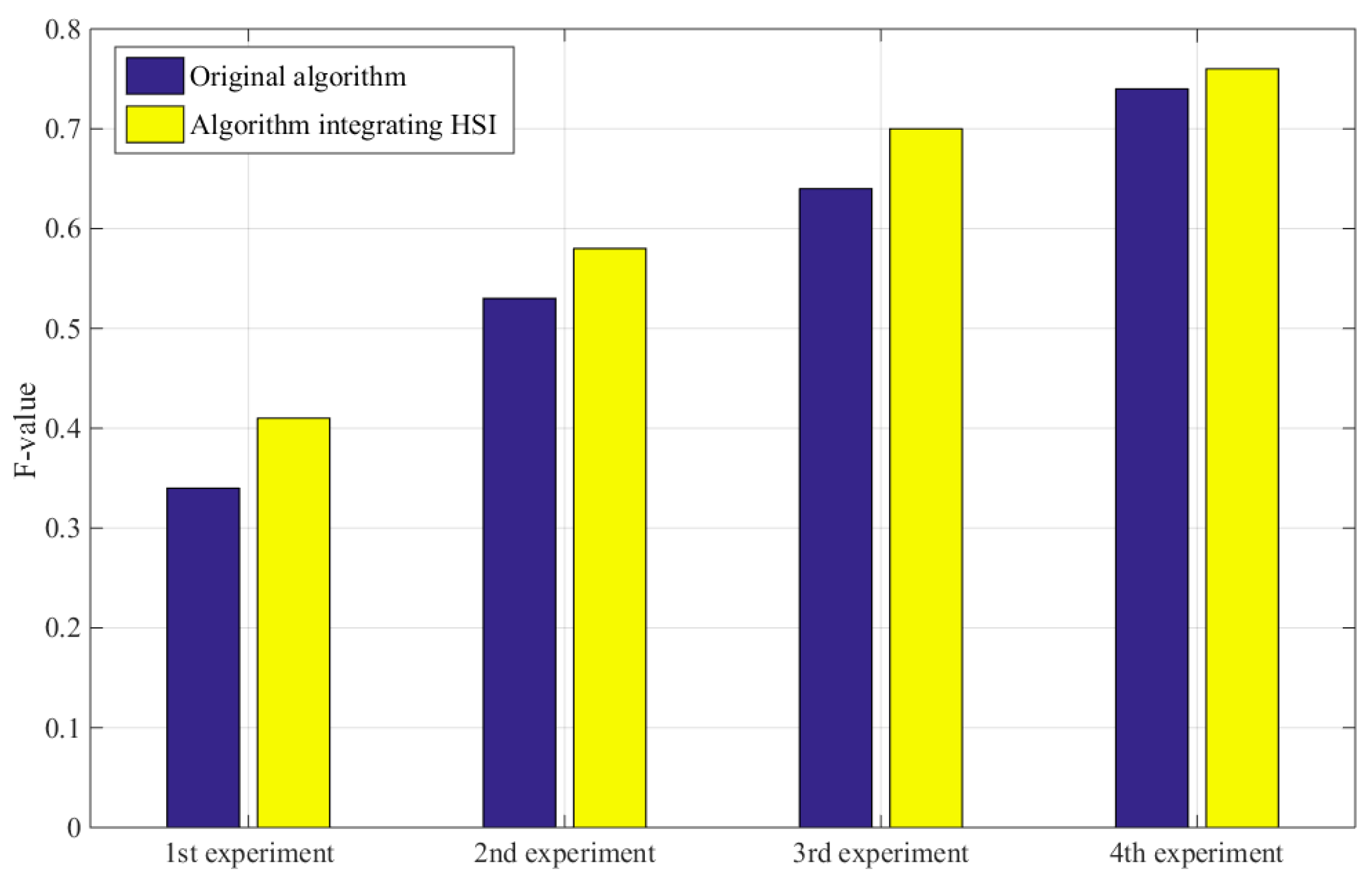
Furthermore, good algorithms should improve the accuracy without reducing recall rates. Table 4 shows that, compared with the original RatSLAM algorithm, the improved method had fewer FPs, and its accuracy and recall rate were superior. The F value is used to comprehensively evaluate the precision rate and recall rate. The higher the F value is, the better the result is. In the first scene and second scene with obvious illumination variation, the method based on the HSI model identified more true-positive loop-closure points and had higher F value than the method based on FT model and traditional RatSLAM. Therefore, in the scene facing varying illumination, the algorithm based on the HSI color space had higher accuracy of mapping and robustness of system. Figure 15 shows the F values of four experiments before and after the improvement. Through comparison, it can be found that the improved method had a higher F value in multiple scenes.
Table 4.
Statistical table of accuracy, recall rate, and F-value.

Figure 15.
Comparison of F values before and after improvement of four experiments.
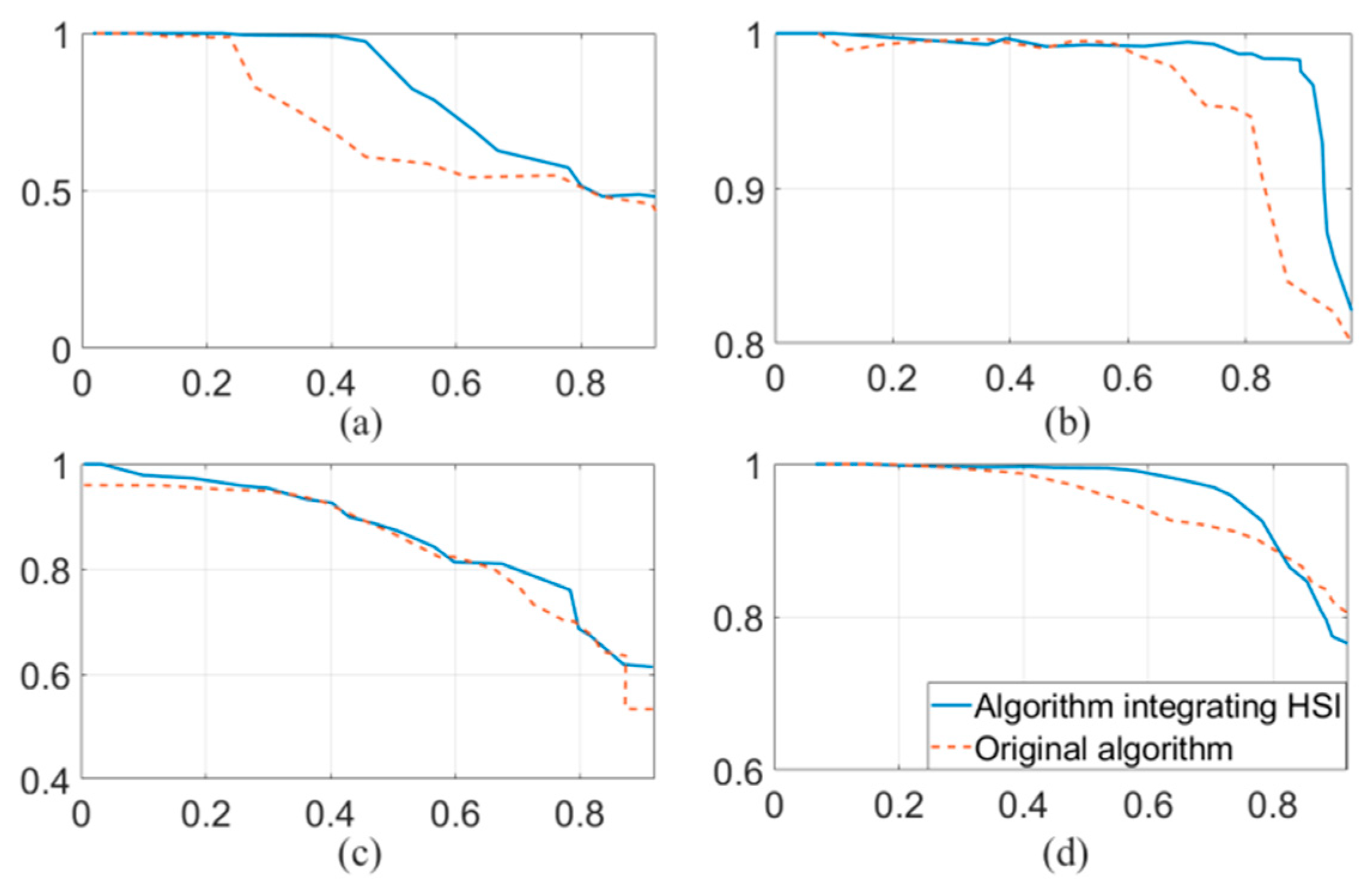
In Figure 16a–d are precision–recall curves of the four experiments. The curves not only reflect the changes in precision rates and recall rates but also show the attributes of the algorithm under different parameters. The blue solid line in the figures indicates the precision–recall curve of the improved algorithm, while the red dashed line indicates the original one. Comparing the two curves shows that the accuracy of the improved method was higher than that before improvement at most recall rates. This result again shows that the improved method had higher robustness and better environmental adaptability.
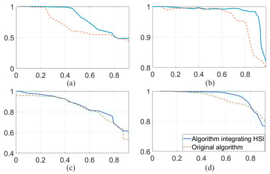
Figure 16.
(a–d) are precision–recall curves of the four experiments, respectively.
5. Conclusions and Future Works
This paper proposed integrating the HSI color space of a biomimetic visual model into a RatSLAM system. A homomorphic filter was adopted to weaken the influence of light intensity. The guided filter was used to reinforce the image details. The results of four experiments showed that the robustness of the visual template, the performance of loop-closure detection, and the environmental adaptability of the entire system obtained great improvements. To test the effectiveness of the biomimetic navigation algorithm fusing the biological vision model, the performance of the proposed algorithm was verified by comparing the accuracy of visual templates generated in different environments and the loop-closure detection of experience maps. The experimental results show that the erroneous visual template matching of the improved method was reduced. The matching of the visual template was not affected when the light changed. The proposed method reinforced the image details, thus increasing the number of TPs and reducing the number of FPs during template matching and finally improving the accuracy of experience maps. The precision–recall curve shows that the proposed method improved the accuracy of loop-closure detection, as well as the robustness and environmental adaptability.
The method proposed in this paper has room for improvement. First, the algorithm contains no correction for the odometer information, which makes the drift increase continuously. Second, the experimental data were collected with a hand-held monocular camera. For biomimetic purposes, a rodent-like robot would be more suitable.
The research on bionic navigation is a way to realize robotic intelligence and make a robot more similar to human beings. Although the current bionic method has defects that need to be rectified, it has great development prospects. The HSI color space pipeline processing technology can also be used to remove fog, which will be conducive to robot navigation in complex environments, such as in fog. In future work, the HSI color space can also be combined with an attention mechanism to realize image detection. This can facilitate the loop-closure detection problem in path planning in space, just as animals store the path information in the form of memory and establish memory associations during navigation.
Author Contributions
Conceptualization, S.Y. and R.S.; methodology, R.S. and L.C.; writing—original draft preparation, C.W. and S.Y.; writing—review and editing, R.S. and L.C.; Experiment and data analysis, C.W. and S.Y. All authors have read and agreed to the published version of the manuscript.
Funding
We received grants from the Joint Fund of Science and Technology Department of Liaoning Province and State Key Laboratory of Robotics of China (no. 2020-KF-22-13) and the National Natural Science Foundation of China (no. 61903341).
Institutional Review Board Statement
Not applicable.
Informed Consent Statement
Not applicable.
Data Availability Statement
Not applicable.
Acknowledgments
We are particularly grateful to Tian from Sichuan University, China, for providing the open dataset that was used as the fourth experiment in our work. Finally, we express our gratitude to all the people and organizations that have helped with this work.
Conflicts of Interest
The authors declare no conflict of interest.
References
- Milford, J.M.; Wyeth, G.F.; Prasser, D. RatSLAM: A hippocampal model for simultaneous localization and mapping. In Proceedings of the IEEE International Conference on Robotics and Automation, New Orleans, LA, USA, 26 April–1 May 2004. [Google Scholar]
- O’Keefe, J. Place units in the hippocampus of the freely moving rat. Exp. Neurol. 1976, 51, 78–109. [Google Scholar] [CrossRef]
- Taube, J.; Muller, R.; Ranck, J. Head-direction cells recorded from the postsubiculum in freely moving rats. I. Description and quantitative analysis. J. Neurosci. 1990, 10, 420–435. [Google Scholar] [CrossRef] [PubMed] [Green Version]
- Hafting, T.; Fyhn, M.; Molden, S.; Moser, M.B.; Moser, E.I. Microstructure of a spatial map in the entorhinal cortex. Nature 2005, 436, 801–806. [Google Scholar] [CrossRef] [PubMed]
- Prasser, D.; Milford, M.; Wyeth, G. Outdoor Simultaneous Localisation and Mapping Using RatSLAM. In Field and Service Robotics; Springer: Berlin/Heidelberg, Germany, 2006; Volume 25, pp. 143–154. [Google Scholar]
- Milford, M.J.; Wyeth, G.F. Mapping a Suburb With a Single Camera Using a Biologically Inspired SLAM System. IEEE Trans. Robot. 2008, 24, 1038–1053. [Google Scholar] [CrossRef] [Green Version]
- Milford, M.J.; Schill, F.; Corke, P.; Mahony, R.; Wyeth, G. Aerial SLAM with a single camera using visual expectation. In Proceedings of the 2011 IEEE International Conference on Robotics and Automation, Shanghai, China, 9–13 May 2011. [Google Scholar]
- Milford, M.; Jacobson, A.; Chen, Z.; Wyeth, G. RatSLAM: Using Models of Rodent Hippocampus for Robot Navigation and Beyond. In Robotics Research; Inaba, M., Corke, P., Eds.; Springer: Cham, Switzerland, 2016; Volume 114. [Google Scholar]
- Glover, A.J.; Maddern, W.P.; Milford, M.J.; Wyeth, G.F. FAB-MAP + RatSLAM: Appearance-based SLAM for multiple times of day. In Proceedings of the 2010 IEEE International Conference on Robotics and Automation, Anchorage, AK, USA, 3–7 May 2010. [Google Scholar]
- Zhou, S.C.; Yan, R.; Li, J.X.; Chen, Y.K.; Tang, H. A brain-inspired SLAM system based on ORB features. Int. J. Autom. Comput. 2017, 14, 564–575. [Google Scholar] [CrossRef] [Green Version]
- Kazmi, S.A.M.; Mertsching, B. Gist+RatSLAM: An Incremental Bio-inspired Place Recognition Front-End for RatSLAM. In Proceedings of the 9th EAI International Conference on Bio-inspired Information and Communications Technologies (formerly BIONETICS), New York, NY, USA, 1 May 2016. [Google Scholar]
- Tubman, R.; Potgieter, J.; Arif, K.M. Efficient robotic SLAM by fusion of RatSLAM and RGBD-SLAM. In Proceedings of the 23rd International Conference on Mechatronics and Machine Vision in Practice (M2VIP), Nanjing, China, 28–30 November 2017. [Google Scholar]
- Tian, B.; Shim, V.A.; Yuan, M.; Srinivasan, C.; Tang, H.; Li, H. RGB-D based cognitive map building and navigation. In Proceedings of the 2013 IEEE/RSJ International Conference on Intelligent Robots and Systems, Tokyo, Japan, 3–7 November 2013. [Google Scholar]
- Salman, M.; Pearson, M.J. Advancing whisker based navigation through the implementation of Bio-Inspired whisking strategies. In Proceedings of the 2016 IEEE International Conference on Robotics and Biomimetics (ROBIO), Qingdao, China, 3–7 December 2016. [Google Scholar]
- Milford, M.; McKinnon, D.; Warren, M.; Wyeth, G.; Upcroft, B. Feature-based Visual Odometry and Featureless Place Recognition for SLAM in 2.5 D Environments. In Proceedings of the Australasian Conference on Robotics and Automation, Melbourne, Australia, 7–9 December 2011. [Google Scholar]
- Silveira, L.; Guth, F.; Drews, P., Jr.; Ballester, P.; Machado, M.; Codevilla, F.; Duarte-Filho, N.; Botelho, S. An Open-source Bio-inspired Solution to Underwater SLAM. In Proceedings of the 4th IFAC Workshop on Navigation, Guidance and Control of Underwater Vehicles (NGCUV) 2015, Girona, Spain, 28–30 April 2015; Elsevier: Amsterdam, The Netherlands, 2015. [Google Scholar]
- Ball, D.; Heath, S.; Milford, M.; Wyeth, G.; Wiles, J. A navigating rat animat. In Proceedings of the 12th International Conference on the Synthesis and Simulation of Living Systems, Odense, Denmark, 19–23 August 2010; MIT Press: Cambridge, MA, USA, 2010; pp. 804–811. [Google Scholar]
- Milford, M.; Schulz, R.; Prasser, D.; Wyeth, G.; Wiles, J. Learning spatial concepts from RatSLAM representations. In Robotics and Autonomous Systems; Elsevier: Amsterdam, The Netherlands, 2007; Volume 55, pp. 403–410. [Google Scholar]
- Qin, G.; Xinzhu, S.; Mengyuan, C. Research on Improved RatSLAM Algorithm Based on HSV Image Matching. J. Sichuan Univ. Sci. Eng. 2018, 31, 49–55. [Google Scholar]
- Fan, C.N.; Zhang, F.Y. Homomorphic filtering based illumination normalization method for face recognition. Pattern Recognit. Lett. 2011, 32, 1468–1479. [Google Scholar] [CrossRef]
- Nnolim, U.; Lee, P. Homomorphic Filtering of colour images using a Spatial Filter Kernel in the HSI colour space. In Proceedings of the 2008 IEEE Instrumentation and Measurement Technology Conference, Victoria, BC, Canada, 12–15 May 2008; pp. 1738–1743. [Google Scholar]
- Ball, D.; Heath, S.; Wiles, J.; Wyeth, G.; Corke, P.; Milford, M. OpenRatSLAM: An open source brain-based SLAM system. Auton. Robot. 2013, 34, 149–176. [Google Scholar] [CrossRef]
- Milford, M.J. Robot Navigation from Nature: Simultaneous Localisation, Mapping, and Path Planning Based on Hippocampal Models; Springer Science & Business Media: Berlin, Germania, 2008; Volume 41. [Google Scholar]
- Milford, M. Vision-based place recognition: How low can you go? Int. J. Robot. Res. 2013, 32, 766–789. [Google Scholar] [CrossRef]
- Townes-Anderson, E.; Zhang, N. Synaptic Plasticity and Structural Remodeling of Rod and Cone Cells. In Plasticity in the Visual System; Springer: Boston, MA, USA, 2006. [Google Scholar]
- Dhandra, B.V.; Hegadi, R.; Hangarge, M.; Malemath, V.S. Analysis of Abnormality in Endoscopic images using Combined HSI Color Space and Watershed Segmentation. In Proceedings of the 18th International Conference on Pattern Recognition (ICPR'06), Hong Kong, China, 20–24 August 2006. [Google Scholar]
- Ju, Z.; Chen, J.; Zhou, J. Image segmentation based on the HSI color space and an improved mean shift. In Proceedings of the Information and Communications Technologies (IETICT 2013), Beijing, China, 27–29 April 2013. [Google Scholar]
- Gonzalez, R.C.; Woods, R.E. Digital Image Processing, 2nd ed.; Prentice Hall: New York, NY, USA, 2003. [Google Scholar]
- Yang, H.; Wang, J. Color Image Contrast Enhancement by Co-occurrence Histogram Equalization and Dark Channel Prior. In Proceedings of the 2010 3rd International Congress on Image and Signal Processing, Yantai, China, 16–18 October 2010. [Google Scholar]
- Blotta, E.; Bouchet, A.; Ballarin, V.; Pastore, J. Enhancement of medical images in HSI color space. J. Phys. Conf. 2011, 332, 012041. [Google Scholar] [CrossRef]
- Guo, Y.; Zhang, Z.; Yuan, H.; Shao, S. Single Remote-Sensing Image Dehazing in HSI Color Space. J. Korean Phys. Soc. 2019, 74, 779–784. [Google Scholar] [CrossRef]
- Dong, S.; Ma, J.; Su, Z.; Li, C. Robust circular marker localization under non-uniform illuminations based on homomorphic filtering. Measurement 2020, 170, 108700. [Google Scholar] [CrossRef]
- Delac, K.; Grgic, M.; Kos, T. Sub-Image Homomorphic Filtering Technique for Improving Facial Identification under Difficult Illumination Conditions. In Proceedings of the International Conference on Systems, Signals and Image Processing, Budapest, Hungary, 21–23 September 2006. [Google Scholar]
- Frezza, F.; Galli, A.; Gerosa, G.; Lampariello, P. Characterization of the resonant and coupling parameters of dielectric resonators of NRD-guide filtering devices. In Proceedings of the 1993 IEEE MTT-S International Microwave Symposium Digest, Atlanta, GA, USA, 14–18 June 1993. [Google Scholar]
- Jiang, H.; Zhao, Y.; Gao, J.; Gao, Z. Adaptive pseudo-color enhancement method of weld radiographic images based on HSI color space and self-transformation of pixels. Rev. Sci. Instrum. 2017, 88, 065106. [Google Scholar] [CrossRef] [PubMed]
- Lu, B.; Chen, J.; Zheng, Y.; Wang, J. Tone mapping algorithm of iCAM06 based on guide filtering. Opt. Tech. 2016, 42, 130–135,140. [Google Scholar]
- Biswas, P.; Pramanik, S.; Giri, B.C. Cosine Similarity Measure Based Multi-attribute Decision-making with Trapezoidal Fuzzy Neutrosophic Numbers. Neutrosophic Sets Syst. 2015, 8, 47–56. [Google Scholar]
- Yu, S.; Wu, J.; Xu, H.; Sun, R.; Sun, L. Robustness Improvement of visual templates Matching Based on Frequency-Tuned Model in RatSLAM. Front. Neurorobotics 2020, 14, 568091. [Google Scholar] [CrossRef] [PubMed]
- Ma, L.; Zhang, C. Optimization design of homomorphic Filter based on Matlab. Appl. Opt. 2010, 4, 584–588. [Google Scholar]
- Ling, G.; Zhang, Q. Image Fusion Method Combining Non-subsampled Contourlet Transform and Guide Filtering. Infrared Technol. 2018, 40, 444–448. [Google Scholar]

Publisher’s Note: MDPI stays neutral with regard to jurisdictional claims in published maps and institutional affiliations. |
© 2022 by the authors. Licensee MDPI, Basel, Switzerland. This article is an open access article distributed under the terms and conditions of the Creative Commons Attribution (CC BY) license (https://creativecommons.org/licenses/by/4.0/).