Abstract
Currently, interest in deep learning-based semantic segmentation is increasing in various fields such as the medical field, automatic operation, and object division. For example, UNet, a deep learning network with an encoder–decoder structure, is used for image segmentation in the biomedical area, and an attempt to segment various objects is made using ASPP such as Deeplab. A recent study improves the accuracy of object segmentation through structures that extend in various receptive fields. Semantic segmentation has evolved to divide objects of various sizes more accurately and in detail, and various methods have been presented for this. In this paper, we propose a model structure that reduces the overall parameters of the deep learning model in this development and improves accuracy. The proposed model is an encoder–decoder structure, and an encoder half scale provides a feature map with few encoder parameters. A decoder integrates feature maps of various scales with high area details and forward features of low areas. An integrated feature map learns a feature map of each encoder hierarchy over an area of previous data in the form of a continuous coupling structure. To verify the performance of the model, we learned and compared the KITTI-360 dataset with the Cityscapes dataset, and experimentally confirmed that the proposed method was superior to the existing model.
1. Introduction
The semantic segmentation task is to label all pixels in the image as belonging to one of the N classes. It aims to perform dense-prediction to label each pixel of the image. In the case of semantic segmentation with this goal, various models have been proposed. However, excellent semantic segmentation, which requires class information in the pixel region, cannot be achieved using the classical CNN structure [1] for the following reasons.
- In general CNNs, spatial details are lost owing to the pooling of pixel semantic information in deep layers and the stride of the filters.
- The presence of several objects of different sizes in an image requires processing of various sizes, which increases the computational complexity.
- The spatial pooling of CNNs affects the location accuracy of pixels.
The categories of CNN can be divided into various application fields and methods [2]. We focused on the network structure of semantic segmentation techniques.
The fully convolutional network (FCN) [3] is a structure that significantly improves the accuracy of semantic segmentation beyond that of classical CNN structures. It is the basis of semantic segmentation technology. The FCN incorporates an up-sampling step and skip-connection strategy into a general CNN structure to increase the semantic accuracy. The skip-connection strategy compensates for information loss in the pooling process of the CNN using the feature maps in the intermediate stage.
SegNet [4] uses the backbone of a CNN called VGG16 and has a segmentation network composed of an encoder and decoder. This structure is also frequently used in recent models. The decoder stages of this structure have computational efficiency because they use indices in the maximum pooling stage of the encoder.
U-Net [5] uses a skip-connection strategy based on an encoder–decoder structure to solve the problem of model accuracy and information loss. It is widely used for the semantic segmentation of medical images, and various approaches to improve the performance of U-Net have been proposed [6,7].
The DeepLab model [8,9,10] simultaneously enhances the computational speed, accuracy, and simplicity of the structure; it is based on atrous convolution, which is widely used in the communication field. Therefore, information on a wide range of feature maps can be obtained without additional parameters or calculations. In addition, the conditional random field [11] and atrous spatial pyramid pooling (ASPP) [9] have been applied for improved accuracy and computational efficiency for processing multiple scales.
Recently, CNN structures for semantic segmentation have been applied in the autonomous driving field. Levi [12] proposed a CNN structure that was an improvement on the traditional CNN for obstacle and road segmentation.
In Oliveira [13], a method to increase computational efficiency by changing the classical FCN structure for road and lane segmentation was proposed. The model achieved this improvement by applying the pooling layer of the contractive side to the up-convolutional network of the FCN. Romera [14] proposed a new CNN structure (ERFNet) that considers both accuracy and computational accuracy in solving the image segmentation problem in AVs. Pizzati [15] adopted the ERFNet structure and an additional decoder layer to detect lanes and free space. Scheck [16] proposed a method to detect free spaces using a single omnidirectional camera with a fisheye lens, and the accuracy was compared with that of the FCN-based encoder-decoder method and DeepLabv3. Hou [17] presented a lightweight CNN structure for lane detection. In this structure, E-Net [18], one of the ResNet series and encoder–decoder structures, was adopted as the backbone. Self-attention distillation, a novel knowledge distillation approach, was proposed to solve the computational complexity. Chan [19] presented a new instance segmentation method that combines an advanced FCN and inverse perspective mapping (IPM) [20] technology to simultaneously mark lanes and detect drivable areas. Segmentation was performed using the FCN. The IPM technology has also been adopted for lane and obstacle recognition. [21] used ResNet18 [22] as a backbone and achieved a fast frame rate by learning only the boundary of the drivable area. Qiao [23] proposed a method to analyze the scenes of AVs and predict the drivable area using a deep learning structure (DeepLabv3) with an encoder–decoder network. ResNet101 was used as the backbone. The atrous spatial pyramid pooling (ASPP) module was added to the last encoder layer to collect context and semantic information.
Based on the above-mentioned content, the research focus of semantic segmentation technology is as follows.
- (1)
- Improved CNN structure to effectively segment objects of varying sizes
- (2)
- Structural design with fewer parameters than other models
- (3)
- Parameter sharing and high performance through a structure that delivers a variety of reactive fields
In this study, we propose a new encoder–decoder-based semantic segmentation technique that combines multilayer(ML)-ASPP and a two-step cross-stage, which has the advantage of fast operation. The proposed model applies a new process called multilayer ASPP (ML-ASPP) to obtain more contextual information after the last convolution operation of the encoder. The classical ASPP is applied only to a single feature map, whereas the ML-ASPP performs ASPP using all the layers of the encoder to obtain more diverse and contextual information. In addition, another new technique, two-step cross-stage (TS-CS), was used for the encoder and decoder to increase the computational efficiency. The application of these two operations rendered the proposed model superior to the classical methods in terms of the learning parameters and operation speed. The proposed model was tested using the KITTI-360 2D segmentation dataset [24] and cityscapes dataset (including high-noise data) [25] for performance evaluation, and its performance was compared and analyzed with those of other methods.
2. Related Research
Figure 1, Figure 2 and Figure 3 show a brief overview of each structure for each version of UNet [5,6,7]. UNet3+ features a redesigned skip connection that is different from that of UNet and UNet++, and uses full-scale deep supervision to combine layers of various sizes. The output is used to distinguish between accurate location recognition and boundaries with fewer parameters.
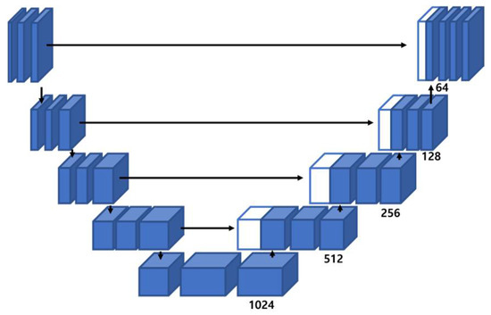
Figure 1.
Structure of UNet model [5].
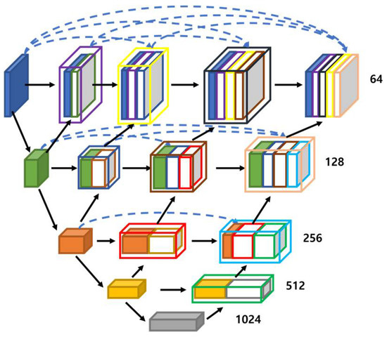
Figure 2.
Structure of UNet++ model [7].
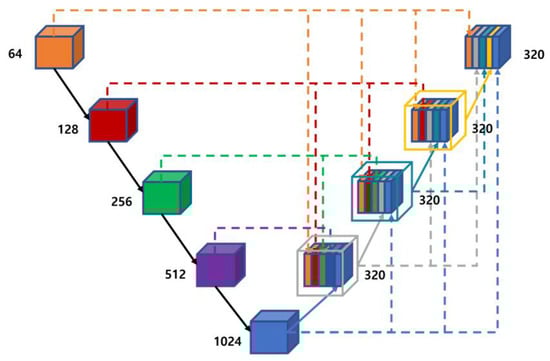
Figure 3.
Structure of UNet3+ model [6].
UNet is used for medical image segmentation and has an encoder–decoder transformation structure. It uses skip connections to combine various information in the decoder with the same feature map and the corresponding sublevel feature map in the encoder. The skip connection used by the UNet is shown in Figure 1.
The UNet++ model features a nested and dense skip connection, which overlaps features for each layer and has a high number of channels to enhance the connection to each layer. This aims to reduce the difference in the feature-related information between the encoder and decoder. Although UNet++ also exhibits good performance, the number of parameters increases to contain all the corresponding information. UNet3+ features a structure to contain all the feature information of the entire input, as shown in Figure 3.
To address the segmentation problem, the location information corresponding to the input image must be preserved. UNet3+ outperforms the previous UNet models owing to its full-scale skip connection, which carries information corresponding to each encoder layer, thus preventing location information loss.
Studies on the DeepLab network suggest that semantic segmentation should infer situations of various sizes [8,9,10]. DeepLabv1 v2 has raised doubts about regarding the process of extracting image features and restoring the downsampled image to its original size. Based on this suspicion, location information could be lost in the case of a structure without a skip connection, such as UNet, and the encoder–decoder structure was eliminated. In DeepLabv2, in place of the encoder–decoder structure, the results were derived through atrous convolution, as shown in Figure 4.
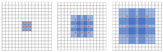
Figure 4.
Atrous convolution [9].
Atrous convolution was used for two reasons. First, it increases the receptive field. Second, various sizes can be responded to by adjusting the dilation parameters. This can be exploited to reduce the number or size of the pooling layers to cover a wide receptive field with the same number of filters, thereby reducing the overall number of parameters. The DeepLab model uses atrous convolution. The structure of each model is shown in Figure 5 and Figure 6, respectively.
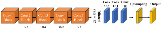
Figure 5.
Structure of DeepLabv1 model.
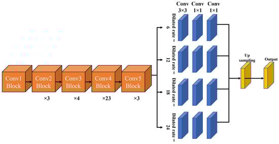
Figure 6.
Structure of DeepLabv2 model.
The pyramid pooling layer proposed by PSPNet [26] underscores the difference between v1 and v2. In PSPNet, the dilation rates are 1, 2, 3, and 6, thus forming a sub-region. In v2, the configuration is repaired by adjusting the dilation rate to a multiple of six, as shown in Figure 6; furthermore, a pyramid pooling layer with receptive fields of various sizes is configured, owing to which it outperforms the previous DeepLab v1.
The global average pooling used in PSPNet is incorporated into DeepLab v3 [10] as Figure 7, and the structure is changed through concatenation based on the method of summing in v2. The changed structure allows it to retain its receptive field, and 1 × 1 and 3 × 3 convolutions are applied in parallel with different dilation rates, 6, 12, 18, 12, 24, and 36. In addition, global average pooling is applied to understand the global context. For DeepLabv3, an experiment was conducted by varying the dilation rate ratio from block4 to 7.
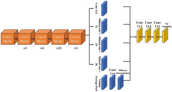
Figure 7.
Structure of DeepLabv3 model.
Numerous of the aforementioned models apply various techniques to obtain more meaningful information in feature maps of multiple sizes. These studies attempted to find coarse or detailed information about classes in high-resolution and low-resolution feature maps. Segmentation research is aimed at enhancing and segmenting the boundaries of individual classes in an image by extracting the location of information, such as class boundaries, from high-resolution feature maps. However, as the feature maps are transferred layer wise, information on the image is diluted and lost owing to down sampling.
These problems can be solved by combining spatial and semantic information with resolutions of various sizes.
3. Proposed Method
In this section, we describe the overall structure of the proposed system. Figure 8 shows the CNN structure with the proposed ML-ASPP and TS-CS. The proposed structure adopts an encoder and decoder-based CNN structure. It has an ML-ASPP, which transmits various resolution information to the decoder layer using the feature maps of all layers in the encoder. In addition, in the ML-ASSP, the input and output feature maps differ according to the corresponding decoder layer, and the outputs are concatenated.
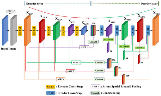
Figure 8.
The Structure of the proposed CNN with multi-layer ASPP and TS-CS.
The TS-CS is divided into encoder cross-stage (CS-EN) and decoder cross-stage (CS-DE), and the inputs of the CS-EN and CS-DE are composed of different feature maps. The TS-CS achieves high computational efficiency by applying a method similar to skip connections in the generation of feature maps of each layer in the encoder and decoder. Based on these two new methods, the proposed system has fewer network parameters and greater object semantic segmentation accuracy. The details of each process are described in the following subsections.
3.1. CS-EN
In the case of a CNN designed as a deep network for greater accuracy, various disadvantages exist in the transmission and learning of the gradient information. To solve this problem, ResNet [22] applies the shortcut connection structure to prevent the gradient problem and to increase accuracy by creating a deep learning structure with a deeper structure. However, with this structure, the computational complexity increases significantly owing to the presence of many parameters. To solve these shortcomings, DenseNet [27] and CSPNet [28], which can simultaneously increase the operation speed and accuracy, have been proposed.
The DenseNet has a structure in which the input of the dense layer is concatenated with the output, as shown in Figure 9a. This increases the efficiency of the information and gradient flow. However, the gradient information in the back-propagation process for learning tends to overlap.
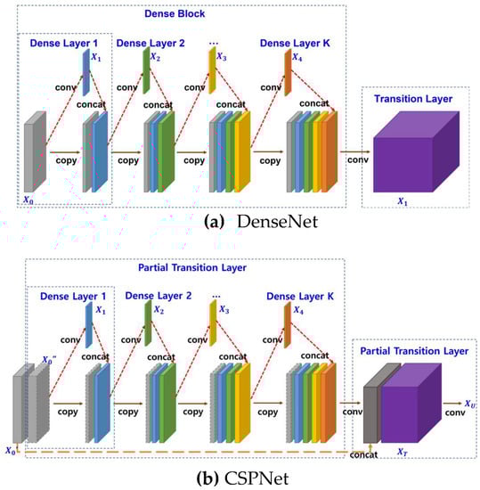
Figure 9.
Structures of DenseNet and CSPNet (CSP-DenseNet).
The CSPNet, which was proposed to solve this problem, adopted the convolution method by dividing the output of the previous layer, as shown in Figure 9b. Its advantage is that it can be applied without changing the backbone structure of most classical CNNs. Equations (1) and (2) are used to update the gradient during the layer feedforward calculation and backpropagation of the DenseNet and CSPNet, respectively.
where is the output of each layer and is the weight of forward pass.
Equations (1) and (2) reveal a significant overlapping gradient information in the backpropagation process of the DenseNet. The overlap increases as the number of dense layers increases.
However, the CSPNet prevents excessive copying of gradient information by dividing the feature map of the base layer into two parts:. The two divided parts have two passes of gradient flow, and the gradient of that does not pass through the dense layer is not copied. Therefore, the CSPNet has greater computational efficiency compared with the DenseNet owing to the reduction in the number of learned parameters.
In this study, we proposed a novel encoder–decoder CNN structure for semantic segmentation inspired by the CSPNet. In the classical semantic segmentation model, only the encoder and corresponding decoder are connected, and adjacent layers are connected. However, in this structure, transmitting detailed information, such as the location and boundary of the class region of the input, to the decoder is challenging. To solve this problem, we proposed a structure that effectively transmits the information of the feature map in each encoder layer and simultaneously lowers the computational complexity. The proposed encoder structure is shown in Figure 10.
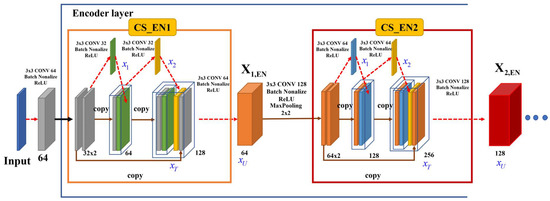
Figure 10.
Proposed CS_EN.
In Figure 8, CS_EN1 represents the cross-stage block of the first encoder layer and represents the output of this block. The input image feature map was divided into two 32-channel feature maps and calculated in the cross stage. The number of convolutions in the cross-stage block can be determined by the designer or the user as a hyperparameter.
The purpose of the cross-stage block at the encoder stage in the proposed method is to preserve as much of the spatial information of the main pixels as possible and reduce the total amount of computation. Therefore, in this study, convolution in the cross-stage block of the encoder was set as . The output of the proposed system and update of the gradient in each layer are as follows:
As can be seen in Equation 3, the overlap of gradient information and parameters in the proposed method are small compared with the DenseNet and CSP-DenseNet.
3.2. ML-ASPP
In classical deep convolution, the resolution of the output result is lower than that of the input data. The feature map with reduced resolution owing to max-pooling and downsampling operations reduces the computational complexity of the CNN and obtains the semantic information of more areas of the feature map.
However, low-resolution feature maps lose the details of valid information, such as boundaries in the field of semantic segmentation. In addition, the same object can exist at different sizes in the image. To compensate for these problems, an ASPP structure that can be applied when classes exist in different sizes in an image was proposed. Figure 11a shows the ASPP applied to the classical CNN and Figure 11b shows the ASPP applied to the encoder-decoder structure.
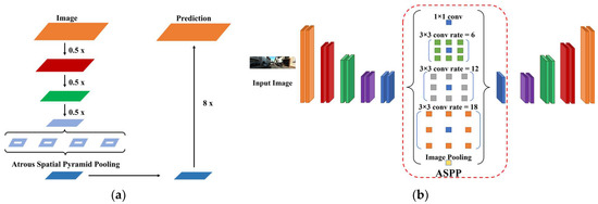
Figure 11.
CNN with ASPP. (a) Classical CNN structure, (b) encoder–decoder CNN structure.
As shown in Figure 11b, the classical ASPP model was operated only once at the end of the encoder of the decoder–encoder model. We devised a method for transmitting semantic information more effectively using the proposed structure. Figure 12 shows the proposed ASPP technique.
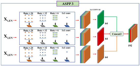
Figure 12.
ML-ASPP in the encoder.
To explain the structure of the proposed algorithm, ASPP3, shown in Figure 8, was used. The method used the multilayer feature map of the encoder to deliver semantic information to the decoder layer. Consequently, the semantic information for various classes was fed into the decoder.
In general, the ASPP output y, the output of the pixel, is given by Equation (4).
where the atrous rate determines the spacing between kernel points. , , and represent the input, position index of the filter, and kth value in the convolution filter, respectively. In this study, the ASPP rates were set at 24, 12, 6, and 1. If the size of the filter was 3 × 3 and was expressed as a one-dimensional index, was displayed from 1 to 9. Using Equation (4) to express the output for each rate, Equation (5) was obtained:
Therefore, the output of atrous convolution for each input can be expressed by the following Equation (6).
where denotes the j th encoder layer; [] denotes a concatenation combination; and is a convolution operation. Using Equations (5) and (6), the output for the ASPPs proposed in this study is expressed as Equation (7):
The proposed method performed ASPP four times over the entire structure, and the computational complexity was greater than that of the existing methods. However, the proposed ML-ASPP delivered semantic information to the decoder more effectively, and the increased computational complexity was reduced in the cross-stage block of the encoder and decoder. Therefore, the proposed method increased the computational complexity of the ASPP but improved the semantic segmentation performance and reduced the required computation for the entire system compared with other classical CNNs.
3.3. Decoder Cross-Stage (CS-EN)
In the decoder layer of the proposed structure, each encoder layer received the extracted feature map through the ASPP. In the case of the feature map obtained through the ASPP, the outputs obtained through the convolution operation () in each encoder layer were concatenated and delivered to the decoder.
Figure 13 shows the structure of the proposed decoder. The first layer of the decoder used only the feature maps of the ASPP block of the encoder layer. The next decoder layer performed the cross-stage using the feature maps that concatenated the feature maps of the previous decoder layer calculated through bilinear interpolation and the output feature maps from the ASPP of the encoder layers.
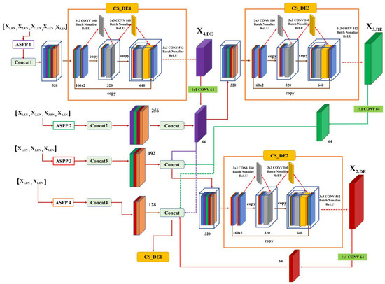
Figure 13.
Structure of the decoder cross-stage (CS-EN).
The combined feature maps of the encoder and decoder had the same resolution, to match the number of channels and reduce unnecessary information. The structure preserved the overall characteristics of the previous layers and successfully retained details, even in operations that changed the scale. Using Equations (6) and (7), each decoder input feature map is expressed as follows:
where F represents the input feature map of each decoder layer, and [ ] denotes the input in the cross-stage block of each decoder.
The decoder cross-stage block performed convolution by dividing the input feature map F into two blocks. Therefore, as in the encoder part of the proposed model, increases in the amount of computational complexity and transmission of excessive gradient information were prevented in the decoder part, and the semantic segmentation performance was improved by merging detailed and coarse information. In addition, in the decoder layer of this method, the parameters of the overall structure were minimized by fixing the number of channels of the final output. In CS-EN, 320 filters, batch normalization, and ReLU functions were used.
3.4. Loss Function and Hyper Parameter
Focal loss [29], Intersection over Union (IoU) loss [30], and MS-SSIM [31] were adopted to learn feature maps of various sizes. Focal loss was adopted to address the class imbalance problem caused by cross-entropy loss. It increases the learning performance by assigning greater weights to cases that are difficult to classify. IoU loss was adopted to improve the performance of the actual label and the predicted result in semantic segmentation. The last layer of the decoder step was calculated as a bilinear, upsampling, and atrous convolution. To accurately distinguish the regions of each object, we used the structural similarity index measure (SSIM) [32] loss function, a multi-scale structure similarity index that assigns higher weights to unclear boundaries. For the proposed model, the regional distribution difference was directly proportional to the MS-SSIM value, which can help eliminate unclear boundaries. Two patches of corresponding size were split in the correct label mask G (ground truth) and P (Prediction), the result of segmentation. The SSIM function is expressed as follows (9):
The multi-scale SSIM function is expressed as Equation (10) below.
where is the prediction and is the label. Finally, the MS-SSIM loss function is given by Equation (11):
where represents the total number of sizes; and represent the averages of and , respectively; and represent the standard deviations of and , respectively; represents the covariance of and ; and and represent the importance of each set scale. In addition, , were set to small values to exclude situations that were divided by zero. M was set to 5, based on a previous study [31]. For the loss function, a three-step segmentation loss function was applied by combining the focal loss function, MS-SSIM loss function, and IoU loss function.
Table 1 shows hyperparameters for models. The size of the model’s input image is fixed at 512 × 256, and the output image also maintains the same size. The dilated ratios of the pyramid pooling layer were fixed at 0, 6, 12, and 18. The experiment was conducted by designating the batch size as 32 and the epoch as 50. The initial learning rate was fixed at 0.01.

Table 1.
Hyperparameters for models.
4. Result and Discussion
4.1. Datasets and Experimental Environments
4.1.1. KITTI-360 Dataset
The proposed method was validated based on the dataset proposed by KITTI-360. The KITTI-360 dataset contains more than 320,000 images and 100,000 laser scans at a mileage of 73.7 km. A dataset with annotation of 3D scenes and instance annotation of point cloud data and 2D images was recorded in the suburbs of Karlsruhe, Germany. In this study, an image was used as illustrated in Figure 12, and the resolution of the original image was adjusted according to the input network size. The original image size of the dataset used was 1408 × 376, and the image resolution was set to 512 × 256 pixels according to the network size. The number of images in the dataset used was 61,058, and the number of segmentation labels corresponding thereto was the same. To learn the proposed network structure, a training dataset and a validation dataset were generated at a ratio of 9:1. The test data were calculated for each model based on the learning results of each model and compared. The equipment used for learning were the Intel i9 CPU, RTX3090ti GPU, and 128 GB RAM.
Figure 14 shows the histogram of the frequency of each class in the KITTI-360 dataset. The KITTI-360 dataset has a total of 33 classes. We analyzed the classes and selected only 12 valid classes. In this study, the performance of each model was compared and analyzed using 12 classes, including roads, sidewalls, buildings, fences, traffic signs, vegetation, terrain, sky, people, cars, and trucks. Figure 15 shows an example of the images in the KITTI-360 dataset.
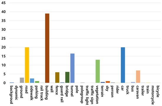
Figure 14.
Class distribution diagram of KITTI-360 dataset.
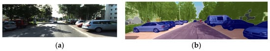
Figure 15.
KITTI-360 Dataset Example: (a) KITTI-360 original image. (b) Segmentation label image.
4.1.2. Cityscapes Dataset
The Cityscapes dataset [25] is a widely used segmentation dataset containing high quality pixel-level annotations of 5000 images (2975, 500, and 1525 for the training, validation, and test sets, respectively) and 20,000 coarsely annotated images collected in street scenes from 50 different cities. Figure 16 shows the number of finely annotated pixels per class of Cityscapes. The original images are 1024 × 2048 in resolution and contain 19 classes in total. We also used the foggy cityscape dataset and rain cityscape to validate our method on high-noise data.
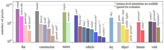
Figure 16.
Number of finely annotated pixels (y-axis) per class (Cityscapes) [25].
Foggy Cityscapes [33] were created by compositing fog onto images of Cityscapes, so they basically have the same structure as Cityscapes. Cityscapes data is organized into 30 classes and eight categories. Classes with small frequencies were excluded, and 19 classes were actually used for compatibility with other benchmark data.
4.2. Specifications of Classic Models
We compared the performance of the proposed model with the well-known UNet, UNet++, UNet3+, Deeplabv1, Deeplabv2, and Deeplabv3 models in semantic segmentation. The models used in this experiment were obtained from reliable online sources. Table 2 lists the information of the models, links to source codes, and backbones of each model used.
Table 2.
Specifications of classical models.
4.3. Comparison of Parameters by Each Model
In this sub-section, the number of learning parameters for each model was compared and analyzed. The number of training parameters for each model was obtained using PyTorch library [34]. Table 3 lists the number of parameters per model.
Table 3.
Number of parameters per model.
Evidently, DeepLabv1 with a single atrous convolution module, used the rate 12 of 3 × 3 kernel, and had the smallest parameter in the DeepLab series, with 20.5 M parameters. DeepLabV2, which includes an ASPP module composed of four atrous convolutions for multi-scale classes, had the most learning parameters of 61 M. DeepLabv3, which inherited the ASPP module, has 58.63 M parameters, almost the same number as DeepLabV2.
UNet++ had more learning parameters compared with the classical U-Net owing to the addition of a dense convolution block to the skip connection. Because UNet3+ reduces the output feature map of the encoder layer to 64 channels and concatenates them, the number of parameters was significantly smaller than those of UNet and UNet++.
In the proposed model, the number of parameters was significantly fewer than those of other models because the decoder layer was generated in a similar way to UNet3+, and the cross-stage method was applied to each layer. These techniques transfer information that is effective for segmentation to other layers, such as the organ boundaries included in low-level feature maps. Therefore, the proposed model had few training parameters but guaranteed higher accuracy. In addition, it had approximately 78% and 36% fewer parameters compared with DeepLapv2, which has the most parameters, and DeepLabv1, respectively.
4.4. Comparison Results by Performance Index
To evaluate the performance of the proposed system, the performance index of Equation (12) and mean intersection over union (mIOU) were used.
where TP is the true positive; FP is the false positive; FN is the false negative; and TN is the true negative.
No post-processing tool was applied for the models and the results of each were optimized using the cross-entropy loss function. Table 4 lists the performance metrics for each model. In terms of precision, DeepLabv3 had the best performance of all the models, with a value of 0.850, which was approximately 1% better than the proposed model. The recall performance of the proposed model was the best, at 0.824, and compared with DeepLabv1 and UNet3+, it was superior by 12% and 0.7%, respectively. The F1-score of DeepLabv1 was the lowest, at 0.726. The F1-score of the proposed model was approximately 0.7% and 13.5% higher than that of UNet3+ and DeepLabv1, respectively, and was the best, at 0.824. In terms of the mIoU, which is the most important indicator in the field of semantic segmentation, the proposed model was approximately 0.7% to 17% better than the other models.
Table 4.
Performance metrics for each model.
As can be seen from Table 4, the proposed model was the best based on the three indicators and exhibited superior performance compared with other models. In particular, as discussed in Section 3.2, our model exhibited the best performance with the fewest parameters of all the models.
4.5. Comparison of Performance of Loss Functions
In this study, the performance of the proposed model was evaluated based on the various loss functions described in the previous section. Table 5 presents the performance results of the proposed model for each loss function and combination. Cross-entropy was outperformed by the focal loss function and other combinations, and the combination proposed herein (focal + IoU + MS−SSIM) exhibited the best performance. Therefore, an appropriate combination of loss functions was required for excellent semantic segmentation.
Table 5.
Performance indicators based on loss function.
4.6. Comparison of Performance of Semantic Segmentation
The performance of each model at semantic segmentation is discussed in this subsection. The performance of each model was evaluated using the mIoU of the 12 classes, and the results are listed in Table 6. Table 6 is arranged from left to right, based on the mIoU values among the classes. The first column shows the individual models, and the second to 12th columns show the mIoU of the individual classes. The last column presents the average mIoU for each model. Deeplabv2, Deeplabv3, and the proposed model exhibited the best results for each of the five classes.
Table 6.
Performance metrics for each model.
Evidently, the proposed model exhibited good performance in the low-frequency model, and Deeplabv2 exhibited excellent performance in the high-frequency class in the dataset. In addition, the proposed model exhibited the best performance in terms of the average mIoU for all classes.
Figure 17 shows the visualization results of each model using the KITT-360. In Figure 18, the original images contain simple classes, and all models exhibited stable performance in the visualization results. Figure 18 shows the visualization results with more complex classes than those in Figure 17. As shown in Figure 18, the proposed model was superior to the other models. Numerous false positives were confirmed in the case of DeepLabv3 owing to shadows in images containing several classes.
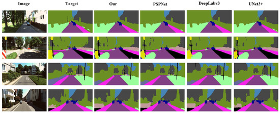
Figure 17.
Visualization results on KITT-360 (including simple class).
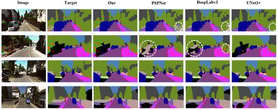
Figure 18.
Visualization results on KITT-360 (including complex class).
4.7. Performance Comparison for Cityscapes Data and High-Noise Data
4.7.1. Cityscapes Data
We evaluated our model with only fine annotated cityscapes data and used 2975 training, 500 validation, and 1525 test images. The results can be found in Table 7. The results in Table 7 indicate that our model has superior performance compared to other models in seven classes. Additionally, the average mIOU of our model across all classes is about 11% better than Deeplabv3. Significantly, the classes with excellent results are those with low frequency, as shown in Figure 16. Therefore, the proposed model has an excellent performance in the field using small training data. Figure 19 shows the results through the dataset of cityscapes. Unlike other models, we show the results of finding detailed features. As an example, extracting features for thin columns shows higher performance than other models.
Table 7.
Performance comparison of each model on the Cityscape dataset.
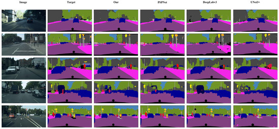
Figure 19.
Visualization results on Cityscapes (including complex class).
4.7.2. Cityscapes Data with High-Noise
In this experiment, we evaluated the model’s performance on noisy data. Foggy and Rain Cityscapes is a dataset that composites fog and rain over natural scenes. The images are rendered using the images and depth maps from Cityscapes [33]. Table 8 and Table 9 show the performance comparison of each model on the Foggy and Rain Cityscape dataset, respectively. In Table 8, we can see that the proposed model performs better than other models in the nine classes.
Table 8.
Performance comparison of each model on the Foggy Cityscape dataset.
Table 9.
Performance comparison of each model on the Rain Cityscape dataset.
This result is an improvement over the previous results from the original Cityscape dataset. Moreover, Table 9 shows the dramatic performance of our model on the more noisy Rain Cityscape dataset. In addition, as shown in Figure 20, the proposed model shows excellent performance for image segmentation in fog and rain situations.
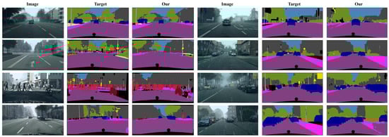
Figure 20.
Visualization results on Cityscapes with rain and fog (including complex class).
5. Discussion
The proposed model had few training parameters by the two-step cross-stage. Reducing the learning parameters of the model can reduce the training time of the model and alleviate the overfitting problem. As shown in Table 3, our model has significantly fewer parameters compared to DeepLabv3 and UNet3+. In Table 6, the mIOU performance of the proposed model and the performance on low-frequency data are not clearly different from other models. However, in Table 7, Table 8 and Table 9, the advantages of the proposed model are evident. Our model has an advantage in the overfitting problem due to small parameters. Therefore, it performs well in low-precision classes. This result is a great advantage in realistic semantic segmentation problems with complex classes.
Our model reduces many learning parameters by applying cross-stage to both the decoder and encoder. However, extreme reduction of the parameters may result in a disadvantage in the accuracy of the model. Therefore, we improved the performance of the proposed model by applying a 4-part ASPP (multi(ML)-ASPP) between the encoder and decoder. The application of ML-ASPP results in an increase in learning parameters, but better transfers details of various features of the input image to the decoder stage. These advantages of our model can be clearly seen in the high-noise dataset experiments and Table 8 and Table 9. In Table 8 and Table 9, we can see that the proposed model performs better than other models in the 9 classes and 12 classes, respectively. These results prove that our model reflects the feature information of the input image better than other models and is robust against noise.
6. Conclusions
A new encoder–decoder-based semantic segmentation model that combines an ML-ASPP and a two-step cross-stage was proposed in this study. The ML-ASPP of the proposed model transferred coarse or contextual information, such as class boundaries in high-resolution features, to the decoder. A two-step cross-stage was applied to the encoder and decoder stages; it reduced the learning parameters of the entire model to enable fast computation. The performance of the proposed model was evaluated and compared with the classical models using the KITTI-360 2D segmentation dataset and Cityscapes. In addition, the number of training parameters of the proposed model was compared with the other models. Further, performance evaluation was performed using various loss functions, and the mIoU results for each class were compared and analyzed. The proposed model had an average mIoU of 0.729 for all the classes, and a performance improvement of approximately 17% compared with DeepLabv1, which exhibited the lowest performance. In Cityscapes data with high noise, we can see that the proposed model performs better than other models in the 9 classes and 12 classes, respectively.
Author Contributions
Conceptualization, methodology and software, M.-H.P.; investigation, J.-H.C.; writing and original draft preparation, Y.-T.K.; All authors have read and agreed to the published version of the manuscript.
Funding
This work was supported by Korea Institute of Planning and Evaluation for Technology in Food, Agriculture and Forestry (IPET) through Open Field Smart Agriculture Technology Short-term Advancement Program, funded by Ministry of Agriculture, Food and Rural Affairs (MAFRA) (122032-03-1SB010).
Data Availability Statement
Not applicable.
Conflicts of Interest
The authors declare that there are no conflict of interest regarding the publication of this article.
References
- Atif, N.; Bhuyan, M.; Ahamed, S. A Review on Semantic Segmentation from a Modern Perspective. In Proceedings of the International Conference on Electrical, Electronics and Computer Engineering (UPCON), Aligarh, India, 8–10 November 2019; pp. 1–6. [Google Scholar]
- Mo, Y.; Wu, Y.; Yang, X.; Liu, F.; Liao, Y. Review the state-of-the-art technologies of semantic segmentation based on deep learning. Neurocomputing 2022, 493, 626–646. [Google Scholar] [CrossRef]
- Long, J.; Shelhamer, E.; Darrell, T. Fully convolutional networks for semantic segmentation. In Proceedings of the IEEE Conference on Computer Vision and Pattern Recognition, Boston, MA, USA, 12 June 2015; pp. 3431–3440. [Google Scholar]
- Badrinarayanan, V.; Kendall, A.; Cipolla, R. Segnet: A deep convolutional encoder-decoder architecture for image segmentation. IEEE Trans. Pattern Anal. Mach. Intell. 2017, 39, 2481–2495. [Google Scholar] [CrossRef] [PubMed]
- Ronneberger, O.; Fischer, P.; Brox, T. U-net: Convolutional Networks for Biomedical Image Segmentation. In Proceedings of the International Conference on Medical Image Computing and Computer-Assisted Intervention, Munich, Germany, 5–9 October 2015; pp. 234–241. [Google Scholar]
- Huang, H.; Lin, L.; Tong, R.; Hu, H.; Zhang, Q.; Iwamoto, Y.; Han, X.; Chen, Y.-W.; Wu, J. Unet 3+: A full-scale connected unet for medical image segmentation. In Proceedings of the IEEE International Conference on Acoustics, Speech and Signal Processing (ICASSP), Barcelona, Spain, 4–8 May 2020; pp. 1055–1059. [Google Scholar]
- Zhou, Z.; Rahman Siddiquee, M.M.; Tajbakhsh, N.; Liang, J. Unet++: A nested u-net architecture for medical image segmentation. In Deep Learning in Medical Image Analysis and Multimodal Learning for Clinical Decision Support; Springer: Berlin/Heidelberg, Germany, 2018; pp. 3–11. [Google Scholar]
- Chen, L.-C.; Papandreou, G.; Kokkinos, I.; Murphy, K.; Yuille, A.L. Semantic image segmentation with deep convolutional nets and fully connected crfs. arXiv 2014, arXiv:1412.7062. [Google Scholar]
- Chen, L.-C.; Papandreou, G.; Kokkinos, I.; Murphy, K.; Yuille, A.L. Deeplab: Semantic image segmentation with deep convolutional nets, atrous convolution, and fully connected crfs. IEEE Trans. Pattern Anal. Mach. Intell. 2017, 40, 834–848. [Google Scholar] [CrossRef] [PubMed]
- Chen, L.-C.; Papandreou, G.; Schroff, F.; Adam, H. Rethinking atrous convolution for semantic image segmentation. arXiv 2017, arXiv:1706.05587. [Google Scholar]
- Lafferty, J.; McCallum, A.; Pereira, F.C. Conditional Random Fields: Probabilistic Models for Segmenting and Labeling Sequence Data. 2001. Available online: https://repository.upenn.edu/cis_papers/159/ (accessed on 2 November 2022).
- Levi, D.; Garnett, N.; Fetaya, E.; Herzlyia, I. StixelNet: A Deep Convolutional Network for Obstacle Detection and Road Segmentation. In Proceedings of the British Machine Vision Conference, Swansea, UK, 7–10 September 2015; p. 4. [Google Scholar]
- Oliveira, G.L.; Burgard, W.; Brox, T. Efficient deep models for monocular road segmentation. In Proceedings of the IEEE/RSJ International Conference on Intelligent Robots and Systems (IROS), Daejeon, Korea, 9–14 October 2016; pp. 4885–4891. [Google Scholar]
- Romera, E.; Alvarez, J.M.; Bergasa, L.M.; Arroyo, R. Erfnet: Efficient residual factorized convnet for real-time semantic segmentation. IEEE Trans. Intell. Transp. Syst. 2017, 19, 263–272. [Google Scholar] [CrossRef]
- Pizzati, F.; García, F. Enhanced free space detection in multiple lanes based on single CNN with scene identification. In Proceedings of the IEEE Intelligent Vehicles Symposium (IV), Paris, France, 9–12 June 2019; pp. 2536–2541. [Google Scholar]
- Scheck, T.; Mallandur, A.; Wiede, C.; Hirtz, G. Where to drive: Free space detection with one fisheye camera. In Proceedings of the Twelfth International Conference on Machine Vision (ICMV 2019), Amsterdam, The Netherlands, 16–18 November 2020; pp. 777–786. [Google Scholar]
- Hou, Y.; Ma, Z.; Liu, C.; Loy, C.C. Learning Lightweight Lane Detection Cnns by Self Attention Distillation. In Proceedings of the IEEE/CVF International Conference on Computer Vision, Seoul, Korea, 27–28 October 2019; pp. 1013–1021. [Google Scholar]
- Paszke, A.; Chaurasia, A.; Kim, S.; Culurciello, E. Enet: A deep neural network architecture for real-time semantic segmentation. arXiv 2016, arXiv:1606.02147. [Google Scholar]
- Chan, Y.-C.; Lin, Y.-C.; Chen, P.-C. Lane Mark and Drivable Area Detection Using a Novel Instance Segmentation Scheme. In Proceedings of the IEEE/SICE International Symposium on System Integration (SII), Paris, France, 14–16 January 2019; pp. 502–506. [Google Scholar]
- Jung, H.G.; Kim, D.S.; Yoon, P.J.; Kim, J. Parking Slot Markings Recognition for Automatic Parking Assist System. In Proceedings of the IEEE Intelligent Vehicles Symposium, Shanghai, China, 13–15 June 2006; pp. 106–113. [Google Scholar]
- Riid, A.; Pihlak, R.; Liinev, R. Identification of Drivable Road Area from Orthophotos Using a Convolutional Neural Network. In Proceedings of the 17th Biennial Baltic Electronics Conference (BEC), Tallinn, Estonia, 6–8 October 2020; pp. 1–5. [Google Scholar]
- He, K.; Zhang, X.; Ren, S.; Sun, J. Deep Residual Learning for Image Recognition. In Proceedings of the IEEE Conference on Computer Vision and Pattern Recognition, Las Vegas, NV, USA, 27–30 June 2016; pp. 770–778. [Google Scholar]
- Qiao, D.; Zulkernine, F. Drivable Area Detection Using Deep Learning Models for Autonomous Driving. In Proceedings of the 2021 IEEE International Conference on Big Data, Orlando, FL, USA, 15–18 December 2021; pp. 5233–5238. [Google Scholar]
- Liao, Y.; Xie, J.; Geiger, A. KITTI-360: A Novel Dataset and Benchmarks for Urban Scene Understanding in 2D and 3D. IEEE Trans. Pattern Anal. Mach. Intell. 2022. [Google Scholar] [CrossRef] [PubMed]
- Cordts, M.; Omran, M.; Ramos, S.; Rehfeld, T.; Enzweiler, M.; Benenson, R.; Franke, U.; Roth, S.; Schiele, B. The Cityscapes Dataset for Semantic Urban Scene Understanding. In Proceedings of the IEEE Conference on Computer Vision and pattern Recognition, Las Vegas, NV, USA, 27–30 June 2016; pp. 3213–3223. [Google Scholar]
- Zhao, H.; Shi, J.; Qi, X.; Wang, X.; Jia, J. Pyramid Scene Parsing Network. In Proceedings of the IEEE Conference on Computer Vision and Pattern Recognition, Honolulu, HI, USA, 21–26 July 2017; pp. 2881–2890. [Google Scholar]
- Huang, G.; Liu, Z.; Van Der Maaten, L.; Weinberger, K.Q. Densely Connected Convolutional Networks. In Proceedings of the IEEE Conference on Computer Vision and Pattern Recognition, Honolulu, HI, USA, 21–26 July 2017; pp. 4700–4708. [Google Scholar]
- Wang, C.-Y.; Liao, H.-Y.M.; Wu, Y.-H.; Chen, P.-Y.; Hsieh, J.-W.; Yeh, I.-H. CSPNet: A New Backbone That Can Enhance Learning Capability of CNN. In Proceedings of the IEEE/CVF Conference on Computer Vision and Pattern Recognition Workshops, Seattle, WA, USA, 14–19 June 2020; pp. 390–391. [Google Scholar]
- Lin, T.-Y.; Goyal, P.; Girshick, R.; He, K.; Dollár, P. Focal loss for dense object detection. In Proceedings of the IEEE International Conference on Computer Vision, Venice, Italy, 22–29 October 2017; pp. 2980–2988. [Google Scholar]
- Máttyus, G.; Luo, W.; Urtasun, R. Deeproadmapper: Extracting Road Topology from Aerial Images. In Proceedings of the IEEE International Conference on Computer Vision, Venice, Italy, 22–29 October 2017; pp. 3438–3446. [Google Scholar]
- Wang, Z.; Simoncelli, E.P.; Bovik, A.C. Multiscale Structural Similarity for Image Quality Assessment. In Proceedings of the The Thirty-Seventh Asilomar Conference on Signals, Systems and Computers, Pacific Grove, CA, USA, 9–12 November 2003; pp. 1398–1402. [Google Scholar]
- Zhou, W. Image quality assessment: From error measurement to structural similarity. IEEE Trans. Image Process. 2004, 13, 600–613. [Google Scholar]
- Sakaridis, C.; Dai, D.; Van Gool, L. Semantic foggy scene understanding with synthetic data. Int. J. Comput. Vis. 2018, 126, 973–992. [Google Scholar] [CrossRef]
- Paszke, A.; Gross, S.; Massa, F.; Lerer, A.; Bradbury, J.; Chanan, G.; Killeen, T.; Lin, Z.; Gimelshein, N.; Antiga, L. Pytorch: An imperative style, high-performance deep learning library. Adv. Neural Inf. Process. Syst. 2019, 32. [Google Scholar]


Disclaimer/Publisher’s Note: The statements, opinions and data contained in all publications are solely those of the individual author(s) and contributor(s) and not of MDPI and/or the editor(s). MDPI and/or the editor(s) disclaim responsibility for any injury to people or property resulting from any ideas, methods, instructions or products referred to in the content. |
© 2023 by the authors. Licensee MDPI, Basel, Switzerland. This article is an open access article distributed under the terms and conditions of the Creative Commons Attribution (CC BY) license (https://creativecommons.org/licenses/by/4.0/).