Abstract
The PLM concept implies the use of heterogeneous information resources at different stages of the product life cycle, the joint work of which allows the user to effectively solve the problems of product quality and various costs. According to the principle of isomorphism of complex systems’ regularities, an effective PLM system must have these regularities. Unfortunately, this principle is not often fundamental when designing PLM systems. The purpose of this paper is to develop principles, based on the general theory of systems, for the design, operation and use of PLM systems and the implementation on their basis of the educational framework of a PLM system for threaded connections with the possibility of its effective development, research and study. The multi-agent approach to the development of a PLM system provides the necessary prerequisites for the emergence of system-wide regularities in it. The parallel work of agents is implemented using the actor model and the Ray Python-package. Agents for the logical inference of knowledge base facts, CAD/FEA/CAM/SCADA agents, agents for optimization by various methods, and other agents have been developed. Open-source software was used to develop the system. Each agent has relatively simple behavior, implemented by its rule function, and can interact with other agents. The system can work in interactive mode with the user or in automatic mode according to a simple algorithm: the rule functions of all agents are executed until at least one of them returns a value other than None. Examples of the system operation are given and system-wide regularities such as emergence, historicity and self-organization are demonstrated in it.
1. Introduction
The product life cycle consists of the stages of design preparation, technological preparation of production, production and operation. At each stage of life cycle, appropriate approaches, methods, tools, knowledge and other information resources are used that help improve the quality of the product. The PLM (Product Lifecycle Management) [1,2,3] concept provides for combining these resources into a system to achieve a super-additive (synergy, emergence) effect [4]. Recent PLM solutions such as Siemens PLM Software (UGS), Dassault system software, Oracle/AgileSoft, PTC/Windchill, SAP/mySAP PLM integrate functions such as Project/Portfolio, CAD/CAM, Product Data Management, Manufacturing Process Management, various types of collaboration, etc. [3]. A PLM system is an information system of heterogeneous information resources, the purpose of which is to provide information support for the stages of the life cycle of a product in order to improve the quality and reduce costs.
How to effectively combine these resources into a system? The answer must be sought by analyzing other complex systems. The most important principle of systems theory is the principle of isomorphism of regularities of systems [5]. According to this principle, a PLM system, as a complex system, must have regularities of complex systems such as emergence, integrativity, “requisite variety”, hierarchy, historicity, non-linearity, self-organization, two-phase evolution, adaptation, feedbacks (negative and positive or “damping” and “amplification”), self-similarity, openness, additivity and progressive factorization, memory, and must also have a structure similar to them [4]. Unfortunately, when developing PLM systems, this important principle is not often paid attention to [3,4]. Partially, these regularities are used in systems engineering [6] and systems analysis [7] techniques. In particular, the regularities of emergence, historicity, “requisite variety” and spontaneous order are noticeable in the systems analysis method of “gradual formalization of the decision-making model” [7]. The authors of the method note that most of projects of complex systems need to be described by a class of self-organizing systems; the models of which must be constantly adjusted and developed. The product life cycle should be isomorphic to the life cycle of other complex systems. The paper [4] shows its correspondence to the activity cycle. Methodologists point out the importance of studying the phenomenon of activity: “activity is the only thing that exists from the very beginning, and nature is a certain construction of activity itself” [8]. Figure 1 shows the main stages of activities related to PLM [4].
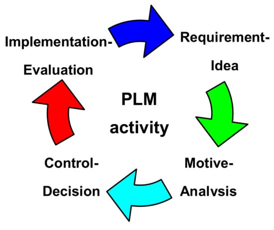
Figure 1.
Stages of PLM activity.
At the Requirement-Idea stage, the requirements for the product and the idea of quality improvement are formulated, the resources of conceptual design, conceptual modeling (CAID—Computer Aided Industrial Design), heuristic methods, methods of activating the intuition of specialists (MAIS) [4,7] are used. The Motive-Analysis stage analyzes these requirements and ideas, typically using methods of formalized representation of systems (MFRS) [4,7], and indicates how these requirements and ideas can be implemented. At the Control-Decision stage, final decisions are made and the product is produced. At the Implementation-Evaluation stage, the product is operated with an assessment of its quality relative to its preliminary version. As a result of these assessments, new requirements and ideas for improving the product may arise. That is, several consecutive cycles actually form a helix, where all the turns are similar in structure, but correspond to different levels of product quality—with each turn of the helix, the quality improves and new requirements and ideas are implemented [4]. According to the regularities of hierarchy and fractality [5], each stage can be similar in structure to one turn and consist of sub-stages similar to the listed stages, which are also isomorphic to the life cycle, etc. For example, a technological preparation stage could have Requirement-Idea, Motive-Analysis, Control-Decision, Implementation-Evaluation sub-steps, but related to the technological process [9].
Complex systems such as biological, social or economic systems have life cycles that are driven by evolution and consist of a large number of heterogeneous, decentralized, autonomous and relatively simple elements. A multi-agent approach [10,11,12,13,14] can provide such a structure of an information system and create the prerequisites for the emergence of system-wide patterns in it.
Many implementations of multi-agent PLM, among which the ontology-based approach is often used, testify to their effectiveness. These approaches provide a high level of integrativity. In particular, a new approach, based on the ontology, the Semantic Web and the concept of agent, was proposed in [15]. In [16], the multi-agent system integrates the problem-solving method 8D, Process Failure Mode and Effect Analysis, Case-Based Reasoning, and PLM. The architecture of the system is based on SEASALT [17] (Shared Experience using an Agent-based System Architecture LayouT), which is a multi-case base domain-independent reasoning architecture for extracting, analyzing, sharing, and providing experiences. In [18,19], the agent technology is used in the solution to support decision-making in the design of recycling-oriented products. In [20], a knowledge engineering multi-agent module integrated in a PLM system which is based on a multi-domain scheme (project, product, process and use) taking into consideration several viewpoints (structural, functional, dynamic, etc.) was shown. In [21], a generic multi-agent framework using IoT-based protocol, as the communication medium, for PLM of the products having high collateral damage values and where monitoring and control of systems in real-time are vital, was developed. In [22], a multi-agent software architecture that allows the capitalization of distributed and heterogeneous knowledge was designed. The research of [23], targets the development of a knowledge engineering multi-agent system integrated into a PLM environment linked with virtual reality tools. In [24], a PLM framework supported by a proactive approach based on intelligent agents was proposed. The paper [25] describes the process and various details of developing the semantic object model into an ontology using OWL-DL. The purpose of this study [26] is to create, analyze. And reuse an ontology-based approach during the implementation of a multi-agent system that is capable of integrating different elements of a distributed control system. In [27], a multi-agent software system for solving and automating tasks related to PLM and a logistics support analysis, was presented.
The holonic paradigm is a major paradigm of intelligent manufacturing systems [28,29]. Such holonic properties, such as a recursive structure, adaptability, autonomy, cooperation, openness, and emergence [29], fully correspond to some system-wide regularities (primarily integrity and hierarchy). Industry 4.0 manufacturing systems key enablers and corresponding holonic properties are analyzed in [29]. Holonic Control Architectures (HCA) may answer to many requirements of the Industry 4.0 [29]. Despite this, HCA researchers rarely mention the fundamental research in systems theory, and they do not start with the principle of isomorphism as the main one. As a result, properties such as historicity and self-organization remain little explored.
The analysis (Table 1) shows that the principle of isomorphism is rarely fundamental in the construction of such systems. Researchers (including HCA researchers) use the “trial and error” method, which, together with ignoring many system-wide patterns, leads to the appearance of fundamental flaws at a certain stage of system development that cannot be eliminated without a radical restructuring of the system.

Table 1.
Some research in PLM using multi-agent and ontological approaches.
The analyzed works usually provide theoretical solutions that are difficult to verify due to the lack of system implementations or their insufficient explanation and documentation. This complicates their verification, research, and development.
Despite the fact that threaded connections seem to be simple products, there is a lot of scientific work related to the problems that appear at different stages of their life cycle, in particular during the design, manufacture, and operation stages [32,33,34].
Specifically important for threaded connections of oil and gas equipment are areas of research such as analytical modeling [35,36,37], investigation of manufacturing errors [38,39,40,41], and corrosion fatigue [42,43,44]. These works contain certain knowledge and methods that, when applying PLM, must be formalized and algorithmized. Due to this and due to the prevalence of such products, we chose an educational PLM system for threaded connection for our research. In [31], using a systematic approach and the Python language, a PLM system for threaded connections was developed. However, only design components have been developed and methods for their asynchronous operation have not been proposed.
The purpose of this paper is to develop principles, based on the general theory of systems, for the design, operation, and use of PLM systems and for their implementation on the basis of the educational framework of a PLM system for threaded connections with the possibility of its effective development, research, and study. To achieve the goal, it is necessary to solve the following tasks:
1. Based on the principles of systems theory, substantiate the basic properties of elements, the architecture of the system, its methods, and tools.
2. Develop basic components covering all stages of PLM activity, with the possibility of their asynchronous operation and further development: knowledge base facts, inference rules, inference engine, CAD, FEA, CAM, and SCADA components, and components for optimization.
3. Show a simple example of using a PLM system for information support of the life cycle of a special threaded connection.
4. Analyze the appearance of regularities of complex systems in the developed PLM system.
2. Methods and Software Tools
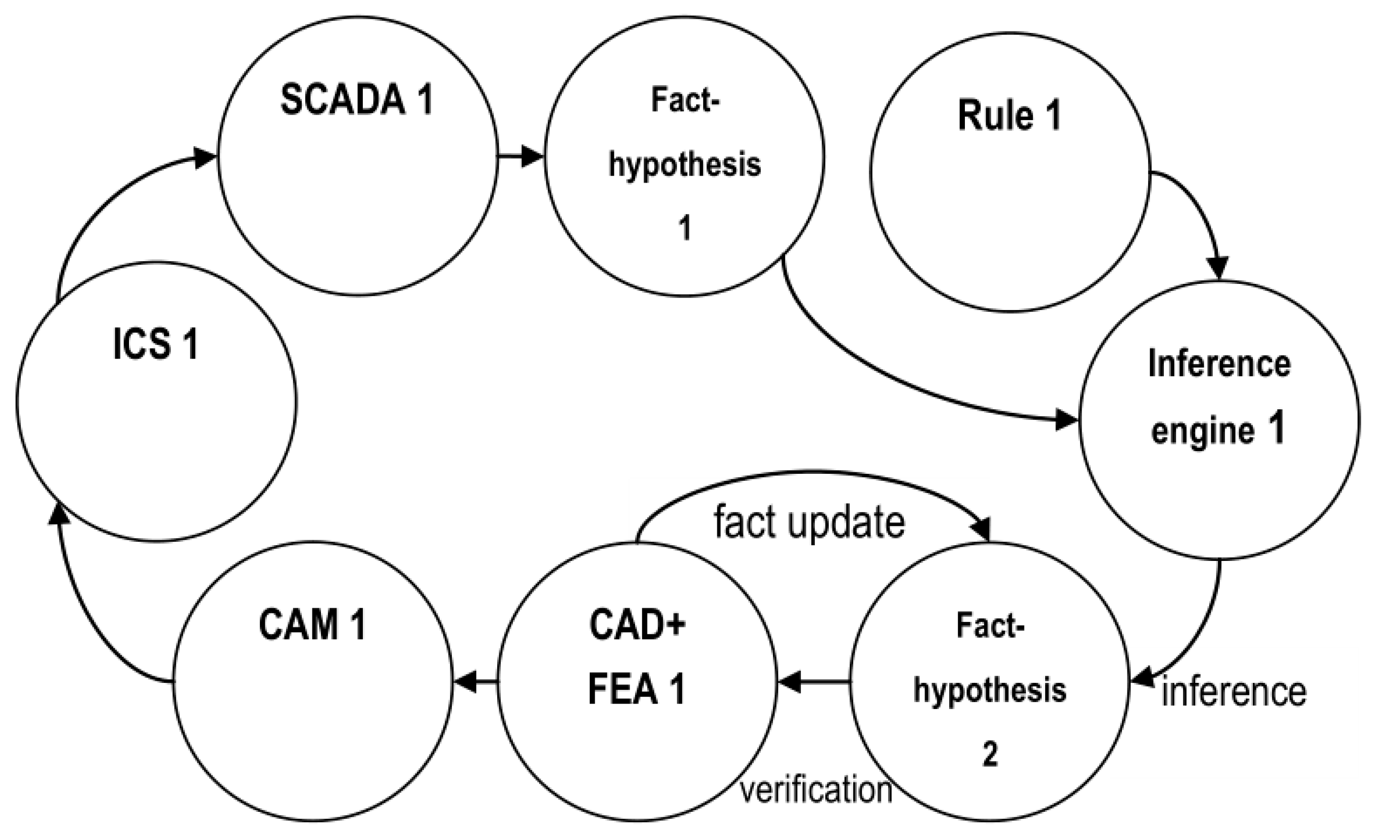
A simple example of a multi-agent PLM system is shown in Figure 2. Agents can implement knowledge base facts (facts, product requirements, and hypotheses for its improvement), inference rules, inference engine, CAD, FEA, CAM, and SCADA components, etc. Hypotheses and rules can be passed to the inference engine for analysis or to obtain new hypotheses, and they are then passed to the “CAD + FEA1” agent for verification by a finite element analysis (FEA) of the performability of the product model. If the analysis results confirm the hypothesis, the data are transferred to the “CAM1” agent to prepare the technological process for the product manufacturing. Otherwise, the hypothesis is not confirmed, and so the relevant facts are updated. Agent “ICS1” (Industrial Control System) manages the manufacturing process. The finished product is subjected to testing or operation, during which the “SCADA1” (Supervisory Control and Data Acquisition) agent monitors the technical condition of the product. Based on the results from monitoring, new requirements and hypotheses may appear, initiating a new turn of the helix. At any stage of the life cycle, it should be possible to interrupt the cycle and return to the previous stages.

Figure 2.
An example of a multi-agent PLM system.
The paper [30] reviews many methodologies for creating multi-agent systems. However, it does not discuss the need to introduce a transdisciplinary meta-methodology that uses the principle of isomorphism and allows a functional synthesis of methodologies, the effectiveness of which has been proven by the long evolution of other systems. In particular, the elements must have properties that create the prerequisites for the appearance in the system of patterns of complex systems. An analysis of many systems shows that, first of all, the main properties are openness, autonomy, and adaptability. These properties imply an ease of creation and modification of the PLM system’s elements, their asynchronous operation, and their flexibility of knowledge representation. In this regard, the authors propose to use the Python [45] general-purpose programming language, which is known for its simplicity and flexibility, combined with the Ray package to develop the elements.
Due to the need to ensure adaptability, the authors recommend, first of all, using free software, which is associated with the following advantages: the open-source nature, potentially unlimited developer community, intensive development, collaborative development opportunities, user independence from manufacturers, and high degree of interoperability and scalability [46]. In particular, the user can use the CalculiX [47] finite element analysis system, the Gmsh [48] finite element mesh generator, the OpenModelica [49] dynamic systems simulation environment, and the GRBL [50] CNC machine control software. However, to expand the capabilities of the system, it should also be possible to use commercial programs available via the API. These could be any of the following: SOLIDWORKS, 3D CAD/CAE/CAM-system; Abaqus/CAE, finite element analysis system with Python API; fe-safe, fatigue life analysis system; or other software. Ideally, the system architecture should allow agents to be programmed in any language and not depend on the platform, for example, as service-oriented software architecture allows. The user should also pay attention to indicators of software quality such as usability, maintainability, and performance. Due to the fact that the components should be heterogeneous, decentralized, autonomous, and relatively simple, their development should adhere to the well-known concept from the Unix philosophy “Do One Thing And Do It Well”. This concept is related to the regularity of the specialization of elements and their “requisite variety”. To develop the components of the PLM educational system and their system integration, the authors used the popular Python language, for which many different packages have been developed. For the PLM system, the following Python packages can be used: pythonocc [51], Python wrapper for the Open CASCADE Technology [52] geometry kernel; FreeCAD [53], 3D CAD; NumPy [54], package for N-dimensional arrays; SciPy [55], basic library for scientific computing; Matploltlib [56], creating 2D diagrams; Sympy [57],symbolic mathematics; scikit-learn [58], machine learning; Pycalculix [59], FEA based on CalculiX and Gmsh; and Jupyter [60], interactive computing.
The following software versions were used in this paper: Python 3.8.9x64, NumPy 1.22.4+mkl, SciPy 1.7.3, Matplotlib 3.5.0, Ray 1.8.0, Pycalculix 1.1.4, Pyserial 3.5, Jupyter Notebook 6.4.6, SymPy 1.10.1, Gmsh-4.8.4-Windows64, and CalculiX 2.16.
An important performance issue of the PLM system is to ensure the parallel operation of agents. Ordinary synchronous functions are executed sequentially—before calling the function again, the user should wait for the result of the previous call. An asynchronous function can be called without such a wait [61]:
  @ray.remote
  def f():
      return 1

  obj_ref1 = f.remote() # asynchronous call
  obj_ref2 = f.remote() # one more
  ray.get(obj_ref1) # result
  ray.get(obj_ref2)
To implement parallelism and asynchronous calls, the actor model and the Ray Python package were used. Ray is an open-source package that makes it easy to scale any computationally intensive Python program [61]. The Ray Core package provides simple primitives for creating parallel and distributed Python programs with minimal code changes—the user can easily convert synchronous code to asynchronous by adding the @ray.remote decorator [61]. With Ray, the code will run on a single machine, and it can easily be scaled up to a large cluster [61]. For the FEA example, the simulation can be lengthy and can block the operation of a synchronous system [31]. However, Ray allows the user to create an FEA actor class, an instance of an actor, and run it asynchronously with other actors:
  @ray.remote
  class FEA(object): # actor class
      def rule(self, x=0.1): # function describes the agent’s behavior
          import mypycalculix # import of module implementing FEA
          mypycalculix.hh=x # changing the model parameter value
          return mypycalculix.run() # run simulation and return results

  fea1=FEA.remote() # actor instance
  ro=fea1.rule.remote(0.1) # asynchronous call
  ... # other asynchronous calls
  y=ray.get(ro) # get result
This class for finite element simulation uses the mypycalculix module, which is described below.
For the effective design of threaded connections, it is important to choose a method for constructing various types of helical curves and surfaces. The authors propose to construct a parametric helix equation by sequential transformations of a point object in the space [62]. For example, a point object is described by a position vector
and there is a rotation path transformation around the z-axis
where is the arbitrary function. Then, the position vector describes a circle in the xy plane. The x and y scaling transformation looks like this,
and the z translation transformation like this,
Here, and are the arbitrary functions. Then, the parametric equation of the helix can be obtained using the following transformations:
If the P vector describes not a point, but a curve, then by such transformations one can also obtain the equation of helical surfaces [62].
3. Results
Let us consider an example of an educational PLM system for the threaded connection of plastic parts (polypropylene) with special threads (Figure 3). Many studies show an increase in the strength and tightness of the connection when using special optimized thread profiles. For educational purposes, it is best to use the method of milling for such threads, which also has the following advantages: high cutting speed, productivity [41], flexibility, single-pass processing, and short chips. This product is used for educational purposes only and was chosen due to the ability of the design to optimize parameters and the ability to cut threads with a conventional disc milling cutter on a CNC 3018 Pro 3-axis training milling machine.
Figure 3.
Threaded connection with special thread.
The source code of the developed PLM system is available on GitHub [63]. Each agent of the system is a Ray-actor and has a rule() function that describes its behavior. This function can take arguments and return results.
The inference engine allows the user to derive new facts from existing ones using inference rules, as is completed in the CLIPS production rule system [64]. Facts are represented as triplets (subject, predicate, and object) and are stored in agents of the Fact class, whose rule() function returns a triple. For example, the fact “An equivalent stress of 14 MPa occurs in a structure with a dimension h = 0.1 mm” can be represented as a triple (“Seqv=14”, “match”, “h=0.1”). The inference rules “if A, then B” can be written as follows: A → B, where A, B are facts. For example, the inference rule (X, Y, Z) → (Z, Y, X) should be read as “If there is a fact (X, Y, Z), then infer a new fact (Z, Y, X)”, and the rule (X, Y, Z) and (Z, Y, W) → (X, Y, W)—“If there is a fact (X, Y, Z) and a fact (Z, Y, W), then infer a new fact (X, Y, W)”. Inference rule agents are created using actor classes (Rule1, Rule2), whose rule() functions search for facts corresponding to facts A of the rule and they return the set of inferred facts B. The Reasoner actor class describes the concept of an inference engine. Its rule() function runs (in parallel and once) the rules of the inference rule agents, which are passed triplets with facts, and then it returns a set of triplets with new facts.
The FEA actor class agent simulates the stress–strain state of the connection using an axisymmetric finite element model. The rule() function takes the value of the connection parameter and returns the maximum stress. It uses the mypycalculix.py [63] automated FEA module of a threaded connection, which is developed by the authors and uses Pycalculix [59]. A feature of the Pycalculix package is the ability to easily create parametric models with the ability to automate all stages of model building and create FEA programs for fully automatic parametric studies and design optimization. Before using Pycalculix, the user must specify the path to the CalculiX solver (ccx.exe) and the Gmsh generator (gmsh.exe), the executable files in the file system. The package has the ability to visualize the geometry, mesh, and results using Matplotlib. The disadvantage of the package is its ability to create only two-dimensional models (planar or axisymmetric).
The mypycalculix.py module builds a geometric model of a threaded connection with the given parameters, and it meshes with Gmsh, generates an input solver file, runs a simulation with the CalculiX solver, and gets the results. The description of a parametric model contains all model parameters with their values. The parametric model is created using the Python code in an object-oriented way. In particular, the objects of the geometric model of the part (lines and arcs) are created using the Pycalculix functions, which are passed the values of the model parameters:
  part.goto(r0, 0) # go to the point
  l0=part.draw_line_ax(l) # create a longitudinal line
  l1=part.draw_line_rad(t1) # create a transverse line
where r0, l, and t1 are model parameters.
It is also possible to import a complex geometric model in a DXF format. To facilitate the creation of parametric models, the findLine() function developed by the authors can be used, which searches for the edges of a geometric model by their various attributes: midpoint coordinates, extreme point coordinates, length, etc. In general, the description of the model is similar to the description of models in other FEA packages: geometry creation, description of the mechanical characteristics of materials, description of surface contact, description of the finite element mesh, boundary conditions, and loads. To improve the accuracy of calculations, the size of the mesh elements should be reduced in areas with fine geometry, and especially in areas with a possible stress concentration (Figure 4a). The instructions for building models, calculating, and getting results are located in the run function, and the model parameters are the global variables. In the case of a parametric study (investigation of the influence of a parameter on stress or strain), the run() function should be called for various values of the model parameter, saving the results in a list. For example:
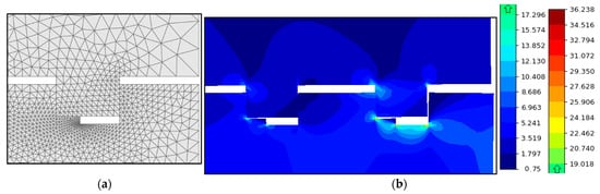
Figure 4.
Finite element mesh (a) and distribution of equivalent stresses (b) in the zone of the first thread turns (MPa).
  X=[8, 10, 12, 14, 16, 18, 20, 22, 24, 26, 28]
  Y=[] # result list
  for x in X: # for each value
      l_=x # change the value of the parameter (l_ is a global variable)
      Y.append(run()) # add result to list
Using the FEA actor, the user can perform these tasks in parallel, which, in the case of a multiprocessor system, will reduce the computation time:
  F=[FEA.remote() for x in X] # create actors
  Y=ray.get([f.rule.remote(x) for x, f in zip(X, F) ]) # execute asynchronously
After receiving the results (stresses or strains), the program can read their values at any node of the mesh or obtain the maximum values. The simulation results (Figure 4b) correspond to the expected ones—in joints of this type, the greatest stresses occur in the zone of the first turns. Thus, according to the results of the analysis, some elements should be provided in the design that would reduce these stresses.
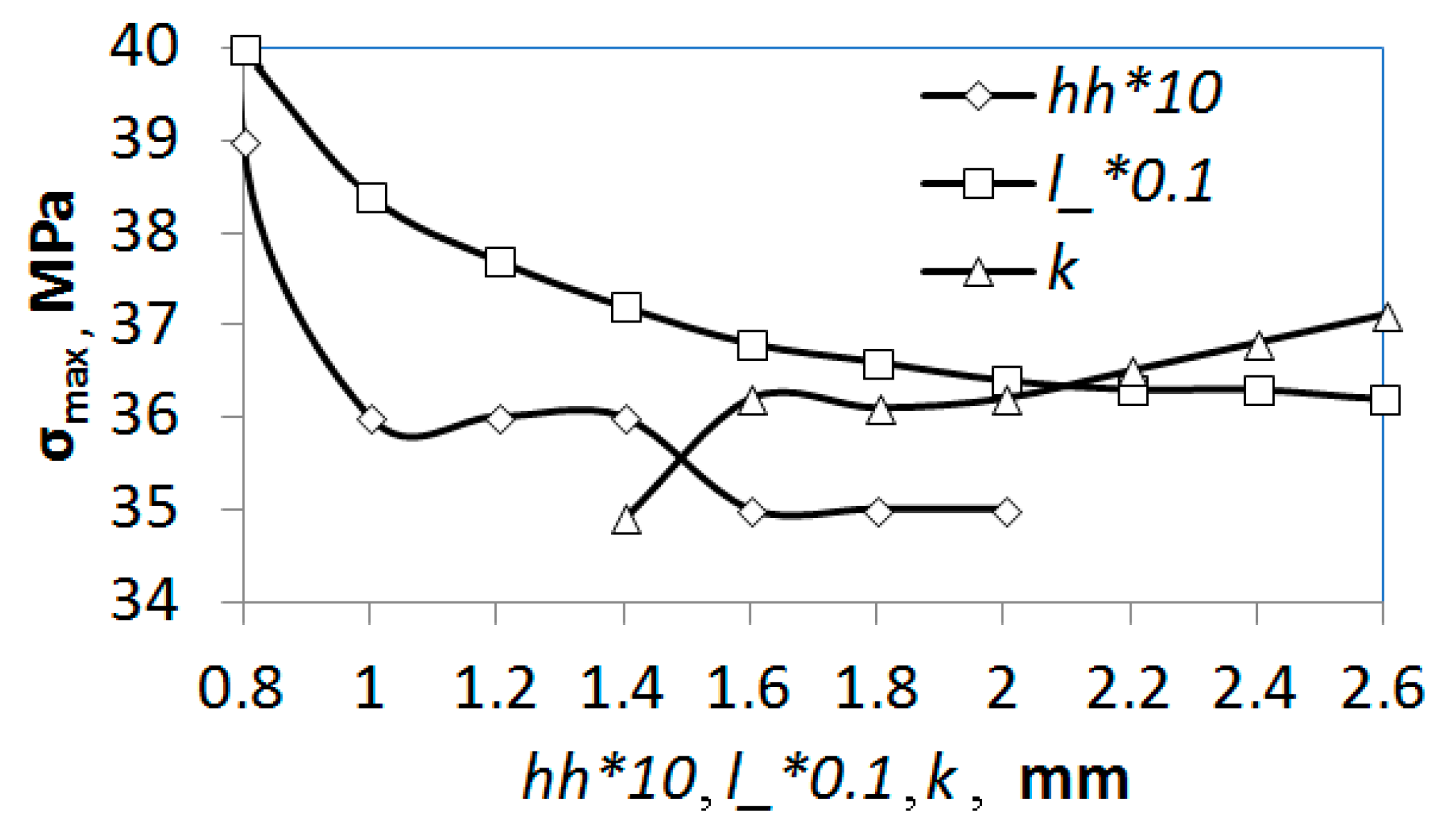
To demonstrate the operation of the module, the dependences of the maximum equivalent stresses in a threaded connection on parameters such as thread length, pitch, and clearance were obtained (Figure 5). However, the maximum stress in a joint is not always a criterion for its durability, so it is necessary to find the stress value in the most dangerous zones where fatigue cracks may appear, for example, in the zone of the first thread root. In many cases, such dependencies can be easily formalized, included automatically [31], and the knowledge base facts can be obtained. For example, from the dependence σmax(l_) (Figure 5), one can observe the fact that: “an increase in the length of the thread leads to a decrease in the maximum stresses”.
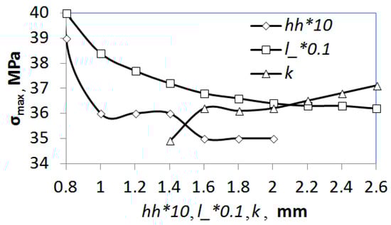
Figure 5.
Dependences of the maximum equivalent stresses σmax in the connection on radial clearance in the thread (hh), thread length (l_), and pitch (k).
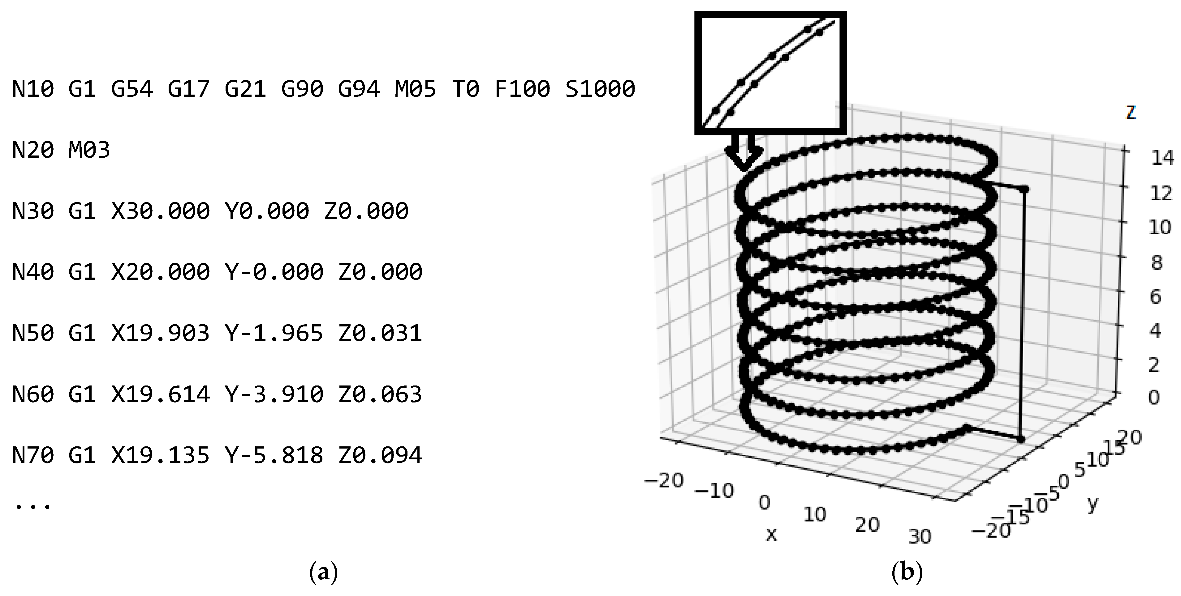
The CAM [63] actor class agent uses the CNC_thread_mill.py [63] module developed by the authors to generate the G-code for thread milling on a three-axis CNC milling machine (Figure 6a). The rule() function takes the value of the connection parameter and returns the corresponding list of G-code points (Figure 6b). The milling of taper external and internal threads with multiple passes and an arbitrary thread profile specified by the point coordinates in the X-Z plane is supported.
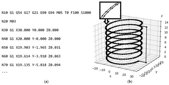
Figure 6.
G-code snippet (a) and toolpath visualization with Matplotlib (b).
The helix Points() function returns a list of helix points [63]. Its parameters are r—minimum radius; h—height; p—pitch; fi—taper angle; n—number of points on one turn; and z0—axial displacement. The coordinates of the points are determined by the parametric helix equation.
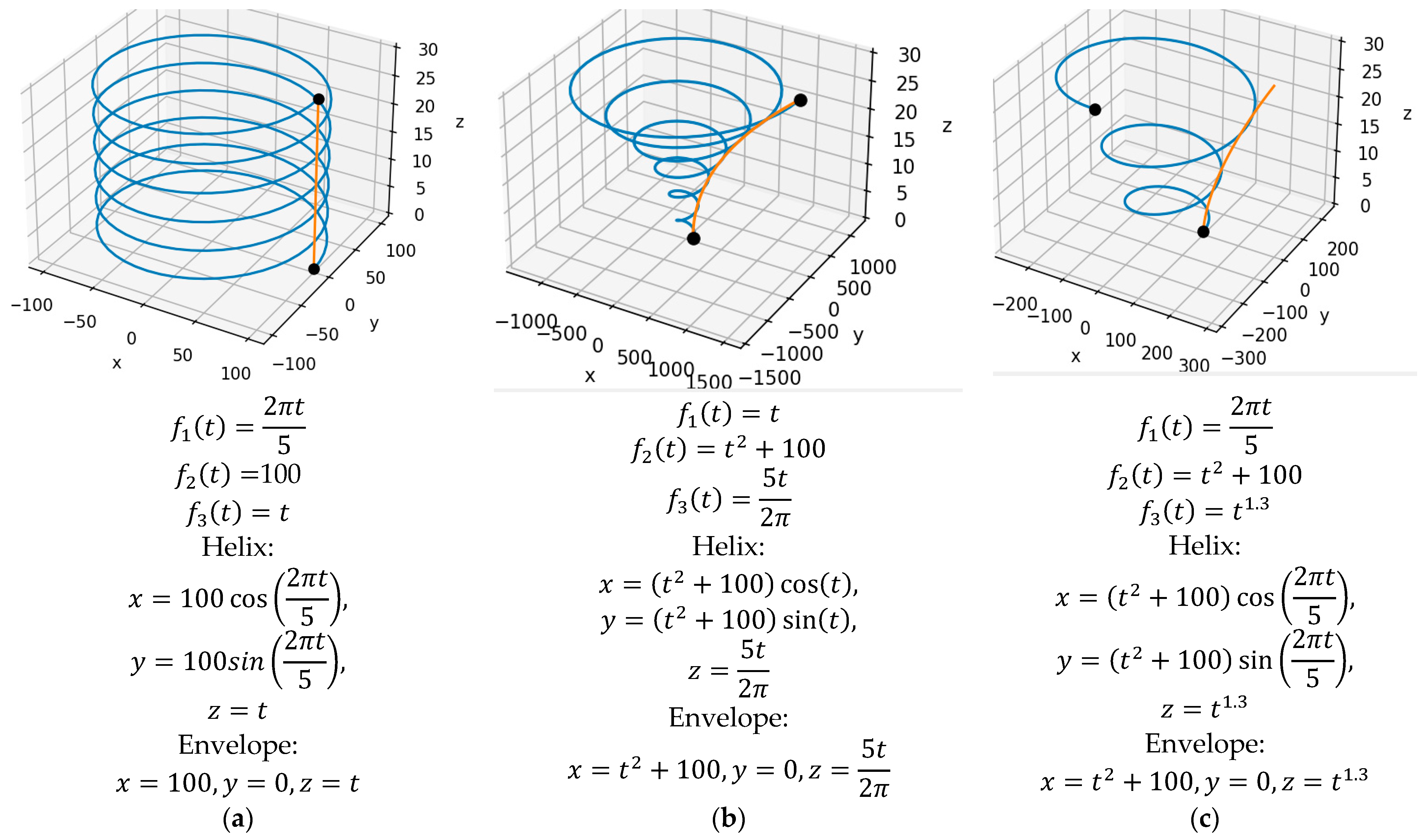
The helixPoints2() function has also been developed, which also returns helix points, but allows the user to build more complex and varied helixes. The function uses the SymPy symbolic mathematics package and the transformations (1). However, the user can easily modify its code to apply additional transformations. If the user defines different functions , , and , this allows different helixes to be obtained. Some of these helixes are shown in Figure 7. Along with helixes, their planar envelope curves obtained using SymPy are shown. Figure 7a shows a cylindrical helix with a radius of 100 and a pitch of 5; in Figure 7b the helix has a parabolic envelope, an initial radius of 100 and a pitch of 5; in Figure 7c the helix is different in that it has a variable pitch.
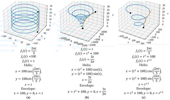
Figure 7.
Helixes (blue color) and their planar envelope curves (red color): cylindrical (a); parabolic (b); parabolic with variable pitch (c).
The parameters of the helixPoints2() function are the strings f1, f2, and f3, which define the functions , , , the helix height h, and the number of points on the helix num. By solving the equation z(t) = h, the algorithm determines the maximum value of the t parameter and generates a list of points. Following is an example of using this function:
  import numpy as np
  from sympy import *
  P=helixPoints2(f1=“2*pi*t/5”, f2=“t**2+100”, f3=“t**1.3”, h=30,
                  num=100, plot=True)
Functions can even be piecewise-defined, which greatly increases the set of different types of curves that can be built. For example, the function
allows the user to create a helix with different pitches—the second part of the curve will have twice the pitch of the first. Then, the f3 parameter in the Python code should be like this “Piecewise((t, t <= 10), (2*t-10, t > 10))”.
The function can be used at the design stage of a threaded connection to create different types of thread helixes. The user can build a morphological matrix in which there are various combinations of , , and , and then select the most promising options or transfer all elements of the matrix to CAD/FEA agents to identify the best options according to stress and strain criteria. Thus, the developed function complies with the principle of «requisite variety» in the threaded connection design subsystem.
The TreadMulti() function uses helixPoints() and returns a list of points for thread milling in multiple passes. Its parameters are h—thread length (should be a multiple of pitch p); p—pitch; fi—taper angle; n—number of points on one turn; and R, Z—lists with radii (x-coordinate) and z-coordinate of the first points helical lines. In other words, R and Z contain the x- and z-coordinates of the profile points. For one pass R=[r], Z=[0], where r is the minimum thread radius.
The Gcode() function returns a G-code from a list of points. The plotCNC() function plots points using Matplotlib. Below is an example of the code generation for thread milling in two passes (Figure 6):
  rf=10 # radius of milling cutter
  # list of points:
  P=TreadMulti(R=[9.5+rf, 9.6+rf], Z=[0, 0.3], h=14, p=2, fi=0, n=64)
  code=Gcode(P, “cnc.txt”) # generate G-code and save to file
The module supports threading on CNC systems that do not have tool radius compensation and circular interpolation. Using Python Streaming Scripts [65], the G-code is transmitted via a serial port to the GRBL program that controls the machine. There is the possibility of organizing a flexible manufacturing system that combines a CNC-machine with an industrial robot designed to install and remove a workpiece. A CNC 3018 Pro educational machine equipped with a control board supporting GRBL software was used. An Arduino Uno can be used as such a board. The workpiece 1 (Figure 8) is installed on the machine table 3 on the cylindrical pin 4, and is fixed with a bolt 2, a washer 5, and a nut 6. The thread is cut with a disc milling cutter 7 in several passes. The user can apply the free application Candle [66] to set up the machine.
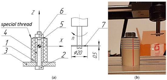
Figure 8.
Technological sketch (a) and photograph (b) of milling a special thread on a CNC 3018 Pro machine.
A SCADA actor class agent is also proposed for monitoring the technical condition of a threaded connection at the testing or operation stage. Its rule function receives the value of the connection parameter and returns the dependence of the deformations on the running time. The agent uses a schema based on an example from Proteus CAD «Arduino HX711 SparkFun Breakout Board with 200 kg Load Cell» [67]. Strain monitoring is performed using an Arduino UNO board, an HX711 chip (24-bit ADC with strain gauge amplifier), and a strain gauge that is glued to the threaded connection. The Arduino sketch sends the results via a serial port using a pyserial package (Table 2) to the HX711proteus_client.py module, which is developed by the authors and associated with the agent. The results can be analyzed and compared with the previous ones and new facts can be obtained.
Table 2.
Programs for data transfer via serial port.
To demonstrate an example of using the PLM system, the authors developed an interactive document: Jupyter notebook [63]. The document contains cells with Python code, cells with formatted text generated by the Markdown markup language, and execution results in the form of text and charts. Ray is initialized first. In this example, the resources of one computer are used for the calculations, but a cluster can also be used. Next, the actor classes described above (Fact, Rule1, Rule2, Reasoner, FEA, CAM, SCADA) and their actor objects (agents) that can work asynchronously are created.
  f1=Fact.remote(“Seqv=14”, “match”, “h=0.1”)
  f2=Fact.remote(“h=0.1”, “match “, “utot=869e-6”)
  f3=Fact.remote(“h=0.2”, “match”, “Seqv=16”)
  r1=Rule1.remote(“match”)
  r2=Rule2.remote(“match”)
  r=Reasoner.remote()
  fea1=FEA.remote()
  cam1=CAM.remote()
  scada1=SCADA.remote()
In this case, the facts f1, f2, and f3 are represented, containing the correspondence between the values of the input and output parameters of the threaded connection model: the geometric parameter h (mm), the maximum equivalent stress in the thread Seqv (MPa), and the maximum total displacement utot (mm). These facts can be obtained as a result of modeling, experiments, and industrial data at the preliminary stages of the life cycle. The inference rules r1 and r2 are for the “match” property, which is symmetric, i.e., (1, match, 3) → (3, match, 1), and transitive, i.e., (1, match, 3) and (3, match, 4) → (1, match, 4).
Each agent works autonomously, receiving the input and returning the results. The agent may return None, which means that there are no new results. The automatic operation of the system can be organized using a simple algorithm: while there are changes in the system, call the rule() function of each agent. If all the agents return None, then automatic operation of the PLM system is terminated. For example, a logical inference is implemented using a naive forward chaining algorithm, namely, call the Reasoner agent’s rule() function while new facts are inferred.
  fs=[f1, f2, f3]
  rs=[r1, r2]
  T=set()
  re=1
  while re:
      re=0
      ts=ray.get(r.triplets.remote(fs))
      tn=ray.get(r.rule.remote(rs, ts))
      if tn:
          T.update(tn)
          re+=1
  print(T)
As a result, the set of knowledge base facts is supplemented by the following:
{('Seqv=16', 'match', 'h=0.2'), ('Seqv=14', 'match', 'utot=869e-6'),
('h=0.1', 'match', 'Seqv=14'), ('utot=869e-6', 'match', 'h=0.1')}
Further in the document, a threaded connection variant is simulated using the FEA agent. Using the fea1 agent, a threaded connection with the h=0.1 mm parameter (gap in the thread) is simulated. We wait for the results.
y1=ray.get(fea1.rule.remote(0.1))
However, all agents have the ability to run the simulation asynchronously, i.e., ro=fea1.rule.remote(0.1), and obtain the result in the cells below, i.e., y1=ray.get(ro).
The calculated maximum values of equivalent stresses and the distribution of strains and stresses in the thread are displayed (Figure 4). G-code generation for milling an external thread variant (h = 0.1) is performed using the CAM agent.
  y2=ray.get(cam1.rule.remote(0.1)) # trajectory points
  import CNC_thread_mill
  CNC_thread_mill.plotCNC(y2) # point visualization
The coordinates of the first points of the generated trajectory and the plot of the trajectory are displayed using Matplotlib (Figure 6b). With the help of a SCADA agent, the technical condition of a threaded connection variant (h = 0.1) is monitored during the operation.
scada1ref=scada1.rule.remote(0.1)
The following commands should be run when scada1.rule() has been completed. A graph of the dependence of deformations on the operating time is displayed.
  X,Y=ray.get(scada1ref)
  import matplotlib.pyplot as plt
  plt.plot(X,Y)
  plt.show()
At any stage of the life cycle, the user can access the desired cells, edit the code, and obtain the results. The user can enter new data, change the model or parameter value, create new agents, and restart the system. Accordingly, at each iteration step, new knowledge appears, and the system evolves, like the product itself. Thus, the multi-agent system works interactively with user interaction.
However, agents for optimization calculations have also been developed that can work autonomously. The Opti base class of agents for optimization has an f attribute, which is the object of optimization and must be a function or ray.actor.ActorHandle. The attribute function calc() calculates the value of f(x) using the FEA agent. The class also contains the attribute function find(), which receives an XY dictionary of arguments and values of the function, and by analyzing these values using a special algorithm, returns the hypothesis of the argument x of the minimum. The attribute function rule() describes the rule of the agent’s behavior in the environment of X and Y values. For all optimization agents, this function has the same implementation with the following general algorithm:
  While XY length is less than 20:
      Get XY from environment
      Find x with find()
      Reserve space in XY environment by key x
      If it's already reserved, go to the next iteration
      Calculate the value of f(x) and write it to the environment by key x
The loop continuation condition is a condition for the continuation of optimization calculations. It may be different. For example, it can be like the following:
where SD is the standard deviation and i is the index of the minimum value in the Y array. In Python, this condition can be written as Y[i-2:i+3].std()>0.01. However, the restriction on the length of XY (len(XY)<20) is better to apply in case of a certain time limit for optimization calculations.
The OptiX class inherits from Opti and is designed to find the minimum using the grid stochastic method. It differs from Opti only in the find() function. In this case, its algorithm is as follows:
  Get indices I for sort Y
  Choose a random index i from I (the probability of choosing
  increases towards the beginning of the list I)
  Given index i find index j of element in Y
  Find index k of neighboring element on the left (k=j-1) or right (k=j+1)
  Find x=(X[i]+X[k])/2
This method is a combined global optimization method that requires an initial grid of x values with a desirably uniform step. At each step, it finds x, which is the same distance from the optimal value (found at the previous iteration) and the neighbors to the right or left (random choice). In order to not become stuck in a local minimum, the algorithm provides a random choice of x according to a given distribution law, the parameters of which can be changed.
The OptiR class inherits from Opti and is designed to find the minimum by building a regression model of the XY data. The F attribute is a function of the model, such as a second- or third-degree polynomial. The fit() function uses the method of least squares to find the best XY data model and returns the value of its coefficients and the coefficient of determination R2. The find() function finds the minimum of this model using a grid method with a sufficiently fine grid. This algorithm is deterministic, without stochastic elements, so it is the opposite of the find() algorithm of the OptiX class. The simultaneous use of these methods can provide a synergy effect and can reduce the duration of the calculations. In addition, not only should agents of opposite optimization classes should be used, but also a set of agents of the same class with different parameters should be used, required by the “requisite variety” regularity. Advanced optimization algorithms, such as basin-hopping [68] or differential evolution [69], often combine opposing methods.
The Environment class describes the environment of optimization agents and contains an XY dictionary in which the keys are the function arguments, and the values are the function values. The getXY() and setXY() functions are for reading and writing the XY attribute. The setxy() function writes an (x, y) pair to an XY dictionary. If the place is already reserved, then the function only returns False.
The dict2arr() function is designed to convert an XY dictionary into NumPy arrays X and Y with values sorted by X. To test the classes, the user can apply the f(x) test function to simulate long calculations using time.sleep. To do this, we need to modify the rule() function in the FEA class so that the s variable is assigned the value of f(x).
Let us consider an example of using these agents to optimize the parameter hh according to the criterion of minimum equivalent stresses σ in the joint.
  ray.init()
  e=Environment.remote() # actor-environment
  X=np.linspace(0.08, 0.2, 6) # initial X grid
  O=[OptiX.remote(FEA.remote()) for x in X] # actors-agents for optimization
  Y=ray.get([o.calc.remote(x) for o,x in zip(O,X)]) # initial values
  ray.get(e.setXY.remote(dict(zip(X, Y)))) # set initial environment
  # additional actors-agents for optimization by another method
  O.append(OptiR.remote(FEA.remote(), lambda x,a,b,c: a*x**2+b*x+c))
  O.append(OptiR.remote(FEA.remote(), lambda x,a,b,c,d:
                      a*x**3+b*x**2+c*x+d))

  ray.get([o.rule.remote() for o in O]) # agents run until all return None
  XY=ray.get(e.getXY.remote())
  X,Y=dict2arr(XY)
  print(“argmin:”, X[Y.argmin()]) # minimum
  # visualization:
  x=np.linspace(X.min(), X.max(), 100)
  import matplotlib.pyplot as plt
  popt, R2=ray.get(O[-1].fit.remote(X, Y)) # regression parameters
  f=lambda x,a,b,c,d: a*x**3+b*x**2+c*x+d # regression dependence
  plt.plot(x, f(x, *popt)) # curve
  plt.plot(X, Y, “o”) # points
  plt.show()
  ray.shutdown()
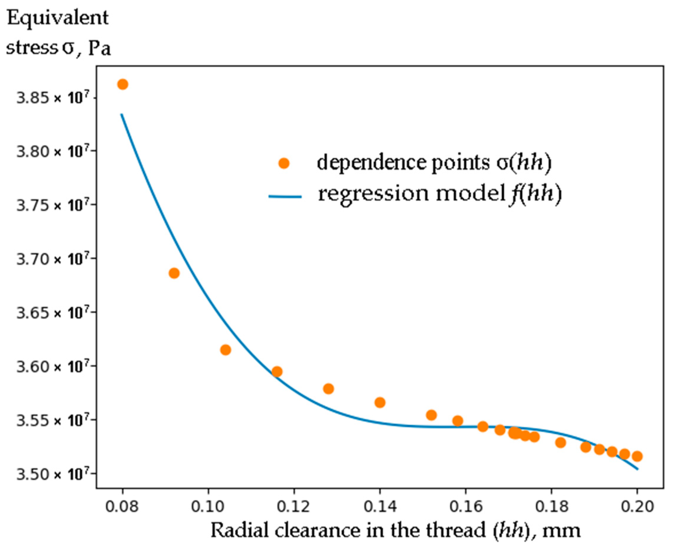
Ray is initialized first. Next, the agent environment e is created. Then, a uniform grid (array X) with six values of x in the interval [0.08, 0.2] is created. After that, agent-actors of the OptiX class are created for optimization. Each receives an FEA class agent and one value from the X array. By executing the agents’ calc() function in parallel, the y value is calculated. After that, the XY data is written to the e environment. Two additional actors of the OptiR class are created that implement another optimization method. Since they use a deterministic algorithm, they must differ in F functions. The first uses a second-degree polynomial and the second uses a third-degree polynomial. Next, the rule() function of each agent is executed until they all return None. After the completion of the calculations, we read the XY attribute of the environment and find the minimum (hh=0.2). The user can also visualize the XY points and the regression curve (Figure 9).
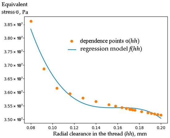
Figure 9.
Dependence points σ(hh) obtained during optimization and regression model f(hh).
Calculating the minimum of the function σ(hh) in this way on a computer with an Intel Xeon CPU E5-2630L v3 (eight cores) took 17 min, which is 5.6 times faster than the sequential execution of tasks for the 23 values of x. The maximum CPU load is 64% and RAM is 20 GB. In most cases, this optimization method allows us to immediately obtain the regression equation f(hh):
which, in the case of a high value of R2, can be formalized and placed in the knowledge base. Instead of R2, the user can apply other indicators of the model quality, for example, those obtained using cross-validation.
4. Discussion
As a rule, all system-wide regularities explored by systems theory allow the system to be more efficient. This follows from the fact of the long-term evolution of various systems in which researchers observe these regularities.
The regularities of integrity are perhaps the most important. Many successes and failures in the life cycles of complex systems can be explained by the effects of the synergy and dyssynergy of their elements. This also applies to the PLM system. For example, the combination of conceptual design tools of a construction only with process design tools seems to be dyssynergy and threatens with additional costs, since the latter require the most accurate descriptions of the construction, and not the abstract ones that are generated in large numbers by the former. However, supplementing the first tools with CAD/FEA tools can significantly reduce costs by reducing the number of unsubstantiated hypotheses. In the developed system, the emergence manifests itself in the interaction of agents of classes such as FEA and Opti, FEA and CAM, OptiX and OptiR, or various agents of the OptiR class. The regularity of integrativity is clearly visible in a system with OptiX and OptiR, which use opposite approaches to optimization. In the OptiX agent, opposite feedbacks are noticeable, created by opposite stochastic and deterministic algorithms, and together allowing to effectively overcome local minima. The “requisite variety” is manifested in the variety of types of agents used and the variety of solutions (helixPoints2() function and Opti classes). With an increase in the variety, the efficiency of the system will increase, so the user should try to expand the system with agents of a different type. This is quite easy to implement, since the behavior of the developed agents is described by relatively simple rules. Hierarchy and self-similarity is manifested in the possibility of creating hierarchical compositions of agents that are similar at different levels of the hierarchy (for example, the Opti agent composition using FEA agents). Historicity is in the presence of cyclic optimization processes with access to a higher level of quality. The developed PLM system structurally and dynamically corresponds to its environment (product life cycle). Optimization agents can be used at various stages of the life cycle. The value of the function being optimized can be returned not only by FEA agents, but also, for example, by SCADA agents that determine the performance of the product at the stage of full-scale testing or operation. This is the flexibility of agents. Nonlinearity is in the stochastic behavior of OptiX agents. Part of the self-organization can be observed in the examples of using agents for the logical inference of facts and as agents for optimization. The regularity of additivity and progressive factorization is manifested in the autonomy of agents and the possibility of a constant increase in the level of autonomy and specialization. So, at the next stage of system development, the FEA agent can be divided into three more specialized agents: geometric models, mesh generators, and solvers. Other regularities are planned to be investigated in the future.
The use of PLM system resources in the wrong place and at the wrong time, or in other words, the use for other purposes, threatens to significantly reduce the efficiency of the system. In many cases, the PLM system designer does not exactly know the purpose of a particular resource. Therefore, the system should provide mechanisms for the self-identification and self-organization of resources, for example, those described in this paper [70]. The easiest way is to endow agents with a memory mechanism in which the experience of a positive or negative interaction of the agents is stored. Then, the choice by the agent of a partner of a certain class will take into account this experience. The level of synergy of the interacting elements should be controlled on a certain scale, taking into account their hierarchy [9]. Thus, the effectiveness of the interaction can be unexpectedly high, medium, negligible, can drop to zero, or can even have devastating consequences. All developed agents can be classified according to the features of the stage of activity at which they are used, or according to other features, and pairs of classes with a high or low level of synergy can be identified [9]. The relationship class can be found using classification methods known in the field of machine learning. This is planned to be implemented in the future. In general, the system allows an application of two opposite approaches for its use: axiological (when the user formulates goals) and causal (when the goal cannot be formulated immediately, but arises as a result of the self-organization of agents).
The proposed system architecture based on the concept of actors and the use of the Ray package is not the only possible one. In the future, it is planned to be supplemented or replaced with a microservice architecture. To speed up the work of agents, the memorization technique can be used—in order to avoid re-computation with the same input data, the results are remembered. In the case of a large set of facts and rules, more productive algorithms or tools should be used, such as RETE [71] or pydatalog [31,72].
An important feature is the use of free software, which allows students and researchers to easily integrate other tools into the system and expand its capabilities. Using Python and its packages greatly facilitates this process, due to their flexibility and the easy understanding of Python code by other programmers.
More details about the project can be found on the project site on GitHub [63]. The authors propose that you join the project and leave your wishes and comments.
5. Summary and Conclusions
The principles proposed by the authors are that the basic properties of the elements, the architecture of the system, the methods of its functioning and use, and other tools should be chosen so that they correspond as much as possible to the known system-wide regularities. Compliance with these regularities must be proven at each stage of the development of a PLM system. For example, it is shown that Python provides an ease of development for components in the form of Python classes and their flexibility, in particular concerning the flexibility of knowledge representation. Knowledge can be inferred not only from triplets, but also from other agents, such as FEA or Opti. The Ray package provides an easy adaptation of the Python classes for asynchronous work. Different open-source software and Python packages provide the ability to evolve the system. Each agent has relatively simple behaviors, implemented by its rule function, and can interact with other agents. This provides the possibility of the appearance in the developed system of regularities such as emergence, historicity, “requisite variety”, and self-organization, which testifies to its effectiveness. Accordingly, the purpose of this work was achieved, and the following conclusions can be drawn:
1. Using the achievements of systems theory and the principle of isomorphism of system-wide regularities is a necessary condition for designing effective PLM systems.
2. The available open-source software makes it relatively easy to develop a multi-agent PLM system framework and components to support any stage of the product life cycle.
3. Thanks to the use of a systematic approach, an agent-oriented approach, and the high-level free tools (Python, Ray, Pycalculix, Jupyter, etc.), the proposed system has the ability to be easily studied, researched, and improved. Additional research needs to be carried out to ensure self-organization at all stages of the life cycle, taking into account the level of synergy, improving the efficiency of the existing components, and creating new components.
4. Using the developed PLM system will help to reduce time costs of the optimization processes of the life cycle, in particular, those containing the following stages: conceptual design, structural design, design of technological process, production, and testing. Based on the example above, the parallel operation of eight agents to optimize one parameter using an eight-core processor made it possible to reduce the time spent by 5.6 times. The estimated duration of the FEA-based optimization stage is 17 min, and a complete PLM activity cycle can take less than an hour, excluding the Implementation-Evaluation stage.
Author Contributions
Conceptualization, V.K.; methodology, V.K. and O.O.; software, V.K. and O.O.; validation, O.O., V.P. and P.D.; formal analysis, O.O. and C.B.; investigation, C.B., V.P. and P.D.; resources, C.B.; data curation, C.B.; writing—original draft preparation, V.K.; writing—review and editing, P.D. and C.B.; visualization, O.O.; supervision, V.P. and C.B.; project administration, O.O.; funding acquisition, C.B. All authors have read and agreed to the published version of the manuscript.
Funding
The authors are grateful to the Ministry of Education and Science of Ukraine for the grant received to implement the project D-2-22-P (RK 0122U002082).
Data Availability Statement
Not applicable.
Acknowledgments
The team of authors express their gratitude to the reviewers for their valuable recommendations that have been taken into account to significantly improve the quality of this paper.
Conflicts of Interest
The authors declare no conflict of interest.
References
- Saaksvuori, A.; Immonen, A. Product Lifecycle Management, 3rd ed.; Springer: Berlin/Heidelberg, Germany, 2008. [Google Scholar]
- Grieves, M. Product Lifecycle Management—Driving the Next Generation of Lean Thinking; McGraw-Hill: New York, NY, USA, 2006. [Google Scholar]
- Liu, W.; Zeng, Y.; Maletz, M.; Brisson, D. Product Lifecycle Management: A Survey. In Proceedings of the 29th ASME 2009 International Design Engineering Technical Conferences and Computers and Information in Engineering Conference, Parts A and B, San Diego, CA, USA, 30 August–2 September 2009; Volume 2, pp. 1213–1225. [Google Scholar]
- Kopey, V.B. Abstract model of product lifecycle management system. Precarpathian Bull. Shevchenko Sci. Soc. 2017, 2, 71–96. (In Ukrainian) [Google Scholar]
- Bertalanffy, L.V. General System Theory: Foundations, Development, Applications; George Braziller, Inc.: New York, NY, USA, 1968. [Google Scholar]
- Kossiakoff, A.; Sweet, W.N.; Seymour, S.J.; Biemer, S.M. Systems Engineering Principles and Practice, 2nd ed.; A John Wiley & Sons: Hoboken, NJ, USA, 2011. [Google Scholar]
- Volkova, V.N. Gradual Formalization of Decision-Making Models; Saint Petersburg State Technical University: Saint Petersburg, Russia, 2006. (In Russian) [Google Scholar]
- Shchedrovitsky, G.P. Selected Writings; Shkola Kul’turnoj Politiki: Moscow, Russia, 1995. (In Russian) [Google Scholar]
- Kopei, V.B. Scientific and Methodological Bases of Computer-Aided Design of Equipment for a Sucker Rod Pumping Unit. Ph.D. Thesis, Technical Sciences Degree in Speciality 05.05.12—Machines of Oil and Gas Industry. Ivano-Frankivsk National Technical University of Oil and Gas, Ivano-Frankivsk, Ukraine, 2020. (In Ukrainian). [Google Scholar]
- Wooldridge, M.; Jennings, N.R. Intelligent agents: Theory and practice. Knowl. Eng. Rev. 1995, 10, 115–152. [Google Scholar] [CrossRef]
- Wooldridge, M. An Introduction to Multi-Agent Systems; John Wiley & Sons: Hoboken, NJ, USA, 2009. [Google Scholar]
- Shoham, Y.; Leyton-Brown, K. Multiagent Systems: Algorithmic, Game-Theoretic, and Logical Foundations; Cambridge University Press: Cambridge, MA, USA, 2008. [Google Scholar]
- Kravari, K.; Bassiliades, N. A survey of agent platforms. J. Artif. Soc. Soc. Simul. 2015, 18, 11. [Google Scholar] [CrossRef]
- Shoham, Y. Agent-oriented programming. Artif. Intell. 1993, 60, 51–92. [Google Scholar] [CrossRef]
- Abadi, A.; Sekkat, S.; Zemmouri, E.M.; Benazza, H. Using Ontologies for the Integration of Information Systems Dedicated to Product (CFAO, PLM…) and Those of Systems Monitoring (ERP, MES..). In Proceedings of the 2017 International Colloquium on Logistics and Supply Chain Management, LOGISTIQUA 2017, Rabat, Morocco, 27–28 April 2017; pp. 59–64. [Google Scholar]
- Camarillo, A.; Ríos, J.; Althoff, K. Knowledge-based multi-agent system for manufacturing problem solving process in production plants. J. Manuf. Syst. 2018, 47, 115–127. [Google Scholar] [CrossRef]
- Reichle, M.; Bach, K.; Althoff, K.D. The Seasalt Architecture and Its Realization within the Docquery Project. In KI 2009, Advances in Artificial Intelligence; Springer: Berlin/Heidelberg, Germany, 2009; pp. 556–563. [Google Scholar]
- Diakun, J.; Dostatni, E. End-of-life design aid in PLM environment using agent technology. Bull. Pol. Acad. Sci. Tech. Sci. 2020, 68, 207–214. [Google Scholar]
- Dostatni, E.; Diakun, J.; Hamrol, A.; Mazur, W. Application of agent technology for recycling-oriented product assessment. Ind. Manag. Data Syst. 2013, 113, 817–839. [Google Scholar] [CrossRef]
- Gomes, S.; Monticolo, D.; Hilaire, V.; Mahdjoub, M. A multi-agent system embedded to a product lifecycle management to synthesise and reuse industrial knowledge. Int. J. Prod. Lifecycle Manag. 2007, 2, 317–336. [Google Scholar] [CrossRef]
- Kumar, V.V.; Sahoo, A.; Liou, F.W. Cyber-enabled product lifecycle management: A multi-agent framework. Procedia Manuf. 2019, 39, 123–131. [Google Scholar] [CrossRef]
- Lahoud, I.; Gomes, S.; Hilaire, V.; Monticolo, D. A Multi-Agent Platform to Manage Distributed and Heterogeneous Knowledge by Using Semantic Web. In Proceedings of the IAENG Transactions on Electrical Engineering Volume 1: Special Issue of the International Multiconference of Engineers and Computer Scientists 2012, Hong Kong, China, 14–16 March 2012; pp. 215–228. [Google Scholar]
- Mahdjoub, M.; Monticolo, D.; Gomes, S.; Sagot, J. A collaborative design for usability approach supported by virtual reality and a multi-agent system embedded in a PLM environment. CAD Comput. Aided Des. 2010, 42, 402–413. [Google Scholar] [CrossRef]
- Marchetta, M.G.; Mayer, F.; Forradellas, R.Q. A reference framework following a proactive approach for product lifecycle management. Comput. Ind. 2011, 62, 672–683. [Google Scholar] [CrossRef]
- Matsokis, A.; Kiritsis, D. An ontology-based approach for product lifecycle management. Comput. Ind. 2010, 61, 787–797. [Google Scholar] [CrossRef]
- Choiński, D.; Senik, M. Distributed control systems integration and management with an ontology-based multi-agent system. Bull. Pol. Acad. Tech. 2018, 5, 613–620. [Google Scholar]
- Karasev, V.O.; Sukhanov, V.A. Product lifecycle management using multi-agent systems models. Procedia Comput. Sci. 2017, 103, 142–147. [Google Scholar] [CrossRef]
- Giret, A.; Botti, V. From System Requirements to Holonic Manufacturing System Analysis. Int. J. Prod. Res. 2006, 44, 3917–3928. [Google Scholar] [CrossRef]
- Derigent, W.; Cardin, O.; Trentesaux, D. Industry 4.0: Contributions of holonic manufacturing control architectures and future challenges. J. Intell. Manuf. 2020, 32, 1797–1818. [Google Scholar] [CrossRef]
- Bussmann, S.; Jennings, N.R.; Wooldridge, M. Multiagent Systems for Manufacturing Control: A Design Methodology; Springer: Berlin/Heidelberg, Germany, 2004. [Google Scholar]
- Kopei, V.B.; Onysko, O.R.; Panchuk, V.G. Principles of development of product lifecycle management system for threaded connections based on the Python programming language. J. Phys. Conf. Ser. 2020, 1426, 012033. [Google Scholar] [CrossRef]
- Birger, I.A.; Iosilevich, G.B. Threaded and Flange Connections; Mashinostroenie: Moscow, Russia, 1990. (In Russian) [Google Scholar]
- Bickford, J.H. An Introduction to the Design and Behavior of Bolted Joints, 3rd ed.; Revised and Expanded; CRC Press: Taylor and Francis: Boca Raton, FL, USA, 2017. [Google Scholar]
- Fukuoka, T. The Mechanics of Threaded Fasteners and Bolted Joints for Engineering and Design; Elsevier: Amsterdam, The Netherlands, 2022. [Google Scholar]
- Shatskyi, I.; Ropyak, L.; Velychkovych, A. Model of contact interaction in threaded joint equipped with spring-loaded collet. Eng. Solid Mech. 2020, 8, 301–312. [Google Scholar] [CrossRef]
- Tutko, T.; Dubei, O.; Ropyak, L.; Vytvytskyi, V. Determination of Radial Displacement Coefficient for Designing of Thread Joint of Thin-Walled Shells. In Lecture Notes in Mechanical Engineering; Advances in Design, Simulation and Manufacturing IV. DSMIE 2021; Ivanov, V., Trojanowska, J., Pavlenko, I., Zajac, J., Peraković, D., Eds.; Springer: Cham, Switzerland, 2021; pp. 153–162. [Google Scholar]
- Dubei, O.Y.; Tutko, T.F.; Ropyak, L.Y.; Shovkoplias, M.V. Development of Analytical Model of Threaded Connection of Tubular Parts of Chrome-Plated Metal Structures. Metallofiz. Noveishie Tekhnologii 2022, 44, 251–272. [Google Scholar] [CrossRef]
- Pryhorovska, T.; Ropyak, L. Machining Error Influence on Stress State of Conical Thread Joint Details. In Proceedings of the International Conference on Advanced Optoelectronics and Lasers, CAOL, Sozopol, Bulgaria, 6–8 September 2019; pp. 493–497. [Google Scholar] [CrossRef]
- Bazaluk, O.; Velychkovych, A.; Ropyak, L.; Pashechko, M.; Pryhorovska, T.; Lozynskyi, V. Influence of heavy weight drill pipe material and drill bit manufacturing errors on stress state of steel blades. Energies 2021, 14, 4198. [Google Scholar] [CrossRef]
- Ropyak, L.Y.; Vytvytskyi, V.S.; Velychkovych, A.S.; Pryhorovska, T.O.; Shovkoplias, M.V. Study on grinding mode effect on external conical thread quality. IOP Conf. Ser. Mater. Sci. Eng. 2021, 1018, 012014. [Google Scholar] [CrossRef]
- Neshta, A.; Kryvoruchko, D.; Hatala, M.; Ivanov, V.; Botko, F.; Radchenko, S.; Mital, D. Technological Assurance of High-Efficiency Machining of Internal Rope Threads on Computer Numerical Control Milling Machines. J. Manuf. Sci. Eng. 2018, 140, 071012. [Google Scholar] [CrossRef]
- Shats’kyi, I.P.; Lyskanych, O.M.; Kornuta, V.A. Combined Deformation Conditions for Fatigue Damage Indicator and Well-Drilling Tool Joint. Strength Mater. 2016, 48, 469–472. [Google Scholar] [CrossRef]
- Severinchik, N.A.; Kopei, B.V. Inhibitive protection of steel drill pipes from corrosion fatigue. Sov. Mater. Sci. 1978, 13, 318–319. [Google Scholar] [CrossRef]
- Kopei, B.V.; Gnyp, I.P. A method for the prediction of the service life of high-strength drill pipes based on the criteria of corrosion fatigue. Mater. Sci. 1997, 33, 99–103. [Google Scholar] [CrossRef]
- Van Rossum, G.; Drake, F.L. Python 3 Reference Manual; CreateSpace: Scotts Valley, CA, USA, 2009. [Google Scholar]
- Artamonov, I.V. Free software: Advantages and disadvantages. Izv. Irkutsk. State Econ. Acad. 2012, 5, 122–125. (In Russian) [Google Scholar]
- Dhondt, G. The Finite Element Method for Three-Dimensional Thermomechanical Applications; Wiley: Hoboken, NJ, USA, 2004. [Google Scholar]
- Geuzaine, C.; Remacle, J.F. Gmsh: A Three-Dimensional Finite Element Mesh generator with built-in pre- and post-processing facilities. Int. J. Numer. Methods Eng. 2009, 79, 1309–1331. [Google Scholar] [CrossRef]
- Fritzson, P.; Aronsson, P.; Lundvall, H.; Nyström, K.; Pop, A.; Saldamli, L.; Broman, D. The OpenModelica Modeling, Simulation, and Software Development Environment. Simul. News Eur. Dec. 2005, 15, 8–16. [Google Scholar]
- Grbl: An Open Source, Embedded, High Performance g-Code-Parser and CNC Milling Controller Written in Optimized C That Will Run on a Straight Arduino. Available online: https://github.com/gnea/grbl (accessed on 29 December 2022).
- Paviot, T. Pythonocc-Core: Python Package for 3D CAD/BIM/PLM/CAM. Available online: https://github.com/tpaviot/pythonocc-core (accessed on 29 December 2022).
- OPEN CASCADE. Available online: http://www.opencascade.com (accessed on 29 December 2022).
- FreeCAD: Your Own 3D Parametric Modeler. Available online: https://www.freecadweb.org (accessed on 29 December 2022).
- Harris, C.R.; Millman, K.J.; van der Walt, S.J.; Gommers, R.; Virtanen, P.; Cournapeau, D.; Wieser, E.; Taylor, J.; Berg, S.; Smith, N.J.; et al. Array programming with NumPy. Nature 2020, 585, 357–362. [Google Scholar] [CrossRef]
- Virtanen, P.; Gommers, R.; Oliphant, T.E.; Haberland, M.; Reddy, T.; Cournapeau, D.; Burovski, E.; Peterson, P.; Weckesser, W.; Bright, J.; et al. SciPy 1.0: Fundamental Algorithms for Scientific Computing in Python. Nat. Methods 2020, 17, 261–272. [Google Scholar] [CrossRef]
- Hunter, J.D. Matplotlib: A 2D graphics environment. Comput. Sci. Eng. 2007, 9, 90–95. [Google Scholar] [CrossRef]
- Meurer, A.; Smith, C.P.; Paprocki, M.; Čertík, O.; Kirpichev, S.B.; Rocklin, M.; Kumar, A.; Ivanov, S.; Moore, J.K.; Singh, S.; et al. SymPy: Symbolic computing in Python. PeerJ Comput. Sci. 2017, 3, e103. [Google Scholar] [CrossRef]
- Pedregosa, F.; Varoquaux, G.; Gramfort, A.; Michel, V.; Thirion, B.; Grisel, O.; Blondel, M.; Prettenhofer, P.; Weiss, R.; Dubourg, V.; et al. Scikit-learn: Machine learning in Python. JMLR 2011, 12, 2825–2830. [Google Scholar]
- Black, J. Pycalculix. Available online: https://github.com/spacether/pycalculix (accessed on 29 December 2022).
- Kluyver, T.; Ragan-Kelley, B.; Pérez, F.; Granger, B.; Bussonnier, M.; Frederic, J.; Bussonnier, M.; Frederic, J.; Kelley, K.; Hamrick, J.; et al. Jupyter Notebooks—A Publishing Format for Reproducible Computational Workflows. In Positioning and Power in Academic Publishing: Players, Agents and Agendas; Loizides, F., Scmidt, B., Eds.; IOS Press: Amsterdam, The Netherlands, 2016; pp. 87–90. [Google Scholar]
- Moritz, P.; Nishihara, R.; Wang, S.; Tumanov, A.; Liaw, R.; Liang, E.; Elibol, M.; Yang, Z.; Paul, W.; Jordan, M.I.; et al. Ray: A Distributed Framework for Emerging AI Applications. In Proceedings of the 13th USENIX Symposium on Operating Systems Design and Implementation (OSDI’18), Carlsbad, CA, USA, 8–10 October 2018. [Google Scholar]
- Rogers, D.F.; Adams, J.A. Mathematical Elements for Computer Graphics, 2nd ed.; McGraw-Hill: New York, NY, USA, 1989. [Google Scholar]
- Kopei, V.; Onysko, O. Educational Multi-Agent PLM System for Threaded Connections. Available online: https://github.com/vkopey/ThreadsPLM-MAS (accessed on 31 December 2022).
- CLIPS: A Tool for Building Expert Systems. Available online: https://clipsrules.net (accessed on 29 December 2022).
- Python Streaming Scripts. Available online: https://github.com/gnea/grbl/wiki/Using-Grbl#python-streaming-scripts-officially-supported-by-grbl-cross-platform (accessed on 29 December 2022).
- GRBL Controller Application with G-Code Visualizer Written in Qt. Available online: https://github.com/Denvi/Candle (accessed on 29 December 2022).
- PCB Design and Circuit Simulator Software—Proteus. Available online: https://www.labcenter.com (accessed on 29 December 2022).
- Wales, D.J.; Doye, J.P.K. Global Optimization by Basin-Hopping and the Lowest Energy Structures of Lennard-Jones Clusters Containing up to 110 Atoms. J. Phys. Chem. A 1997, 101, 5111. [Google Scholar] [CrossRef]
- Storn, R.; Price, K. Differential Evolution—A Simple and Efficient Heuristic for Global Optimization over Continuous Spaces. J. Glob. Optim. 1997, 11, 341–359. [Google Scholar] [CrossRef]
- Kopei, V.B. Algorithm of an Intelligent System Based on Interdisciplinary Studies of System-Wide Regularities. In Proceedings of the Materials 4th International Scientific-Technical Conference Computer Modelling and Optimization of Complex System, Ministry of Education and Science of Ukraine, Ukrainian State University of Chemical Technology, Balance-Club, Dnipro, Ukraine, 1–2 November 2018; pp. 246–248. (In Ukrainian). [Google Scholar]
- Forgy, C. Rete: A Fast Algorithm for the Many Pattern/Many Object Pattern Match Problem. Artif. Intell. 1982, 19, 17–37. [Google Scholar] [CrossRef]
- Datalog Logic Programming in Python. Available online: https://sites.google.com/site/pydatalog (accessed on 29 December 2022).


Disclaimer/Publisher’s Note: The statements, opinions and data contained in all publications are solely those of the individual author(s) and contributor(s) and not of MDPI and/or the editor(s). MDPI and/or the editor(s) disclaim responsibility for any injury to people or property resulting from any ideas, methods, instructions or products referred to in the content. |
© 2023 by the authors. Licensee MDPI, Basel, Switzerland. This article is an open access article distributed under the terms and conditions of the Creative Commons Attribution (CC BY) license (https://creativecommons.org/licenses/by/4.0/).