Abstract
Electrical machines generate unwanted flux and current harmonics. Harmonics can be suppressed using various methods. In this paper, the harmonics are significantly reduced using Iterative Learning Control (ILC) and Neural Networks (NNs). The ILC can compensate for the harmonics well for operation at constant speed and current reference values. The NNs are trained with the data from the ILC and help to suppress the harmonics well even in transient operation. The simulation model is based on flux and torque maps, depending on -currents and the electrical angle. The maps are generated from FEM simulation of an interior permanent magnet synchronous machine (IPM) and are published with the paper. They are intended to serve other researchers for direct comparison with their own methods. Simulation results in this paper verify that by using ILC and NNs together, current harmonics in transient operation can be eliminated better than without NNs.
Keywords:
PMSM; PSM; iterative learning control; repetitive control; harmonics; neural networks; FOC 1. Introduction
Current harmonics are a prominent issue in permanent magnet synchronous machines (PMSMs) used in industrial and traction drive applications. These harmonics cause power losses and reduce the efficiency of PMSMs. Current harmonics can be caused by various factors, including the switching behavior or nonlinearities of the inverter [], but also the flux and torque harmonics. There is extensive research on the topic of compensating inverter switching dead time harmonics that explores various techniques and approaches for compensating the harmonics caused by switching dead time. These methods involve data-intensive approaches where compensation voltage values are extracted from lookup tables (LUTs) [], as well as the utilization of observers [] and other methods that require careful parameter tuning []. All of these techniques are specifically employed to achieve effective dead time compensation.
This paper focuses on eliminating flux harmonics as the cause of current harmonics. Flux harmonics within the motor generate current harmonics [], which can be detected as phase current harmonics. When the alternating phase currents are transformed into direct -currents in field-oriented control, harmonics cause a distortion by adding an alternating component to the direct currents. Previous research has applied methods such as additional PI controllers, state controllers, or ILC using a 2D array to map the correction signal for different speeds [] or a speed-independent mapping in one vector [] to eliminate current harmonics. However, these implementations are less effective at rapidly changing speeds and cannot map harmonics that change with torque or changing -currents, or are not as accurate at constant speed and torque values [].
This research focuses on minimizing flux harmonics for both changing and constant operating values using iterative learning control (ILC) and neural networks (NNs) to eliminate harmonics in PMSMs. ILC can reduce periodic errors by storing and processing the error of the last period, while NNs can learn, find a pattern, and interpolate from the data to provide an accurate solution.
The method is tested in simulations using MATLAB, and the results demonstrate that the approach effectively eliminates current harmonics. The simulation model is based on data generated using finite element method simulation. Flux and torque are considered as a function of both the -currents and the electrical rotor angle. The flux and torque maps can be downloaded along with this paper for further analysis. The model background as well as the benchmark motor will be described further in the next section, followed by the more detailed description of the control method and the simulation results.
2. Current Research
This section provides a brief overview of current research in the area, divided into subsections on iterative learning control, machine learning, and harmonic minimization.
2.1. Iterative Learning Control
Recent research uses ILC for a variety of tasks such as friction correction, trajectory or position tracking, voltage stabilization, or to adjust control quantity. Riaz et al. [] employ ILC to correct friction at low speeds, while [] utilized it for trajectory tracking of pneumatic muscle actuators with state constraints. Suh et al. [] propose a current-error-based ILC approach with a nonlinear controller to improve position-tracking performance in permanent magnet stepper motors. Angalaeswari et al. [] apply ILC in both autonomous and grid-connected modes with varying generation and loading conditions to maintain stable voltage and frequency in a microgrid. In [], Yang et al. present a discrete iterative learning control algorithm that incorporates error backward association to adjust the control quantity for the subsequent iteration.
ILC has the capability to reduce repetitive or periodic errors. Fei et al. [] combine Model Predictive Control (MPC) with ILC to enhance system response time and reduce speed fluctuations. ILC can also be applied for suppressing rotor position harmonics errors in sensorless PMSM drives [], or to counteract the influence of periodic and nonperiodic disturbances in a three-phase constant-voltage constant-frequency standalone voltage source inverter (VSI) with an LC filter, even under variable initial conditions [].
2.2. Machine Learning and Neural Networks in Power Electronics
Machine learning and neural networks are already widely used in power electronics for applications including system modeling, design, control, and maintenance. Patan et al. [] employ neural networks (NNs) in their ILC approach to model the inverse system and use it for reference tracking with a nonlinear pneumatic servomechanism. In addition to ILC, machine learning has found applications in various areas of power electronics. Zhao et al. [] present a comprehensive overview of published applications of machine learning in power electronics, highlighting the significant increase in research in recent years. In their literature review, Zhao et al. divide the applications of artificial intelligence (AI) in power electronics into three aspects: design, control, and maintenance. Four categories of AI are discussed, namely expert systems, fuzzy logic, metaheuristic methods, and machine learning. The functions of AI are further divided into optimization, classification, regression, and data structure exploration, with optimization and regression being the most widely applied []. The NNs used in this paper could be categorized as a control application, machine learning, and regression.
Zhang et al. [] provide a narrower review of the existing literature on the use of machine learning for controlling and monitoring electric machine drives. They divide their research into ML applications for induction machines, PMSMs, inverters, and sensors; reinforcement learning algorithms; and embedded platforms used to apply ML on the testbench [].
There are also other reviews available that specifically focus on the use of neural networks in power electronics, such as those by Bose et al. [,]. The growing body of research concerning machine learning in power electronics demonstrates the high level of interest within the research community.
2.3. Motor Harmonic Minimization
Flux and torque harmonics in motors are influenced by the motor design and can be mitigated by appropriate design choices [], but often are not. When optimal motor design is not feasible for reducing harmonics, effective control techniques can provide assistance. Torque harmonics contribute to torque and speed fluctuations, which can be mitigated using ILC, also referred to as repetitive control (RC), in various ways [,,]. Pei et al. [] utilize a P-type ILC to decrease speed ripple. ILC can also be used to reduce the harmonics on the phase currents [,]. Another method to reduce flux harmonics, which manifest as current harmonics, involves injecting voltage harmonics []. In a direct comparison between ILC, a PI-controller-based method, and a state space controller, ILC demonstrated the best compensation performance among the three methods for constant speed and constant current reference values []. However, in transient operations, the other methods outperformed ILC []. This paper combines ILC with NNs to enhance performance, particularly during transient operation.
3. Nonlinear Drive System Model
3.1. Model Background
The system under control in this scenario consists of a permanent magnet synchronous machine (PMSM) and an inverter. The voltage equations of the PMSM have been transformed into the -system using the Clarke–Park transformation, and these well-known linear model equations are presented in Equation (1) [].
In this system, and denote the -axis voltages and currents, respectively. represents the stator resistance, and is the electric angular velocity, which can be calculated based on the speed and the number of pole pairs. refers to the stator magnetic fluxes in the axes, while represents the magnetic flux of the permanent magnets. denotes the components of the inductance of the stator winding.
The linear motor model with constant inductances provides an approximation of the motor, but only to a certain extent, as it does not take into account the effects of iron saturation. To obtain more accurate results, the model used for this study is extended to include data on saturation. As a result, the inductances are taken to depend on the load and, therefore, on the -currents []. Consequently, the magnetic field is no longer linearly dependent on the current []. To represent flux and torque harmonics, both flux and torque are considered to be angle-dependent, with the electrical rotor angle serving as the corresponding angle. Cross-saturation also contributes to the nonlinearity of the motor and affects the inductances. Simplifying assumptions include the symmetry of the three phases and the absence of a connected star point in the machine, as outlined in []. It should be noted that temperature also affects motor parameters such as stator resistance and could be measured using appropriate sensors, although this aspect is not discussed further in this work. This research uses the current-dependent fluxes to represent saturation.
Using the equations provided, the block diagram shown in Figure 1 can be constructed. The model considers the angular dependence of flux and torque as shown in Figure 1.
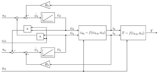
Figure 1.
Block diagram of the PMSM machine model used for simulations where the functions for the -currents and the torque are mapped from look-up tables of the benchmark motor.
The fluxes, currents, and torques mapped are therefore non-linearly dependent. The functions of the -currents and the torque are mapped using look-up tables (LUTs). The data for the LUTs were obtained from a finite element method (FEM) simulation. The simulated motor is described in the next section.
3.2. Benchmark Motor
The electric motor used in the simulations has 24 stator slots and 16 poles. This slot–pole combination and the slot effect result in harmonics, which are accurately simulated using FEM software. The electric motor and its flux density distribution are illustrated in Figure 2.
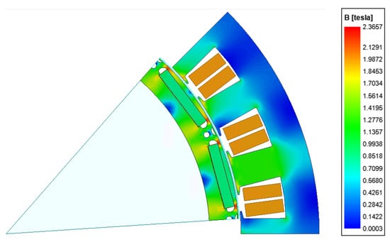
Figure 2.
Illustration of the electric machine and its flux density distribution.
The electric motor was designed as a traction drive and its efficiency map was calculated. As depicted in Figure 3, the simulated machine’s base speed registered at 3000 rpm, with a maximum speed of 7000 rpm, and the Interior Permanent Magnet (IPM) showcasing an approximate maximum efficiency of 97%. The simulation took different aspects into account; the mechanical tensile strength of the rotor sheets was tested, and the thermal behavior was considered in the design. However, this paper focuses on the discussion of harmonics and will not go into detail on the mechanical results. The key parameters of the electric machine are outlined in Table 1.
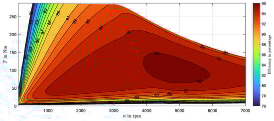
Figure 3.
Efficiency map over speed and torque; efficiencies less than 75% in the upper left corner and at the bottom are not plotted to obtain a better color distribution.

Table 1.
Linear PMSM motor parameters used for controller parameterization and simulation.
Figure 4 displays the interdependencies between the magnetic -fluxes and the current on the -axis, along with the associated -inductances on the -axis. The fluxes and inductances presented here are averaged over an electrical period; for the simulation, these data were taken into account depending on the electrical angle.
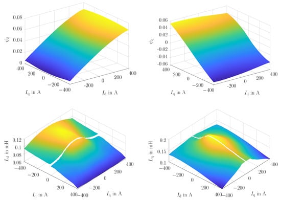
Figure 4.
Magnetic -fluxes , and -inductances , of the benchmark motor on the -axis averaged over an electrical period.
4. Control Architecture
The fundamental control architecture utilized in this study is based on field-oriented control (FOC). In this control approach, the phase currents are transformed into -currents using the transformation method described earlier. The -current setpoints and actual values are then processed by PI controllers to generate corresponding -voltages. These -voltages are subsequently transformed back into phase voltages using inverse Park–Clarke transformation to determine the duty cycle for the inverter. The PI controllers are tuned using the magnitude optimum method. To suppress current harmonics, correction signals are added to the -current setpoints utilizing current harmonic suppression controllers, such as the ILC.
The ILC is further enhanced and emulated using neural networks, as described in subsequent sections.
4.1. Iterative Learning Control
The ILC method used in this study is consistent with previous literature [,] and is similar to the approach presented in [,]. In the context of iterative learning control, it is crucial to differentiate between repeated cyclic and periodically cyclic processes. This research considers only periodically cyclic processes and all concepts in this section are based on [] unless otherwise stated.
A signal is considered periodically cyclic if , where N is the fixed number of samples within a single period. The value of N corresponds to the length of the periodically cyclic process, and if controlling a PMSM, it represents the samples per electrical rotation and is dependent on the motor’s speed and sampling time .
The iterative learning control signal in the next pass () corresponds to the one in the current pass added to the weighted correction, as described in Equation (6).
represents the controller output signal, and denotes a correcting signal formed by the convolution of the error signal and the impulse response of the inverse system transfer function . The learning factor weights and therefore determines the learning speed.
At or , the ILC is unstable, and at , the ILC learns fastest []. The z-transformation of Equation (6) leads to Equation (7):
where is the period filter and the transfer function from to is called loop filter .
In Figure 5, represents the system on which the disturbance , in this case the harmonics, acts. The loop filter is set equal to the inverse transfer function of the system, i.e., . The green section represents the ILC, while the red section represents the system on which it acts.
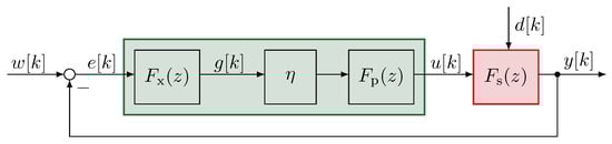
Figure 5.
Block representation of an iterative loop from [].
4.2. Iterative Learning Control in Field-Oriented Control
The ILC discussed in Section 4.1 has been integrated into the field-oriented control structure. This application implements the period filter as a ring buffer. This ring buffer stores the correction signal. Since the correction signal does not depend on the time but on the angle, the ring buffer stores the correction signal over the electrical angle . If the stored discrete angle value is not exactly met, the interpolation method described in [] is employed for reading from the ring buffer and for writing to it.
Figure 6 depicts the simplified block diagram of the ILC implemented as a current harmonics suppressor, along with the current controller. The area marked red represents the system considered for designing the ILC, as shown in Figure 5.
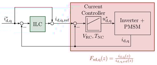
Figure 6.
Simplified block diagram of the ILC integrated into the FOC.
The system includes the closed loop of the current controller, inverter, and motor. The ILC block marked in green corresponds to the green area in Figure 5. Because the correction signal provided by the ILC is delayed relative to the changing reference currents, the reference values are added directly to the correction signal for improved dynamics.
The ILC ring buffer size is equal to N, which indicates the number of samples per electrical rotation. Since the method is to be operated for changing speeds, N also changes. The change in N would result in a change in the size of the ring buffer as well. A solution to this issue has already been proposed in previous research [,].
Instead of using only one ring buffer, ring buffers of different sizes are used for different speeds. Interpolation is then performed between these different ring buffers for the different speeds. The interpolation was found to be less effective when applied to highly variable speeds []. It is also worth noting that the harmonics may vary with the different -current combinations. Thus, even when approaching the same operating point, the harmonics must be relearned for each setpoint torque. To address these challenges, a new concept is introduced in the following section that involves utilizing neural networks to train the ILC correction signals for various operating points, i.e., -current combinations at different speeds.
4.3. Neural Networks Mapping the ILC
The neural networks utilized in this study are multi-layer perceptron (MLP) networks. The NNs are fully connected feedforward networks with hyperbolic tangent sigmoid activation functions in the hidden layers, as shown in Equation (8).
To collect data, the ILC is applied to different -current combinations along the Maximum Torque Per Current (MTPC) curve at different speeds. The correction signals, along with the reference values for the -currents and the speed, are recorded and stored. The neural networks (NNs) are trained offline; they are trained once using the previously collected data and remain unchanged during operation.
4.3.1. Variant 1: Direct ILC Mapping
For variant 1, the input consists of the reference torque , the speed , and the electrical rotor angle . To obtain a continuous angle signal, the sine and cosine of the angle are used as input, as depicted in Figure 7. The correction signals recorded for and over the electrical rotor angle are designated as targets for the NNs. The two resulting NNs, one for and the other for , can be used as a direct replacement for the ILC. Their output signals, similar to those of the ILC, are added to the reference currents.
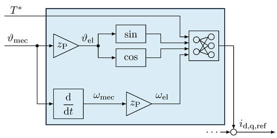
Figure 7.
Block diagram of the inputs and outputs of the NNs in variant 1.
Figure 7 illustrates how the inputs of the NN are determined from the reference currents and the mechanical rotor angle. The NNs directly output the correction signal, which is added to the reference currents. Depending on the application, the ILC correction may also be added at this point.
4.3.2. Variant 2: Frequency Mapping
In variant 2, instead of directly using the correction signals as in variant 1, a Fourier analysis (FFT) of the correction signals is calculated. The NNs then map the frequency spectrum of the correction signal. As inputs, the NNs only require the reference torque and speed, not the angle. The outputs are the amplitudes and phases for the harmonics of the correction signal. Again, for a continuous phase signal, the sine and cosine of the phases are used.
The phase and amplitude of the less pronounced or absent harmonics do not follow the same pattern over torque and speed as the more pronounced harmonics. Due to the physical structure of PMSMs, only certain harmonics are relevant. The NNs can be chosen significantly smaller if irrelevant harmonics are not mapped. Therefore, only relevant harmonics above a certain amplitude level are mapped in the NNs. The NNs have h outputs, where h is the number of frequencies mapped.
Individual NNs are trained for each of the different output signals. Thus, smaller NNs could be used. Six NNs are utilized, three each for the correction to and three for the correction to , with outputs for amplitudes, cosine of phases, and sine of phases as shown in Figure 8. The actual correction signals are then calculated from these outputs.
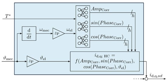
Figure 8.
Block diagram of the inputs and outputs of the NNs in variant 2.
While variant 2 requires more NNs, these NNs are considerably smaller and have fewer weights to be trained compared to the NNs in variant 1.
Figure 8 illustrates how the inputs of the NN are determined from the reference currents and the mechanical rotor angle for variant 2. The NNs still compute the correction signal, as in variant 1. Additionally, the ILC correction can also be incorporated here.
4.4. ILC in Combination with NNs
Since the NNs are trained offline, they cannot adapt to changes during operation. For this reason, the NNs are used together with the ILR in the following. The NNs can also further map the correlation of the correction signal between the reference torque and the speed for faster changes. The ILC can compensate for small changes, especially at stationary operating points.
Figure 9 displays the simplified block diagram of the ILC in combination with the NNs. The green block corresponds to the green marked part of one of the two variants from Figure 7 and Figure 8.
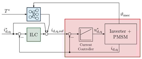
Figure 9.
Simplified block diagram of the ILC together with the NNs in the FOC.
4.5. Process Overview
The process from ILC to its combination with NNs can be divided into several steps; these are shown in Figure 10.
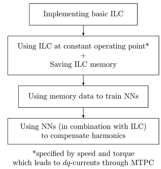
Figure 10.
Steps in the ILC and NN implementation process.
Figure 10 shows the steps needed to use NNs in combination with ILC.
Step 1. The process begins with the implementation of the ILC. The first step is to determine the inverse transfer function of the system that is to be controlled. This inverse transfer function provides the parameters for the ILC. Additionally, memory is allocated to the ILC, allowing for external access.
Step 2. The ILC is exposed to errors for multiple rotations at operation points with constant values. These operating points are selected at different speeds and torques. The MTPC curve is used to provide the required -currents for the specific torques. When the ILC has learned how to minimize the error at a specific operation point, the ILC data are collected and stored.
Step 3. Once enough data are collected to map the desired area, the data are used to train the NNs in the two variants described in Section 4.3.1 and Section 4.3.2.
Step 4. The trained NNs are used to minimize harmonics alone or in combination with the ILC, as described in Section 4.4.
5. Simulation Results and Discussion
To facilitate the comparison of the simulation outcomes for the various harmonic suppression variants outlined in Section 4, the Root Mean Squared Error (RMSE), as depicted in Equation (9), is employed. The RMSE is advantageous because it can be utilized for changing operating points as well.
The structure of the simulation model aligns with the block diagram presented in Figure 9. The current controller is implemented as a PI controller and designed according to the magnitude optimum. For the PMSM, the implementation followed the configuration shown in Figure 1. The inverter is simplified in the model as a delay unit, disregarding individual switch models.
The following subsections compare first simulation results for a constant operating point, where the frequency spectrum is also calculated. Subsequently, results for either variable speed, variable torque, or both are presented.
Variant 1 implements two NNs with three hidden layers, each with 50 neurons. The inputs for these NNs are the sine and cosine of the electrical rotor angle, the linearly calculated torque, and the current speed. The outputs are the correction signals for and .
Variant 2 employs six neural networks with two hidden layers, each composed of five neurons. These networks only take the reference torque and the current speed as inputs. Their outputs are the amplitude, cosine, and sine of the phase of the harmonics of the two correction signals, respectively. For , six harmonics are mapped (6, 12, 18, 24, 42, 48), while for , five harmonics are considered (6, 12, 18, 24, 48).
The ILC has 20 ring buffers for a speed range from 150 rpm to 3000 rpm. The training data for the NNs are generated for these 20 speeds and 40 torque values, each ranging from −344 Nm to 330 Nm along the MTPC line.
5.1. Constant Speed, Constant Torque
To compare at a constant operating point, a speed is chosen that lies between two speeds in the ILC memory and thus also between the training data of the NNs. The torque is also selected to be between two torques for which the NNs were trained. The selected operating point is at rpm and Nm. To analyze the harmonics of this operating point with and without reduction methods, a Fast Fourier analysis of the phase current is calculated, as shown in Figure 11.
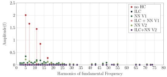
Figure 11.
Frequency spectrum of one phase current without fundamental wave component for the different controllers: Constant speed n = 820 rpm, constant torque T = 65 Nm.
Figure 11 shows the frequency spectrum of one phase current for the different methods at the selected operating point. The fundamental wave is omitted for the sake of displayability, and the harmonics are plotted as multiples of the fundamental along the x-axis. Harmonics with amplitudes less than 0.01 for all methods are not plotted for better readability. The frequency spectrum shows that in the simulated motor, the fifth and seventh harmonics, as well as the eleventh and thirteenth harmonics, are present in the phase current. All methods shown can significantly reduce these harmonics, but the methods with ILC achieve particularly good results.
A similar picture is shown by the RMSE (see Figure 12 and Table A1), calculated over 0.2 s of the -currents. All five methods can significantly reduce the RMSE. The variants with ILC perform best by far, but the difference between the different ILC variants is marginal.
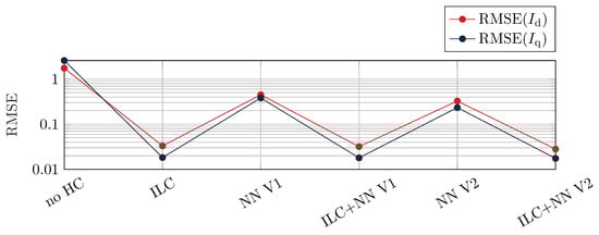
Figure 12.
RMSE calculated from -currents for the different controllers: Constant speed n = 820 rpm, constant torque T = 65 Nm.
Figure 13 shows the -currents for the different methods. The currents without harmonic reduction in subplot (a) illustrate the pronounced current harmonics in the simulated machine. Subplot (b) displays the currents with ILC, which are almost constant, similar to those in subplots (d) and (f), which represent the results of the combinations of ILC and NNs. If only the NNs are used here, some residual oscillation remains; see subplots (c) and (e). For this operating point, only a minor advantage of the combination of ILC and NNs can be shown, since here the ILC alone already produces very good results.
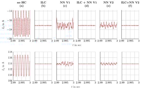
Figure 13.
-currents for the different controllers: constant speed n = 820 rpm, constant torque T = 65 Nm.
5.2. Variable Speed, Constant Torque
This subsection shows a comparison of variable speeds ranging from 500 rpm to 3000 rpm at a rate of 30,000 , with corresponding data collected for the 17th ramp. It is important to note that the methods using ILC were fully trained using 16 ramps. Due to the continuous change in speed, it is not possible to perform a Fast Fourier analysis. However, the RMSE values for the -currents are still informative and can be seen in Figure 14 and Table A1.
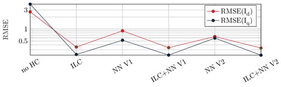
Figure 14.
RMSE calculated from -currents for the different controllers: variable speed n = 500 rpm to 3000 rpm, constant torque T = 65 Nm.
Figure 14 and Table A1 present the RMSE values for the -currents over a speed ramp ranging from 500 rpm to 3000 rpm and then back to 500 rpm, which corresponds to a duration of 0.166 s. As observed with the constant operating point, the ILC methods continue to outperform the NN methods. When the torque remains constant, the harmonics across the different speeds can be effectively mapped within the ILC memory. The gap between the performance of the ILC and non-ILC methods is not as significant as with the constant operating point.
The differences between the ILC methods are small but can be seen in the -currents in Figure 15. Subplot (a) depicts the current waveforms without harmonic suppression, revealing that the amplitude of the harmonics varies with the speed. The methods combining ILC with NNs exhibit slightly better performance than those utilizing ILC or NNs alone, as presented in subplots (b)–(f).
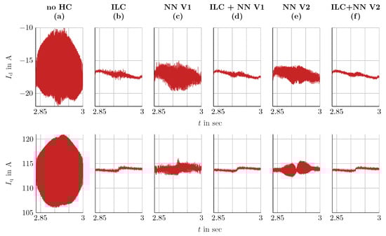
Figure 15.
-currents for the different controllers: variable speed n = 500 rpm to 3000 rpm (see Figure 16), constant torque T = 65 Nm.
Figure 16 shows the speed curve used.
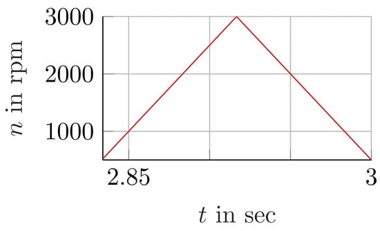
Figure 16.
Speed variation n = 500 rpm to 3000 rpm used for the simulations at variable speed.
5.3. Constant Speed, Variable Torque
The constant speed and variable torque comparison is conducted with the motor operating at a speed of n = 820 rpm. The torque is ramped up from 0 Nm to 150 Nm within 0.1 s and then ramped back down to 0 Nm in the same timeframe. The data presented in Figure 17 and Figure 18 pertain to the 14th ramp, with 13 ramps completed prior to plotting.
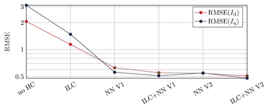
Figure 17.
RMSE calculated from -currents for the different controllers: constant speed n = 820 rpm, variable torque T = 0 Nm to 150 Nm.
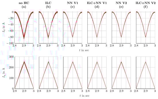
Figure 18.
-currents for the different controllers: constant speed n = 820 rpm, variable torque T = 0 Nm to 150 Nm.
Figure 17 and Table A1 display the RMSE values of the -currents over a duration of 0.2 s. The results indicate that the ILC alone fails to capture the torque variation, while the methods utilizing NNs perform better. The discrepancy between the two NN-based methods is not substantial.
Figure 18 shows the -currents for this operating point. Subplot (a) shows the currents without any harmonic reduction. In contrast, subplot (b) demonstrates that the ILC can mitigate the harmonics to some extent, but the NN-based methods in subplots (c) and (e) offer better performance. Among the methods tested, variant 2 of the NNs combined with the ILC (subplot (f)) performs the best at this operating point.
5.4. Variable Speed, Variable Torque
To conclude, this section gives a comparison at variable speed and variable torque. A speed curve between 500 rpm and 3000 rpm is selected and the torque is specified from the derivative of the speed between −280 Nm and +280 Nm. The variation of speed, torque, and the -currents can be seen in Figure 19.
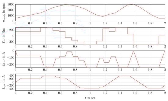
Figure 19.
Speed curve, -currents, and the resulting torque for variable speed n = 500 rpm to 3000 rpm and variable torque T = −280 Nm to 280 Nm.
Figure 19 shows how the specified speed and the torque change for this comparison and which -currents result as the setpoint for the current controller.
Figure 20 illustrates the RMSE for the curve from Figure 19 for the different control variants. The curve here is similar to the previous comparison at constant speed. The ILC can already reduce the RMSE significantly. The NNs can almost halve the RMSE of the ILC, and the combination of NNs and ILC reduces the RMSE even further.
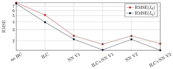
Figure 20.
RMSE calculated from -currents for the different controllers: variable speed n = 500 rpm to 3000 rpm and variable torque to .
6. Conclusions
The simulation results indicate that, depending on the application, combining the ILC with NNs can be advantageous. For constant operating points, the addition of NNs does not make a substantial difference, as the ILC alone can reduce the RMSE for the given operating point by around 98%, while the NNs alone achieve only an 80–85% reduction. In the case of variable speed, the ILC can still reduce the RMSE by approximately 90%, but combining it with NNs yields only a marginal improvement of around 0.5%, while the NNs alone can reduce the RMSE by about 77–80%. When considering variable torque, the ILC alone can only reduce the RMSE by about 48%, while the NNs alone achieve a reduction of about 75–78%. Together, the ILC and NNs can reduce the RMSE by 78–80%, which is approximately 30% more than the ILC alone. The last comparison with variable speed and variable torque shows a similar picture. The ILC reduces the RMSE by 35–50%, the NNs by about 70–73%, and the combination of ILC and NNs can reduce the RMSE by 77–82%.
In conclusion, this paper presents a successful application of ILC and NNs for current harmonic suppression in electric machines. Combining these methods results in improved performance, particularly in the context of varying torque, compared to using ILC alone. To approximate ILC, NNs are utilized directly. The correction signals are decomposed into individual harmonics and the amplitude and phase are then mapped into a separate set of NNs. By decomposing the signal, the size of the NNs required for mapping could be significantly reduced without compromising performance.
The simulations conducted in this study are primarily constrained by the accuracy of the employed model. To conduct a more comprehensive investigation, a more elaborate inverter model is necessary. This enhanced model would include the modeling of switches and their switching behavior. Additionally, the comparisons presented in this study are limited to the base speed range. To evaluate the performance of the proposed method at the modulation limit, appropriate adaptations would need to be made. It would also be valuable to compare the proposed method directly with alternative approaches. The preliminary comparison provided in [] offers an initial indication. By publishing the motor data, the authors also encourage other researchers to perform their own comparisons. Finally, the methods and all the points mentioned must also be tested and validated on the test bench on physical machines. Lastly, it is crucial to test and validate the methods and all the aforementioned aspects on physical machines using a test bench.
Author Contributions
Conceptualization, A.M. and B.W.; funding acquisition, M.H. and B.W.; investigation, A.M. and X.L.; methodology, A.M. and X.L.; resources, M.H. and B.W.; software, A.M.; supervision, B.W. and M.H.; visualization, A.M.; formal analysis, A.M.; writing—original draft preparation, A.M.; writing—review and editing, A.M., B.W., X.L. and M.H.; project administration, B.W. and M.H. All authors have read and agreed to the published version of the manuscript.
Funding
This research was funded by the Federal Ministry for Economic Affairs and Climate Action (19I21030F-KIRA).
Data Availability Statement
The simulation model used in this work is based on data generated by finite element method simulation; flux and torque maps as a function of the -currents and the electrical rotor angle are provided and can be downloaded here: https://doi.org/10.5281/zenodo.7866449.
Conflicts of Interest
The authors declare no conflict of interest.
Abbreviations
The following abbreviations are used in this manuscript:
| ILC | Iterative Learning Control |
| NN | Neural Network |
| PMSM | Permanent Magnet Synchronous Machine |
| VSI | Voltage Source Inverter |
| MPC | Model Predictive Control |
| ML | Machine Learning |
| LUT | Look-Up Tables |
| FOC | Field-Oriented Control |
| MLP | Mulit-Layer Percepton |
| MTPC | Maximum Torque Per Current |
| FFT | Fast Fourier Analysis |
| RMSE | Root Mean Squared Error |
Appendix A. Additional Data
Table A1.
RMSE calculated from -currents for different controllers at different operating conditions.
Table A1.
RMSE calculated from -currents for different controllers at different operating conditions.
| Constant speed n = 820 rpm, constant torque T = 65 Nm | ||
| RMSE() | RMSE() | |
| no HC | 1.7432 | 2.5768 |
| ILC | 0.0330 | 0.0183 |
| NN | 0.4486 | 0.3818 |
| 0.0319 | 0.018 | |
| NN() | 0.3262 | 0.2335 |
| ILC+NN() | 0.0281 | 0.0175 |
| variable speed n = 500 rpm to 3000 rpm, constant torque T = 65 Nm | ||
| no HC | 2.6894 | 4.1972 |
| ILC | 0.3535 | 0.2296 |
| NN | 0.9003 | 0.5234 |
| 0.3406 | 0.2221 | |
| NN() | 0.6470 | 0.5904 |
| ILC+NN() | 0.3337 | 0.2208 |
| Constant speed n = 820 rpm, variable torque T = 0 Nm to 150 Nm | ||
| no HC | 2.0561 | 3.1134 |
| ILC | 1.142 | 1.4802 |
| NN | 0.6275 | 0.5587 |
| 0.5518 | 0.5117 | |
| NN() | 0.5450 | 0.5491 |
| ILC+NN() | 0.5093 | 0.48 |
| variable speed n = 500 rpm to 3000 rpm, variable torque T = −280 Nm to +280 Nm | ||
| no HC | 7.9964 | 7.7304 |
| ILC | 5.1217 | 3.9382 |
| NN | 2.404 | 2.1243 |
| 1.7758 | 1.4426 | |
| NN() | 2.3934 | 2.1151 |
| ILC+NN() | 1.8092 | 1.423 |
References
- Richter, J. Modellbildung, Parameteridentifikation und Regelung Hoch Ausgenutzter Synchronmaschinen. Ph.D. Thesis, Karlsruhe Germany, Karlsruher Institut für Technologie, 2016. [Google Scholar] [CrossRef]
- Wang, X.; Nalakath, S.; Filho, S.; Zhao, G.; Sun, Y.; Wiseman, J.; Emadi, A. A Simple and Effective Compensation Method for Inverter Nonlinearity. In Proceedings of the 2020 IEEE Transportation Electrification Conference Expo (ITEC), Chicago, IL, USA, 23–26 June 2020; pp. 638–643. [Google Scholar] [CrossRef]
- Urasaki, N.; Senjyu, T.; Uezato, K.; Funabashi, T. An adaptive dead-time compensation strategy for voltage source inverter fed motor drives. IEEE Trans. Power Electron. 2005, 20, 1150–1160. [Google Scholar] [CrossRef]
- Lee, J.H.; Sul, S.K. Inverter Nonlinearity Compensation Through Deadtime Effect Estimation. IEEE Trans. Power Electron. 2021, 36, 10684–10694. [Google Scholar] [CrossRef]
- Suriano-Sánchez, S.I.; Ponce-Silva, M.; Olivares-Peregrino, V.H.; De León-Aldaco, S.E. A Review of Torque Ripple Reduction Design Methods for Radial Flux PM Motors. Eng 2022, 3, 646–661. [Google Scholar] [CrossRef]
- Mai, A.; Wagner, B.; Streit, F. Elimination of Current Harmonics in Electrical Machines with Iterative Learning Control. In Proceedings of the 2020 10th International Electric Drives Production Conference (EDPC), Online. 8–9 December 2020; pp. 1–5. [Google Scholar] [CrossRef]
- Zeng, H.; Lorenz, R.D.; van der Broeck, C.H.; De Doncker, R.W. Spatial Repetitive Controller based Harmonic Mitigation Methodology For Wide Varying Base Frequency Range. In Proceedings of the 2019 IEEE Energy Conversion Congress and Exposition (ECCE), Baltimore, MD, USA, 29 September–3 October 2019; pp. 1542–1549. [Google Scholar] [CrossRef]
- Mai, A.; Wagner, B.; Arenz, S. Comparison of Control Algorithms for the Suppression of Current Harmonics in PMSMs. In Proceedings of the PCIM Europe Digital Days 2021; International Exhibition and Conference for Power Electronics, Intelligent Motion, Renewable Energy and Energy Management, Online. 3–7 May 2021; pp. 1–8. [Google Scholar]
- Riaz, S.; Qi, R.; Tutsoy, O.; Iqbal, J. A novel adaptive PD-type iterative learning control of the PMSM servo system with the friction uncertainty in low speeds. PLoS ONE 2023, 18, e0279253. [Google Scholar] [CrossRef] [PubMed]
- Qian, K.; Li, Z.; Chakrabarty, S.; Zhang, Z.; Xie, S.Q. Robust Iterative Learning Control for Pneumatic Muscle With Uncertainties and State Constraints. IEEE Trans. Ind. Electron. 2023, 70, 1802–1810. [Google Scholar] [CrossRef]
- Suh, S.; Kim, W. Position Control Based on Add-on-Type Iterative Learning Control with Nonlinear Controller for Permanent-Magnet Stepper Motors. Appl. Sci. 2021, 11, 587. [Google Scholar] [CrossRef]
- Angalaeswari, S.; Jamuna, K. Design and implementation of a robust iterative learning controller for voltage and frequency stabilization of hybrid microgrids. Comput. Electr. Eng. 2020, 84, 106631. [Google Scholar] [CrossRef]
- Yang, X.; Riaz, S. Accelerated Iterative Learning Control for Linear Discrete Systems with Parametric Perturbation and Measurement Noise. CMES-Comput. Model. Eng. Sci. 2022, 132, 605–626. [Google Scholar] [CrossRef]
- Fei, Q.; Deng, Y.; Li, H.; Liu, J.; Shao, M. Speed Ripple Minimization of Permanent Magnet Synchronous Motor Based on Model Predictive and Iterative Learning Controls. IEEE Access 2019, 7, 31791–31800. [Google Scholar] [CrossRef]
- Bi, G.; Zhang, G.; Wang, G.; Wang, Q.; Hu, Y.; Xu, D. Adaptive Iterative Learning Control-Based Rotor Position Harmonic Error Suppression Method for Sensorless PMSM Drives. IEEE Trans. Ind. Electron. 2022, 69, 10870–10881. [Google Scholar] [CrossRef]
- Basit, B.A.; Rehman, A.U.; Choi, H.H.; Jung, J.W. A Robust Iterative Learning Control Technique to Efficiently Mitigate Disturbances for Three-Phase Standalone Inverters. IEEE Trans. Ind. Electron. 2022, 69, 3233–3244. [Google Scholar] [CrossRef]
- Patan, K.; Patanl, M. Design and convergence of iterative learning control based on neural networks. In Proceedings of the 2018 European Control Conference (ECC), Limassol, Cyprus, 12–15 June 2018; pp. 1–6. [Google Scholar] [CrossRef]
- Zhao, S.; Blaabjerg, F.; Wang, H. An Overview of Artificial Intelligence Applications for Power Electronics. IEEE Trans. Power Electron. 2021, 36, 4633–4658. [Google Scholar] [CrossRef]
- Zhang, S.; Wallscheid, O.; Porrmann, M. Machine Learning for the Control and Monitoring of Electric Machine Drives: Advances and Trends. arXiv 2023, arXiv:2110.05403. [Google Scholar] [CrossRef]
- Bose, B.K. Neural Network Applications in Power Electronics and Motor Drives—An Introduction and Perspective. IEEE Trans. Ind. Electron. 2007, 54, 14–33. [Google Scholar] [CrossRef]
- Bose, B.K. Artificial Intelligence Techniques: How Can it Solve Problems in Power Electronics?: An Advancing Frontier. IEEE Power Electron. Mag. 2020, 7, 19–27. [Google Scholar] [CrossRef]
- Wójcik, A.; Pajchrowski, T. Application of iterative learning control for ripple torque compensation in PMSM drive. Arch. Electr. Eng. 2019, 68, 309–324. [Google Scholar]
- Wang, D.; Chen, Y. Fault-Tolerant Control of Coil Inter-Turn Short-Circuit in Five-Phase Permanent Magnet Synchronous Motor. Energies 2020, 13, 5669. [Google Scholar] [CrossRef]
- Mohammed, S.A.Q.; Nguyen, A.T.; Choi, H.H.; Jung, J.W. Improved Iterative Learning Control Strategy for Surface-Mounted Permanent Magnet Synchronous Motor Drives. IEEE Trans. Ind. Electron. 2020, 67, 10134–10144. [Google Scholar] [CrossRef]
- Pei, G.; Liu, J.; Li, L. Speed Ripple Minimization for PMSM Based on Complex Vector Analysis and Iterative Learning Control. In Proceedings of the 2020 23rd International Conference on Electrical Machines and Systems (ICEMS), Hamamatsu, Japan, 24–27 November 2020; pp. 1442–1447. [Google Scholar] [CrossRef]
- Wu, Z.; Yang, Z.; Ding, K.; He, G. Transfer Mechanism Analysis of Injected Voltage Harmonic and its Effect on Current Harmonic Regulation in FOC PMSM. IEEE Trans. Power Electron. 2022, 37, 820–829. [Google Scholar] [CrossRef]
- Quang, N.P.; Dittrich, J. Praxis der Feldorientieren Drehstromantriebsregelungen; Expert Verlag: Renningen-Malsheim, Germany, 1999. [Google Scholar]
- Kellner, S. Parameteridentifikation bei Permanenterregten Synchronmaschinen. Ph.D. Thesis, Friedrich Alexander Universität Erlangen, Erlangen, Germany, 2012. [Google Scholar]
- Schülting, P.; van der Broeck, C.H.; De Doncker, R.W. A generalized control design approach for a repetitive controller on current harmonics. In Proceedings of the 2015 IEEE 16th Workshop on Control and Modeling for Power Electronics (COMPEL), Vancouve, BC, Cannada, 12–15 July 2015; pp. 1–8. [Google Scholar] [CrossRef]
- Schülting, P.; van der Broeck, C.H.; De Doncker, R.W. Analysis and Design of Repetitive Controllers for Applications in Distorted Distribution Grids. IEEE Trans. Power Electron. 2019, 34, 996–1004. [Google Scholar] [CrossRef]
- Wagner, B. Analytische und Iterative Verfahren zur Inversion Linearer und Nichtlinearer Abtastsysteme. Ph.D. Thesis, Friedrich Alexander Universität Erlangen, Erlangen, Germany, 1998. [Google Scholar]
Disclaimer/Publisher’s Note: The statements, opinions and data contained in all publications are solely those of the individual author(s) and contributor(s) and not of MDPI and/or the editor(s). MDPI and/or the editor(s) disclaim responsibility for any injury to people or property resulting from any ideas, methods, instructions or products referred to in the content. |
© 2023 by the authors. Licensee MDPI, Basel, Switzerland. This article is an open access article distributed under the terms and conditions of the Creative Commons Attribution (CC BY) license (https://creativecommons.org/licenses/by/4.0/).