Abstract
In this paper, the direct differentiation of generalized- time integration is derived, equations are introduced and results are shown. Although generalized- time integration has found usage, the derivation and the resulting equations for the analytical sensitivity analysis via direct differentiation are missing. Thus, here, the sensitivity equations of generalized- time integration via direct differentiation are provided. Results with generalized- are compared with Newmark- time integration and their sensitivities with numerical sensitivities via forward finite differencing in terms of accuracy and performance. An example is shown for each linear structural dynamics and flexible multibody dynamics.
1. Introduction
Analytical design sensitivity analysis is developed in this paper for the generalized-α family of time integration. After deriving and introducing design sensitivity using direct differentiation, results are compared with numerical differentiation via forward differencing in terms of accuracy and computational effort.
Efficient sensitivity analysis is the centerpiece of efficient and effective gradient-based design optimization. Other uses of sensitivity analysis include uncertainty analysis and quantification, e.g., the adjoint variable method applied to the sensitivity analysis with respect to uncertain and random variables was developed in [1]. Overviews of design sensitivity analysis are provided by [2,3,4,5,6]. In transient problems, sensitivity analysis must be extended to time integration [7,8], which is handled here by introducing and deriving the equations for the direct differentiation of the generalized-α family of time integration.
In the dynamic systems addressed, the transient response (response in time domain) is of interest and therefore a temporal discretization is applied. The calculation of the system responses, here position, velocity and acceleration, can be carried out with explicit or implicit time integration methods. Implicit time integration allows for larger time steps than explicit methods, which is bounded by the Courant criterion to remain stable [9].
Newmark introduced an implicit integration scheme, now referred to as Newmark-β, in 1959 with two integration parameters and [10]. The Hilber–Hughes–Taylor (HHT) method was introduced in 1977 to improve upon Newmark with the additional integration parameter for numerical damping [11], while the Wood–Bossak–Zienkiewicz (WBZ, also known as simply Bossak or Wood) introduced the parameter [12]. Generalized-α was introduced by Chung and Hulbert in 1993 [13] to generalize all these methods with the integration parameters , , and . These methods can be generalized via a single implementation which is therefore referred to as the generalized-α family of time integrators. In the generalized-α method, for which the family is named, all parameters can be controlled by a single value, namely the spectral radius at infinity ranging from zero, being the highest amount of damping, to unity, being none [13]. It should be noted that we differentiate between the variants of the Greek letter rho: is used here for the spectral radius at infinity, while is used below for density. The mapping of to , , and is shown below. The choice of this value can affect the response for a given time step, see, e.g., [14].
Generalized-α time integration has found usage in both nonlinear structural dynamics and multibody dynamics. Multibody dynamics addresses the dynamic response with kinematic constraints. Rigid multibody dynamics considers the bodies rigid, while flexible multibody dynamics allows for the deformation in the bodies of the system. Applications are shown including both linear structural dynamics and flexible multibody dynamics.
This paper is concerned with the sensitivity analysis of dynamic problems, which is used when one or more parameters affect the system responses. The calculation of the system responses is referred to here as primal analysis so that it may be distinguished from the sensitivity analysis. This is of interest for the efficient design optimization via gradient-based optimization algorithms in addition to investigating the sensitivities themselves or for uncertainty analyses. Methods for sensitivity analysis include analytical, numerical, complex step and algorithmic approaches [5].
Analytical sensitivities can be derived either manually (by hand) or via the automatic differentiation [15,16] of the implemented code. The automatic differentiation and manual differentiation of rigid multibody systems are compared in [17]. Although prone to human error and not automatic, the former represents an exact and one of the fastest methods for sensitivity analysis [18]. Manual sensitivity analysis requires high implementation effort, but the resulting code is typically highly reusable and must therefore only be derived and implemented once. Due to its physics- and knowledge-based nature, in addition to its increased transparency, hand differentiation is preferred by the authors.
This study limits itself to analytical sensitivity analysis, which is further divided into direct differentiation (also known as forward sensitivity analysis) and the adjoint variable method (also known as backward sensitivity analysis). Generally, it can be said that direct differentiation is more efficient than the adjoint variable method if the number of design variables is less than the number of functions to differentiate, i.e., in optimization, the sum of the number of objective functions (one in case of single objective optimization) and the number of constraints. Due to its nature, the adjoint variable method must be performed after the time integration of the primal analysis and integrated backwards in time. Thus, the adjoint variable method, in contrast to direct differentiation, needs dedicated solver routines to integrate backwards in time and cannot reuse primal forward time integration [7,8]. Furthermore, for nonlinear analysis, the system matrices must be stored or recalculated when integrating backwards in time. Therefore, direct differentiation is chosen in this work. The reader is referred to the following literature for the adjoint variable method: [19,20,21,22,23,24,25,26,27,28,29,30].
A number of studies have been carried out for sensitivity analysis in transient structural dynamics and multibody dynamics. Early works on sensitivity analysis with transient structural dynamics include [31], which bridges sensitivities in static and dynamic analysis via the adjoint variable method, including maximum-value objectives and constraints. In [32], sensitivity analysis with the adjoint variable method and direct differentiation is introduced for time-averaged and time-specific constraints. The German-language monograph [33] clearly demonstrates the analytic sensitivity analysis of transient linear dynamics with Newmark-β time integration, providing all necessary equations for implementation, which also includes the sensitivity of the duration of a dynamic operation. The adjoint variable method for transient structural dynamics with Newmark-β time integration is derived by [34]. The adjoint variable method and direct differentiation of nonlinear and transient problems is handled by [35] in which the crucial aspects of the nonlinear solver for sensitivity analysis are introduced.
The sensitivity analysis of multibody systems is often limited to the governing equations and often not extended to the nonlinear solver or time integration. Exceptions to this can be found for direct differentiation with the divide-and-conquer-based modal superposition method in [36]; for direct differentiation and the adjoint variable method with general formulations of differential–algebraic equations in [37]; for direct differentiation and the adjoint variable method of ordered differential equations in [38]; and for the adjoint variable method with the floating frame of reference formulation in [20]. The adjoint variable method of the governing equations in descriptor form and for generic optimization functions is shown by [21] for several time integration methods, including the backward difference formula, Newmark-, Adams–Bashforth–Moulton and diagonally implicit Runge–Kutta. The derivation of the adjoint variable method based on generalized-α time integration and applied to the finite-element-based formulation is provided by [39]. The transient response sensitivity analysis of localized nonlinear behavior using Newmark-β [40].
Higher-order sensitivities can also be of interest, especially in cases of a low number of degrees of freedom and design variables. Second-order sensitivities via the adjoint variable method with the Runge–Kutta–Fehlberg method are shown in [41]. Second-order sensitivities for multibody systems with the adjoint variable method and differential–algebraic equations are shown in [42]. Higher-order sensitivities are used in [43,44] to develop a surrogate model for optimization. This work is limited to first-order sensitivities, as required by gradient-based optimization, although the equations provided can be readily extended to higher-order derivatives.
The scope here is thus the investigation of the direct differentiation of the generalized-α method. A method in this regard is introduced in [45], yet the needed equations are not derived and shown. The present work builds upon and extends the works to generalized-α. The authors developed Newmark-β sensitivities in [7,46], which are in turn based on [33,34]. In this paper, Newmark-β serves as a comparison to the developed method for generalized-α.
This work first generally introduces generalized-α time integration and its equations. Afterwards, the sensitivity equations are introduced for structural dynamics and flexible multibody dynamics, respectively. A numerical example is shown for each and the results are provided for both the primal and sensitivity analyses in comparison with Newmark-β time integration. We close with a conclusion, including a discussion of this work. Furthermore, a detailed derivation of the effective system matrices is provided in the Appendix A and Appendix B.
2. Sensitivity Analysis with Generalized-α Time Integration
In this section, we introduce the equations for an acceleration-form (a-form) of generalized-α time integration using a predictor–corrector scheme and extend this for sensitivity analysis. The acceleration-form refers to the formulation, where the acceleration is the primary variable (i.e., the variable for which it is being solved), and contrasts with the displacement-form (d-form) in which the displacement is the primary variable. The predictor–corrector scheme allows for nonlinear terms in the governing equation in which the predicted values are updated in the nonlinear solver, e.g., Newton–Raphson, and then corrected.
In this work, we extend the well-established generalized-α time integration method to include design sensitivity analysis, which is defined by the differentiation with respect to the design variables (but could include other parameters, e.g., uncertain parameters). Sensitivity analysis is carried out here by directly differentiating both the equations of the time integration as well as the governing equations. We consider both linear structural dynamics as well as flexible multibody dynamics, which is intrinsically nonlinear. After introducing the general equations for generalized-α time integration and its sensitivities, the domain-specific governing equations for linear structural dynamics and flexible multibody dynamics are given. Flexible multibody dynamics is shown using the specific approach developed in [7,47,48] with an index-1 approach and the floating frame of reference formulation.
2.1. Generalized- Time Integration
The method for primal and sensitivity analysis with generalized-α time integration is introduced in the following. This is based on Newmark’s equations for the updated position and velocity vectors with the calculated value of the acceleration vector ,
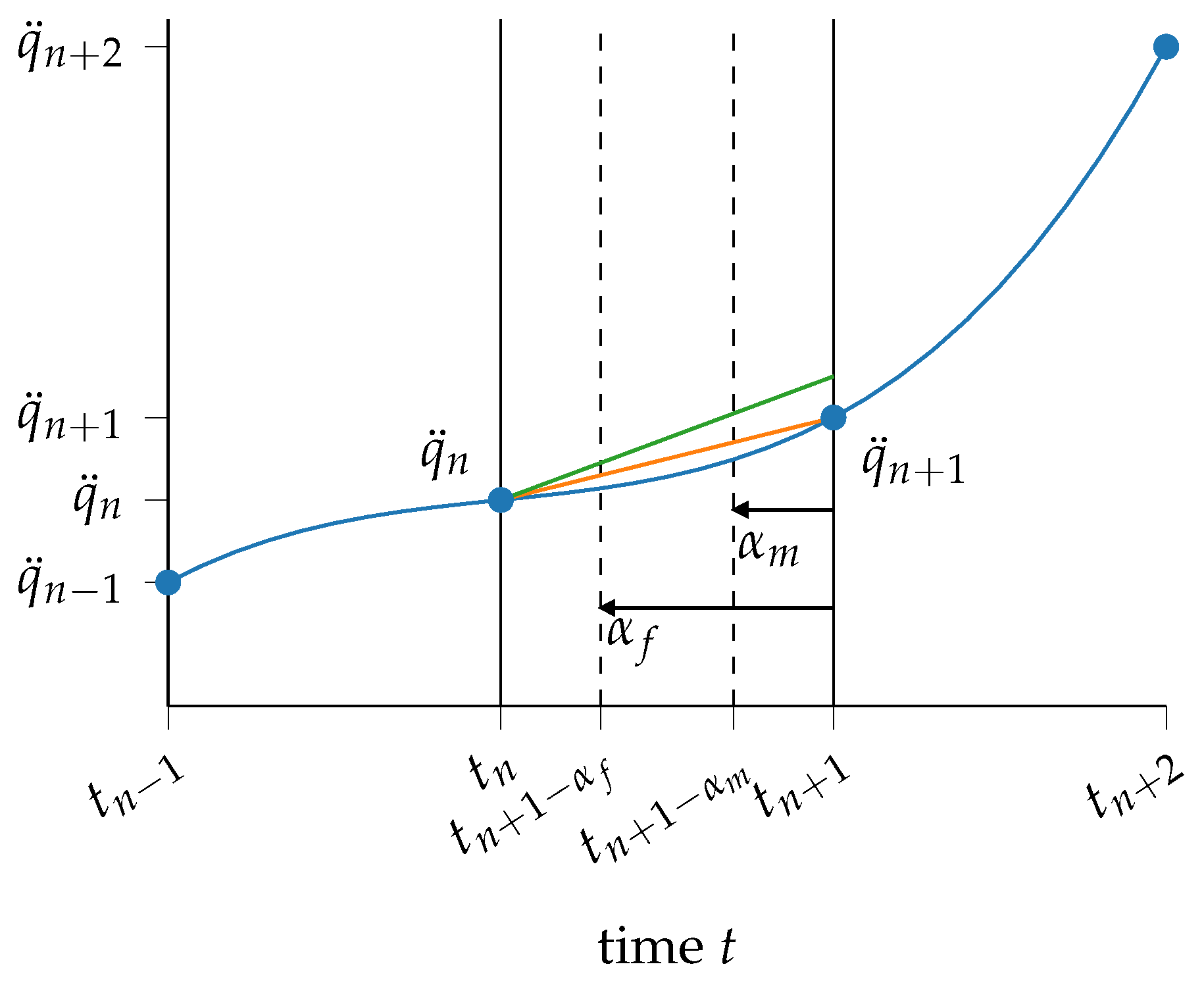
where and are the Newmark integration parameters. Though the simulation is evaluated at the times and , values at intermediate points are interpolated. The position q and velocity use time and the acceleration uses time , giving the approximations by linear interpolation (see Figure 1),
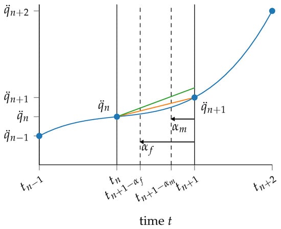
Figure 1.
Time integration with — acceleration, — , — .
Figure 1.
Time integration with — acceleration, — , — .
For the sensitivity analysis within the generalized-α time integration, we use the direct differentiation of the approximations
where the nabla operator ∇ denotes the design sensitivity, i.e., the total derivative with respect to the design variables, e.g., for the sensitivity scalar response with respect to the design variable vector,
The same direct differentiation is applied to the predictors, which are then defined by
After calculating by use of the effective sensitivity system (see below for explanation of structural dynamics and flexible multibody dynamics, respectively), the following correctors are used:
For a nonlinear analysis, a Newton solver can be integrated into the solving routine. This is explained with flexible multibody systems below in Section 2.3.
The time integration constants of generalized-α are , , and and their choice can lead to a number of established time integration methods, including the Newmark family of integrators, Hilber–Hughes–Taylor and Wood–Bossak–Zienkiewicz. Therefore, this can then be referred to as the α-family of time integrators. The equations introduced above in this section can therefore be generally used within this family. Specifically for the generalized-α time integration used here, the choice of integration constants can be tied to a single user-defined parameter, and the spectral radius at infinity [13],
The spectral radius at infinity is sometimes referred to as the (numerical) damping and is limited to a range of . The value returns the Newmark-β retaining frequencies, which are preserved, while annihilates all frequencies above after one time step in which T is the period of the highest frequency of interest. The results converge to those without numerical damping when the time step goes to zero. Thus, the level of numerical damping introduced to generalized-α time integration depends on both the step size as well as the spectral radius at infinity and the choice is critical for proper results. A parameter study with a fixed-time step and varying the values of the spectral radius at infinity is shown in [14]. As the present study develops a general framework for this methodology, this is not addressed here and the reader is referred to [13,49,50,51]. In this paper, we use a moderate value of , though the sensitivity analysis methodology developed is general and independent of this parameter value.
2.2. Structural Dynamics
The governing equation for linear structural dynamics is defined by the following second-order equation of motion:
where is the mass matrix, is the damping matrix, is the stiffness matrix and is the external force vector. For linear structural dynamics, the system matrices are constant and independent of position and time. For the solving scheme, we add the residual force vector , which is to be zero (to an allowable value) at all times, to the right-hand side. The α-family of integration methods uses intermediate-point approximations between and , namely and , revealing
where the linear approximation of the intermediate external force is
The effective equation of motion is defined by
where
For the derivation of the effective mass matrix and effective force vector for generalized-α method, see Appendix A.1.
The sensitivity analysis is derived using the direct differentiation which is applied to the governing Equation (23). This reveals the sensitivity of the force balance for the α-family of integration methods as
where the intermediate external force sensitivity is found with the approximation
The design sensitivities of the system matrices are three-dimensional matrices and therefore efficient handling is needed.
The effective equation of motion for sensitivities is defined by the differentiation of (25),
where
and fully expressed by
For the derivation of the effective mass matrix and effective pseudo force for the generalized-α method, see Appendix A.1 and Appendix A.2.
2.3. Flexible Multibody Dynamics
Flexible multibody dynamics is the analysis of mechanical systems consisting of flexible bodies constrained by kinematic joints modeled with differential–algebraic equations. This work builds upon the previous work of analytical sensitivity analysis with multibody dynamics, including [37,52,53]. In addition to the kinematic constraints with respect to structural dynamics, multibody dynamics also must integrate a nonlinear solver in order to consider the dependencies of the system matrices and vectors on the state variables. This is carried out with Newton steps.
The flexible multibody system is modeled with the floating frame of the reference formulation [54,55,56]. The generic index-3 differential–algebraic equation for a flexible multibody system with holonomic constraints is written as follows:
where , and are the generalized position, velocity and acceleration vectors; is the vector of Lagrange multipliers of kinematic constraints; the matrices , , and are the mass, damping and stiffness matrices; is the Jacobian matrix of kinematic constraints; is the vector of external forces; is the quadratic velocity vector; and is the vector of kinematic constraints at the position level.
Numerical problems related to the solution of index-3 differential–algebraic equations [57] can be avoided by a number of methods including index reduction, coordinate reduction, augmented Lagrangian formulation and preconditioning [58,59,60]. Although generalized-α time integration is suitable for directly solving index-3 or index-2 differential–algebraic equations, in this work, we address the problem using index reduction leading to an index-1 differential–algebraic equation in which the kinematic constraint function is differentiated twice with respect to time,
where is the right-hand side of acceleration constraints. As index-1 differential–algebraic equations are susceptible to drift in the kinematic constraints, Baumgarte stabilization [61] is used. Kinematic constraint drift is stabilized in this method by adding damping and restoring terms to the acceleration constraint equations that are proportional to the velocity and position constraints. Details of its implementation, including the sensitivity analysis, are described in [14,62].
The generalized-α time integration is based on
with the intermediate approximations of all force terms of the equations of motion. These intermediate approximations are shown in Appendix B.1. Inserting the intermediate approximations of the force terms acting on the flexible multibody system leads to the equations of motion in residual form given by
In the case of a nonlinear mass matrix, as is the case with the floating frame of reference formulation, this weighted formulation of the residual equations are first-order accurate. For a formulation of second-order accuracy, see, e.g., [63], where the dynamic equilibrium is enforced exactly at the time steps of the simulation. The derived time integration and its differentiation with the weighted residual formulation can be extended and applied to further formulations.
The effective equation of motion is defined by
where
The derivations of the effective equation of motion and the terms , , and are shown in Appendix B.1.
With flexible multibody dynamics, the system parameters (matrix- and vector-valued for ) including mass, damping, stiffness, constraints and forces are generally dependent on state variables. Therefore, a nonlinear solver is needed to solve the system and the Newton–Raphson method is used here of the following form:
With the dependencies shown in (33) and (34), and the terms of the Jacobian matrix (tangent operator) of the residuals with respect to and are given by
The derivation of these terms is shown in Appendix B.2.
The direct differentiation of the equations of motion (39) and (40) leads to the governing equation of the sensitivity analysis,
The governing sensitivity equation of the effective system is defined by the differentiation of (41),
where
leading to
The derivation of the effective mass matrix and the effective constraint Jacobian matrix is shown in Appendix B.1 and the derivation of the effective pseudo force terms is shown in Appendix B.3.
The Newton–Raphson step for the sensitivity analysis is given by
As shown in [7], the Jacobian of the residual sensitivity with respect to and reduces to
which reduces the dimensions of the coefficient matrix from to . The solution of the resulting equation,
is found using the same solving scheme for the nonlinear solver of the primal analysis (46). Furthermore, both the primal analysis (46) and sensitivity analysis (59) have the same coefficient matrix, which also allows one to reuse the coefficient matrix of the primal analysis in the sensitivity analysis without the need for further evaluations.
3. Numerical Results
In this section, numerical results are shown comparing the introduced method for the sensitivity analysis for generalized-α time integration (primal analysis introduced in Section 2) with that of Newmark-β. The methods are compared with applications to both structural dynamics as well as flexible multibody dynamics.
3.1. Structural Dynamics
The linear structural dynamic problem used here as a demonstration example is based on [64], which has found usage as a benchmark in [65,66,67,68,69,70,71]. This unitless problem is schematically shown in Figure 2. This problem is defined by
with the prescribed displacement,
and the unitless values

Figure 2.
Structural dynamics example.
The masses and as well as the stiffnesses and are considered design variables with respect to which the design sensitivities are calculated. The problem consists of stiff ( and flexible ( parts that are typical of complex, practical structural–mechanical systems [64].
Considering the prescribed displacement, this problem can be reduced to two degrees of freedom,
which we implement in our in-house, Python-based solver framework SiMuLi in the time with the initial conditions
As reported in [64], unitless time steps of are used, giving the following values for the ratio step size to the fundamental periods of the system:
where is the fundamental period of the forcing function and , for the first and second modes, and .
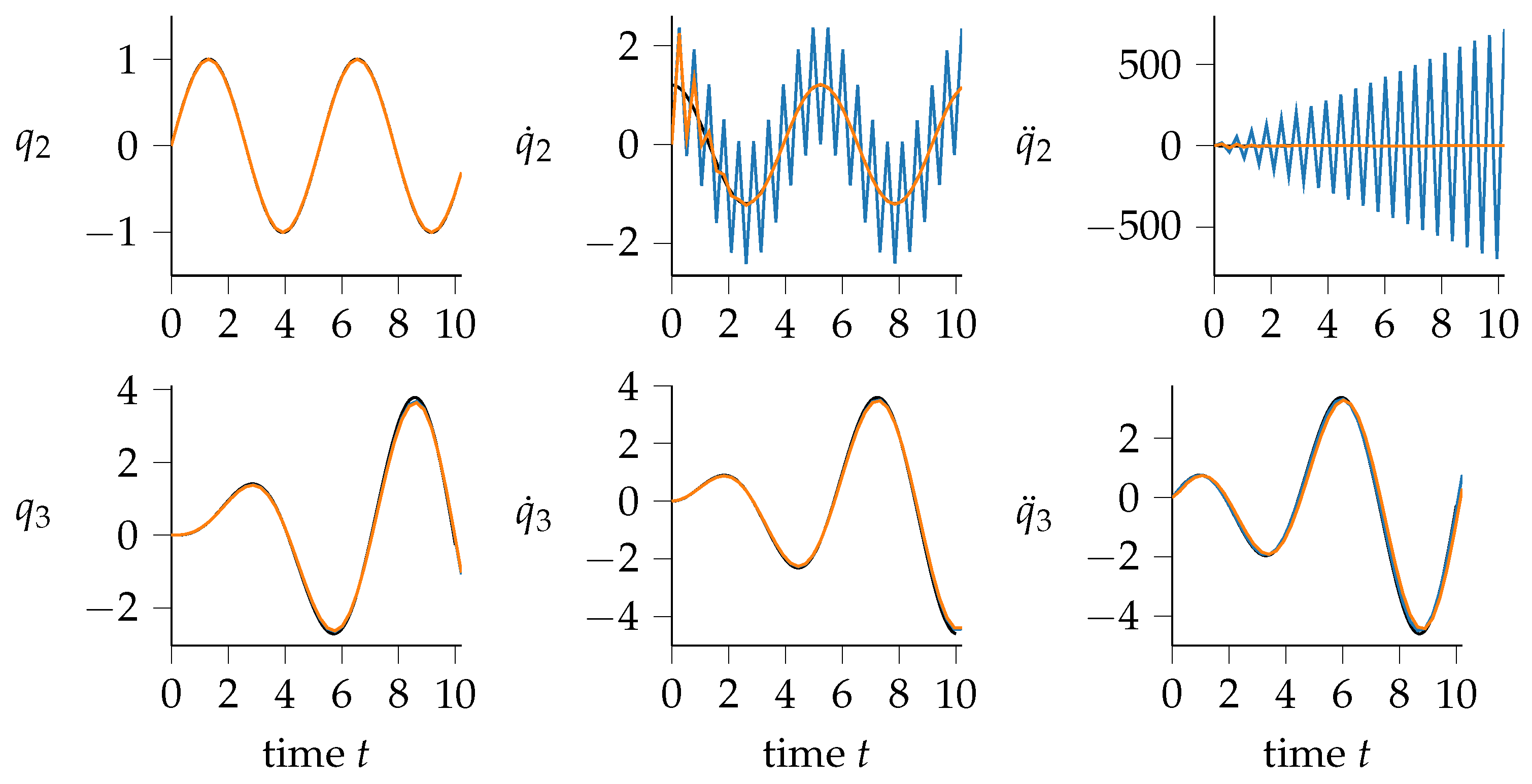
The results for both Newmark-β and generalized-α time integration methods are shown in Figure 3 and compared with the exact solution. The exact solution is calculated via mode superposition per [72]. The numerical damping parameter of generalized-α time integration is set as . As expected with generalized-α time integration, the unphysical, high-frequent oscillatory behavior of the response can be avoided. As such, the beneficial effects of numerical damping with generalized-α time integration can be clearly seen in the velocity and acceleration of node 2, while maintaining the integrity of the other responses.
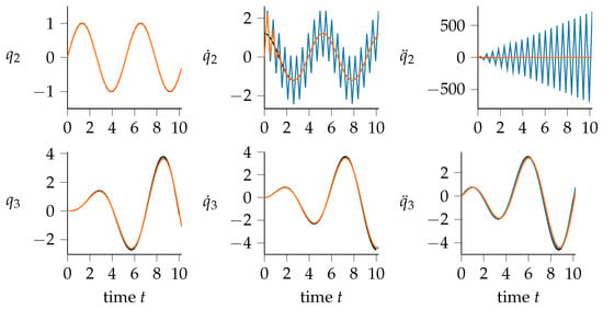
Figure 3.
Responses of the structural dynamic example (unitless) calculated with —Newmark-β and —generalized-α compared with — exact solution (undermost line).
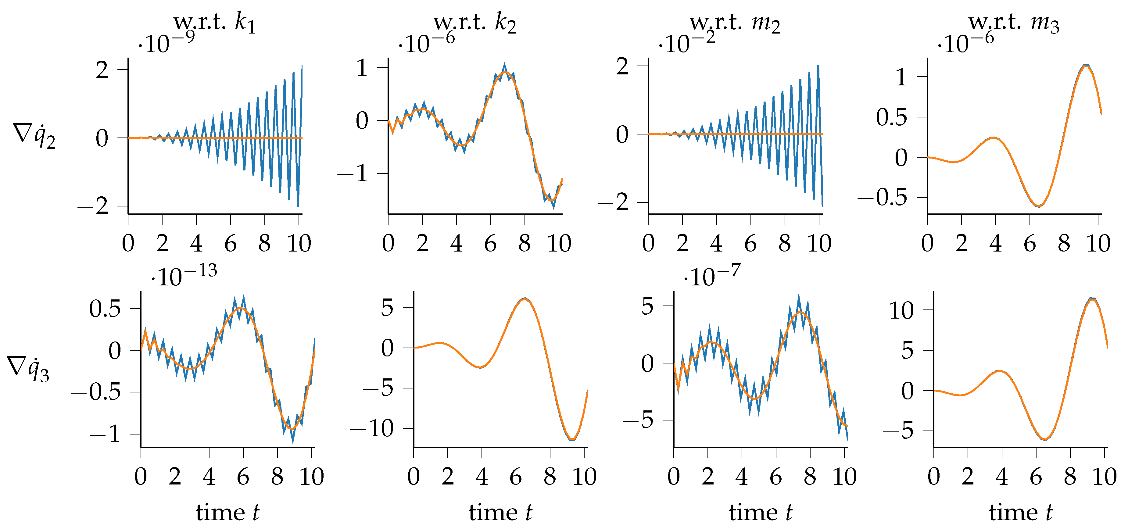
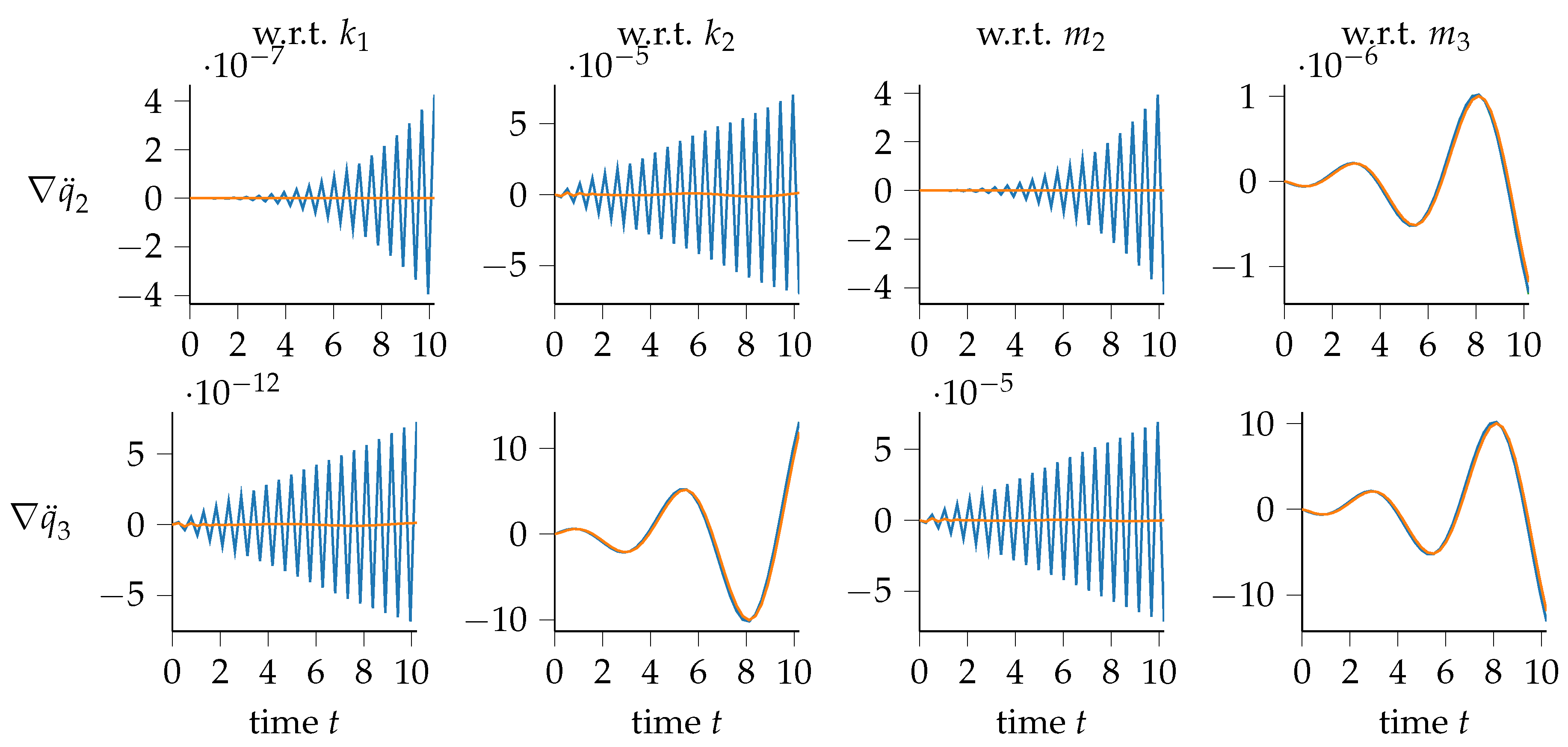
The sensitivity analysis developed above is applied and these results can be seen in Figure 4, Figure 5 and Figure 6. Analytical sensitivity analysis with Newmark-β and generalized-α time integration methods are also compared with their numerical sensitivity implementations via finite differencing using a relative perturbation of .
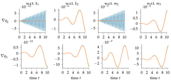
Figure 4.
Position sensitivities of the structural dynamic example with respect to , , and (unitless), analytically calculated with —Newmark-β and —generalized-α compared with those calculated numerically via finite differencing with —Newmark-β and —generalized-α (undermost lines). Note: no visible difference between finite differencing and analytical sensitivities.
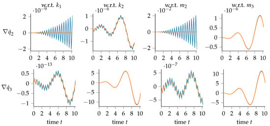
Figure 5.
Velocity sensitivities of the structural dynamic example with respect to , , and (unitless), analytically calculated with —Newmark-β and —generalized-α compared with those calculated numerically via finite differencing with —Newmark-β and —generalized-α (undermost lines). Note: no visible difference between finite differencing and analytical sensitivities.
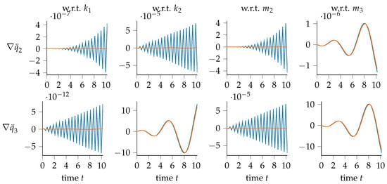
Figure 6.
Acceleration sensitivities of the structural dynamic example with respect to , , and (unitless) analytically calculated with —Newmark-β and —generalized-α compared with those numerically calculated via finite differencing with —Newmark-β and —generalized-α (undermost lines). Note: no visible difference between finite differencing and analytical sensitivities.
In cases where the Newmark-β time integration shows instability or noise, the numerical damping allows for usable sensitivities. In some cases, noise—albeit at a much lower level—persists in the first iterations before being damped out—after approximately (or approximately 10 iterations). Attention is drawn to those sensitivities susceptible to stability issues, namely
- sensitivities of position 2 with respect to stiffness 1 and mass 2 (Figure 4);
- sensitivities of velocity 2 with respect to stiffness 1 and mass 2 (Figure 5);
- sensitivities of acceleration 2 with respect to stiffness 1, stiffness 2 and mass 2 (Figure 6);
- sensitivities of acceleration 3 with respect to stiffness 1 and mass 2 (Figure 6).
Generalized-α time integration is not afflicted by this instability, resulting in sensitivities that can be successfully used in gradient-based algorithms.
Furthermore, generalized-α time integration eliminates the noise in those sensitivities present when using Newmark-β. This is seen with the following sensitivity responses:
The analytical and numerical results are, in most plots, nearly exact. There are cases, however, where the negative consequences of the numerical instability with Newmark-β are increased. The reader’s attention is especially called to
- sensitivity of velocity 2 with respect to stiffness 2 (Figure 5);
- sensitivity of velocity 2 with respect to mass 3 (Figure 5);
- sensitivity of acceleration 2 with respect to stiffness 2 (Figure 6);
- sensitivity of acceleration 2 with respect to mass 3 (Figure 6).
It can be seen that both analytical and numerical sensitivities with generalized-α time integration are not negatively affected by numerical instabilities, as is the case with Newmark-β.
The number of time steps needed for the damping to take effect can be reduced by reducing the numerical damping parameter towards zero (i.e., more damping), though also affecting the physical response to a greater degree. As time continues, the instability grows, with Newmark-β time integration and therefore a clear advantage can be seen with generalized-α. It can be clearly seen how gradient-based solvers would struggle to use the gradient information provided with Newmark-β time integration.
For our modest case of four design variables, we show an acceleration of two, where the speedup S is defined by the ratio of computational time for finite differencing to that of analytical sensitivities ,
The computational time required for analytical sensitivity analysis represents approximately the ideal computational effort twice that of the primal analysis, i.e., analysis without sensitivity analysis. Computation reduction is the same for both Newmark-β and generalized-α time integration methods, as can be seen in Table 1.

Table 1.
Computational effort for the structural dynamics example.
3.2. Flexible Slider–Crank Mechanism
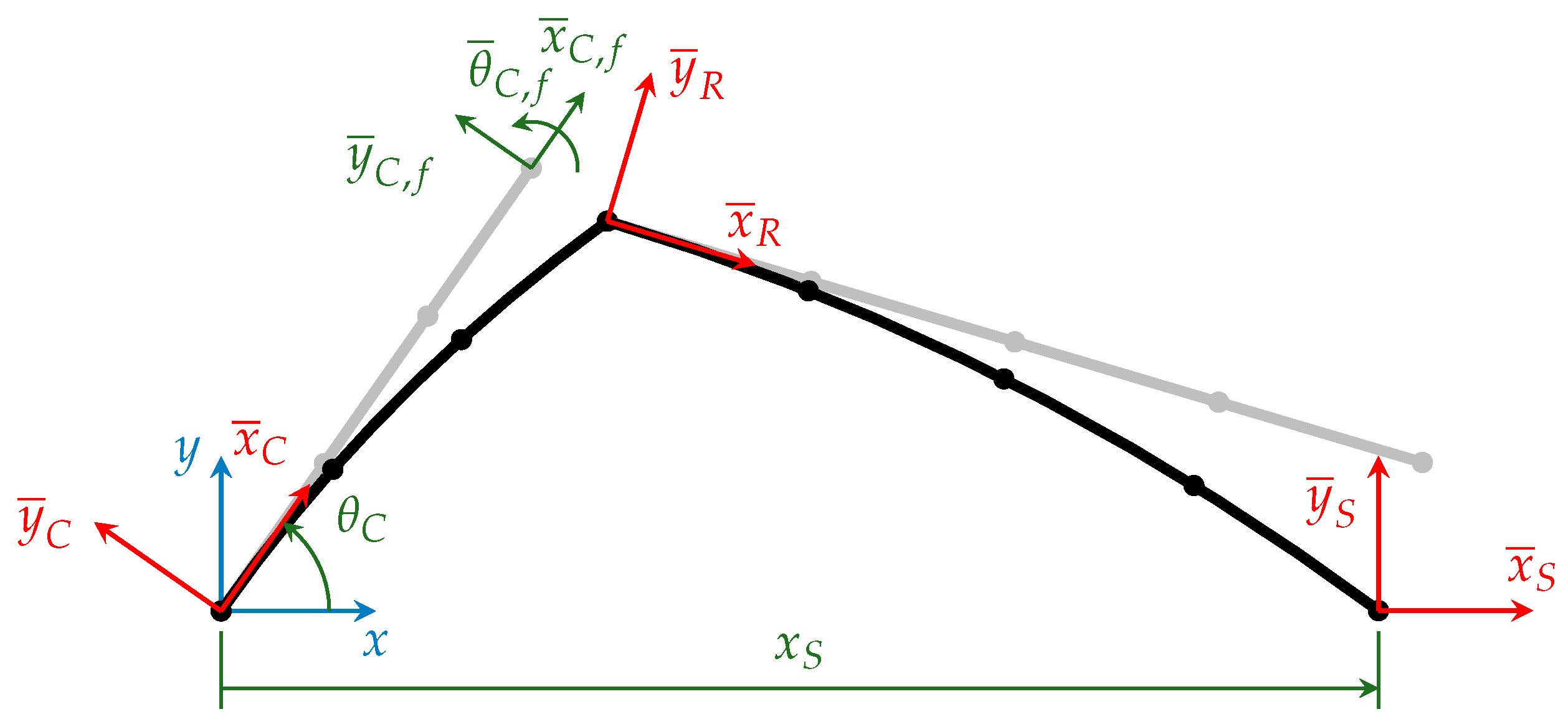
The slider–crank mechanism, as shown in Figure 7, is modeled with flexible multibody dynamics using the floating frame of reference formulation. The mechanism consists of four bodies that are connected by three revolute joints and one prismatic joint, modeled as ideal joints without friction. The ground and the slider are considered to be rigid, while the crank and the rod are considered to be flexible and are modeled with Euler–Bernoulli beams. Figure 8 shows the flexible multibody system of the mechanism. The inertial reference frame coinciding with the reference frame of the ground is shown in blue. The body reference frames of the crank, the rod and the slider are shown in red. The undeformed bodies of the crank and the rod are shown in gray and the deformed bodies are shown in black, where the points represent the nodes of the finite elements for the geometric discretization. The coordinates that are investigated in detail for the primal analysis and the sensitivity analysis are shown in green. The dimensions of the bodies are listed in Table 2. The bodies are made of steel and Table 3 shows the material properties. A linear elastic material model with isotropic behavior is applied. In this example, the SI-derived MPa unit system is used with length in millimeters (mm), mass in tonnes (t), time in second (s), force in Newtons (N), Angle in radian (rad) and stress in megapascals (MPa).
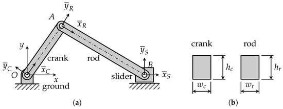
Figure 7.
Slider–crank mechanism: (a) schematic diagram; and (b) cross-sections.
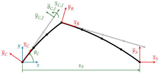
Figure 8.
Flexible multibody system of the slider–crank mechanism with the undeformed bodies in gray, the deformed bodies in black, the inertial reference frame in blue, the body reference frames in red and the coordinates that are investigated in green.

Table 2.
Geometry of the slider–crank mechanism.

Table 3.
Material properties.
The generalized coordinates of a flexible multibody system modeled with the floating frame of the reference formulation and Euler–Bernoulli beams are given by
where is the position of the body reference frame, is the orientation of the body reference frame and are the nodal displacements in the body coordinates of each node on the flexible body. Since no damping is considered, the equations of motion of a flexible body are given by
where the system matrices of the flexible bodies are given by
and the system vectors are given by
with the index denoting translational terms t, rotational terms r and flexible terms f.
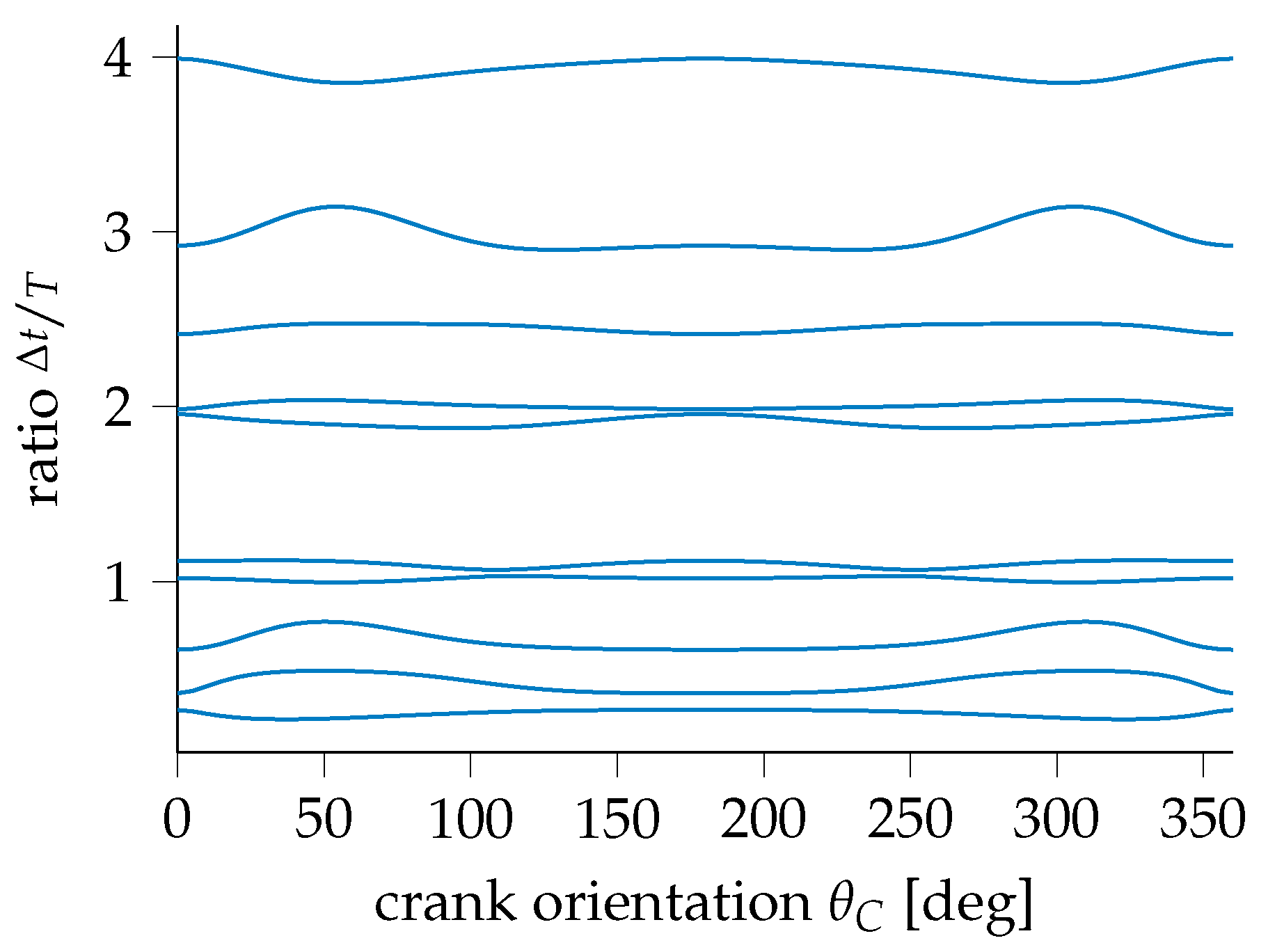
For the dynamic simulation of the mechanism, the above-mentioned solver framework SiMuLi is used. The simulation is performed in the time interval . For both generalized-α and Newmark-β time integration, a time step of is chosen for comparison. The resulting values for the ratio step size to fundamental periods of the system for the first ten non-zero eigenfrequencies are found in Figure 9. The values for the ratio step size to fundamental periods range from for first non-zero eigenfrequency to for the tenth non-zero eigenfrequency and to for the twentieth non-zero eigenfrequency (not pictured in the plot).
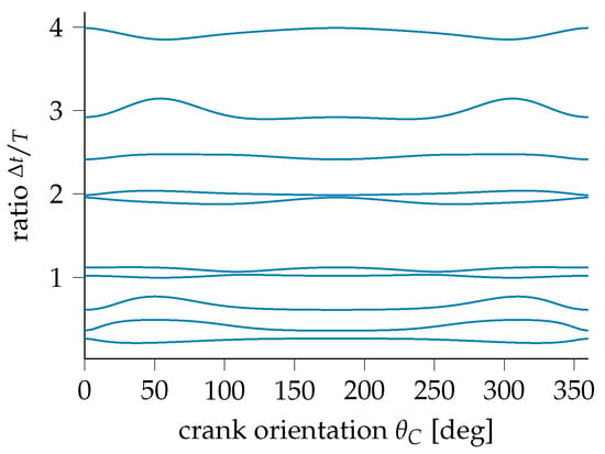
Figure 9.
Ratio time step to fundamental periods for the first ten non-zero eigenfrequencies of the slider–crank mechanism.
For the initial conditions, the angular position and velocity of the crank are defined with
and the initial conditions of the other bodies are derived through the kinematic analysis of the system. The dimensions of the cross-sections of the crank , and the rod , are used as design variables in the sensitivity analysis.
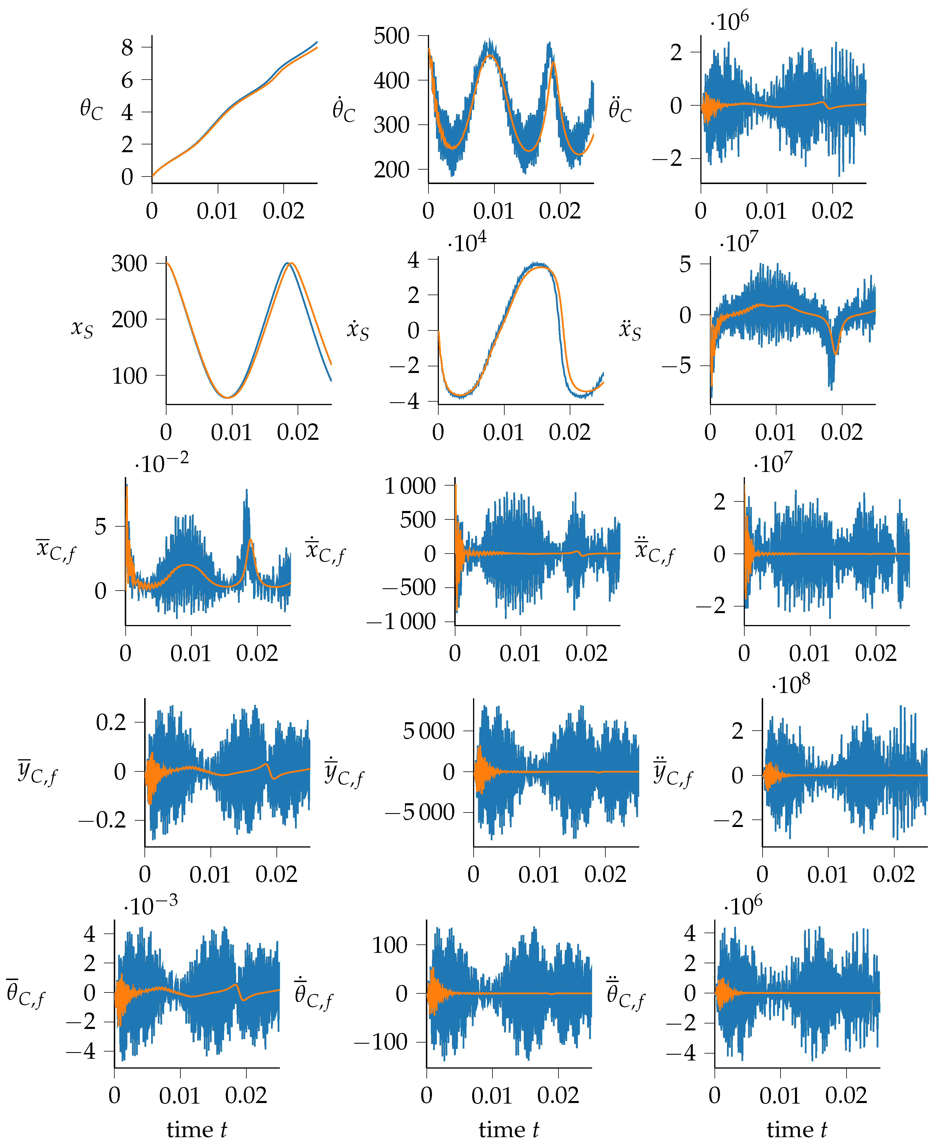
The results of the simulation of the coordinates that are highlighted in Figure 8 are shown in Figure 10. With Newmark-β, vibrations at high frequencies are observed. With generalized-α, vibrations are observed in the beginning of the simulation that are numerically damped with ongoing simulation time. In addition to the generalized coordinates, the maximum stresses on the upper and lower fiber of the beam elements of the flexible bodies including the crank and the rod are computed. The Kreisselmeier–Steinhauser function [73,74] is used to approximate the maximum stress value of the bodies at each time step with a differentiable function and the results are shown in Figure 11. With Newmark-β, the vibrating behavior of the system causes higher flexible deformation and therefore unrealistic high stress in the components. The numerical damping with generalized-α leads to lower maximum stress values and a more realistic stress distribution over time.
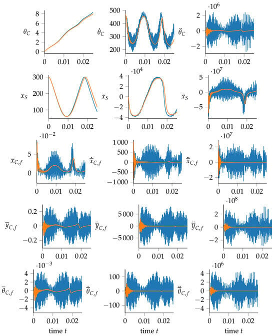
Figure 10.
Responses of the slider–crank mechanism (values in MPa units, i.e., s, mm, , for translations and rad, , for rotations) calculated with —Newmark-β and —generalized-α.

Figure 11.
Maximum stress in MPa on the upper and lower fiber of the crank and the rod over time in s calculated with —Newmark-β and —generalized-α.
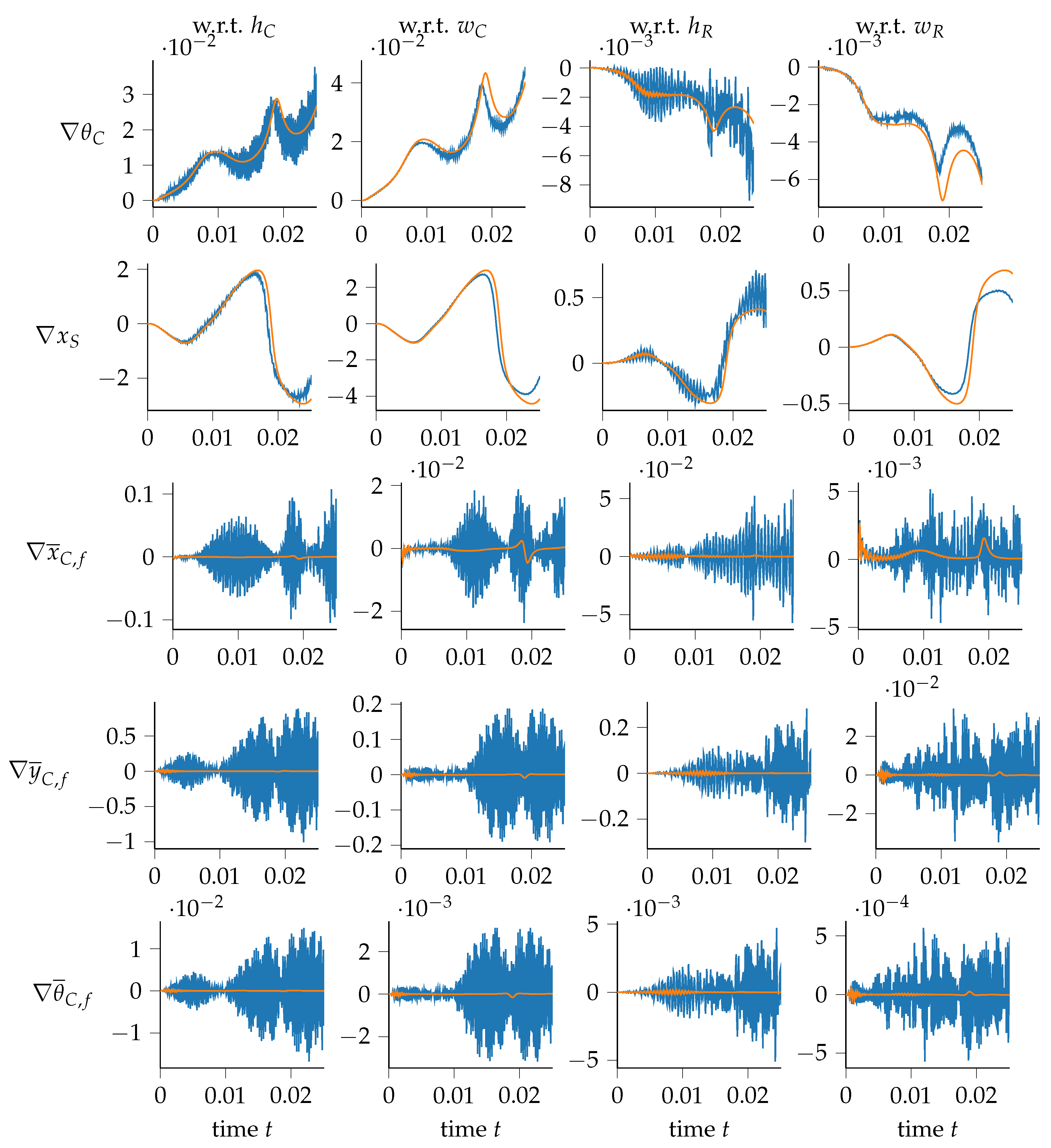
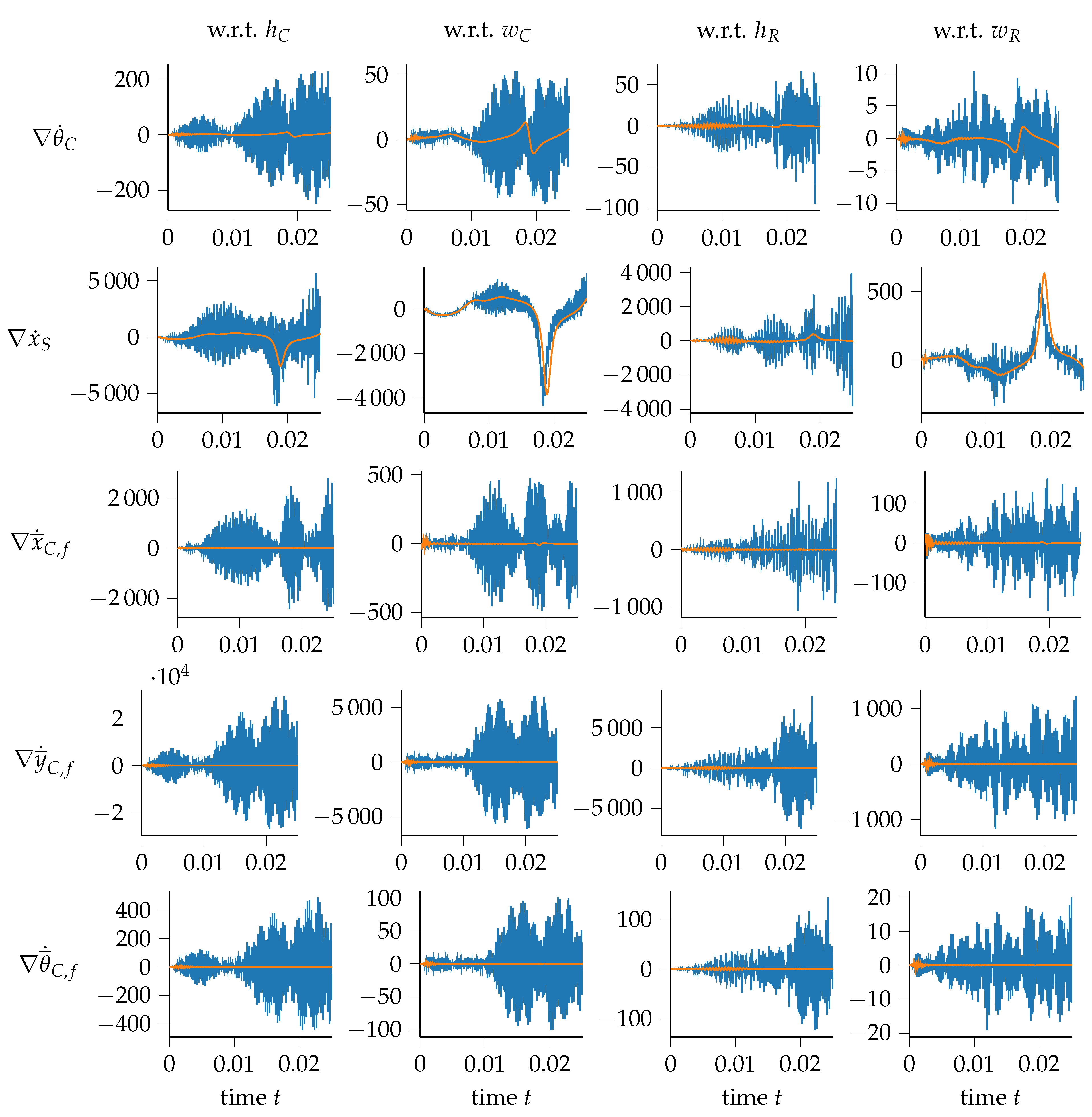
The results of the sensitivity analysis of the coordinates that are highlighted in Figure 8 are shown in Figure 12, Figure 13 and Figure 14. The analyzed coordinates include the rotation of the floating frame of the crank , the translation in the x direction of the floating frame of the slider and the three flexible coordinates of the node in A on the crank , and . The design variables used for the sensitivity analysis are the cross-sectional dimensions of the crank , and the rod , .
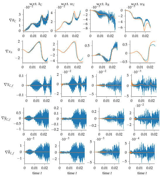
Figure 12.
Position sensitivities of the slider–crank mechanism with respect to , , and (values in MPa system of units, i.e., s, mm, , for translations and rad, , for rotations) calculated with —Newmark-β and —generalized-α compared with those numerically calculated via finite differencing with —Newmark-β and —generalized-α (undermost lines). Note: there is no visible difference between finite differencing and analytical sensitivities.
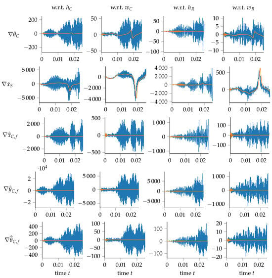
Figure 13.
Velocity sensitivities of the slider–crank mechanism with respect to , , and (values in MPa system of units, i.e., s, mm, , for translations and rad, , for rotations) calculated with —Newmark-β and —generalized-α compared with those calculated numerically via finite differencing with —Newmark-β and —generalized-α (undermost lines). Note: no visible difference between finite differencing and analytical sensitivities.
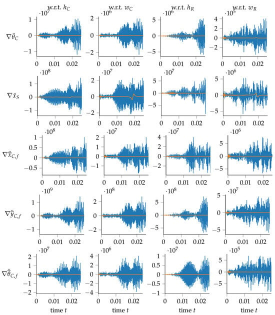
Figure 14.
Acceleration sensitivities of the slider–crank mechanism with respect to , , and (values in MPa system of units, i.e., s, mm, , for translations and rad, , for rotations) calculated with —Newmark-β and —generalized-α compared with those calculated numerically via finite differencing with —Newmark-β and —generalized-α (undermost lines). Note: there is no visible difference between finite differencing and analytical sensitivities.
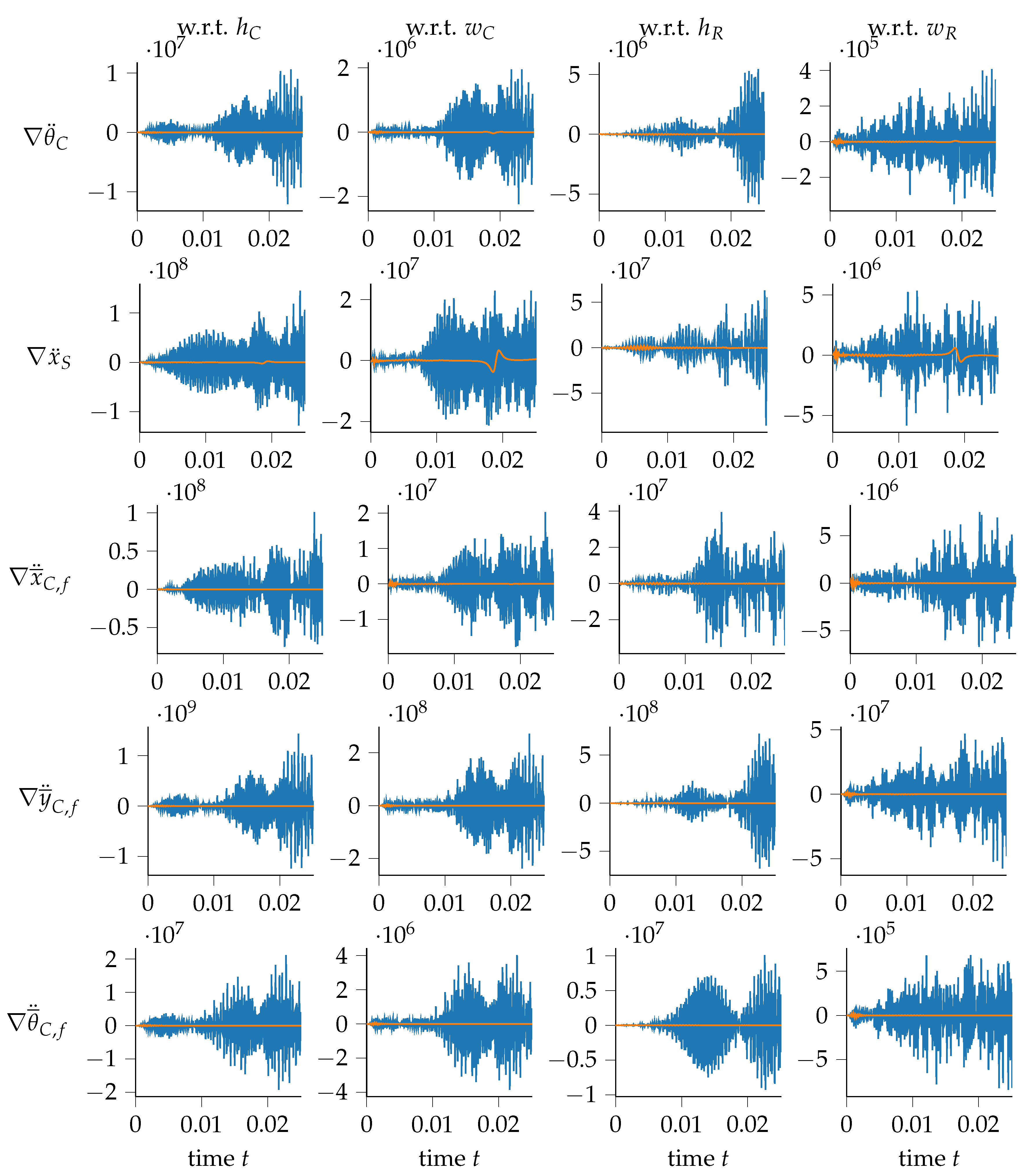
Similarly to the above, with Newmark-β, the results show a vibrating behavior that would lead to significant problems when using the sensitivities in gradient-based design optimization. With generalized-α, the numerical damping leads to usable sensitivity values after a few time steps. Figure 12 shows that the position sensitivities of the position and orientation coordinates of the floating frames are less noisy compared to the flexible coordinates.
Position sensitivities that suffer little from noise are limited to the position and orientation coordinates of the floating frames with respect to several design variables and include the following:
- sensitivities of with respect to and ;
- sensitivities of with respect to , , and .
Position sensitivities with significant noise include the position and orientation coordinates of the floating frames with respect to a few specific design variables as well as the flexible coordinates with respect to all design variables. The list of noisy responses of position sensitivities is given in the following:
- sensitivities of with respect to and ;
- sensitivities of with respect to ;
- sensitivities of with respect to , and ;
- sensitivities of with respect to ; , and ;
- sensitivities of with respect to , , and .
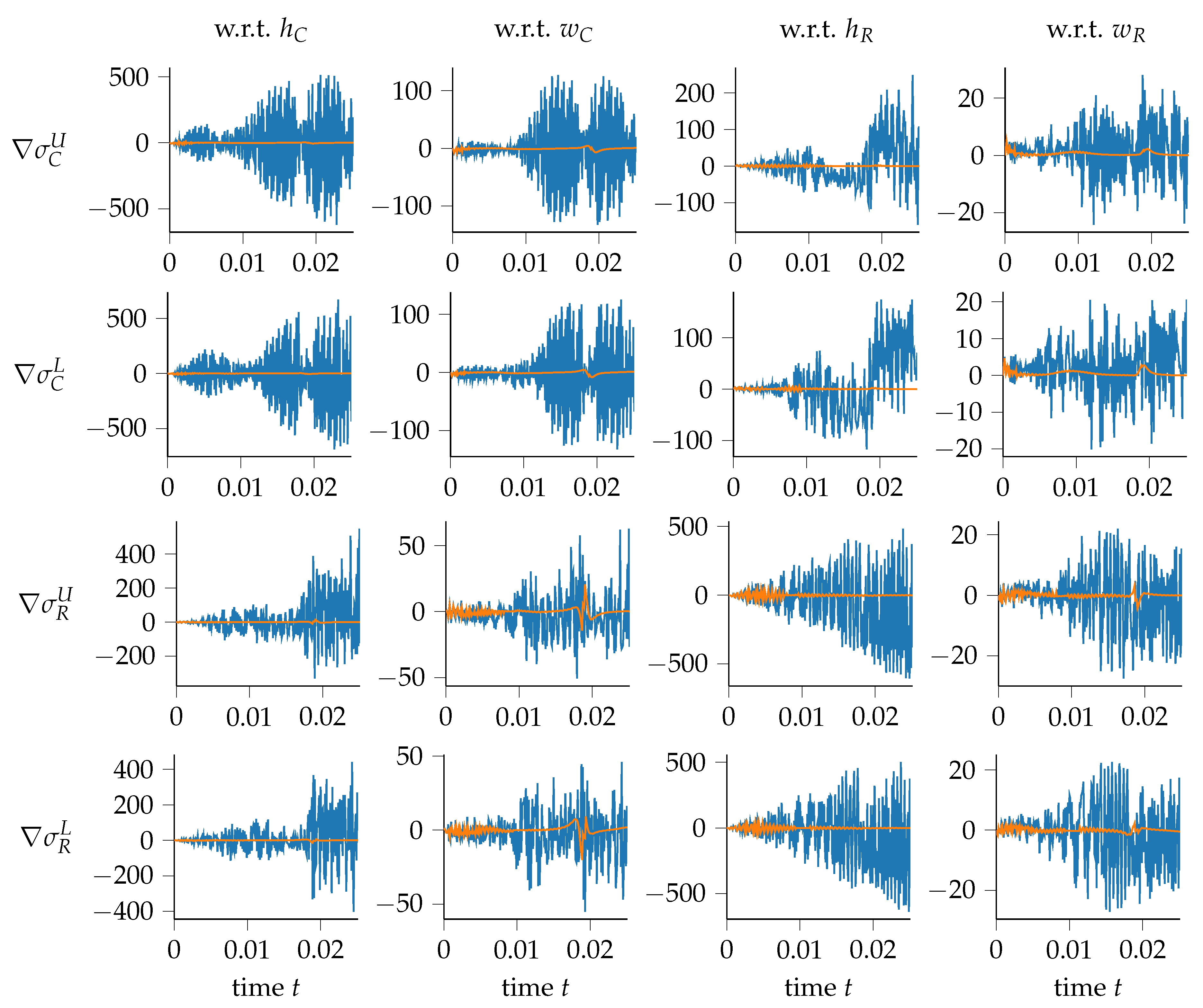
The sensitivities of the velocities as shown in Figure 13 and the sensitivities of the accelerations as shown in Figure 14 have noisy responses with Newmark that are damped with generalized-α for all investigated coordinates and all used design variables. The same behavior also continues with the sensitivity values for the maximum stresses in the crank and the rod shown in Figure 15.
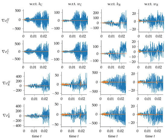
Figure 15.
Maximum stress sensitivities on the upper and lower fibers of the crank and the rod (values in MPa system of units, i.e., s, mm, , for translations and rad, , for rotations) calculated with —Newmark-β and —generalized-α compared with those calculated numerically via finite differencing with —Newmark-β and —generalized-α (undermost lines). Note: there is no visible difference between finite differencing and analytical sensitivities.
To check the correctness of the results, the sensitivity values with the introduced method are compared to numerical sensitivity analysis with forward differencing. The results are in good agreement, with only small numerical differences. In fact, there are no visible differences in Figure 12, Figure 13, Figure 14 and Figure 15 with the finite differencing values lying under the respective analytical values.
Table 4 shows a comparison of the computational effort with different methods. The computational effort with generalized-α is about lower compared to the computational effort with Newmark-β. The main reason for that is the continuing vibrating behavior with Newmark-β requires more iteration steps of the nonlinear solver. The comparison of the sensitivity methods with numerical finite differencing and analytical direct differentiation shows the high efficiency of the analytical method. With the four shown design variables, as shown in (63), an acceleration of about of the analytical method compared to the numerical method is obtained. The additional computational effort of analytical sensitivity analysis is just a fraction of the computational effort of the primal analysis. This is because of the simplification shown in (59), which also allows one to reuse the Jacobian matrix of the residual built in the primal analysis for the sensitivity analysis.

Table 4.
Computational effort for the slider–crank mechanism.
4. Conclusions
This work develops the analytical sensitivity analysis for the α-family of time integration, which has a single implementation for several common time integration schemes. This therefore has consequences for gradient-based optimization frameworks for dynamic systems. Analytical sensitivity analysis is crucial for efficient design optimization, parameter fitting and uncertainty analysis. In this work, the direct differentiation of the generalized-α time integration is derived and implemented for linear structural dynamics and flexible multibody dynamics, the latter of which requires a nonlinear solution routine. All equations needed for implementation are provided and extendable to further governing equations. The beneficial effects of the step-size-dependent numerical damping provided by the generalized-α method can clearly be seen in the comparison of the results with Newmark-β. The numerical noise of the responses and sensitivities can lead to convergence problems when using gradient-based optimization algorithms. This can be avoided when using the generalized-α time integration and its sensitivities as developed herein.
If the functions of interest are nonsmooth, discontinuous and bifurcated, non-gradient-based methods can be successfully used, e.g., design cases with crash analysis. Such cases can be solved with gradient-free optimization algorithms (e.g., [75,76,77]) and approximation methods (e.g., [78,79,80]).
The system responses with respect to the design variables are indeed often smooth, continuous and unbifurcated and thus enabling gradient-based methods where efficient and accurate sensitivity analysis is critical for both effectiveness and efficiency. This is shown above with linear structural dynamics and flexible multibody dynamics. The method and equations developed herein are of general nature and are extendable to further formulations and applicable to larger problems, both of larger number of degrees of freedom and number of design variables. Future investigations are needed on these large-scale problems to assess the acceleration and include a comparison with the adjoint variable method.
With the above study and introduction of the direct differentiation of the α-family of time integrators, the authors hope to provide the readers as design engineers a tool in the pursuit of optimal structures and mechanisms under dynamic loading.
Author Contributions
Conceptualization, E.W. and V.G.; methodology, E.W. and V.G.; software, E.W. and V.G.; validation, E.W. and V.G.; formal analysis, E.W. and V.G.; investigation, E.W. and V.G.; resources, E.W. and V.G.; data curation, E.W. and V.G.; writing—original draft preparation, E.W. and V.G.; writing—review and editing, E.W. and V.G.; visualization, E.W. and V.G.; supervision, E.W.; project administration, E.W.; funding acquisition, E.W. All authors have read and agreed to the published version of the manuscript.
Funding
This work is supported by the project CRC 2017 TN2091 doloMULTI Design of Lightweight Optimized structures and systems under MULTIdisciplinary considerations through integration of MULTIbody dynamics in a MULTIphysics framework, funded by the Free University of Bozen-Bolzano.
Data Availability Statement
Data available upon request.
Conflicts of Interest
The authors declare no conflicts of interest. The numerical studies by the first author were carried out during his previous position at the Free University of Bozen-Bolzano.
Appendix A. Derivation of Effective Equations of Motion for Structural Dynamics
Appendix A.1. Primal Analysis
The base for the α-family of integration methods is the equation of motion which for linear structural dynamics which is given by
and the intermediate values shown in Equations (3)–(5). Inserting the intermediate values into the equation of motion leads to
With Newmark’s equation, (1) and (2), this becomes
This can be rearranged in the following form
Therefore, the effective equation of motion is defined by
where
Appendix A.2. Sensitivity Analysis
The governing equation for sensitivities is the first derivative of the equation of motion,
where we introduce the intermediate sensitivity values (10)–(12),
and which we update with Newmark’s sensitivity Equations (16) and (17)
This equation can be rearranged to the following form,
Therefore, the effective equation of motion for sensitivities is defined by
where is given by Equation (A6) and the pseudo load is defined by
Appendix B. Derivation of Effective Equations of Motion for Flexible Multibody Dynamics
Appendix B.1. Primal Analysis
The base of the generalized-α method for index-1 differential algebraic equations of a flexible multibody system is given by
The intermediate point approximations of the force terms acting on the flexible multibody system are given by
Applying these linear approximations of the generalized-α method to the equations of motion leads to
Inserting Newmark’s Equations (1) and (2) gives
which can be rewritten to
The equations of motion of the effective system are given by
where
Appendix B.2. Nonlinear Solver
The base for the nonlinear solver are the residual equations of the flexible multibody system, given by
The Newton–Raphson method is used here
where the terms of the Jacobian matrix are given by
The derivatives of the system parameters of the previous time step with respect to the state variables of the next time step disappear,
The dependencies of the system parameters are shown in (33) and (34), and applying the chain rule of differentiation leads to
The derivatives of the state variables with respect to and are given by
Applying Equation (A42), Equations (A43)–(A51) lead to the terms of the Jacobian matrix given by
Appendix B.3. Sensitivity Analysis
The derivative of the equations of motion leads to the governing equation of the sensitivities given by
and
Including Newmark’s sensitivity, Equations (16) and (17) lead to
and
which can be rewritten to
and
The governing equation of the sensitivity analysis of the effective system is given by
where
References
- Hien, T.D.; Kleiber, M. Stochastic design sensitivity in structural dynamics. Int. J. Numer. Methods Eng. 1991, 32, 1247–1265. [Google Scholar] [CrossRef]
- Cho, S.; Choi, K.K. Design sensitivity analysis and optimization of non-linear transient dynamics. Part I–sizing design. Int. J. Numer. Methods Eng. 2000, 48, 351–373. [Google Scholar] [CrossRef]
- Cho, S.; Choi, K.K. Design sensitivity analysis and optimization of non-linear transient dynamics. Part II–configuration design. Int. J. Numer. Methods Eng. 2000, 48, 375–399. [Google Scholar] [CrossRef]
- van Keulen, F.; Haftka, R.; Kim, N. Review of options for structural design sensitivity analysis—Part 1: Linear systems. Comput. Methods Appl. Mech. Eng. 2005, 194, 3213–3243. [Google Scholar] [CrossRef]
- Martins, J.R.R.A.; Hwang, J.T. Review and unification of methods for computing derivatives of multidisciplinary computational models. AIAA J. 2013, 51, 2582–2599. [Google Scholar] [CrossRef]
- Tortorelli, D.A.; Michaleris, P. Design sensitivity analysis: Overview and review. Inverse Probl. Eng. 1994, 1, 71–105. [Google Scholar] [CrossRef]
- Wehrle, E.; Gufler, V. Lightweight engineering design of nonlinear dynamic systems with gradient-based structural design optimization. In Proceedings of the Munich Symposium on Lightweight Design 2020; Springer: Berlin/Heidelberg, Germany, 2021; pp. 44–57. [Google Scholar] [CrossRef]
- Wehrle, E. Optimal lightweight engineering via a three-block solver scheme for mechanical analysis. In Optimal Design and Control of Multibody Systems; Nachbagauer, K., Held, A., Eds.; Springer: Berlin/Heidelberg, Germany, 2024; Volume 42, pp. 16–29. [Google Scholar] [CrossRef]
- Courant, R.; Friedrichs, K.; Lewy, H. Über die partiellen Differenzengleichungen der mathematischen Physik. Math. Ann. 1928, 100, 32–74. [Google Scholar] [CrossRef]
- Newmark, N.M. A method of computation for structural dynamics. J. Eng. Mech. 1959, 85, 67–94. [Google Scholar] [CrossRef]
- Hilber, H.M.; Hughes, T.J.R.; Taylor, R.L. Improved numerical dissipation for time integration algorithms in structural dynamics. Earthq. Eng. Struct. Dyn. 1977, 5, 283–292. [Google Scholar] [CrossRef]
- Wood, W.L.; Bossak, M.; Zienkiewicz, O.C. An alpha modification of Newmark’s method. Int. J. Numer. Methods Eng. 1980, 15, 1562–1566. [Google Scholar] [CrossRef]
- Chung, J.; Hulbert, G.M. A time integration algorithm for structural dynamics with improved numerical dissipation: The generalized-α method. J. Appl. Mech. 1993, 60, 371–375. [Google Scholar] [CrossRef]
- Gufler, V.; Wehrle, E.; Vidoni, R. Sensitivity analysis of flexible multibody dynamics with generalized-α time integration and Baumgarte stabilization: A study on numerical stability. In Mechanisms and Machine Science; Springer International Publishing: Berlin/Heidelberg, Germany, 2022; pp. 147–155. [Google Scholar] [CrossRef]
- Griewank, A.; Walther, A. Evaluating Derivatives: Principles and Techniques of Algorithmic Differentiation, 2nd ed.; SIAM: Philadelphia, PA, USA, 2008. [Google Scholar]
- Naumann, U. The Art of Differentiating Computer Programs: An Introduction to Algorithmic Differentiation; SIAM: Philadelphia, PA, USA, 2012. [Google Scholar]
- Callejo, A.; Dopico, D. Direct sensitivity analysis of multibody systems: A vehicle dynamics benchmark. J. Comput. Nonlinear Dyn. 2019, 14, 021004. [Google Scholar] [CrossRef]
- Margossian, C.C. A review of automatic differentiation and its efficient implementation. WIREs Data Min. Knowl. Discov. 2019, 9, e1305. [Google Scholar] [CrossRef]
- Pi, T.; Zhang, Y.; Chen, L. First order sensitivity analysis of flexible multibody systems using absolute nodal coordinate formulation. Multibody Syst. Dyn. 2012, 27, 153–171. [Google Scholar] [CrossRef]
- Held, A.; Knüfer, S.; Seifried, R. Structural sensitivity analysis of flexible multibody systems modeled with the floating frame of reference approach using the adjoint variable method. Multibody Syst. Dyn. 2016, 40, 287–302. [Google Scholar] [CrossRef]
- Boopathy, K.; Kennedy, G. Adjoint-based derivative evaluation methods for flexible multibody systems with rotorcraft applications. In Proceedings of the 55th AIAA Aerospace Sciences Meeting, Grapevine, TX, USA, 9–13 January 2017; American Institute of Aeronautics and Astronautics: Reston, VA, USA, 2017. [Google Scholar] [CrossRef]
- Martins, J.R.R.A.; Kennedy, G.J. Enabling large-scale multidisciplinary design optimization through adjoint sensitivity analysis. Struct. Multidiscip. Optim. 2021, 64, 2959–2974. [Google Scholar] [CrossRef]
- Nachbagauer, K.; Oberpeilsteiner, S.; Sherif, K.; Steiner, W. The use of the adjoint method for solving typical optimization problems in multibody dynamics. J. Comput. Nonlinear Dyn. 2015, 10, 061011. [Google Scholar] [CrossRef]
- Lauß, T.; Oberpeilsteiner, S.; Steiner, W.; Nachbagauer, K. The discrete adjoint method for parameter identification in multibody system dynamics. Multibody Syst. Dyn. 2017, 42, 397–410. [Google Scholar] [CrossRef]
- Boopathy, K.; Kennedy, G.J. Parallel finite element framework for rotorcraft multibody dynamics and discrete adjoint sensitivities. Aiaa J. 2019, 57, 3159–3172. [Google Scholar] [CrossRef]
- Boopathy, K. Adjoint Based Design Optimization of Systems with Time Dependent Physics and Probabilistically Modeled Uncertainties. Ph.D. Thesis, Georgia Institute of Technology, Atlanta, GA, USA, 2020. [Google Scholar]
- Ebrahimi, M.; Butscher, A.; Cheong, H.; Iorio, F. Design optimization of dynamic flexible multibody systems using the discrete adjoint variable method. Comput. Struct. 2019, 213, 82–99. [Google Scholar] [CrossRef]
- Nejat, A.A.; Moghadasi, A.; Held, A. Adjoint sensitivity analysis of flexible multibody systems in differential-algebraic form. Comput. Struct. 2020, 228, 106–148. [Google Scholar] [CrossRef]
- Held, A. On design sensitivities in the structural analysis and optimization of flexible multibody systems. Multibody Syst. Dyn. 2022, 54, 53–74. [Google Scholar] [CrossRef]
- Solano, D.; Sarojini, D.; Rajaram, D.; Mavris, D.N. Adjoint-based analysis and optimization of beam-like structures subjected to dynamic loads. Struct. Multidiscip. Optim. 2022, 65, 52. [Google Scholar] [CrossRef]
- Haug, E.J.; Arora, J.S. Design sensitivity analysis of elastic mechanical systems. Comput. Methods Appl. Mech. Eng. 1978, 15, 35–62. [Google Scholar] [CrossRef]
- Hsieh, C.C.; Arora, J.S. Structural design sensitivity analysis with general boundary conditions: Dynamic problem. Int. J. Numer. Methods Eng. 1985, 21, 267–283. [Google Scholar] [CrossRef]
- Baier, H.; Seeßelberg, C.; Specht, B. Optimierung in der Strukturmechanik; Vieweg: Braunschweig/Wiesbaden, Germany, 1994. [Google Scholar] [CrossRef]
- Trier, S.; Marthinsen, A.; Sivertsen, O. Design sensitivities by the adjoint variable method in nonlinear structural dynamics. In Proceedings of the SIMS Simulation Conference, Trondheim, Norway, 11–13 June 1996. [Google Scholar]
- Michaleris, P.; Tortorelli, D.A.; Vidal, C.A. Tangent operators and design sensitivity formulations for transient non-linear coupled problems with applications to elastoplasticity. Int. J. Numer. Methods Eng. 1994, 37, 2471–2499. [Google Scholar] [CrossRef]
- Bhalerao, K.D.; Poursina, M.; Anderson, K.S. An efficient direct differentiation approach for sensitivity analysis of flexible multibody systems. Multibody Syst. Dyn. 2010, 23, 121–140. [Google Scholar] [CrossRef]
- Zhu, Y. Sensitivity Analysis and Optimization of Multibody Systems. Ph.D. Thesis, Virginia Polytechnic Institute and State University, Blacksburg, VA, USA, 2014. [Google Scholar]
- Dopico, D.; Zhu, Y.; Sandu, A.; Sandu, C. Direct and adjoint sensitivity analysis of ordinary differential equation multibody formulations. J. Comput. Nonlinear Dyn. 2014, 10, 011012. [Google Scholar] [CrossRef]
- Callejo, A.; Sonneville, V.; Bauchau, O. Discrete adjoint method for the sensitivity analysis of flexible multibody systems. J. Comput. Nonlinear Dyn. 2018, 14, 021001. [Google Scholar] [CrossRef]
- Cao, Z.; Yao, J.; Jia, Z.; Liang, D. Transient response sensitivity analysis of localized nonlinear structure using direct differentiation method. Machines 2022, 10, 1039. [Google Scholar] [CrossRef]
- Haug, E.J.; Ehle, P.E. Second-order design sensitivity analysis of mechanical system dynamics. Int. J. Numer. Methods Eng. 1982, 18, 1699–1717. [Google Scholar] [CrossRef]
- Ding, J.Y.; Pan, Z.K.; Chen, L.Q. Second order adjoint sensitivity analysis of multibody systems described by differential-algebraic equations. Multibody Syst. Dyn. 2007, 18, 599–617. [Google Scholar] [CrossRef]
- Belotti, R.; Palomba, I.; Wehrle, E.; Vidoni, R. An approximation-based design optimization approach to eigenfrequency assignment for flexible multibody systems. Appl. Sci. 2021, 11, 11558. [Google Scholar] [CrossRef]
- Palomba, I.; Vidoni, R. Flexible-link multibody system eigenvalue analysis parameterized with respect to rigid-body motion. Appl. Sci. 2019, 9, 5156. [Google Scholar] [CrossRef]
- Brüls, O.; Lemaire, E.; Duysinx, P.; Eberhard, P. Multibody dynamics. In Multibody Dynamics: Computational Methods and Applications; Arczewski, K., Blajer, W., Fraczek, J., Wojtyra, M., Eds.; Springer: Berlin/Heidelberg, Germany, 2011; Chapter Optimization of Multibody Systems and Their Structural Components; pp. 49–68. [Google Scholar] [CrossRef]
- Gufler, V.; Wehrle, E.; Vidoni, R. Multiphysical design optimization of multibody systems: Application to a Tyrolean weir cleaning mechanism. In Proceedings of the 3rd International Conference of IFToMM Italy, Naples, Italy, 9–11 September 2020. [Google Scholar] [CrossRef]
- Gufler, V.; Wehrle, E.; Achleitner, J.; Vidoni, R. A semi-analytical approach to sensitivity analysis with flexible multibody dynamics of a morphing forward wing section. Multibody Syst. Dyn. 2023, 58, 1–20. [Google Scholar] [CrossRef]
- Gufler, V.; Zwölfer, A.; Wehrle, E. Analytical derivatives of flexible multibody dynamics with the floating frame of reference formulation. Multibody Syst. Dyn. 2022, 60, 257–288. [Google Scholar] [CrossRef]
- Brüls, O.; Golinval, J. The generalized-α method in mechatronic applications. ZAMM 2006, 86, 748–758. [Google Scholar] [CrossRef]
- Jansen, K.E.; Whiting, C.H.; Hulbert, G.M. A generalized-α method for integrating the filtered Navier–Stokes equations with a stabilized finite element method. Comput. Methods Appl. Mech. Eng. 2000, 190, 305–319. [Google Scholar] [CrossRef]
- Köbis, M.A.; Arnold, M. Convergence of generalized-α time integration for nonlinear systems with stiff potential forces. Multibody Syst. Dyn. 2015, 37, 107–125. [Google Scholar] [CrossRef]
- Bestle, D. Analyse und Optimierung von Mehrkörpersystemen; Springer: Berlin/Heidelberg, Germany, 1994. [Google Scholar] [CrossRef]
- Haug, E.J.; Arora, J.S. Applied Optimal Design: Mechanical and Structural Systems; John Wiley & Sons: Hoboken, NJ, USA, 1979. [Google Scholar]
- Gufler, V.; Wehrle, E.; Zwölfer, A. A review of flexible multibody dynamics for gradient-based design optimization. Multibody Syst. Dyn. 2021, 53, 379–409. [Google Scholar] [CrossRef]
- Shabana, A.A. Flexible multibody dynamics: Review of past and recent developments. Multibody Syst. Dyn. 1997, 1, 189–222. [Google Scholar] [CrossRef]
- Shabana, A.A. Dynamics of Multibody Systems, 3rd ed.; Cambridge University Press: Cambridge, UK, 2013. [Google Scholar] [CrossRef]
- Petzold, L.; Lötstedt, P. Numerical solution of nonlinear differential equations with algebraic constraints II: Practical implications. SIAM J. Sci. Stat. Comput. 1986, 7, 720–733. [Google Scholar] [CrossRef]
- Bottasso, C.L.; Bauchau, O.A.; Cardona, A. Time-step-size-independent conditioning and sensitivity to perturbations in the numerical solution of index three differential algebraic equations. SIAM J. Sci. Comput. 2007, 29, 397–414. [Google Scholar] [CrossRef][Green Version]
- Bauchau, O.A. Flexible Multibody Dynamics; Springer: Berlin/Heidelberg, Germany, 2011. [Google Scholar] [CrossRef]
- Dopico, D.; González, F.; Luaces, A.; Saura, M.; García-Vallejo, D. Direct sensitivity analysis of multibody systems with holonomic and nonholonomic constraints via an index-3 augmented Lagrangian formulation with projections. Nonlinear Dyn. 2018, 93, 2039–2056. [Google Scholar] [CrossRef]
- Baumgarte, J. Stabilization of constraints and integrals of motion in dynamical systems. Comput. Methods Appl. Mech. Eng. 1972, 1, 1–16. [Google Scholar] [CrossRef]
- Gufler, V.; Wehrle, E.; Vidoni, R. Analytical sensitivity analysis of flexible multibody dynamics with index-1 differential-algebraic equations and Baumgarte stabilization. Int. J. Mech. Control 2023, 24, 3–14. [Google Scholar]
- Arnold, M.; Brüls, O. Convergence of the generalized-α scheme for constrained mechanical systems. Multibody Syst. Dyn. 2007, 18, 185–202. [Google Scholar] [CrossRef]
- Bathe, K.J.; Noh, G. Insight into an implicit time integration scheme for structural dynamics. Comput. Struct. 2012, 98–99, 1–6. [Google Scholar] [CrossRef]
- Huang, C.; Fu, M. A composite collocation method with low-period elongation for structural dynamics problems. Comput. Struct. 2018, 195, 74–84. [Google Scholar] [CrossRef]
- Kadapa, C.; Dettmer, W.; Perić, D. On the advantages of using the first-order generalised-alpha scheme for structural dynamic problems. Comput. Struct. 2017, 193, 226–238. [Google Scholar] [CrossRef]
- Malakiyeh, M.M.; Shojaee, S.; Javaran, S.H. Development of a direct time integration method based on Bezier curve and 5th-order Bernstein basis function. Comput. Struct. 2018, 194, 15–31. [Google Scholar] [CrossRef]
- Namadchi, A.H.; Jandaghi, E.; Alamatian, J. A new model-dependent time integration scheme with effective numerical damping for dynamic analysis. Eng. Comput. 2020, 37, 2543–2558. [Google Scholar] [CrossRef]
- Noh, G.; Bathe, K.J. The Bathe time integration method with controllable spectral radius: The ρ∞-Bathe method. Comput. Struct. 2019, 212, 299–310. [Google Scholar] [CrossRef]
- Shojaee, S.; Rostami, S.; Abbasi, A. An unconditionally stable implicit time integration algorithm: Modified quartic B-spline method. Comput. Struct. 2015, 153, 98–111. [Google Scholar] [CrossRef]
- Wen, W.; Wei, K.; Lei, H.; Duan, S.; Fang, D. A novel sub-step composite implicit time integration scheme for structural dynamics. Comput. Struct. 2017, 182, 176–186. [Google Scholar] [CrossRef]
- Bathe, K.J. Finite Element Procedures; Prentice Hall: Englewood Cliffs, NJ, USA, 1996; p. 1037. [Google Scholar]
- Kreisselmeier, G.; Steinhauser, R. Systematic control design by optimizing a vector performance index. In Proceedings of the International Federation of Active Controls Symposium on Computer-Aided Design of Control Systems, Zürich, Switzerland, 29–31 August 1979. [Google Scholar] [CrossRef]
- Martins, J.R.R.A.; Poon, N.M.K. On structural optimization using constraint aggregation. In Proceedings of the 6th World Congress on Structural and Multidisciplinary Optimization, Rio de Janeiro, Brazi, 30 May–3 June 2005. [Google Scholar]
- Duddeck, F. Multidisciplinary optimization of car bodies. Struct. Multidiscip. Optim. 2008, 35, 375–389. [Google Scholar] [CrossRef]
- Kurtaran, H.; Eskandarian, A.; Marzougui, D.; Bedewi, N.E. Crashworthiness design optimization using successive response surface approximations. Comput. Mech. 2002, 29, 409–421. [Google Scholar] [CrossRef]
- Langer, H. Extended Evolutionary Algorithms for Multiobjective and Discrete Design Optimization of Structure. Ph.D. Dissertation, Lehrstuhl für Leichtbau, Technische Universität München, Munich, Germany, 2005. [Google Scholar]
- Boursier Niutta, C.; Wehrle, E.J.; Duddeck, F.; Belingardi, G. Surrogate modeling in design optimization of structures with discontinuous responses: A new approach for ill-posed problems in crashworthiness design. Struct. Multidiscip. Optim. 2018, 57, 1857–1869. [Google Scholar] [CrossRef]
- Forrester, A.I.J.; Sábester, A.; Keane, A.J. Engineering Design via Surrogate Modelling: A Practical Guide; Wiley: Hoboken, NJ, USA, 2008; p. 227. [Google Scholar]
- Xu, Q.; Wehrle, E.; Baier, H. Knowledge-based surrogate modeling in engineering design optimization. In Surrogate-Based Modeling and Optimization; Koziel, S., Leifsson, L., Eds.; Springer: Berlin/Heidelberg, Germany, 2013; pp. 313–336. [Google Scholar] [CrossRef]
Disclaimer/Publisher’s Note: The statements, opinions and data contained in all publications are solely those of the individual author(s) and contributor(s) and not of MDPI and/or the editor(s). MDPI and/or the editor(s) disclaim responsibility for any injury to people or property resulting from any ideas, methods, instructions or products referred to in the content. |
© 2024 by the authors. Licensee MDPI, Basel, Switzerland. This article is an open access article distributed under the terms and conditions of the Creative Commons Attribution (CC BY) license (https://creativecommons.org/licenses/by/4.0/).


