Abstract
Data-based equipment fault detection and diagnosis is an important research area in the smart factory era, which began with the Fourth Industrial Revolution. Steel manufacturing is a typical processing industry, and efficient equipment operation can improve product quality and cost. Steel production systems require precise control of the equipment, which is a complex process. A gearbox transmits power between shafts and is an essential piece of mechanical equipment. A gearbox malfunction can cause serious problems not only in production, quality, and delivery but in safety. Many researchers are developing methods for monitoring gearbox condition and for diagnosing failures in order to resolve problems. In most data-driven methods, the analysis data set is derived from a distribution of identical data with failure mode labels. Industrial sites, however, often collect data without information on the failure type or failure status due to varying operating conditions and periodic repair. Therefore, the data sets not only include frequent false alarms, but they cannot explain the causes of the alarms. In this paper, a framework called the Reduced Lagrange Method (R-LM) periodically assigns pseudolabels to vibration signals collected without labels and creates an input data set. In order to monitor the status of equipment and to diagnose failures, the input data set is fed into a supervised learning classifier. To verify the proposed method, we build a test rig using motors and gearboxes that are used on production sites in order to artificially simulate defects in the gears and to operate them to collect vibration data. Data features are extracted from the frequency domain and time domain, and pseudolabeling is applied. There were fewer false alarms when applying R-LM, and it was possible to explain which features were responsible for equipment status changes, which improved field applicability. It was possible to detect changes in equipment conditions before a catastrophic failure, thus providing meaningful alarm and warning information, as well as further promising research topics.
1. Introduction
To produce steel products, the steel industry requires a complex production system with multiple types of equipment and precise control. Integrated steelworks, in particular, operate in harsh environments with high temperatures and pressure, as well as a lot of dust and moisture. There are significant economic losses if an unplanned shutdown happens in steel production equipment, thereby adversely affecting product quality, delivery, and safety. Therefore, it is crucial to detect equipment anomalies early and handle them proactively before catastrophic failures. The steel industry spends 10% to 20% of its production costs on equipment maintenance, so minimizing unplanned breakdowns is essential [1,2].
There was USD 4.9 trillion worth of physical assets in the US steel industry. Average maintenance spending was between 5% and 8% of total costs, with the best performers spending less than 2% to 3%. The steel industry wastes more than USD 180 billion in excess maintenance spending annually. According to the Federal Energy Management Program, predictive maintenance can save 8% to 12% more than is saved with preventive maintenance (PM). Furthermore, predictive maintenance has been shown to recover 10% of investment costs, thus reducing maintenance costs by 25%, reducing unplanned shutdowns by 70%, reducing downtime by 45%, and improving productivity by 25% [3].
A gearbox is a fundamental component of rotating machinery that transmits power between the shafts used in steel mills, power turbines, automobiles, and airplanes. As a result, fault detection and diagnosis (FDD) for gearboxes is essential to prevent mechanical malfunctions that could damage the systems. Among single-equipment failures, gearbox-related failures were found to be the highest in one steel company at 38%. As the types of steel produced become more diverse, machines operate at higher loads than they were designed for. A sudden failure of a gearbox can cause quality defects, expensive repairs, and even accidents. The health of a gearbox can be confirmed by measuring the vibrations, acoustics, heat, and iron content in lubricants. Among these, vibration signals are the most widely used because they contain a lot of information from inside the mechanical equipment. In order to monitor gearbox conditions and detect defects early, various technologies such as artificial intelligence and signal processing are being researched [4,5,6,7,8,9,10,11,12,13].
It is crucial to maintain desirable performance in industrial processes where a variety of faults can occur. For most industries, FDD is an important control method because better processing performance is expected from improving the FDD capability. There are two main functions [14]:
- Monitoring the behavior of a process (variables);
- Identifying faults, their characteristics, and their root causes.
As early as the 1970s, equipment condition monitoring and diagnosis attracted interest and research, but the original data did not allow for effective equipment maintenance policy decision making. In the 1980s, breakdown maintenance (BM) dominated, and PM followed in the 1990s. Since 2000, condition-based maintenance (CBM) and prognostics and health management have become mainstream. In recent years, smart technologies such as the IoT, machine learning (ML), and artificial intelligence (AI) have made it possible to collect and store large amounts of data at very low costs, and computing power has skyrocketed with parallel processing in GPUs. The equipment maintenance environment is undergoing a major transformation due to improvements. According to the German National Academy of Science and Engineering, the Fourth Industrial Revolution (Industry 4.0) will increase industrial productivity by 30%. It is essential to establish an economical equipment maintenance policy in light of this paradigm shift in manufacturing [15,16,17]. In particular, steel manufacturing equipment must be reliable and must have a long lifespan to reduce economic losses due to unplanned breakdowns. With the help of the IoT, big data, and AI, it is possible to monitor and predict the status of equipment. In accordance with changes in the industrial environment, methods in and perspectives on equipment maintenance strategy have changed and are more important today than ever. On real industrial sites, most companies perform BM and PM, not proactive and predictive maintenance. According to survey results, predictive maintenance is only carried out for certain core equipment, and companies want to invest time and resources in it, but the majority of resources are used for preventive and breakdown maintenance instead [18].
The steel manufacturing industry generates and stores large amounts of data on their equipment for efficient maintenance, but it is difficult to use these data to maintain equipment. The reasons are as follows.
- Steel-making plants continually switch between a load state (where they exert force for processing) and an idle state where they do not. Without a distinction between equipment operating conditions, it is difficult to detect changes in equipment status from the collected data. This difficulty can be overcome by eliminating noise in the data, recording the exact time of an occurrence (time stamping), and compiling event data.
- The data collected in the field on vibrations, temperatures, electric current, and debris inside the oil are often collected separately from the meta data (event data) that indicate the equipment’s operating condition. The equipment data collected cannot be labeled as failure or normal states, thus making it difficult to apply a supervised learning algorithm.
- When parts of the equipment are replaced, overhauled, or repaired, the characteristics of that equipment are altered. Because of this, the data on equipment status are not accurate, so they must be collected again to reflect the current normal status.
In a steel production site, it is unlikely that the same failure mode will occur multiple times in a short period of time. Additionally, failure diagnosis research can be carried out on a small laboratory-scale test rig, but there is a problem in that monitoring and diagnosing the condition of equipment actually operating in the field is difficult. We propose a pseudolabel method for monitoring and diagnosing equipment status changes using the powerful classification performance of supervised learning. We then show that equipment abnormalities can be diagnosed and monitored through the classification of data collected from actual field equipment.
In summary, this study has the following contributions:
- Unlabeled vibration data can be pseudolabeled and used to monitor changes in equipment conditions using a supervised learning classifier.
- It is possible to reduce false alarms due to periodic changes in equipment operating under normal conditions.
- We confirm the timing of equipment condition changes.
- A quantitative analysis was performed, and relationships between independent and dependent variables are explained to determine which features affect equipment abnormalities.
This paper is organized as follows. Section 2 presents related work. In Section 3, we explain the equipment condition monitoring procedure and present the algorithm for it. The theoretical background for the method in this paper is introduced in Section 4. The experimental setting and results are reported in Section 5. Finally, Section 6 presents a discussion and our conclusion.
2. Related Work
One steel manufacturing company investigated more than 1000 equipment failures over two years in order to analyze equipment diagnosis. They found that 22% of the inspections were inadequate, 21% required detailed equipment diagnosis (e.g., for gear wear due to equipment fatigue), 17% were regular inspections for damage to gearboxes and bearings, and 17% of the failures were due to an insufficient number of inspections. Insufficient replacements accounted for 5% of failures, while failures that could not be predicted, such as internal leaks in hydraulic cylinders, the deterioration of semiconductor materials, and natural disasters, accounted for 35%. Through equipment inspections and monitoring, 65% of all failures could be prevented, and equipment status information could be comprehensively analyzed through equipment condition monitoring and diagnosis to determine the optimal maintenance time before an equipment failure occurs. An economic equipment maintenance strategy can be developed to prevent unplanned equipment breakdowns.
Kumar [4] analyzed comprehensive CBM. They classified methods into those for vibration, noise, debris from wear, and temperature, and they emphasized the importance of vibration analysis by introducing various features in the time domain and frequency domain, along with their physical interpretations. According to existing research, supervised learning techniques are used 88% of the time when analyzing equipment failure data, and unsupervised learning techniques are used 12% of the time [15]. Under supervised learning, fault identification studies are conducted based on labels indicating whether or not faults exist in the data. The purpose of unsupervised learning is to detect anomalies. A regression model was constructed to analyze abnormal conditions on ships and changes detected with unlabeled data through statistical methods, such as regression analysis, time series analysis, and probabilistic models.
Tran and Yang [14] pointed out the limitations of existing approaches in failing to consider a comprehensive system. Several industrial applications were evaluated by using two case studies to propose intelligent CBM for rotating machinery. There are a number of studies based on classification using support vector machines (SVMs) to monitor, diagnose, and predict abnormalities in equipment. Various patterns can be found with an SVM, and the extracted patterns can be classified into fault types based on their features. Using SVM approaches for monitoring machine status and diagnosing faults, Widodo and Yang [19] discussed future developments in SVMs, which are more expertise- or problem-oriented. Banerjee and Das [20] discussed a fault diagnosis problem for dynamic motor conditions. They developed an approach for classifying fault signals by combining information extracted with an SVM and short-term Fourier transform (STFT) based on data obtained from multiple sensors. Park et al. [21] proposed a new approach to fault detection and extraction based on a cubic spline regression method, which was used to find step changing points, and SVM algorithms were used to build a classifier. In particular, they considered coefficient parameters multiplied by each cubic spline regression of the process features, which were then used as input for the development of the classifier. Wang et al. [22] proposed a method for diagnosing ball bearing abnormalities using a SVM and Mahalanobis distance. Shin et al. [23] proposed anomaly detection in a high dimension using a support vector machine to find the hyperplane of the maximum margin in high-dimensional space.
There are numerous steps involved in developing a machine learning model and implementing it in actual operations. It requires experts from diverse fields to define the problem, collect data, preprocess the data, develop the model, evaluate it, and apply it to the service. In auto-ML, inefficient tasks are automated as much as possible so that productivity and efficiency are increased as often as possible. In particular, research has been conducted for a long time on technologies that can effectively develop high-quality models by minimizing model developer intervention in the processes from data preprocessing to algorithm selection and tuning [24,25,26]. With the development of auto-ML, defining the problem well and collecting the right data that accurately reflect reality are becoming more important than deciding which classifier to select.
Deep learning has rapidly replaced existing machine learning algorithms, such as SVMs and decision trees (DTs), as deep learning research began to produce results. Deep learning has spread rapidly because of its high performance and the ease in solving problems by automating feature engineering (the most important machine learning step). Machine learning requires the creation of good features from the data, whereas deep learning examines all the features concurrently. The use of the features of deep learning is being researched for monitoring and diagnosing equipment problems. Even though deep learning produces excellent results, we do not know how they are achieved. In order to overcome these limitations, explainable AI has been researched. In spite of excellent results, a learning model can only be made more usable if its interpretation can be improved. As a result, traditional methods that are easy to interpret must still be useful. Hong et al. [27] and Lu [28] proposed a new data fusion method based on physics-constrained dictionary learning to improve the efficiency of data collection and the accuracy of fault diagnosis. Miao et al. [29] proposed a sparse representation block that extracts the impulse component of the vibration signal and converts the time domain signal to the sparse domain through sparse mapping of the convolution graph.
Seo and Yun studied hot strip rolling mill equipment status and diagnosis [30,31]. The study reported in [30] used partitioning around medoids, a type of K-medoids clustering, for monitoring equipment status. Based on silhouette width, they quantified clustering performance and monitored the point when a new cluster captured abnormal equipment behavior. Seo and Yun also used an autoencoder (AE) to learn data assumed to be normal [32]. A method of monitoring equipment status was used to detect changes in AE model reconstruction errors after a data set of interest was inserted into the model. Due to the lack of labels in the data collected from the production site, an unsupervised learning method was chosen. To overcome these problems, Seo et al. [33] proposed a pseudolabeling method named the Lagrange Method for equipment monitoring. A labeled data set is used to diagnose equipment problems, which are then entered into a classifier, and the classification accuracy is monitored. The proposed method has a tendency, however, to generate alarms in sections considered normal and judging as abnormal some conditions that change periodically in accordance with equipment operations. Their proposed method also has a disadvantage in that it responds to accumulated changes in equipment condition. This means the possibility of false alarms is high, and it can be difficult to know about such changes in real time. Furthermore, there was no explanation for what variables were influential in cases where classification accuracy was high, which made it difficult to interpret the results intuitively. An improved pseudolabeling method is proposed in this paper that reduces false alarms and accurately captures changes in equipment status over time. It addresses the following issues:
- When an artificial failure is created, labeled, and then analyzed, it is unlikely to produce the same results in the field.
- When a methodology cannot be applied directly at the production site because only vibration signals are collected without normal presence-and-absence labels.
- When fault alarms are inevitable if the equipment characteristics include repeated accelerations, decelerations, and stopping while operating, and they are subject to temporary influences from the surrounding environment.
- When normal states of the equipment constantly change, whether because of regular repairs, overhauls, oil replenishment, or minor repairs.
The purpose of this paper is to demonstrate that pseudolabels can be applied to unlabeled time series data to create a classifier that monitors and diagnoses equipment abnormalities.
3. Equipment Condition Monitoring
3.1. The Proposed Reduced Lagrange Method
As shown in Figure 1a, the Lagrange Method (LM) can be expressed in a manner similar to a traditional recurrent neural network (RNN). The left side of the equal sign is the LM’s overall structure, which is illustrated by three blue arrows:
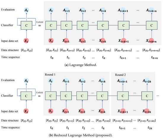
Figure 1.
The concepts of (a) the Lagrange Method and (b) the Reduced Lagrange Method.
- The first arrow indicates that the input data set is entered into the classifier (C). On the right side of Figure 1a, you can see the unfolded tasks for each time sequence. describes the structure of the input data set and refers to normal and abnormal data sets, respectively. Data set in the ith time sequence is labeled normal up front. Data set in the jth time sequence is labeled abnormal later. In the data structure, you can see that the first data sets are all the same, , which indicates that you have a data set that can be considered normal. The data sets prepared for each time sequence are considered abnormal and are used as input for the classifier.
- The second arrow indicates that the evaluation metric is created and stored in the classifier. A pseudolabeled data set is input, and the classifier stores the classification performance. represents the classification evaluation performance of the classifier at time sequence .
- The topmost arrows execute the classifier repeatedly. and denote the classifier and the nth time sequence, respectively.
Figure 1b illustrates the Reduced Lagrange Method (R-LM). Unlike the LM, data set , which is considered normal and pseudolabeled as normal, is used only k times as a normal data set. In the kth time sequence, the normal data set changes to and is maintained k times. Round 1 is denoted by , thereby maintaining a normal data set k times. For each time sequence, a predesigned data set is constructed and used as input for the classifier. Values for the classification performance metric (e.g., accuracy) generated by the classifier are saved and analyzed. The series of processes is repeated for each time sequence within a round. Each round has k repetitions, which must be determined by the user. A fixed data set that is pseudolabeled as normal is used k times within a round. In Round 1, the data structure of is a pseudonormal data set, which is used k times. This way, the fixed data set can be labeled as normal, and the next data set can be labeled as abnormal, thereby resulting in a data set that can be input into the classifier. No classifier will be able to differentiate between the two data sets if they are derived from the same homogeneous group. Data can be classified by using a classifier if equipment conditions change and the data in the data sets change. Classification accuracy will increase when equipment changes are large, so it can be used as a diagnostic tool to diagnose equipment problems. In order to determine k, the user must take into account the characteristics of the equipment and how quickly the alarm must sound. The LM does not set the k value, so it continues to use data from one point in the past as a normal label. There are limitations to this approach, because the range of normal states may shift periodically depending on operating conditions where field equipment repeats acceleration and deceleration. The normal data set from the equipment needs to reflect normal maintenance activities such as overhauls, minor repairs, and oil changes.
3.2. Procedure for Equipment Monitoring and Fault Detection
It is necessary to prepare an input data set in order to monitor the condition of the equipment. These are the data sets labeled normal (N) and abnormal (A) for input. The input data pair should be normalized so that the mean is 0 and the standard deviation is 1, and then the data set should be divided into training, validation, and testing data sets at a certain ratio. In order to calculate relative variable importance, use a random forest (RF) algorithm and sort in descending order. In order to train a classifier, the variables ranked in the top 10 are used. The evaluation metric should be calculated using testing data. For each time sequence, k classifier operations are performed, and the evaluation results are calculated. A normality test is performed on the data set that contains the evaluation results. A p value less than 0.05 suggests that the sample did not originate from a normal distribution, and, therefore, the equipment condition has changed. If the p value is greater than 0.05, we can say that it follows a normal distribution, meaning no characteristics have changed. If the average value of the accumulated evaluation result is greater than 0.7, an alert is generated; if it is greater than 0.8, an alarm is generated, and if it is greater than 0.9, a warning signal is generated. This content can be expressed with the Algorithm 1. Figure 2 shows the procedure for equipment monitoring and fault detection. First, after data acquisition, preprocessing is performed, and features are extracted. After performing pseudolabeling, the data set is divided into train, test, and validation data to learn a classification model and monitor equipment abnormalities by reviewing evaluation indicators.
| Algorithm 1 Procedure for equipment condition monitoring based on the R-LM |
| Input: |
| Input data set structure defined as . |
| where is a data set pseudolabeled normal in the ith time sequence. |
| is a data set pseudolabeled abnormal in the th time sequence. |
| For each iteration k: |
| is fixed during k iterations |
| When kth iteration is completed, th data set is normal data set, |
| 1: Normalize data set and as |
| 2: Separate training, validation, and testing data at a certain rate |
| 3: Compute the variable importance using random forest, then sort in descending order |
| 4: Train supervised learning classifier using variables ranked in the top 10 |
| 5: Compute performance evaluation metrics and save result |
| 6: Iterate k processes |
| Perform normality test on evaluation results (). |
| Average evaluation results (): Alert if > 0.7, Alarm if > 0.8, Warning if > 0.9 |
| Output: |
| Alert, Alarm, Warning from normality test and averaged evaluation results |
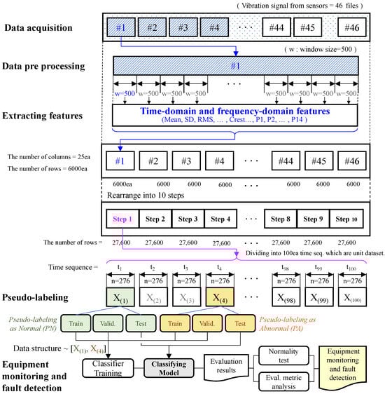
Figure 2.
The proposed procedure for equipment monitoring and fault detection.
4. Theoretical Background
4.1. Random Forest
In this section, we briefly review random forest. By combining multiple classifiers, RF estimates the final result by averaging or voting. It is derived from the bagging algorithm and the stochastic subspace method, which were both proposed by Leo Breiman in 2001 [34]. In 1984, Breiman and Stone introduced the CART (classification and regression tree) decision tree algorithm, which is the basic classifier for the RF algorithm. To select feature attributes, the algorithm uses the Gini index minimum criterion, as opposed to the ID3 decision tree algorithm and the C4.5 decision tree algorithm. In order to define the purity of the data set, D, we need to consider the following [7,35]:
The Gini index is defined as follows:
The RF algorithm follows a flow similar to the classic bagging algorithm:
- Bootstrap resampling is run k times on the original sample data set, thus collecting a fixed number of samples each time, taking them back out after each sampling, and then obtaining K subsample sets.
- The CART algorithm is used to generate a decision tree for each subsample set. If feature from the ith subsample set contains C categories, the Gini index is calculated as follows: In the case that the feature from the ith subsample set contains C categories, the Gini index is calculated as follows:where is the probability of category . As a result of Equation (3) below, a smaller Gini value indicates a higher level of purity. In the decision tree, the feature with the smallest Gini value is split.
- Based on Step 2, each subsample set generates a decision tree, and the decision trees of all the subsample sets form a random forest. Each decision tree is pruned according to the minimum Gini criterion by automatically selecting M features from feature set T containing M features as the attribute separation.
- A majority voting algorithm is used to analyze and vote on the results of the final RF algorithm.
4.2. Support Vector Machines
The SVM is a computational learning method that is based on the statistical learning theory developed by Vapnik in 1999. The SVM uses a high-dimensional dot product space called a feature space, which maps original input spaces onto a high-dimensional plane called a hyperplane, which is calculated to maximize the generalization capability of the classifier to maximize its accuracy. It is possible to find the maximal hyperplane using optimization theory and statistical learning theory as an approach that respects insights provided by the latter. In addition, SVMs are capable of handling very large feature spaces, since their training takes place in a manner such that the dimensions of a class vector do not have as high of an impact on the performance of the SVM as they do on the performance of a conventional classifier. As a result, the SVM is particularly effective in classification problems that involve a large number of variables. Furthermore, fault classification will be improved due to the fact that fault diagnosis need not be limited by the number of features a fault can possess. Additionally, SVM-based classifiers are typically trained so that the empirical risk or structural misclassification risk is minimized, whereas traditional classifiers are usually trained so that the structural risk is minimized [36].
Given the data input , M is the number of samples. In this case, there are two classes of samples: positive and negative. Each class is associated with labels for positive and for negative. A linear data set can be separated from the given data set by determining the hyperplane :
where w is the M-dimensional vector, and b is a scalar. It is defined by the scalar b and vector w where the separating hyperplane is located. By using , a decision function is created for classifying input data as positive and negative. It is necessary for a distinctly separated hyperplane to satisfy the following constraints:
or it can be presented in the complete equation:
The optimal separate hyperplane creates the maximum distance between the plane and the nearest data, i.e., the maximum margin. A solution to the following optimization problem can be obtained by considering the slack variable, , and the error penalty, C, in the noise:
where measures the distance between the margin and the examples that lie on the wrong side of the margin.
It is possible to apply SVMs to nonlinear classification tasks, as well using kernel functions. A high-dimensional feature space is used to map the data to be classified where linear classification is possible. A linear decision function is obtained in dual form by mapping the n-dimensional input vector x onto an l-dimensional feature space using the nonlinear vector function :
In high-dimensional feature spaces, complex functions can be expressed, but they also generate problems. Overfitting occurs because of the high dimensionality and the large vectors. Kernel functions can be used to solve the latter problem. is a function that returns the dot product of the feature space mappings of the original data points, which is defined as . In the feature space, it is not necessary to explicitly evaluate when applying a kernel function, and the decision function will be
linear kernels, polynomial kernels, and Gaussian kernels are some of the kernel functions used in SVMs. In order for the training set examples to be classified correctly, the kernel function must be chosen carefully. This paper evaluates and formulates radial, linear, sigmoid, and polynomial functions.
4.3. Model Performance Evaluation Metrics
In order to properly estimate their capabilities, it is crucial to thoroughly examine the diagnostic abilities of several machine learning algorithms while accounting for variables such as model complexity, computational needs, and parameterization. For this reason, it is necessary to use defined criteria for assessing performance and discriminating between candidates. The F1 score, accuracy, sensitivity, precision, and false alarm rate are among these parameters. With these measurements, we can objectively compare and assess the performance of various models, thus allowing us to make informed decisions based on their individual benefits and drawbacks [35,37]. These are some of the evaluation metrics that have been used in studies: Equations (11)–(14).
True positive (TP) indicates that the model accurately predicted a true outcome. False positive (FP) indicates the model predicted a true outcome, but the actual outcome was false. False negative (FN) indicates that the model’s predicted a false result, while the actual result was true. True negative (TN) indicates the model accurately predicted a false result. The accuracy of a model is often used to evaluate its performance, but accuracy has several drawbacks. In unbalanced data sets, one class is more common than the others, and the model will label observations based on this imbalance. If 90% of the cases are false and only 10% are true, there is a high possibility that the model would have an accuracy of around 90%. Precision is calculated as the number of true positives over the total number of positives predicted by the model. This metric allows you to calculate the rate at which your positive predictions actually come true. Sensitivity (also known as recall) is the percentage of actual positive outcomes compared to all true positive predictions. It is possible to evaluate how well our model predicts the true outcome. Specificity is a measure of how well predicted negatives turned out to be negative.
4.4. Feature Extraction
For ML algorithms to be able to extract essential information from complex data sets, feature extraction is an important step before training. It can be used to identify key patterns within the signals, as well as anomalies or outliers. By simplifying the data set, classification tasks can be carried out more efficiently [4]. The formulas for common statistical features that can be extracted from both the time domain and frequency domain are shown in Table 1 and Table 2. Whenever there is a fault in a mechanical system, the stiffness of the mechanical structures around the fault must change, thereby causing a shock or impulse to occur. Additionally, this may cause the vibration signals to vary. It is possible to change the amplitudes and distributions of these time domain signals. As a result, mechanical faults can be reflected in their time domain wave forms as time domain statistical features. As shown in Table 1, there are a number of common statistical features in the time domain. The mean value here represents the average of a signal. The root amplitude, root mean square, and peak of a time domain signal can be used to assess the vibration amplitude and energy. In general, mechanical vibration can cause the mean value, root amplitude, root mean square, and peak to rise when there is a fault. These four characteristics can be used to determine the severity of a fault as it becomes more severe. It is, however, not sensitive to weak, incipient faults. A time series distribution in the time domain may be represented using the skewness, kurtosis, crest factor, clearance factor, shape factor, and impulse factor. An impulse in vibration signals can be measured by the kurtosis value, the crest factor, the impulse factor, and the clearance factor. Kurtosis and crest factors can be used as indicators for incipient faults, because they are robust to varying operating conditions. Impulse and clearance factors are useful indicators of the sharpness of the impulses created by a defect contacting the bearing mating surfaces. The kurtosis value is highly sensitive to early faults. Kurtosis values can also increase gradually as the degree of severity increases. In contrast, they decrease unexpectedly when the fault is even more severe. Therefore, kurtosis is insufficient for measuring more severe faults. As shown in Table 1, different statistical features in the time domain can reflect mechanical health from different perspectives. They can compensate for each other. For different fault levels, each indicator contains different fault information. In some cases, even many indicators cannot accurately reflect the changes in faults. For this reason, it is necessary to extract more features from rotating machinery to efficiently diagnose faults, and sensitive features should also be screened out. The frequency spectra of vibration signals can reveal abnormal frequencies when there is a fault in machinery, which can reflect the machinery’s condition. In addition, frequency spectra are more sensitive to incipient faults, as an imperceptible change produces a spectrum line in diagnostics, which can be used to extract some spectral indicators. The frequency domain features may also contain information that is not present in the time domain, such as fault-related information. These features in the frequency domain compensate for those in the time domain alone. Table 2 shows 14 common statistical features in the frequency domain. All of them are based on statistics, so they are called statistical features. , the mean frequency, represents the average of the amplitudes of all the frequencies in the frequency domain. As fault degrees increase, the mean frequency must also increase. It may be that features , , , , and , , and reflect the convergence of the energy of the frequency spectrum. The position of the dominant frequencies in the frequency spectrum may be shown by features , , , and . Accordingly, these frequency domain features can be used to reflect mechanical health from a variety of perspectives. There will be vibrations across the entire frequency spectrum and power spectrum due to different faults. To achieve accurate diagnosis results, we need to select suitable statistical features based on the different fault categories [38]. The 11 time domain features of a vibration signal and the 14 frequency domain features were calculated separately for each signal. According to the specified procedure, all features were calculated sequentially for each batch: , a signal series for where N is the number of data points; , a spectrum for where K is the number of spectrum lines; and , the frequency value of the kth spectrum line.

Table 1.
Time domain statistical features.
Table 2.
Feature domain statistical features.
5. Experiment Validation
5.1. Data Acquisition and Preprocessing
In order to monitor gearbox abnormalities, the test rig was constructed using motors and gearboxes that are actually used in the field. A speed motor and torque motor were installed; gearbox 1 was operated at high speed, and gearbox 2 was operated at low speed. The specifications of the basic motor and gearbox are shown in Figure 3. The preprocessing, feature extraction, and pseudo labeling processes of the collected data are shown in Figure 2 in Section 3. We set 500 ea of the raw data as one window size, extracted features in the time domain and frequency domain, divided them into 10 steps, and saved them. At this time, each step had 27,600 ea of data, and a pseudolabel was given every 276 ea. The 276 ea dataset was divided into a train, test, and valid set. This data was used to train the classifer [39].
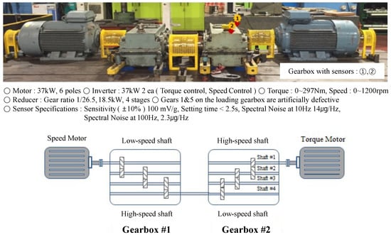
Figure 3.
Gearbox test bench scheme.
5.2. Experiment Results
Figure 4 shows how the classification accuracy changed with time for each step. The black triangles on the graphs indicate changes in the LM’s classification accuracy. In Step 1, the classification accuracy started at 0.5 and gradually increased, thus reaching 0.9 around time sequence 65. The results are caused by the naturally increased vibration as the rotation speed of the motor connected to the gearbox increases. The LM has two limitations: it generates false alarms from normal changes, and it is difficult to detect changes in the equipment status when smaller changes are accumulating. Classification accuracy values by the proposed Reduced Lagrange Method are shown in blue (DS) and magenta (NDS). The proposed R-LM showed classification accuracy values of around 0.5 up to time sequence 60, but the accuracy began to increase only at the point at which the equipment status was estimated to have changed. The LM can be used to identify changes in the status of equipment over time when a specific set of data can be maintained with confidence in a steady state. However, the proposed R-LM responds sensitively to changes within the predesigned round size interval (k). It is possible to check this in Steps 3 and 4. While the LM’s classification accuracy value increased gently over time, the proposed R-LM had a constant value around 0.5. Steps 6 and 7 did not show meaningful changes in the equipment status from either the LM or the proposed R-LM. There was a catastrophic failure in Step 8. The LM showed a rapid change in equipment status starting at time sequence 50, which indicated an increase in classification accuracy. The proposed R-LM also showed rapid changes in equipment status at time sequence 50 and at two peaks. When the equipment status changed and remained there, the classification accuracy values from the R-LM were low. This is characteristic of the R-LM, which only responds when equipment conditions change. The analysis of the vibration signal on the nondrive side showed high classification accuracy in time sequences 1 to 10 of Step 8. That means that abnormal signals can be generated before catastrophic failures occur in the equipment. False alarms may cause field maintenance workers to lose confidence in the equipment monitoring system, so minimizing false alarms is important. Pseudolabeling provides limited information for fault detection and diagnosis, because it does not accurately match normal and abnormal field labels. If event data generated from equipment operation and maintenance are analyzed with false alarms, they can be reduced. Maintenance resources can be utilized more efficiently by reducing false alarms. In Table 3, changes are shown in the accuracy, precision, specificity, and sensitivity. One value is the average of the top five ranked values of 100 evaluation metrics. When it exceeds 0.7, an alarm occurs, and if it exceeds 0.95, a warning occurs. In Step 4, the LM generated false alarms with increasing classification accuracy, but the proposed R-LM remained within a classification accuracy of 0.5.
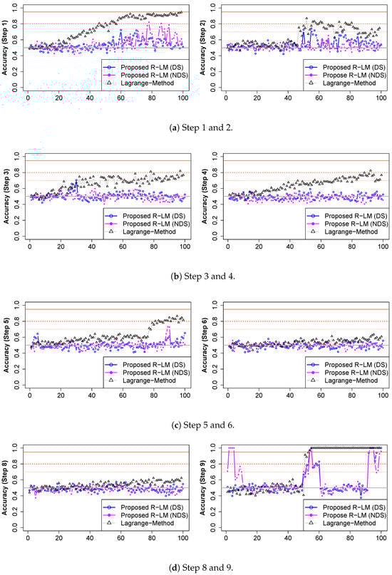
Figure 4.
(a–d) The evaluation metric step by step.
Table 3.
The evaluation metric results by kernel.
5.3. Normality Test for Classification Evaluation Metrics
Based on classification accuracy data, it can be determined that the vibration data acquired during this time were derived from a homogeneous sample. That means that there were no significant changes to the equipment. In Figure 5, we can see that the classification accuracy data for Steps 1, 2, 3, 9, and 10 are not normally distributed. We performed a hypothesis test for normality to quantitatively confirm this. Table 4 shows that the steps with a p value of 0.05 or less are Steps 1, 2, 3, 9, and 10 for the drive side and Steps 1, 2, 3, 5, 9, and 10 for the nondrive side. Since a catastrophic failure occurred in Step 9, it confirmed that signs of equipment abnormalities had already appeared in Steps 1, 2, and 3. As a result, the normality test result for the classification accuracy values obtained by assigning a pseudolabel to the data set and applying the Reduced Lagrange Method can be classified as abnormal (A) if the p value is less than 0.05, and the result can be classified as normal if the p value is greater than 0.05. An alarm signal can thus be generated when the status of the equipment changes.
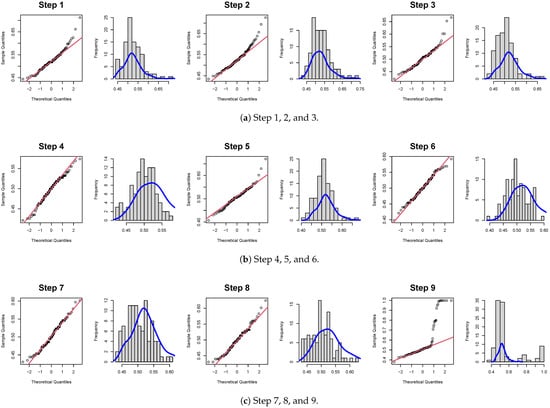
Figure 5.
(a–c) The Q–Q plot and histogram of classification accuracy.
Table 4.
Normality test results (p values).
5.4. Variable Importance and Partial Dependence Plot
In binary classification, frequency domain features have a more significant role than time domain features. The frequency domain features ranked relatively high and were selected as important features in the variable importance analysis. Through partial dependency analysis, we can confirm the direction of change, as well as the influence of the variables. A partial dependence plot (PDP) in the time domain is shown in Figure 6 and Figure 7. A PDP represents how features affect the target variable of the prediction model. The x axis and the y axis represent the feature value and predicted abnormality, respectively. Features , , , , , and were rarely considered abnormal, even when they increased in value. There are some features that are not related to the target variables even if their values change. Skewness, kurtosis, crest, shape, impulse, and , , and are representative examples. Figure 6a,b show the partial dependence analysis results for each feature extracted from the NDS. Upon analyzing the features extracted from the vibration signal on the nondrive side, SD, root, RMS, skewness, and and , the target variable was judged to be abnormal as the feature value increased. When the feature value became smaller, , , , , , and tended to be considered normal. There are some features that do not have a meaningful relationship with the target variable, no matter how their values changed. The mean, peak, kurtosis, crest, shape, and impulse, plus , , , and are examples. Alarms are generated in the field when the vibration average value (a time domain feature) exceeds a set value. Time domain features are used in the field to generate alarms, but they have limitations. A frequency domain feature can therefore be used to predict equipment status changes more accurately than a time domain feature. Data analysis in the frequency domain is essential, along with data analysis in the time domain.
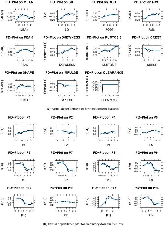
Figure 6.
(a,b) Partial dependence plot (NDS). Black line: Partial dependence value. Blue line: flattened trend value.
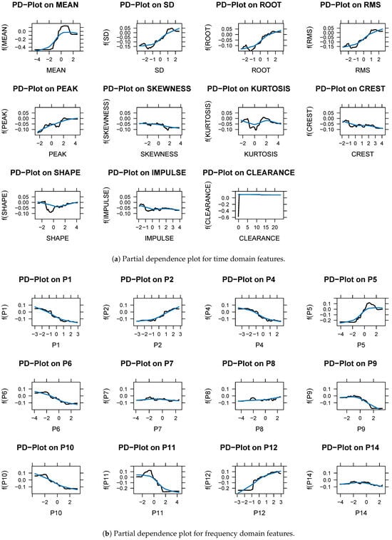
Figure 7.
(a,b) Partial dependence plot (DS). Black line: Partial dependence value. Blue line: flattened trend value.
6. Discussion and Conclusions
A new era of data-driven fault detection and monitoring is emerging in the Industry 4.0 age as computing power, the IoT, and big data technologies grow rapidly. A gearbox is one of the key components used in rotating machinery, along with bearings. An unplanned shutdown of equipment will negatively affect production, quality, cost, and the delivery date, as well as safety and the environment. In order to prevent equipment failure, it is crucial to monitor the equipment’s condition and predict it in advance. In most studies, failure types were created in advance and analyzed in the lab. This means that laboratory results will not be as good as field results if they are applied directly to analysis in the field. Due to the lack of labels in the field, the proposed methodology has limitations in application and analysis. Currently, a condition monitoring system collects vibration signals and issues an alarm when the vibration signal exceeds a preset value. Field workers have little confidence in monitoring systems in this situation, since false alarms are frequently caused by changes in vibration due to regular operations and periodic equipment repairs. This paper demonstrated how pseudolabeling techniques can be applied to unlabeled data and used to monitor changes in equipment conditions. The proposed method makes the following contributions. First of all, false alarms can be reduced compared to existing methods. The classification accuracy value was used to identify the point at which the equipment condition changed. By linking this information to meta data, false alarms can be further reduced, thereby increasing the reliability of the monitoring system and reducing maintenance costs. A normality hypothesis test was used to quantitatively determine whether the equipment status had changed, and its effectiveness was confirmed. Finally, the relationship between the explanatory variable and the target variable was confirmed when the explanatory variable changed. By using this method, we were able to compensate for the limitations of machine learning, which has excellent prediction results without explaining why such results are obtained. In this study, data indicating abnormalities were collected without labels from field equipment and were used as input. We proposed a method and procedure for assigning pseudolabels to the collected data to monitor changes in the equipment status using a supervised learning classifier. The main goal of an actual gearbox inspection is to detect and prevent unexpected failures by carefully inspecting equipment where its condition changes rapidly or continuously. Through accumulated data, we were able to predict equipment status and prevent sudden breakdowns. Therefore, by establishing a cost-effective maintenance plan, we can expect industry to become more competitive. In the future, it will be important to investigate how to determine the number of k classifier operations within a round.
In the future, equipment condition monitoring and diagnostic performance will be able to be improved through the following studies:
- It is still necessary to find the optimal combination of hyper parameters used in pseudolabel analysis, such as the interval between normal and abnormal data sets (d), the data set window size (w), and the movement interval (s).
- There is a need for research on a hybrid LM, which monitors equipment conditions with R-LM under normal conditions and switches to LM under abnormal conditiosn to monitor accumulated changes. The advantages of R-LM and LM will be combined if a hybrid LM is successfully developed.
- Research that predicts equipment condition changes and categorizes them according to their type can reduce false alarms and contribute to the diagnosis of equipment problems.
Author Contributions
Conceptualization, M.-K.S. and W.-Y.Y.; methodology, M.-K.S. and W.-Y.Y.; software, M.-K.S.; formal analysis, M.-K.S.; investigation, M.-K.S.; resources, M.-K.S.; data curation, M.-K.S.; writing—original draft, M.-K.S. and W.-Y.Y.; writing—review and editing, W.-Y.Y.; visualization, M.-K.S.; supervision, W.-Y.Y.; project administration, W.-Y.Y. All authors have read and agreed to the published version of the manuscript.
Funding
This research received no external funding.
Data Availability Statement
The data presented in this study are available upon request from the corresponding author. The data are not publicly available due to laboratory regulations.
Conflicts of Interest
Author Myung-Kyo Seo was employed by the company POSCO (Pohang Iron and Steel Co., Ltd. The remaining authors declare that the research was conducted in the absence of any commercial or financial relationships that could be construed as a potential conflict of interest.
Abbreviations
The following abbreviations are used in this manuscript:
| AE | Autoencoder |
| AI | Artificial Intelligence |
| BM | Breakdown Maintenance |
| CART | Classification and Regression Tree |
| CBM | Condition-Based Maintenance |
| CNN | Convolutional Neural Networks |
| DS | Drive Side |
| FDD | Fault Detection and Diagnosis |
| GPUs | Graphics Processing Units |
| LM | Lagrange Method |
| ML | Machine Learning |
| NDS | Nondrive Side |
| PDP | Partial Dependence Plot |
| R-LM | Reduced Lagrange Method |
| RF | Random Forest |
| PM | Preventive Maintenance |
| SVM | Support Vector Machine |
References
- Yacout, S. Fault detection and Diagnosis for Condition Based Maintenance Using the Logical Analysis of Data. In Proceedings of the 40th International Conference on Computers and Industrial Engineering Computers and Industrial Engineering (CIE), Awaji, Japan, 25–28 July 2010; pp. 1–6. [Google Scholar]
- Farina, M.; Osto, E.; Perizzato, A.; Piroddi, L.; Scattolini, R. Fault detection and isolation of bearings in a drive reducer of a hot steel rolling mill. Control Eng. Pract. 2015, 39, 35–44. [Google Scholar] [CrossRef]
- Niu, G. Data-Driven Technology for Engineering Systems Health Management: Design Approach, Feature Construction, Fault Diagnosis, Prognosis, Fusion and Decisions; Springer: Berlin/Heidelberg, Germany, 2017. [Google Scholar]
- Kumar, S.; Goyal, D.; Dang, R.K.; Dhami, S.S.; Pabla, B.S. Condition based maintenance of bearings and gears for fault detection—A review. Mater. Today Proc. 2018, 5, 6128–6137. [Google Scholar] [CrossRef]
- Lei, Y.; Zuo, M.J. Gear crack level identification based on weighted K nearest neighbor classification. Mech. Sys. Siganl Process. 2009, 23, 1535–1547. [Google Scholar] [CrossRef]
- Fan, S.; Cai, Y.; Zhang, Z.; Wang, J.; Shi, Y.; Li, X. Adaptive Convolution Sparse Filtering Method for the Fault Diagnosis of an Engine Timing Gearbox. Sensors 2023, 24, 169. [Google Scholar] [CrossRef]
- Tang, X.H.; Gu, X.; Rao, L.; Lu, J.G. A single fault detection method of gearbox based on random forest hybrid classifier and improved Dempster-Shafer information fusion. Comput. Electr. Eng. 2021, 92, 107101. [Google Scholar] [CrossRef]
- Chen, Z.; Li, C.; Sanchez, R.V. Gearbox fault identification and classification with convolutional neural networks. Shock. Vib. 2015, 2015, 390134. [Google Scholar] [CrossRef]
- Jing, L.; Zhao, M.; Li, P.; Xu, X. A CNN based feature learning and fault diagnosis method for the condition monitoring of gearbox. Measurement 2017, 111, 1–10. [Google Scholar] [CrossRef]
- Lee, J.H.; Okwuosa, C.N.; Hur, J.W. Extruder Machine Gear Fault Detection Using Autoencoder LSTM via Sensor Fusion Approach. Inventions 2023, 8, 140. [Google Scholar] [CrossRef]
- Ramteke, D.S.; Parey, A.; Pachori, R.G. A New Automated Classification Framework for Gear Fault Diagnosis Using Fourier–Bessel Domain-Based Empirical Wavelet Transform. Machines 2023, 11, 1055. [Google Scholar] [CrossRef]
- Lupea, L.; Lupea, M. Detecting Helical Gearbox Defects from Raw Vibration Signal Using Convolutional Neural Networks. Sensors 2023, 23, 8769. [Google Scholar] [CrossRef] [PubMed]
- Hu, P.; Zhao, C.; Huang, J.; Song, T. Intelligent and Small Samples Gear Fault Detection Based on Wavelet Analysis and Improved CNN. Processes 2023, 11, 2969. [Google Scholar] [CrossRef]
- Tran, V.T.; Yang, B.S. An intelligent condition-based maintenance platform for rotating machinery. Expret Syst. Appl. 2012, 39, 2977–2988. [Google Scholar] [CrossRef]
- Lee, S.H.; Youn, B.D. Industry 4.0 and direction of failure prediction and health management technology (PHM). J. Korean Soc. Noise Vib. Eng. 2015, 21, 22–28. [Google Scholar]
- Pecht, M.G.; Kang, M.S. Prognostics and Health Management of Electronics-Fundamentals Machine Learning, and the Internet of Things; John Wiley and Sons: Hoboken, NJ, USA, 2008. [Google Scholar]
- Choi, J.H. A review on prognostics and health management and its application. J. Aerosp. Syst. Eng. 2014, 38, 7–17. [Google Scholar]
- Yang, B.S.; Widodo, A. Introduction of Intelligent Machine Fault Diagnosis and Prognosis; Nova: Dongtan, Republic of Korea, 2009. [Google Scholar]
- Widodo, A.; Yang, B.-S. Support vector machine in machine condition monitoring and fault diagnosis. Mech. Syst. Signal Process 2007, 21, 2560–2574. [Google Scholar] [CrossRef]
- Banerjee, T.P.; Das, S. Multi-sensor data fusion using support vector machine for motor fault detection. Inf. Sci. 2012, 217, 96–107. [Google Scholar] [CrossRef]
- Park, J.; Kwon, I.H.; Kim, S.S.; Baek, J.G. Spline regression based feature extraction for semiconductor process fault detection using support vector machine. Expert Syst. Appl. 2011, 38, 5711–5718. [Google Scholar] [CrossRef]
- Wang, C.C.; Wu, T.Y.; Wu, C.W.; Wu, S.D. Multi-Scale Analysis Based Ball Bearing Defect Diagnostics Using Mahalanobis Distance and Support Vector Machine. Entropy 2013, 15, 416–433. [Google Scholar]
- Shin, I.S.; Lee, J.M.; Lee, J.Y.; Jung, K.S.; Kwon, D.I.; Youn, B.D.; Jang, H.S.; Choi, J.H. A Framework for prognostics and health management applications toward smart manufacturing system. Inter. J. Precis. Eng. Manuf.-Green Tech. 2018, 5, 535–554. [Google Scholar] [CrossRef]
- Hadi, R.H.; Hady, H.N.; Hasan, A.M.; Al-Jodah, A.; Humaidi, A.J. Improved Fault Classification for Predictive Maintenance in Industrial IoT Based on AutoML: A Case Study of Ball-Bearing Faults. Processes 2023, 11, 1507. [Google Scholar] [CrossRef]
- Santamaria-Bonfil, G.; Arroyo-Figueroa, G.; Zuniga-Garcia, M.A.; Ramos, C.G.A.; Bassam, A. Power Transformer Fault detection: A Comparision of Standard Machine Learning and autoML Approach. Energies 2023, 17, 77. [Google Scholar] [CrossRef]
- Brescia, E.; Vergallo, P.; Serafino, P.; Tipaldi, M.; Cascella, D.; Cascella, G.L.; Romano, F.; Polichetti, A. Online Condtion Monitoring of Industrial Loads Using AutoGMM and Decision Tree. Machines 2023, 11, 1082. [Google Scholar] [CrossRef]
- Hong, S.; Lu, Y.; Dunning, R.; Ahn, S.H.; Wang, Y. 2012 Adaptive fusion based on physics-constrained dictionary learning for fault diagnosis of rotating machinery. Manuf. Lett. 2023, 35, 999–1008. [Google Scholar] [CrossRef]
- Lu, Y.; Wang, Y. A physics-constrained dictionary learning approach for compression of vibration signals. Mech. Syst. Signal Process. 2021, 153, 107434. [Google Scholar] [CrossRef]
- Miao, M.; Sun, Y.; Yu, J. Sparse representation convolutional autoencoder for feature learning of vibration signals and its applications in machinery fault diagnosis. IEEE Trans. Ind. Electron. 2021, 69, 13565–13575. [Google Scholar] [CrossRef]
- Seo, M.-K.; Yun, W.-Y. Clustering-based monitoring and fault detection in hot strip rolling mill. J. Korean Soc. Qual. Manag. 2017, 45, 298–307. [Google Scholar] [CrossRef]
- Seo, M.-K.; Yun, W.-Y. Clustering-based hot strip rolling mill diagnosis using Mahalanobis distance. J. Korean Inst. Ind. Eng. 2017, 43, 298–307. [Google Scholar]
- Seo, M.-K.; Yun, W.-Y. Condition Monitoring and Diagnosis of a Hot Strip Roughing Mill Using an Autoencoder. J. Korean Soc. Qual. Manag. 2019, 47, 75–86. [Google Scholar]
- Seo, M.-K.; Yun, W.-Y.; Seo, S.-K. Machine Learning Based Equipment Monitoring and Diagnosis Using Pseudo-Label Method. J. Korean Inst. Ind. Eng. 2020, 46, 517–526. [Google Scholar]
- Breiman, L.; Friedman, J.H.; Olshen, R.A.; Stone, C.J. Classification And Regression Trees; Chapman & Hall/CRC: Boca Raton, FL, USA, 1984. [Google Scholar]
- Yaqub, R.; Ali, H.; Wahab, M.H.B.A. Electrical Motor Fault Detection System using AI’s Random Forest Classifier Technique. In Proceedings of the 2023 IEEE International Conference on Advanced Systems and Emergent Technologies, Hammamet, Tunisia, 29 April–1 May 2023. [Google Scholar]
- Niu, G. Data-Driven Technology for Engineering Systems Health Management; Science Press, Springer: Beijing, China, 2017. [Google Scholar]
- Zhong, J.; Yang, Z.; Wong, S.F. Machine Condition Monitoring and Fault Diagnosis based on Support Vector Machine. In Proceedings of the 2010 IEEE International Conference on Industrial Engineering and Engineering Management, Macao, China, 7–10 December 2010. [Google Scholar]
- Lei, Y. Intelligent Fault Diagnosis and Remaining Useful Life Prediction of Rotating Machinery; Butterworth-Heinemann: Oxford, UK, 2016. [Google Scholar]
- Seo, M.-K.; Yun, W.-Y. Hot Strip Mill Gearbox Monitoring and Diagnosis Based on Convolutional Neural Networks Using the Pseudo-Labeling Method. Appl. Sci. 2024, 14, 450. [Google Scholar] [CrossRef]


Disclaimer/Publisher’s Note: The statements, opinions and data contained in all publications are solely those of the individual author(s) and contributor(s) and not of MDPI and/or the editor(s). MDPI and/or the editor(s) disclaim responsibility for any injury to people or property resulting from any ideas, methods, instructions or products referred to in the content. |
© 2024 by the authors. Licensee MDPI, Basel, Switzerland. This article is an open access article distributed under the terms and conditions of the Creative Commons Attribution (CC BY) license (https://creativecommons.org/licenses/by/4.0/).