A Unified Approach to Modeling and Simulation of Underwater Vehicle Multi-Manipulator Systems

Abstract

In this article, the model of a family of underwater vehicle multi-manipulator systems (UVMMS) is obtained by considering all its elements as parts of a unique system, the model includes the forces produced on the manipulators by the movement of the vehicle, as well as the reaction forces on the vehicle produced by the movement of the manipulators. The modeling process is completed using the Newton–Euler approach through the mobile arborescent kinematic chain. This work also presents different approaches to the use of numerical implementations of the proposed model, and simulation results are included to demonstrate that the model is capable to represent the interaction between the vehicle and the manipulators. The proposed model and simulations are important because they allow the design of control strategies that consider all the elements of the system instead of neglecting the interaction forces or considering the vehicle and the arms as uncoupled elements.

1. Introduction

The incursion of drones has increased due to the need for spatial and temporal data coverage of specific areas where human intervention is risky, such as disaster areas, high-risk environments due to viral or radioactive contamination, and difficult-to-access areas due to great depths or heights. Drones are small mobile robots (3–20 kg) that can be terrestrial, aerial, and submarine.

In the last five years, Unmanned Underwater Drones (UUD) have become a standard tool for researching marine life, some examples of which include the monitoring, tracking, and imaging of a randomly moving shark [1] and the study of a school of fish in an altered environment, as carried out in the tropical reservoir (oligo-mesotrophic and warm monomictic) located in southeastern Brazil [2]. However, although underwater drones are a valuable tool for data collection and are becoming less expensive, they still have limitations due to possible equipment effects, such as different light intensities and the artificial noise, speed, size, and depth of the vehicle, resulting in the alteration of the behavior of the species to be studied.

In addition to marine life, shipwreck hulls and vestiges of war can also be found in the sea. Among these inorganic wastes, some that are considered marine litter include historical pieces or hazardous material. Every year, it is estimated that 5.1 million tons of mismanaged plastic enter the oceans worldwide. 75% of marine litter (ML) goes to beaches while the rest remains in seawater [3]. This problem is an area of opportunity for collaboration between an aerial drone and an underwater drone, as presented in [4], to acquire information on the progress and dimension of marine litter using the aerial drone while with the underwater drone, it is possible to obtain specifications of this garbage, such as the type of material and level of contamination in the water, reducing the costs of hiring planes, boats or divers.

Marine archaeology is an area of research that aims to rescue historical finds from the depths. For example, in [5], a study with an underwater drone of a shipwreck from the fourth-century B.C. near the island of Chios, Greece, was carried out, obtaining qualitative and quantitative data documenting the condition of the ancient shipwreck. In the case of war material found on the seabed, a proposal is presented in [6] to analyze the danger of this material through the BASTA project (Boost Applied ammunition detection through Smart data inTegration and AI workflows), tasked with identifying and improving underwater unexploded ordnance (UXO) detection approaches.

The UUDs can be equipped with a robotic arm to perform more complex tasks, obtaining an Underwater Vehicle Manipulation System (UVMS). Some tasks a UVMS executes are the collection of objects [7] and marine products [8] and the maintenance of underwater structures [9], among others. Depending on the degrees of freedom of the manipulator robot to be coupled to the underwater drone, it will be challenging to carry out the assigned task for the UVMS due to the disturbances added to the drone caused by the movement of the manipulator.

When a UVMS has more than one manipulator robot attached to its mobile platform, the result is an underwater vehicle multi-manipulator system (UVMMS). Although some bio-inspired underwater robots known as bionics possess mechatronic multibodies, they differ from a UVMMS due to motion generation, as can be reviewed in [10,11].

The aggregated disturbances or interaction forces in a UVMS can be estimated by generating a mathematical model, which is acquired through different methodologies, depending on the researcher’s focus. Suppose the UVMS is analyzed as two independent systems. In that case, the UUD as vehicle is model with the methodology reported in [12], where a movement of 6-DOF in an underwater environment with external forces is considered. The external component depends on the fluid, represented by the Euler–Lagrange technique. At the same time, the manipulator robot can define it using the Newton–Euler or Euler–Lagrange formulism.

Suppose it is desired to obtain the mathematical model as a coupled and unique system. In that case, there are some techniques presented in the literature, such as [13] where the system is expressed as the sum of two forces, generalized active force and generalized inertia force, obtained from the analysis of linear and angular speeds and accelerations; while in [14], the modeling strategy is derived from the Newton–Euler formulation, taking the base of the manipulator as a mobile base. However, the mentioned methodologies lack information to reproduce the technique.

This article presents a model of a UVMMS represented as a dependent system between its elements, that is, where the manipulator robot depends on the movement information of the underwater vehicle, and in turn, the underwater vehicle requires information about the torques generated due to the movement of the vehicle. This reaction also depends on the disturbances of the marine environment.

The contribution of this paper is to extend the dynamic model for marine vehicles, described by Fossen [15], to the case of a particular family of UVMMS. A new notation is proposed to include the description of the vehicle as well as the manipulators in an intuitive way.

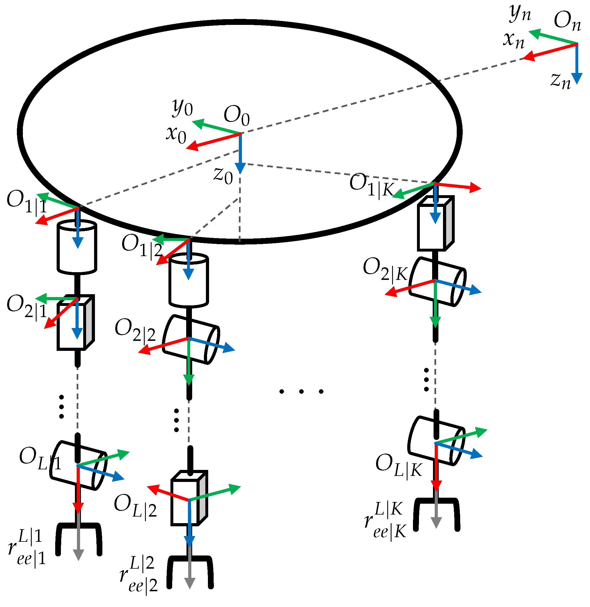
In the proposed analysis, the UVMMS consists of a 6-DOF (degree of freedom) underwater vehicle with K serial robotic manipulators with actuated joints. Figure 1 shows a scheme of the general system, where coordinate systems are represented using Red, Green and Blue color convention for the X, Y and Z axes. This color code will continue to be used in later sections to indicate axes in free-body diagrams.

The suggested approach for calculating the mathematical model is separated into three phases: kinematic, kinetic, and external forces analyses. For each phase, the study will be carried out for the general case and then applied to the vehicle and the manipulator links. The modeling technique used to analyze this system is the Newton–Euler formulation.

2. Kinematics

Kinematics refers to the study of motion without considering the forces that cause it. A kinematic model [16] includes a description of position r, angular velocity $\omega$, linear velocity v, angular acceleration $\alpha$, and linear acceleration a.

The system shown in Figure 1 has a complex geometric structure; to describe the kinematics of each one of its elements, it is necessary to fix frames in several parts of the system. In the proposed analysis, frames are located at the beginning of each link [17].

The origin of the inertial frame of the world is denoted by $O_n$ using the NED convention, the frame attached to the vehicle is represented by $O_0$, the location of the center of gravity (CoG) of the vehicle is denoted by $g_0$.

The origin of the frame attached to link l, of manipulator k, is denoted by $O_{l|k}$ and is defined using Denavit–Hartenverg convention (D-H), the attachment point of manipulator k is located at $O_{1|k}$, the location of the CoG of link l of manipulator k is denoted by $g_{l|k}$.

The total number of links of manipulator k is denoted by $L|k$, and the end effector’s location is indicated by $r_{ee/L|k}^{L|k}$.

Notation for rotations will be defined as $R_j^i$, which denotes the rotation matrix of origin $O_j$ relative to $O_i$.

Explicit notation for positions, velocities, and accelerations will be defined using two subscripts $j/i$, indicating the related frames, and one superscript k showing the frame used to express the quantity, i.e., $r_{j/i}^k$ denotes the relative position of origin $O_j$ relative to frame $O_i$ expressed in frame $O_k$.

A simplified notation will be defined to improve readability: the latter subscript will be omitted when it refers to the inertial frame, and the superscript will be omitted when it relates to the local frame, i.e., velocity $v_{l/n}^l$ denoted using explicit notation is equivalent to $v_l$ in simplified notation.

When considering moving frames, the derivative of a vector concerning time, depends on the frame chosen to perform the calculation. The notation for derivatives will be defined using a left subscript indicating the selected frame, i.e., $\frac{{}^{\mathit{n}}\mathit{d}}{dt}\left(v_{l/n}^n\right)$ represents the derivative of $v_{l/n}^n$ in the inertial frame.

Note that, in general, the derivative of a vector in the inertial frame $\frac{{}^{\mathit{n}}\mathit{d}}{dt}\left(v_{l/n}^n\right)$ is different from the derivative of the vector in the local frame $\frac{{}^{\mathit{l}}\mathit{d}}{dt}\left(v_{l/n}^l\right)$; the relation between these two concepts is obtained from the relation of the vectors to be derived $v_{l/n}^n=R_l^n{v}_{l/n}^l$, as follows in Equation (1):

$$\begin{array}{cc}\hfill \frac{{}^{\mathit{n}}\mathit{d}}{dt}\left(v_{l/n}^n\right)& =\frac{{}^{\mathit{n}}\mathit{d}}{dt}\left(R_l^n{v}_{l/n}^l\right)\hfill \\ \hfill & =R_l^n\frac{{}^{\mathit{l}}\mathit{d}}{dt}\left(v_{l/n}^l\right)+{\omega }_{l/n}^n\times R_l^n{v}_{l/n}^l\hfill \\ \hfill & =R_l^n\frac{{}^{\mathit{l}}\mathit{d}}{dt}\left(v_{l/n}^l\right)+{\omega }_{l/n}^n\times v_{l/n}^n\hfill \end{array}$$

(1)

This is obtained using the product rule for derivation and the fact that the derivative of a rotation matrix can be expressed in terms of a skew matrix of the corresponding angular velocity, which can be written in product form.

To avoid confusion, Newton’s notation will be used to denote derivative in local frame ${\dot{v}}_{l/n}^l=\frac{{}^{\mathit{l}}\mathit{d}}{dt}\left(v_{l/n}^l\right)$.

2.1. General Motion between Two Moving Frames

Consider a frame $O_j$ that is translating and rotating relative to frame $O_i$, which is also translating and rotating relative to inertial frame $O_n$, as shown in Figure 2. In this subsection, the general motion of frame $O_j$ is calculated, the equations found will be used to define the motion of the UVMMS links.

Although the next analysis is well known, there are several variations in the considerations and notation used in different areas, i.e., underwater vehicles and robotic manipulators, furthermore, particular movements are sometimes considered rather than the more general case, i.e., one of the frames is fixed or rotates but does not translate, etc. To avoid confusion with the existing literature, the angular and linear motion, to be used in the analysis of all elements of the UVMMS, is formulated here with the chosen notation.

2.1.1. Angular Motion

Orientation of frame $O_j$ relative to $O_n$, denoted by rotation matrix $R_j^n$, is calculated as the result of the successive rotations $R_i^n$ and $R_j^i$, as follows in Equation (2):

$$R_j^n=R_i^n{R}_j^i$$

(2)

Angular velocity of frame $O_j$ relative to $O_n$, denoted by ${\omega }_{j/n}^n$, is calculated by the derivative of Equation (2), which lends to Equation (3):

$${\omega }_{j/n}^n={\omega }_{i/n}^n+R_i^n{\omega }_{j/i}^i$$

(3)

Angular acceleration of frame $O_j$ relative to $O_n$, defined as ${\alpha }_{j/n}^n:=\frac{{}^{\mathit{n}}\mathit{d}}{dt}\left({\omega }_{j/n}^n\right)$, is calculated in Equation (4):    

$${\alpha }_{j/n}^n={\alpha }_{i/n}^n+R_i^n{\dot{\omega }}_{j/i}^i+{\omega }_{i/n}^n\times R_i^n{\omega }_{j/i}^i$$

(4)

2.1.2. Linear Motion

Position of frame $O_j$ relative to $O_n$, denoted by vector $r_{j/n}^n$, is the sum of positions $r_{i/n}^n$ and $r_{j/i}^n$, as follows in Equation (5):

$$r_{j/n}^n=r_{i/n}^n+R_i^n{r}_{j/i}^i$$

(5)

where relative position was calculated as $r_{j/i}^n=R_i^n{r}_{j/i}^i$.

Linear velocity of frame $O_j$ relative to $O_n$, defined as $v_{j/n}^n:=\frac{{}^{\mathit{n}}\mathit{d}}{dt}\left(r_{j/n}^n\right)$, is calculated as follows in Equation (6):

$$v_{j/n}^n=v_{i/n}^n+R_i^n{v}_{j/i}^i+{\omega }_{i/n}^n\times R_i^n{r}_{j/i}^i$$

(6)

Linear acceleration of frame $O_j$ relative to $O_n$, defined as $a_{j/n}^n:=\frac{{}^{\mathit{n}}\mathit{d}}{dt}\left(v_{j/n}^n\right)$, is calculated as follows in Equation (7):

$$a_{j/n}^n=a_{i/n}^n+R_i^n{\dot{v}}_{j/i}^i+{\alpha }_{i/n}^n\times R_i^n{r}_{j/i}^i+{\omega }_{i/n}^n\times (2R_i^n{v}_{j/i}^i+{\omega }_{i/n}^n\times R_i^n{r}_{j/i}^i)$$

(7)

The pose of $O_j$ defined using Equations (2) and (5) can be described, using simplified notation, as follows in Equation (8):

$$\begin{array}{cc}\hfill R_j^n& =R_i^n{R}_j^i\hfill \end{array}$$

(8a)

$$\begin{array}{cc}\hfill r_j^n& =r_i^n+R_i^n{r}_{j/i}^i\hfill \end{array}$$

(8b)

Velocity Equations (3) and (6) can be expressed in local frame by multiplying them by $R_n^j$, in simplified notation, as follows in Equation (9):

$$\begin{array}{cc}\hfill {\omega }_j& =R_i^j({\omega }_i+{\omega }_{j/i}^i)\hfill \end{array}$$

(9a)

$$\begin{array}{cc}\hfill v_j& =R_i^j(v_i+v_{j/i}^i+{\omega }_i\times r_{j/i}^i)\hfill \end{array}$$

(9b)

Acceleration Equations (4) and (7) can be expressed in local frame by multiplying them by $R_n^j$, in simplified notation, as follows in Equation (10):

$$\begin{array}{cc}\hfill {\alpha }_j& =R_i^j({\alpha }_i+{\dot{\omega }}_{j/i}^i+{\omega }_i\times {\omega }_{j/i}^i)\hfill \end{array}$$

(10a)

$$\begin{array}{cc}\hfill a_j& =R_i^j(a_i+{\dot{v}}_{j/i}^i+{\alpha }_i\times r_{j/i}^i+{\omega }_i\times (2v_{j/i}^i+{\omega }_i\times r_{j/i}^i))\hfill \end{array}$$

(10b)

2.2. Movement of the Vehicle

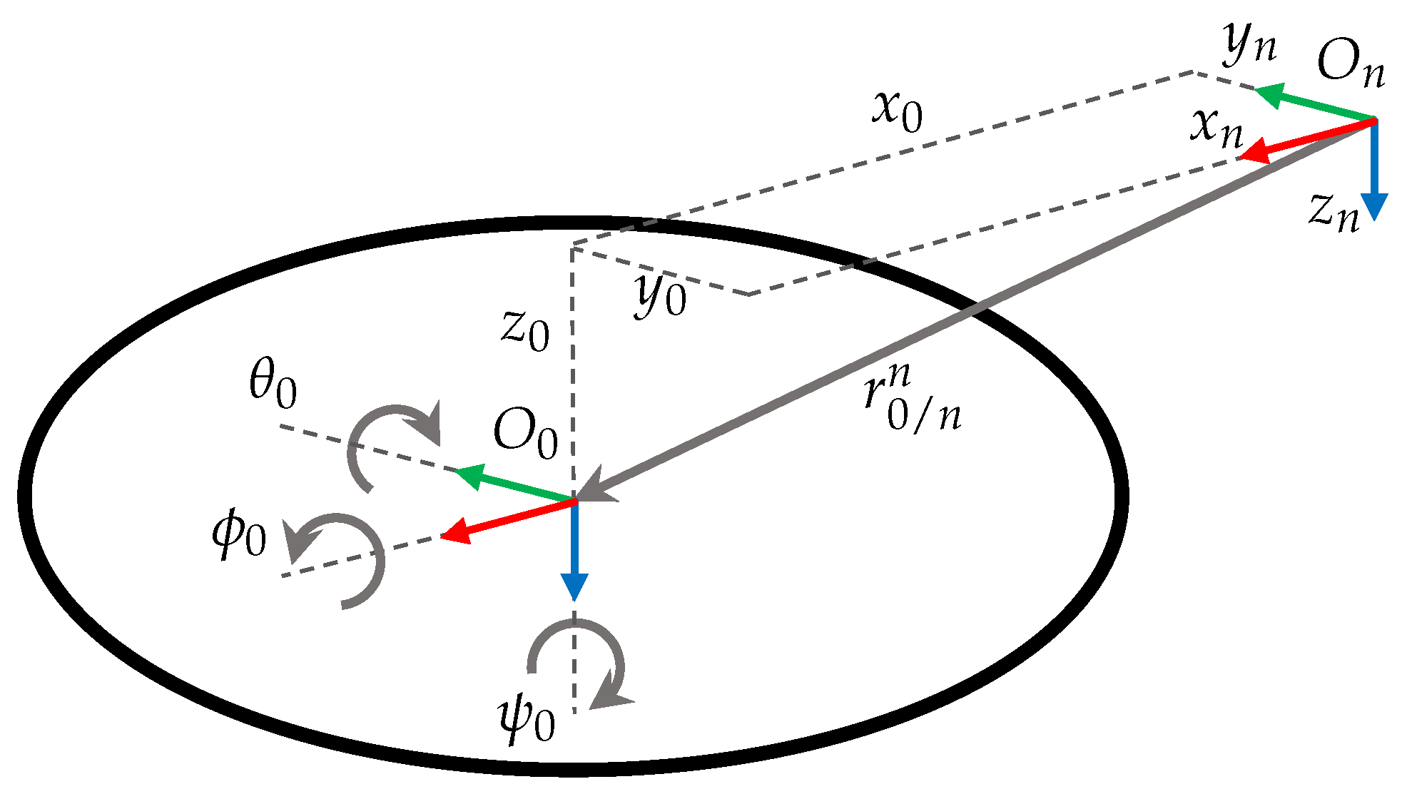
In this analysis, a 6-DOF underwater vehicle is considered: its position is defined using Cartesian coordinates, and its orientation is defined by a rotation matrix, relative to $O_n$, using Roll, Pitch, Yaw (RPY) convention, as shown in Figure 3.

Under these considerations, the pose of the vehicle, relative to $O_n$, is defined as follows in Equation (11):

$$\begin{array}{cc}\hfill R_0^n& =R_z\left({\psi }_0\right)R_y\left({\theta }_0\right)R_x\left({\varphi }_0\right)\hfill \end{array}$$

(11a)

$$\begin{array}{cc}\hfill r_{0/n}^n& ={[x_0,y_0,z_0]}^{⊺}\hfill \end{array}$$

(11b)

where the rotations relative to $O_n$ are defined as follows in Equation (12):

$$R_0^n=\left[\begin{array}{ccc}{\mathrm{c}}_{{\psi }_0}& -{\mathrm{s}}_{{\psi }_0}& 0\\ {\mathrm{s}}_{{\psi }_0}& {\mathrm{c}}_{{\varphi }_0}& 0\\ 0& 0& 1\end{array}\right]\left[\begin{array}{ccc}{\mathrm{c}}_{{\theta }_0}& 0& {\mathrm{s}}_{{\theta }_0}\\ 0& 1& 0\\ -{\mathrm{s}}_{{\theta }_0}& 0& {\mathrm{c}}_{{\theta }_0}\end{array}\right]\left[\begin{array}{ccc}1& 0& 0\\ 0& {\mathrm{c}}_{{\varphi }_0}& -{\mathrm{s}}_{{\varphi }_0}\\ 0& {\mathrm{s}}_{{\varphi }_0}& {\mathrm{c}}_{{\varphi }_0}\end{array}\right]$$

(12)

where s.$=sin\left(·\right)$ and c.$=cos\left(·\right)$. The vector of orientation using RPY convention, of the vehicle relative to $O_n$, is defined as ${\mathrm{\Theta }}_0^n=\left[\begin{array}{ccc}{\varphi }_0& {\theta }_0& {\psi }_0\end{array}\right]$.

The velocity of $O_0$ expressed in the local frame can be defined in terms of the velocity of the vehicle expressed in the world frame [15], as follows in Equation (13):

$$\begin{array}{cc}\hfill {\omega }_0& =R_n^0{\omega }_{0/n}^n=R_n^0{[{\dot{\varphi }}_0,{\dot{\theta }}_0,{\dot{\psi }}_0]}^{⊺}\hfill \end{array}$$

(13a)

$$\begin{array}{cc}\hfill v_0& =R_n^0{v}_{0/n}^n=R_n^0{[{\dot{x}}_0,{\dot{y}}_0,{\dot{z}}_0]}^{⊺}\hfill \end{array}$$

(13b)

The acceleration of $O_0$ expressed in the local frame can be defined in terms of the acceleration of the vehicle expressed in the world frame, as follows in Equation (14):

$$\begin{array}{cc}\hfill {\alpha }_0& =R_n^0{\alpha }_{0/n}^n=R_n^0{[{\ddot{\varphi }}_0,{\ddot{\theta }}_0,{\ddot{\psi }}_0]}^{⊺}\hfill \end{array}$$

(14a)

$$\begin{array}{cc}\hfill a_0& =R_n^0{a}_{0/n}^n=R_n^0{[{\ddot{x}}_0,{\ddot{y}}_0,{\ddot{z}}_0]}^{⊺}\hfill \end{array}$$

(14b)

2.3. Movement of Manipulator Links

In this subsection, the position, velocity, and acceleration of frame $O_{l+1|k}$ attached to link $l+1|k$ of manipulator k will be defined in terms of the motion relative to the previous link $l|k$, to improve readability the notation $|k$ has been omitted. However, this analysis must be done for each manipulator k.

To calculate pose, velocity, and acceleration of link $l+1$, consider $O_i=O_l$ and $O_j=O_{l+1}$ in the equations of the general motion.

The pose of $O_{l+1}$ is defined using Equation (8), as follows in Equation (15):

$$\begin{array}{cc}\hfill R_{l+1}^n& =R_l^n{R}_{l+1}^l\hfill \end{array}$$

(15a)

$$\begin{array}{cc}\hfill r_{l+1/n}^n& =r_{l/n}^n+R_l^n{r}_{l+1/l}^l\hfill \end{array}$$

(15b)

Relative rotation $R_{l+1}^l$ and translation $r_{l+1/l}^l$ between two consecutive links can be represented in matrix form $T_{l+1}^l$, which is called homogeneous transformation, as follows in Equation (16):

$$T_{l+1}^l=\left[\begin{array}{cc}{R}_{l+1}^l& r_{l,l+1}^l\\ 0_{1\times 3}& 1\end{array}\right]$$

(16)

Orientation and position defined in Equation (15) can be described in matrix form as follows in Equation (17):

$$T_{l+1}^n=T_l^n{T}_{l+1}^l=\left[\begin{array}{cc}{R}_l^n& r_{l/n}^n\\ 0_{1\times 3}& 1\end{array}\right]\left[\begin{array}{cc}{R}_{l+1}^l& r_{l+1/l}^l\\ 0_{1\times 3}& 1\end{array}\right]$$

(17)

Considering all intermediate links, the position of the end effector can be evaluated as follows in Equation (18):

$$T_l^n=T_0^n{T}_1^0{T}_2^1{T}_3^2\cdots T_{L-1}^{L-2}{T}_L^{L-1}{\mathbf{r}}_{ee/L}^L$$

(18)

where ${\mathbf{r}}_{ee/L}^L={[r_{ee/L}^L,1]}^{⊺}$ is the generalized position vector of the end effector relative to $O_L$.

The transformation of $O_l$ relative to frame $O_{l-1}$, is defined using DH parameters ${\theta }_l,d_l,a_l,{\alpha }_l$, the relative homogeneous transformation is defined as in Equation (19):

$$T_l^{l-1}=\left[\begin{array}{cccc}{c}_{{\theta }_l}& -s_{{\theta }_l}& 0& a_l\\ s_{{\theta }_l}{c}_{{\alpha }_l}& c_{{\theta }_l}{c}_{{\alpha }_l}& -s_{{\alpha }_l}& -s_{{\alpha }_l}{d}_l\\ s_{{\theta }_l}{s}_{{\alpha }_l}& c_{{\theta }_l}{s}_{{\alpha }_l}& c_{{\alpha }_l}& c_{{\alpha }_l}{d}_l\\ 0& 0& 0& 1\end{array}\right]$$

(19)

This is the transformation obtained when considering frame $O_l$ attached to link l when its origin is located at joint axis l, it is defined in terms of a rotation about ${\hat{x}}_{l-1}$, from ${\hat{z}}_{l-1}$ to ${\hat{z}}_l$, an angle ${\alpha }_l$, followed by a translation along ${\hat{x}}_{l-1}$, from ${\hat{z}}_{l-1}$ to ${\hat{z}}_l$, a distance $a_l$, followed by a rotation about ${\hat{z}}_l$, from ${\hat{x}}_{l-1}$ to ${\hat{x}}_l$, an angle ${\theta }_l$, followed by a translation along ${\hat{z}}_l$, from ${\hat{x}}_{l-1}$ to ${\hat{x}}_l$, a distance $d_l$.

The relative velocity between link l and previous link $l-1$ depends on the type ${\mathbf{q}}_l$ of joint $q_l$ as shows in Figure 4. In the proposed analysis, it is considered to be either rotational or prismatic, as follows in Equation (20):

$${\mathbf{q}}_l=\left\{\begin{array}{cc}1\hfill & ,\mathrm{if}\mathrm{joint}l\mathrm{is}\mathrm{rotational}\hfill \\ 0\hfill & ,\mathrm{if}\mathrm{joint}l\mathrm{is}\mathrm{prismatic}\hfill \end{array}\right.$$

(20)

Considering that joint $q_{l+1}$ moves along axis $\hat{z}={\hat{z}}_{l+1}^{l+1}$ of the local frame of link $l+1$, the relative angular and linear velocity between consecutive links can be defined as follows in Equation (21):

$$\begin{array}{cc}\hfill {\omega }_{l+1/l}^{l+1}& =\hat{z}{\dot{q}}_{l+1}{\mathbf{q}}_{l+1}\hfill \end{array}$$

(21a)

$$\begin{array}{cc}\hfill v_{l+1/l}^{l+1}& =\hat{z}{\dot{q}}_{l+1}{\overline{\mathbf{q}}}_{l+1}\hfill \end{array}$$

(21b)

where ${\overline{\mathbf{q}}}_{l+1}=1-{\mathbf{q}}_{l+1}$ is the complement of ${\mathbf{q}}_{l+1}$.

The velocity of frame $O_{l+1}$, expressed in local frame $O_{l+1}$, is calculated using Equation (9), as follows in Equation (22):

$$\begin{array}{cc}\hfill {\omega }_{l+1}& =R_l^{l+1}{\omega }_l+\hat{z}{\dot{q}}_{l+1}{\mathbf{q}}_{l+1}\hfill \end{array}$$

(22a)

$$\begin{array}{cc}\hfill v_{l+1}& =R_l^{l+1}(v_l+{\omega }_l\times r_{l+1/l}^l)+\hat{z}{\dot{q}}_{l+1}{\overline{\mathbf{q}}}_{l+1}\hfill \end{array}$$

(22b)

The acceleration of frame $O_{l+1}$, expressed in local frame $O_{l+1}$, is calculated using Equation (10), as follows in Equation (23):

$$\begin{array}{cc}\hfill {\alpha }_{l+1}& =R_l^{l+1}{\alpha }_l+(\hat{z}{\ddot{q}}_{l+1}+R_l^{l+1}{\omega }_l\times \hat{z}{\dot{q}}_{l+1}){\mathbf{q}}_{l+1}\hfill \end{array}$$

(23a)

$$\begin{array}{cc}\hfill a_{l+1}& =R_l^{l+1}(a_l+{\alpha }_l\times r_{l+1/l}^l+{\omega }_l\times ({\omega }_l\times r_{l+1/l}^l))+(\hat{z}{\ddot{q}}_{l+1}+2R_l^{l+1}{\omega }_l\times \hat{z}{\dot{q}}_{l+1}){\overline{\mathbf{q}}}_{l+1}\hfill \end{array}$$

(23b)

2.4. Movement of the CoG

To calculate the pose, velocity, and acceleration of the CoG of link l, consider a frame $O_{g_l}$ attached to link l, fixed at the CoG and having the same orientation as $O_l$. In this case Equations (9) and (10) are reduced because $R_i^j$ is an identity matrix and ${\omega }_{j/i}=0$ and $v_{j/i}=0$.

Under these considerations, the pose the CoG of link l, is calculated by taking $O_i=O_l$ and $O_j=O_{g_l}$ in Equation (8), as follows in Equation (24):

$$\begin{array}{cc}\hfill R_{g_l}^n& =R_l^n\hfill \end{array}$$

(24a)

$$\begin{array}{cc}\hfill r_{g_l/n}^n& =r_{l/n}^n+R_l^n{r}_{g_l/l}^l\hfill \end{array}$$

(24b)

where $r_{g_l/l}^l={[x_{g_l},y_{g_l},z_{g_l}]}^{⊺}$ is the link’s CoG position relative to local frame $O_l$.

Similarly, velocity of the CoG of link l, is calculated by taking $O_i=O_l$ and $O_j=O_{g_l}$ in Equation (9), as follows in Equation (25):

$$\begin{array}{cc}\hfill {\omega }_{g_l}& ={\omega }_l\hfill \end{array}$$

(25a)

$$\begin{array}{cc}\hfill v_{g_l}& =v_l+{\omega }_l\times r_{g_l/l}^l\hfill \end{array}$$

(25b)

Finally, acceleration of the CoG of link l, is calculated by taking $O_i=O_l$ and $O_j=O_{g_l}$ in Equation (10), as follows in Equation (26):

$$\begin{array}{cc}\hfill {\alpha }_{g_l}& ={\alpha }_l\hfill \end{array}$$

(26a)

$$\begin{array}{cc}\hfill a_{g_l}& =a_l+{\alpha }_l\times r_{g_l/l}^l+{\omega }_l\times ({\omega }_l\times r_{g_l/l}^l)\hfill \end{array}$$

(26b)

Equations (24)–(26) are valid not only for the manipulators link’s CoG, but also can be used to analyse the vehicle’s CoG, considering $l=0$.

Equations (15) and (22)–(26) are known as the forward recursion in the Newton–Euler formulation of the dynamic model of a robot manipulator, meanwhile the movement of vehicle defined by Equations (11), (13) and (14) are the initial conditions for this case of study.

3. Kinetics

Kinetics refers to the study of motion considering the forces that cause it. A kinetic model includes the translational and rotational movement of the CoG [18].

When calculating the dynamic model of a mechanical system, the most popular approaches are the Euler–Lagrange formulation and Newton–Euler (NE) approach; in this work, NE was chosen because this formulation describes all the force and torque components in each link of the robot [19]. This is useful to calculate the reaction forces of the manipulator to the vehicle, as well as to describe the forces on the links of the manipulators resulting from the movement of the vehicle, allowing the complete model to be rewritten in different levels of abstraction, as will be shown in Section 5.

In this part of the kinetics analysis, gravity forces will not be considered, as they will be included as part of the restoration forces in the hydrostatic study.

3.1. General Motion of a Rigid Body

According to Euler’s first and second axioms, the relation between the forces and the movement generated on a rigid body is defined as follows in Equation (27):

$$\begin{array}{cc}\hfill N_{g_l}^n& =\frac{{}^{\mathit{n}}\mathit{d}}{dt}\left(I_{g_l}^n{\omega }_{g_l/n}^n\right)\hfill \end{array}$$

(27a)

$$\begin{array}{cc}\hfill F_{g_l}^n& =\frac{{}^{\mathit{n}}\mathit{d}}{dt}\left(m_l{v}_{g_l/n}^n\right)\hfill \end{array}$$

(27b)

where $N_{g_l}^n$ and $F_{g_l}^n$ denote the total moment and force applied at the CoG of link l expressed in $O_n$, $I_{g_l}^n$ represents the inertia matrix of link l measured at $g_l$ described in $O_n$.

Note that $I_{g_l}^n$ depends on the current orientation of link l, however it can be rewritten in terms of $I_{g_l}^l$, the constant inertia relative to local frame $O_l$, as follows: $I_{g_l}^n=R_l^n{I}_{g_l}^l{R}_n^l$.

By calculating the derivatives in Equation (27), is calculated Equation (28):

$$\begin{array}{cc}\hfill N_{g_l}^n& =R_l^n{I}_{g_l}^l{\dot{\omega }}_{g_l/n}^l+{\omega }_{l/n}^n\times R_l^n{I}_{g_l}^l{\omega }_{g_l/n}^l\hfill \end{array}$$

(28a)

$$\begin{array}{cc}\hfill F_{g_l}^n& =m_l{a}_{g_l/n}^n\hfill \end{array}$$

(28b)

Total force and moment can be expressed in local frame $O_l$, by multiplying Equation (28) by $R_n^l$, which using simplified notation, is calculated in Equation (29):

$$\begin{array}{cc}\hfill N_{g_l}& =I_{g_l}{\alpha }_{g_l}+{\omega }_l\times I_{g_l}{\omega }_{g_l}\hfill \end{array}$$

(29a)

$$\begin{array}{cc}\hfill F_{g_l}& =m_l{a}_{g_l}\hfill \end{array}$$

(29b)

Note that in Equation (29) it has been substituted the fact that ${\alpha }_{g_l}=R_n^l{\alpha }_{g_l/n}^n=\frac{{}^{\mathit{l}}\mathit{d}}{dt}\left({\omega }_{g_l/n}^l\right)={\dot{\omega }}_{g_l/n}^l$, which is obtained following the procedure describe in Equation (1).

To evaluate Equation (29), it is necessary to identify the total force $F_{g_0}$ and moment $N_{g_0}$, applied at the CoG of each link.

3.2. Movement of Manipulator Links

In the same way, as in the kinematic analysis, the notation $|k$ has been omitted to improve readability. However, this analysis must also be done for each manipulator k.

Based on Figure 5, total force $F_{g_l}$ and moment $N_{g_l}$, at the CoG of link l, are calculated in Equation (30):

$$\begin{array}{cc}\hfill N_{g_l}& =n_l-R_{l+1}^l{n}_{l+1}+r_{l/g_l}^l\times f_l-r_{l+1/g_l}^l\times R_{l+1}^l{f}_{l+1}+n_{e_l}\hfill \end{array}$$

(30a)

$$\begin{array}{cc}\hfill F_{g_l}& =f_l-R_{l+1}^l{f}_{l+1}+f_{e_l}\hfill \end{array}$$

(30b)

where $f_l$ and $n_l$ denote the force and moment exerted to link l, expressed in local frame $O_l$.

The sum of external forces and moments are denoted by $f_{e_l}$ and $n_{e_l}$, expressed in local frame $O_l$, which includes the disturbances produced by the fluid or other sources.

Position of frame $O_{l+1}$ relative to $O_{g_l}$, expressed in $O_l$, is calculated as $r_{l+1/g_l}^l=r_{l+1/l}^l-r_{g_l/l}^l$.

The required joint forces or moments ${\tau }_l$ are found by taking the $\hat{z}$ component of the force or moment exerted to link l, by previous link $l-1$, depending on ${\mathbf{q}}_l$, as follows in Equation (31):

$${\tau }_l=\left\{\begin{array}{cc}{n}_l^{⊺}\hat{z}\hfill & ,\mathrm{if}{\mathbf{q}}_l=1\hfill \\ f_l^{⊺}\hat{z}\hfill & ,\mathrm{if}{\mathbf{q}}_l=0\hfill \end{array}\right.$$

(31)

3.3. Movement of the Vehicle

Using Figure 6, total force and moments at the underwater vehicle are calculated as follows in Equation (32):    

$$\begin{array}{cc}\hfill N_{g_0}& =n_0-{\mathrm{\Sigma }}_{k=1}^m\left(R_{1|k}^0{n}_{1|k}\right)+r_{0/g0}^0\times f_0-{\mathrm{\Sigma }}_{k=1}^m(r_{1|k/g_0}^0\times R_{1|k}^0{f}_{1|k})+n_{e_0}\hfill \end{array}$$

(32a)

$$\begin{array}{cc}\hfill F_{g_0}& =f_0-{\mathrm{\Sigma }}_{k=1}^m\left(R_{1|k}^0{f}_{1|k}\right)+f_{e_0}\hfill \end{array}$$

(32b)

Equation (32) has the same structure as Equation (30); the difference is that in the analysis of the vehicle, several reaction forces are calculated, one for each manipulator at the first link, denoted by $f_{1|k}$.

Position of frame $O_{1|k}$ relative to $O_{g_0}$, expressed in $O_0$, is calculated as $r_{1|k/g_0}^0=r_{1|k/0}^0-r_{g_0/0}^0$.

Equation (30) is known as backward recursion in the Newton–Euler formulation of the dynamic model of robot manipulator, while Equation (32) propagates the reaction forces of all manipulators to the vehicle, the initial conditions of this recursion are the forces $f_{ee}$ and moments $n_{ee}$ at the end effectors when an object is being manipulated, which otherwise are zero.

4. External Forces

The marine environment generates external disturbances that interact with the system, such as the hydrostatic and hydrodynamic forces. Depending on craft type and the author’s interest analysis, these forces are computed differently [20].

Given an underwater vehicle coupled with two manipulators [21], the hydrodynamic effects considered are added mass, drag forces, buoyancy, and current waves. The parameters are obtained through Navier–Stokes equations.

In the modeling and control of lightweight underwater vehicle–manipulator systems [22], the hydrodynamic effects of interest are added mass, hydrodynamic drag, restoring forces, and external disturbances, where the last consider the friction between the links of the manipulator, underwater currents and forces generated by the contact of the end-effector with the environment.

In this project, the hydrodynamics effects to be considered are restoration forces, including weight and buoyancy, added masses effects and damping forces. Other effects that are not considered, but can be added, are skin friction, lift, and non-linear drag forces; also, other environmental disturbances that can be contemplated are wind, waves, vortexes, and ocean currents [15].

4.1. Restoring Forces

Restoration forces are analyzed in the field of hydrostatics, which studies incompressible fluids at rest; it includes gravitational force $f_{w_l}$ and buoyancy force $f_{b_l}$.

Considering a NED convention for the world frame $O_n$, the gravitational force $f_{w_l}$ and moment of link l, expressed in $O_l$, are defined as follows in Equation (33):

$$\begin{array}{cc}\hfill n_{w_l}& =0\hfill \end{array}$$

(33a)

$$\begin{array}{cc}\hfill f_{w_l}& =m_{l}g{R}_n^l\hat{z}\hfill \end{array}$$

(33b)

where g is the magnitude of gravity acceleration, $n_{w_l}=0$ because gravitational force is exerted at the link’s CoG.

The buoyancy force $f_{b_l}$ on link i is proportional to the mass of the fluid displaced by the moving body, in the opposite direction of the gravitational force [22], by Archimedes’ principle is defined as follows in Equation (34):

$$\begin{array}{cc}\hfill n_{b_l}& =r_{b_l/g_l}^l\times f_{b_l}\hfill \end{array}$$

(34a)

$$\begin{array}{cc}\hfill f_{b_l}& =-m_{f_l}g{R}_n^l\hat{z}\hfill \end{array}$$

(34b)

where $m_{f_l}$ is the mass of the fluid displaced by the link, calculated as $m_{fl}={\rho }_{fl}{\nabla }_l$ where ${\rho }_{fl}$ is the density of the fluid and ${\nabla }_l$ the volume of the fluid displaced by link l.

Center of buoyancy CoB relative to CoG is calculated as $r_{b_l/g_l}^l=r_{b_l/l}^l-r_{g_l/l}^l$, where $r_{b_l/l}^l={[x_{b_l},y_{b_l},z_{b_l}]}^{⊺}$ is the CoB expressed in local frame $O_l$.

4.2. Added Mass Forces

When a submerged body moves, it must displace a volume of the fluid that surrounds it. In the hydrodynamics field, this phenomena can be modeled as a virtual mass added to the system [15].

The mathematical expression of added mass forces highly depends on the geometry, velocity of the vehicle, frequency of the fluid, etc.; when considering a symmetric body and irrotational ocean currents, it can be approximated as follows in Equation (35):

$$\begin{array}{cc}\hfill n_{a_l}& =-I_{a_l}{\alpha }_l-{\omega }_l\times \left(I_{a_l}{\omega }_l\right)\hfill \end{array}$$

(35a)

$$\begin{array}{cc}\hfill f_{a_l}& =-m_{f_l}{a}_{r_l}\hfill \end{array}$$

(35b)

$I_{a_l}$ is an inertia matrix due to added link masses l.

The relative acceleration $a_{r_l}$ due to the surrounding fluid is defined as $a_{r_l}=a_l-R_n^l{a}_{fl}$ where $a_{fl}$ is the acceleration of the fluid expressed in inertial frame $O_n$.

Considering irrotational fluid implies ${\omega }_{fl}=0$.

4.3. Damping Forces

Another hydrodynamic effect is the damping caused by the fluid’s viscosity that causes dissipative forces of drag (profile and superficial friction) and lifts that act on the body’s center [23]. The lift forces are orthogonal to the velocity of the fluid, and the drag forces are parallel to the velocity of the fluid and act on the CoM of the body [14].

Damping forces and moments are nonlinear and coupled; the following Equation (36) represents only the linear decoupled part of these phenomena:

$$\begin{array}{cc}\hfill n_{d_l}& =-D_l{\omega }_l\hfill \end{array}$$

(36a)

$$\begin{array}{cc}\hfill f_{d_l}& =-d_l{v}_{r_l}\hfill \end{array}$$

(36b)

where $D_l$ and $d_l$ represent the linear coefficients of the damping forces.

Considering the fluid forces in Equations (33)–(36), the total external force and moment are defined as follows in Equation (37):

$$\begin{array}{cc}\hfill n_{e_l}& =n_{b_l}+n_{a_l}+f_{d_l}\hfill \end{array}$$

(37a)

$$\begin{array}{cc}\hfill f_{e_l}& =f_{w_l}+f_{b_l}+f_{a_l}+f_{d_l}\hfill \end{array}$$

(37b)

Several other disturbances can produce an even more realistic simulation model; those can be added to Equation (37) in terms of the force and moment exerted on the CoG.

5. Different Approaches in Numerical Implementation of the Mathematical Model

In this section, an analysis of the different approaches used to implementing a numerical simulation of the mathematical model is presented. For a detailed description of a complete implementation, considering control inputs, hydrodynamic effects, and a specific kinematic configuration, refer to Section 6.

Depending on the level of refinement chosen to represent the links of the mathematical model, three approaches are identified for the numerical implementation of the UVMMS mathematical model: refined, intermediate, and coarse approaches.

5.1. Refined Approach

The refined approach is to consider every link of the UVMMS as an individual system of equations. This approach would require representing each link using an independent set of forward and backward recursion equations, which relate its motion with the next and previous links as described in the kinematic and kinetic models.

In the case of the vehicle link, the state variables are ${\dot{\eta }}_0={[{\omega }_0^n,v_0^n]}^{⊺}$ and ${\eta }_0={[\mathrm{\Theta },P]}^{⊺}$, which represents the velocity and position of the vehicle relative to $O_n$, expressed in $O_n$. Algorithm 1 shows the calculations used to represent the behavior of the vehicle link.

Algorithm 1 Mathematical model of the vehicle.

In the case of a manipulator link, the state variables are $\dot{q}$ and q. Algorithm 2 shows the calculations used to represent the behavior of a manipulator link.

Algorithm 2 Mathematical model of a manipulator link.

Note that velocity ${\nu }_l={[{\omega }_l,v_l]}^{⊺}$ and acceleration ${\dot{\nu }}_l={[{\alpha }_l,a_l]}^{⊺}$ vectors, expressed in local frame $O_l$, are defined to simplify the connection between link models.

The dynamics of the UVMMS are the behavior produced by the interaction of all the system links, as shown in the blocks diagram of Figure 7.

Note that, in Figure 7, each block shown represents an individual link of the UVMMS where Underwater vehicle is implemented using Algorithm 1 and Link k|m are implemented using Algorithm 2. The block called Total reaction calculates the sum of all reaction forces and moments produced by the manipulators on the vehicle, the expression is obtained from Equation (32), as shown in Algorithm 3.

Algorithm 3 Computation of the total reaction forces and moments produced by the manipulators.

5.2. Intermediate Approach

An intermediate approach will be to consider each manipulator as a single system. This approach would require the implementation of the forward recursion from the first to the last link of every manipulator attached to it, and it will also need the implementation of the backward recursion to propagate the forces from each end effector to the vehicle. The required calculations are shown in Algorithm 4.

The dynamics of the UVMMS is the behavior produced by the interaction of the vehicle and the manipulators, as shown in the blocks diagram of Figure 8.

Where ${\tau }_k$ represents the vector of control inputs, for manipulator k defined as ${\tau }_k={[{\tau }_{1|k},{\tau }_{2|k},\dots ,{\tau }_{L|k}]}^{⊺}$ and $Q_k$ represents the vector of joint positions.

Note that, in Figure 8, the blocks labeled as Robotic manipulator k represent the model of all the links in that kinematic chain, which is equivalent to the union of all the blocks labeled as Link k|m in Figure 7, but the system of equations and the programming loops are implemented as in Algorithm 4.

Algorithm 4 Mathematical model of a complete manipulator.

5.3. Coarse Approach

A coarse approach is to consider all the links of the UVMMS, including the vehicle, as a single system. This approach would require the implementation of the forward recursion from the vehicle link to the last link of every manipulator attached to it, it will also need the implementation of the backward recursion to propagate the forces from each end effector to the vehicle.

This approach can be implemented on a single process with a single vector input $\tau ={[{\tau }_v,{\tau }_{1|k},{\tau }_{2|k},\dots ,{\tau }_{L|k}]}^{⊺}$, which represents the vector of control inputs for all the actuators of the UVMMS and a single vector output $\xi ={[\eta ,Q_1,Q_2,\dots ,\dot{\eta },{\dot{Q}}_1,{\dot{Q}}_2,\dots ,]}^{⊺}$. The complete model can be represented with a single block, implemented using Algorithm 5.

Algorithm 5 Mathematical model of a complete UVMMS.

Note that this approach is equivalent to all the blocks shown in Figure 8 but the programming loops for the forward and backward recursion required for each manipulator, using the equations of the vehicle as initial conditions, are implemented in a single function.

Although the three approaches presented in this section are equivalent, there are differences in computational cost and the level of detail of the information obtained: for instance, the refined approach has a higher computational cost but it allows the user to monitor the reaction forces and moments between any consecutive links; the intermediate approach, on the other hand, only allows the total reaction force and moment produced on the vehicle by the manipulators to be monitored; finally, the coarse approach can be faster, depending on the implementation, but is it not possible to monitor the reaction forces between any elements.

6. Simulation Validation

In this section, a numerical simulation of a particular UVMMS is presented. The system is built on an underwater vehicle with six degrees of freedom and four anthropomorphic manipulators attached to it, as shown in Figure 9.

Unless otherwise specified, all the parameters are expressed in standard units: kilogram, meter, and second; however, to avoid scale problems during the numerical solution of the differential equations, the quantities can be coded using gram, millimeter, and second in their place. Signals can be transformed back to standard units when presented in the results.

6.1. Vehicle’s Parameters

The underwater vehicle is based on a customized BlueROV2 Heavy, its parameter values are taken from the literature [24,25].

The mass parameters of the vehicle, as used in Equations (26) and (29), are defined as follows:

$$\begin{array}{ccc}{m}_0=11.5 \mathrm{k}\mathrm{g},& I_{g_0}=\left[\begin{array}{ccc}0.16& 0& 0\\ 0& 0.16& 0\\ 0& 0& 0.16\end{array}\right]\mathrm{k}\mathrm{g} {\mathrm{m}}^2,& r_{g_0/0}^0=\left[\begin{array}{c}0\\ 0\\ 0.02\end{array}\right] \mathrm{m}\end{array}$$

The buoyancy parameters of the vehicle, as used in Equation (34), are defined as: ${\nabla }_0=11.702 \times {10}^{-3} {\mathrm{m}}^3$, ${\rho }_{f0}=1000 \mathrm{k}\mathrm{g}/{\mathrm{m}}^3$ and $r_{b_0/g_0}^0={\left[\begin{array}{ccc}0& 0& 0\end{array}\right]}^{⊺}\mathrm{m}$.

In this case the mass of the fluid displaced by the vehicle is $m_{f0}={\rho }_{f0}{\nabla }_0=11.702 \mathrm{k}\mathrm{g}$ so the magnitude of the buoyancy force is $|f_{b_0}|=m_{f_0}g=114.8 \mathrm{k}\mathrm{g} \mathrm{m} {\mathrm{s}}^{-2}$, which is greater than the magnitude of the gravitational force, calculated as $|f_{w_0}|=m_{0}g=112.8 \mathrm{k}\mathrm{g} \mathrm{m} {\mathrm{s}}^{-2}$.

The inertia matrix due to added vehicle’s mass, as used in Equation (35), is defined as follows:

$$I_{a_0}=\left[\begin{array}{ccc}0.12& 0& 0\\ 0& 0.12& 0\\ 0& 0& 0.12\end{array}\right] \mathrm{k}\mathrm{g} {\mathrm{m}}^2 {\mathrm{rad}}^{-1}$$

The linear damping parameters of the vehicle, as used in Equation (36), are defined as follows:

$$\begin{array}{cc}{d}_0=\left[\begin{array}{ccc}4.03& 0& 0\\ 0& 6.22& 0\\ 0& 0& 5.18\end{array}\right] \mathrm{k}\mathrm{g} {\mathrm{s}}^{-1},& D_0=\left[\begin{array}{ccc}0.07& 0& 0\\ 0& 0.07& 0\\ 0& 0& 0.07\end{array}\right] \mathrm{k}\mathrm{g} \mathrm{m} {\mathrm{rad}}^{-1}\end{array}$$

The configuration matrix of the thrusters $T\left(\alpha \right)$, which is the function of the orientation of each thruster $\alpha$ and relates the force in task space to the forces on each thruster, is expressed numerically as shown in Equation (38):

$$T\left(\alpha \right)=\left[\begin{array}{cccccccc}0.7071& 0.7071& -0.7071& -0.7071& 0& 0& 0& 0\\ -0.7071& 0.7071& -0.7071& 0.7071& 0& 0& 0& 0\\ 0& 0& 0& 0& -1& 1& 1& -1\\ 60& -60& 60& -60& -218& -218& 218& 218\\ 60& 60& -60& -60& 120& -120& 120& -120\\ -188.8& 188.8& 188.8& -188.8& 0& 0& 0& 0\end{array}\right]$$

(38)

6.2. Manipulator’s Parameters

For simplicity, all four manipulators are designed equally, and attached symmetrically at the bottom of the underwater vehicle. The transformation of the first link frame, of each manipulator k, relative to the vehicle frame, is calculated as a translation in the three axes and a single rotation produced by the first joint, as follows in Equation (39):

$$T_{1|k}^0=\left[\begin{array}{cccc}{c}_{q_{1|k}}& -s_{q_{1|k}}& 0& \\ s_{q_{1|k}}& c_{q_{1|k}}& 0& r_{1|k/0}^0\\ 0& 0& 1& \\ 0& 0& 0& 1\end{array}\right]$$

(39)

where $r_{1|k/0}^0$ is defined as follows, according to Figure 9:

$$r_{1|1/0}^0=\left[\begin{array}{c}0.08\\ 0.18\\ 0.32\end{array}\right] \mathrm{m}, r_{1|2/0}^0=\left[\begin{array}{c}-0.08\\ 0.18\\ 0.32\end{array}\right] \mathrm{m}, r_{1|3/0}^0=\left[\begin{array}{c}-0.08\\ -0.18\\ 0.32\end{array}\right] \mathrm{m}, r_{1|4/0}^0=\left[\begin{array}{c}0.08\\ -0.18\\ 0.32\end{array}\right] \mathrm{m}$$

(40)

Note that origin $O_{1|k}$ must be located at the same point as origin $O_{2|k}$, so that axis ${\hat{x}}_{1|k}$ intersects axis ${\hat{z}}_{2|k}$.

As the relative transformations of the second and third links involves more than one rotation and translation, they are calculated using the

Table 1. DH parameters of the second and third link of the robotic manipulators.

Transformation	$\mathit{\theta }$	d	a	$\mathit{\alpha }$
$T_{2|k}^{1|k}$	$q_{2|k}+\frac{\pi }{2}$	0	0	$\frac{\pi }{2}$
$T_{3|k}^{2|k}$	$q_{3|k}$	0	$0.12 \mathrm{m}$	0

:

The corresponding transformations are evaluated using Equation (19), as follows:

$$\begin{array}{cc}{T}_{2|k}^{1|k}=\left[\begin{array}{cccc}-s_{q_{2|k}}& -c_{q_{2|k}}& 0& 0\\ 0& 0& -1& 0\\ c_{q_{2|k}}& -s_{q_{2|k}}& 0& 0\\ 0& 0& 0& 1\end{array}\right]& T_{3|k}^{2|k}=\left[\begin{array}{cccc}{c}_{q_{3|k}}& -s_{q_{3|k}}& 0& 0.12 \mathrm{m}\\ s_{q_{3|k}}& c_{q_{3|k}}& 0& 0\\ 0& 0& 1& 0\\ 0& 0& 0& 1\end{array}\right]\end{array}$$

Mass parameters of the links, as used in Equations (26) and (29), are defined as follows in

Table 2. Mass parameters of a 3-DOF Underwater Anthropomorphic Manipulator Robot.

Links	${\mathit{m}}_{\mathit{l}|\mathit{k}}$ (kg)	${\mathit{I}}_{{\mathit{g}}_{\mathit{l}|\mathit{k}}}$ ($1\times {10}^{-5}$ kg m2)		${\mathit{r}}_{{\mathit{g}}_{\mathit{l}|\mathit{k}}/\mathit{l}}^{\mathit{l}}$ ($1\times {10}^{-3}$ m)
		$\mathit{k}=\mathbf{1},\mathbf{2}$	$\mathit{k}=\mathbf{3},\mathbf{4}$	$\mathit{k}=\mathbf{1},\mathbf{2}$	$\mathit{k}=\mathbf{3},\mathbf{4}$
$1|k$	0.096	$\left[\begin{array}{ccc}\hfill 5.57& -0.09& -0.05\hfill \\ \hfill -0.09& 4.87& \hfill 0.09\\ \hfill -0.05& 0.09& \hfill 3.16\end{array}\right]$	$\left[\begin{array}{ccc}\hfill 5.57& -0.09& \hfill 0.05\\ \hfill -0.09& 4.87& \hfill -0.09\\ \hfill 0.05& -0.09& \hfill 3.16\end{array}\right]$	$\left[\begin{array}{c}\hfill -5.33\\ \hfill 1.61\\ \hfill 1.00\end{array}\right]$	$\left[\begin{array}{c}\hfill 5.33\\ \hfill -1.61\\ \hfill 1.00\end{array}\right]$
$2|k$	0.183	$\left[\begin{array}{ccc}\hfill 3.72& 0.00& \hfill 0.35\\ \hfill 0.00& 39.65& \hfill 0\\ \hfill 0.35& 0.00& \hfill 38.08\end{array}\right]$	$\left[\begin{array}{ccc}\hfill 3.72& 0.00& \hfill 0.35\\ \hfill 0.00& 39.65& \hfill 0\\ \hfill 0.35& 0.00& \hfill 38.08\end{array}\right]$	$\left[\begin{array}{c}\hfill 65.56\\ \hfill 0.01\\ \hfill 0.86\end{array}\right]$	$\left[\begin{array}{c}\hfill 65.56\\ \hfill 0.01\\ \hfill 0.86\end{array}\right]$
$3|k$	0.217	$\left[\begin{array}{ccc}\hfill 7.16& 0.47& \hfill 6.06\\ \hfill 0.47& 138.66& \hfill -0.02\\ \hfill 6.06& -0.02& \hfill 138.38\end{array}\right]$	$\left[\begin{array}{ccc}\hfill 7.16& -0.47& -6.06\hfill \\ \hfill -0.47& 138.66& -0.02\hfill \\ \hfill -6.06& -0.02& 138.38\hfill \end{array}\right]$	$\left[\begin{array}{c}\hfill 53.78\\ \hfill 0.30\\ \hfill 1.09\end{array}\right]$	$\left[\begin{array}{c}\hfill 53.78\\ \hfill -0.30\\ \hfill -1.09\end{array}\right]$

:

Hydrodynamic parameters, as used in Equations (34)–(36), are defined as follows in

Table 3. Hydrodynamic parameters of a 3-DOF Underwater Anthropomorphic Manipulator Robot.

Link	${\mathit{\nabla }}_{\mathit{k}}$	${\mathit{I}}_{{\mathit{a}}_{\mathit{k}}}$	${\mathit{d}}_{\mathit{k}}$	${\mathit{D}}_{\mathit{k}}$
	($\mathbf{1}\times {\mathbf{10}}^{-\mathbf{3}}$m3)	($\mathbf{1}\times {\mathbf{10}}^{-\mathbf{3}}$kg m2 rad−1)	($\mathbf{1}\times {\mathbf{10}}^{-\mathbf{3}}$kg s−1)	($\mathbf{1}\times {\mathbf{10}}^{-\mathbf{3}}$kg mrad−1)
$1|k$	$0.076$	$\left[\begin{array}{ccc}0.004& 0& 0\\ 0& 0.004& 0\\ 0& 0& 0\end{array}\right]$	$\left[\begin{array}{ccc}0.67& 0& 0\\ 0& 0.67& 0\\ 0& 0& 0\end{array}\right]$	$\left[\begin{array}{ccc}0.07& 0& 0\\ 0& 0.07& 0\\ 0& 0& 0.07\end{array}\right]$
$2|k$	$0.152$	$\left[\begin{array}{ccc}0& 0& 0\\ 0& 2.8& 0\\ 0& 0& 2.8\end{array}\right]$	$\left[\begin{array}{ccc}0& 0& 0\\ 0& 0.67& 0\\ 0& 0& 0.67\end{array}\right]$	$\left[\begin{array}{ccc}0.07& 0& 0\\ 0& 0.07& 0\\ 0& 0& 0.07\end{array}\right]$
$3|k$	$0.164$	$\left[\begin{array}{ccc}0& 0& 0\\ 0& 10.3& 0\\ 0& 0& 10.3\end{array}\right]$	$\left[\begin{array}{ccc}0& 0& 0\\ 0& 0.67& 0\\ 0& 0& 0.67\end{array}\right]$	$\left[\begin{array}{ccc}0.07& 0& 0\\ 0& 0.07& 0\\ 0& 0& 0.07\end{array}\right]$

:

The inertia of the added mass [13], as well as the damping coefficients [26], are approximated considering a cylindrical geometry and the viscosity of a fluid.

The density of the fluid is considered the same, for the three links ${\rho }_{f_k}=1000 \mathrm{k}\mathrm{g} {\mathrm{m}}^{-3}$ and the center of buoyancy is considered at the same point as the center of gravity, for the three links $r_{b_k/g_k}^k={\left[\begin{array}{ccc}0& 0& 0\end{array}\right]}^{⊺}\mathrm{m}$.

The vector of control inputs is calculated using PID controllers for the position and orientation of the vehicle and the movement of the joints as shown in Figure 10.

Where MOD block represents a modulus function that maps rotation angles to the range $[0,2\pi ]$, $R_0^n$ is the rotation matrix of the vehicle to the inertial frame, defined in Equation (12), $T\left(\alpha \right)$ is the forward kinematics of the thrusters, defined in Equation (38), and $T^{-1}\left(\alpha \right)$ denotes the pseudo-inverse of $T\left(\alpha \right)$. The saturation blocks are used to limit the maximum output of the actuators, which is $1.1376$ $\mathrm{k}$$\mathrm{g}$ ${\mathrm{m}}^2$ ${\mathrm{s}}^{-2}$ for joints and $4 \times {10}^6$ $\mathrm{k}$$\mathrm{g}$ ${\mathrm{m}}^2$ ${\mathrm{s}}^{-2}$, for thrusters.

6.3. Complete Simulation Diagram

A complete implementation of the UVMMS model simulation is presented in Figure 11: as can be seen, a refined approach was used to implement the simulation of the rigid body dynamics, so each link of the system is modeled inside an independent block. With this approach, it is even possible to obtain the information on the reaction forces and moments, not only between the vehicle and the manipulators, but also between any two consecutive links.

A detail of the implementation of each manipulator is shown on Figure 12, where the propagation of velocities and forces is shown in detail.

The mathematical model for the proposed UVMMS is validated through simulations with three different conditions: first, the moments produced by the underwater vehicle movement on the robotic manipulators are simulated by controlling the pose of the vehicle without controlling the manipulators; second, the moments produced by the robotic manipulators’ movement on the underwater vehicle are simulated by controlling the joints of the robotic manipulators without controlling the orientation of the underwater vehicle; and third, the complete behavior of the UVMMS is simulated by controlling all the elements of the system to compensate for reaction forces between both subsystems.

6.4. Simulation of Moments Produced by the Underwater Vehicle Movement on the Robotic Manipulators

In this test, a trajectory for the UVMMS is defined using the next expressions:

$${\xi }_d\left(t\right)=\left\{\begin{array}{cc}{x}_d=0.5\sin \left(\frac{2\pi }{5}t\right)\hfill & \mathrm{si}{t}_5<t\le t_{6}ow{x}_d=0\hfill \\ y_d=0.5\sin \left(\frac{2\pi }{5}t\right)\hfill & \mathrm{si}{t}_1<t\le t_{2}ow{y}_d=0\hfill \\ z_d=0\hfill & {\varphi }_d=0{\theta }_d=0\hfill \\ {\psi }_d=\frac{\pi }{4}\sin \left(\frac{2\pi }{5}t\right)\hfill & \mathrm{si}{t}_3<t\le t_{4}ow{\psi }_d=0\hfill \\ q_{1d}=0\hfill & q_{2d}=0q_{3d}=0\hfill \end{array}\right.$$

(41)

where $t_1=2.5$ s, $t_2=12.5$ s, $t_3=15$ s, $t_4=25$ s, $t_5=27.5$ s and $t_6=37.5$ s, with a simulation time of 40 s. The UVMMS trajectory tracking is implemented using a PD (Proportional-Derivative) controller, where the gains are assigned only for the underwater vehicle; they are shown in the following

Table 4. Gains used in a PD controller for a 6-DOF underwater vehicle.

PD	x	y	z	$\mathit{\varphi }$	$\mathit{\theta }$	$\mathit{\psi }$
$K_P$	3 × 102	5 × 102	3 × 102	3 × 102	3 × 102	3 × 102
$K_D$	1 × 102	1 × 102	1 × 102	1 × 102	1 × 102	1 × 102

:

Figure 13 shows the response of the UVMMS when the vehicle is following the defined trajectory using the PD controller: note that for the manipulator’s joints no trajectory has been defined, as they are not actuated in this test.

Note that the motion induced on the manipulators by the motion of the vehicle is produced by the inertia of the manipulator’s links and the forces produced by the velocity and acceleration terms in the equations of motion. It can be seen that from 15 s, there is a greater activity for the manipulator robot because the underwater vehicle begins its trajectory on the “y” axis and later with movement over $\psi$.

6.5. Simulation of Moments Produced by the Robotic Manipulators Movement on the Underwater Vehicle

In this test, a trajectory for the robotic manipulators attached to the UVMMS is defined using the next expressions:

$${\xi }_d\left(t\right)=\left\{\begin{array}{cc}{x}_d=0\hfill & y_d=0z_d=0\hfill \\ q_{1_d}=\frac{\pi }{4}\sin \left(\frac{2\pi }{5}t\right)\hfill & \mathrm{si}{t}_1<t\le t_{2}ow{q}_{1_d}=0\hfill \\ q_{2_d}=\frac{\pi }{4}\sin \left(\frac{2\pi }{5}t\right)\hfill & \mathrm{si}{t}_3<t\le t_{4}ow{q}_{2_d}=0\hfill \\ q_{3_d}=\frac{\pi }{4}\sin \left(\frac{2\pi }{5}t\right)\hfill & \mathrm{si}{t}_5<t\le t_{6}ow{q}_{3_d}=0\hfill \end{array}\right.$$

(42)

where $h=0.3$ m, $t_1=10$ s, $t_2=20$ s, $t_3=25$ s, $t_4=35$ s, $t_5=40$ s, $t_6=50$ s, with a simulation time of 55 s. The signals are alternated between the different manipulators to avoid collisions. In this test, the depth is the only degree of freedom actuated on the underwater vehicle, all the other signals were turned off, because it is desired to observe the effect produced by the motion of the manipulators on the vehicle. The trajectory tracking for all the manipulators is implemented using a PID (Proportional–Integral–Derivative) controller with the same gains, and the gains are presented in

Table 5. Gains used in a PID controller for a 3-DOF underwater anthropomorphic robot manipulator.

PID	${\mathit{q}}_{1|\mathit{k}}$	${\mathit{q}}_{2|\mathit{k}}$	${\mathit{q}}_{3|\mathit{k}}$
$K_P$	5 × 10−3	8 × 10−1	5 × 10−1
$K_I$	1 × 10−1	0.5 × 10−1	1 × 10−1
$K_D$	3 × 10−3	0.4 × 10−3	5 × 10−1

:

Figure 14 shows the response of the UVMMS when the manipulators are following the defined trajectory using the PID controllers. Note that for the vehicle no trajectory has been defined, as only the depth is actuated.

Note that the motion induced on the vehicle, by the motion of the robotic manipulators, is produced by the inertia of the vehicle and the reaction forces and moments produced by the motion of the manipulators. Trajectory tracking starts at 10 s, which is why oscillating movements are displayed in the orientation response of the manipulator vehicle. The effect on the vehicle can be observed when the movement of joint $q_{2|k}$ produces a change in the orientation of the vehicle.

6.6. Simulation of the Complete Behavior of the UVMMS When Fully Actuated

In this test, a trajectory for all the elements of the UVMMS is defined. For the vehicle, the next expressions are proposed:

$${\eta }_d\left(t\right)=\left\{\begin{array}{c}{x}_d=0.5\sin \left(\frac{2\pi }{10}t\right)\hfill \\ y_d=0.5\cos \left(\frac{2\pi }{10}t\right)\hfill \\ z_d=\frac{h}{t_2-t_1}(t-t_1)\hfill \\ {\varphi }_d=0,{\theta }_d=0\hfill \\ {\psi }_d=\left|\frac{\frac{3\pi }{2}-\frac{2\pi }{10}t}{2\pi }\right|\hfill \end{array}\right.$$

(43)

where $h=0.5$ m, with a simulation time of 20 s. The trajectory for the first manipulator is defined in task space, relative to the attachtment point, as follows:

$$P_d\left(t\right)=\left\{\begin{array}{c}{x}_d=0.08\sin \left(\frac{2\pi }{5}t\right)+0.24\hfill \\ y_d=0\hfill \\ z_d=0.08\cos \left(\frac{2\pi }{5}t\right)+0.11\hfill \end{array}\right.$$

(44)

The actual trajectories for the manipulator in joint space are obtained using inverse kinematics. Trajectory tracking is implemented using the controller gains defined in the previous test, which are shown on Table 4 and Table 5. The trajectory-tracking response of the UVMMS generalized coordinates is presented in Figure 15.

Note that even when all the actuators of the system are controlled in this test, it is still possible to note the interactions forces between the systems; however, the effects are attenuated by the actuators.

Figure 16 shows the 3D representation of the trajectory followed by the UVMMS in the last test, which is a spiral movement of the underwater vehicle, maintaining the orientation to the center of the spiral.

7. Discussion

The importance of obtaining a model for an underwater vehicle multi-manipulator system (UVMMS) is to know the effects of interaction by coupling and propose an adequate control strategy. The Newton–Euler formulation was used to model the dynamics of an underwater 3-DOF anthropomorphic robot due to the analysis of the forces and reaction pairs between the links, providing sufficient information to adhere to the model of the underwater vehicle. The results obtained were as expected, observing the coupling effects between an underwater vehicle and a manipulator robot by following individual trajectories in synchrony by simulation.

Equations (23) and (26) are equivalent to the representation of Craig [17] (Equations (6.47) and (6.48)) with relative linear velocity and acceleration equal to zero, because rotational joints where considered.

Note that Craig denotes the linear acceleration of link l relative to the inertial frame, rotated to the local frame, as ${}^{\mathit{l}}\dot{\mathit{v}}_{\mathit{l}}$, in contrast with the presented work where it is denoted by $a_{l/n}^l$. The reader must not confuse $a_{l/n}^l$ with ${\dot{v}}_{l/n}^l$, in the notation of the presented work, because the latter represents the derivative of velocity expressed in local frame.

In fact, the relation between these variables is obtained by multiplying Equation (1) by $R_n^l$, as follows:

$$a_{l/n}^l={\dot{v}}_{l/n}^l+{\omega }_{l/n}^l\times v_{l/n}^l$$

(45)

Equation (26) is also equivalent to the acceleration calculated by Fossen [15] (Equation (3.33)) in the analysis of the CoG of an underwater vehicle. The equivalence is evident when substituting Equation (45) in (26).

There are several examples in the literature that show the equivalences between the dynamic model obtained using NE and EL (Euler–Lagrange) methods. In particular, the formulation of Spong [27] is clear and well explained. Although he uses a different convention to locate the frames on the links, the presented properties of the skew matrices were useful for the authors of the presented work to represent the velocities and accelerations in a vector and non-matrix manner, having the advantage of the reduction of terms.

The approach consulted in [28] is a combination of the NE and EL (Euler–Lagrange) methods, expressed in a matrix manner and where the parameters are simplified assuming that the vehicle body is symmetrical in most of its planes. Although the analysis begins with the expression of velocities and accelerations over their 6-DOF, it ends up being expressed with the EL formulation.

Other works that use a decoupled approach [29,30,31], are also equivalent to the presented work because, as shown in Section 2, the corresponding equations are particular cases of the general equations of motions presented in this work.

8. Conclusions

This work shows the analysis of kinematic, kinetic, and dynamic behavior of multiple manipulators coupled to an underwater vehicle (UVMMS) through the approaches: refined, intermediate, and approximate. In the first approach, the links of the UVMMS are presented individually, being expressed by the equations given by the NE recursive algorithm (forward recursion and backward recursion). For the intermediate approach, the elements are reduced because the links of the manipulators are taken as a set, where the dynamics of the UVMMS is defined as the behavior produced by the interaction of the vehicle and the manipulators. The coarsed approach considers UVMMS as a single system, that is, it is a unification of the three approaches. It should be noted that in each approach external forces derived from the underwater environment are considered.

The model is validated with a simulation of the UVMMS that uses an underwater vehicle with parameters from a commercial BlueRobotics [24,25] platform and four 3-DOF anthropomorphic manipulator robots. In the response of the generalized coordinates of the UVMMS it is observed that in a simulation time of 50 s and 55 s some oscillations occur in different trajectory tracking, due to the implemented controller. As modeling was emphasized in this project, a control that considered the model was not considered, only that it evaluated it; however, as future work we have to work on a control that includes the model, as well as personalized tasks for the manipulators.