Design and Control Performance Optimization of Variable Structure Hydrostatic Drive Systems for Wheel Loaders

Abstract

The traditional loader drive system is based on the hydraulic torque converter as the key component, and its gear is shifted through the coordination of the clutch and gearbox, which greatly increases power loss and operator fatigue. To address the above problem, a variable-structure hydrostatic drive system is proposed. This system adopts a closed-loop design and adjusts the displacement of the pump and dual motors to follow the throttle opening of the vehicle, achieving automatic gear shifting and smooth speed regulation. It can also automatically change the system structure according to the vehicle’s speed, meeting the vehicle’s demand for rapid switching output of high torque and high speed. At the same time, in the displacement matching control process, an adaptive sliding mode control scheme based on radial basis function neural network compensation is proposed. This scheme designs an adaptive hyperparameter update strategy according to the characteristics of the system to effectively compensate for changes in uncertain factors. Experimental results show that, compared to traditional drive systems, this system has the characteristics of simple operation, smooth speed regulation, and high fuel economy.

1. Introduction

The wheel loader is considered one of the most widely used construction machinery, extensively used in the fields of engineering construction and material transportation [1]. To meet the working requirements of high torque and heavy loads, hydraulic machinery is commonly used as the driving method, such as the traditional automatic transmission drive mode with the hydraulic torque converter as the key component, which is widely used in existing loader drives [2].

With the development of hydraulic technology, the hydraulic torque converter has been proven to have problems such as severe power loss and poor fuel economy during the transmission process [3,4]. To improve transmission efficiency and reduce fuel consumption and emissions, hydrostatic transmission (HST) technology has been proposed and applied, showing great development advantages and potential in the optimization of loader drives [5]. Existing hydrostatic drive solutions mainly have two design directions: series structure and parallel structure. The series structure has the advantages of easy control and fast driving speed, often using a single variable-displacement pump or motor as the main speed control component and connecting the mechanical gearbox to increase the speed range, such as the heavy-duty truck drive system designed by Hung and Vu [6], the excavator drive system with an automatic idle function designed by Lin et al. [7], the hydrostatic energy storage drive system designed by Wang et al. [8], and the hydrostatic drive system with a dual-input coupled layout of hydraulic and mechanical hybrid shifting designed by Liu et al. [9]. The parallel structure has the characteristics of stable driving force and large output torque, often using multiple variable-displacement pumps or motors in parallel to increase the supply or driving force, such as the wind turbine with a hydrostatic transmission system designed by Wang and Chen [10], which improves the mechanical efficiency of the transmission through encoded control of multiple parallel fixed-displacement hydraulic motors. Han and Su [11] designed a dual-pump convergence system where two fixed-displacement pumps simultaneously supply oil to a variable motor, avoiding unnecessary overflow. Comellas and Pijuan et al. [12] designed an off-road vehicle HST system with multiple drive shafts, which drives the front and rear parts of the off-road vehicle with two identical hydraulic drive systems, eliminating the complex gear transmission.

Due to the complex and changeable working environment of the loader, a single-drive system structure cannot always maintain high efficiency in the face of complex road conditions, leading to a decrease in overall transmission efficiency. To solve this problem, a variable-structure hydrostatic drive system is designed that uses a combination of variable pumps and dual variable motors. It can automatically adjust the gear position based on the driver’s throttle pedal angle and change the drive system structure according to the vehicle speed requirements, reducing the driver’s workload and improving drive efficiency.

The HST system, like the hydraulic system, has typical nonlinear control characteristics [13]. In engineering practice, local linear control methods or control strategies with high fault tolerance [14], such as proportional–integral–derivative (PID) control, adaptive control, and sliding mode control (SMC), are often used. Joni and Reza [15] proposed a PID control method with state feedback to ensure the stability of speed regulation. However, this method requires rich tuning experience to adjust the parameters. Fu and Ren [16] proposed a vector control strategy based on speed SMC, which has been proven through simulation to be significantly better than traditional PID control strategies. Wang M. and Wang Y. [17] proposed a controller with a damping variable sliding surface for use on an electrohydrostatic actuator, improving the system’s adaptive capability. However, this method has shortcomings in the smoothness of mode switching in variable-structure systems. Kim and Jin [18] designed a controller combining time-delay control and terminal SMC, which eliminates the influence of inertia noise with less computational effort and sensor signals. However, when the system output stabilizes near the target, jitter occurs. Reference [19] adopted a fuzzy SMC strategy, which can significantly eliminate jitter, but the formulation of fuzzy rules is mostly based on the designer’s experience and cannot effectively compensate for some unpredictable and uncertain factors.

With the development of neural network technology, the method of using neural networks to predict uncertainty and compensate for control errors in the system has been widely adopted. For example, Huo and Chen [20] designed an intelligent control strategy for excavator load based on a radial basis function neural network (RBFNN). Deng and Zeng [21] designed an adaptive SMC strategy based on RBFNN optimization for hydraulic servo control. Li and Gao [22] proposed an RBFNN-optimized adaptive parameter control strategy for robotic arm control. Fu and Zhou [23] designed an adaptive SMC strategy based on RBFNN optimization for a six-degree-of-freedom electro-hydraulic servo platform, achieving multi-variable coupling control of electro-hydraulics.

Based on the analysis of the above research, there are still relatively few control strategies developed for variable-structure hydrostatic drive systems. Therefore, an HST adaptive sliding mode displacement matching control strategy based on RBFNN compensation for the designed variable-structure hydrostatic drive system is proposed. This strategy formulates a set of hyperparameter update rules to correct the neural network based on feedback, further strengthening the adaptability of the drive system to complex road conditions and improving its ability to suppress and compensate for interference from uncertain factors. The main contributions of this paper are as follows:

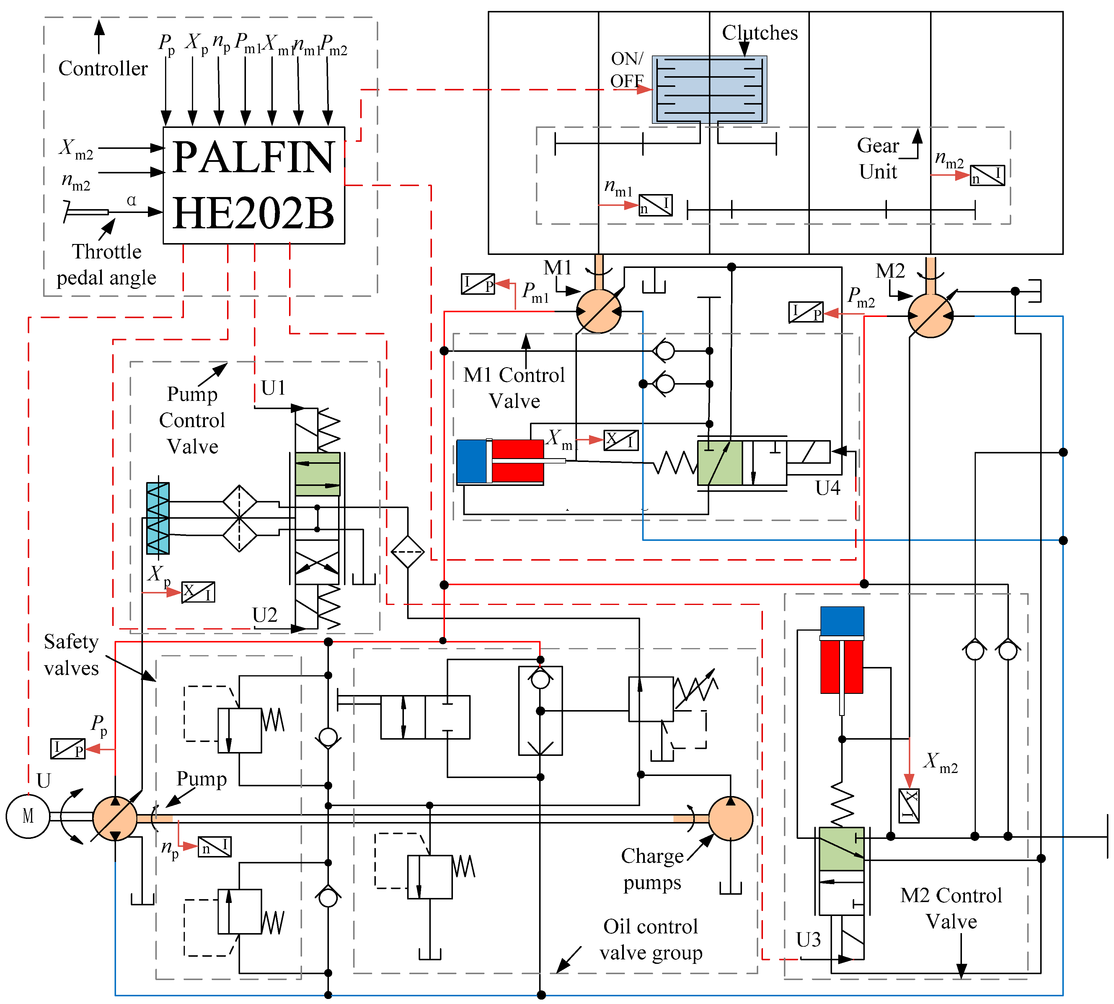
• A new variable-structure hydrostatic drive system is proposed to meet the driving requirements of wheel loaders, and its operating principles, structural layout, and basic control methods are analyzed.
• The mathematical model of the variable-structure hydrostatic drive is established, and the parameter relationships of the system’s main components are analyzed. The theoretical performance of the proposed drive system is analyzed through the establishment of a simulation model of the system.
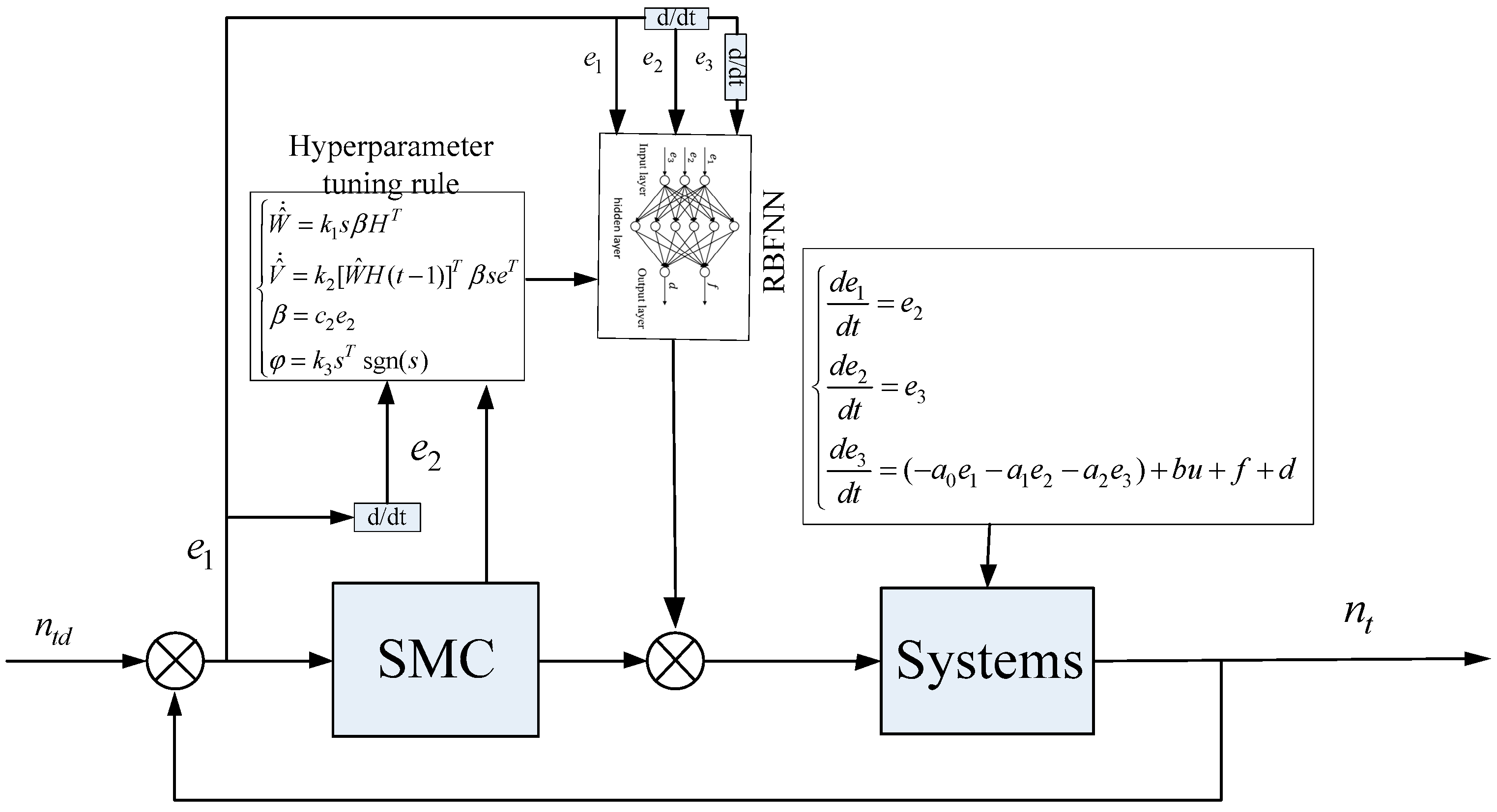
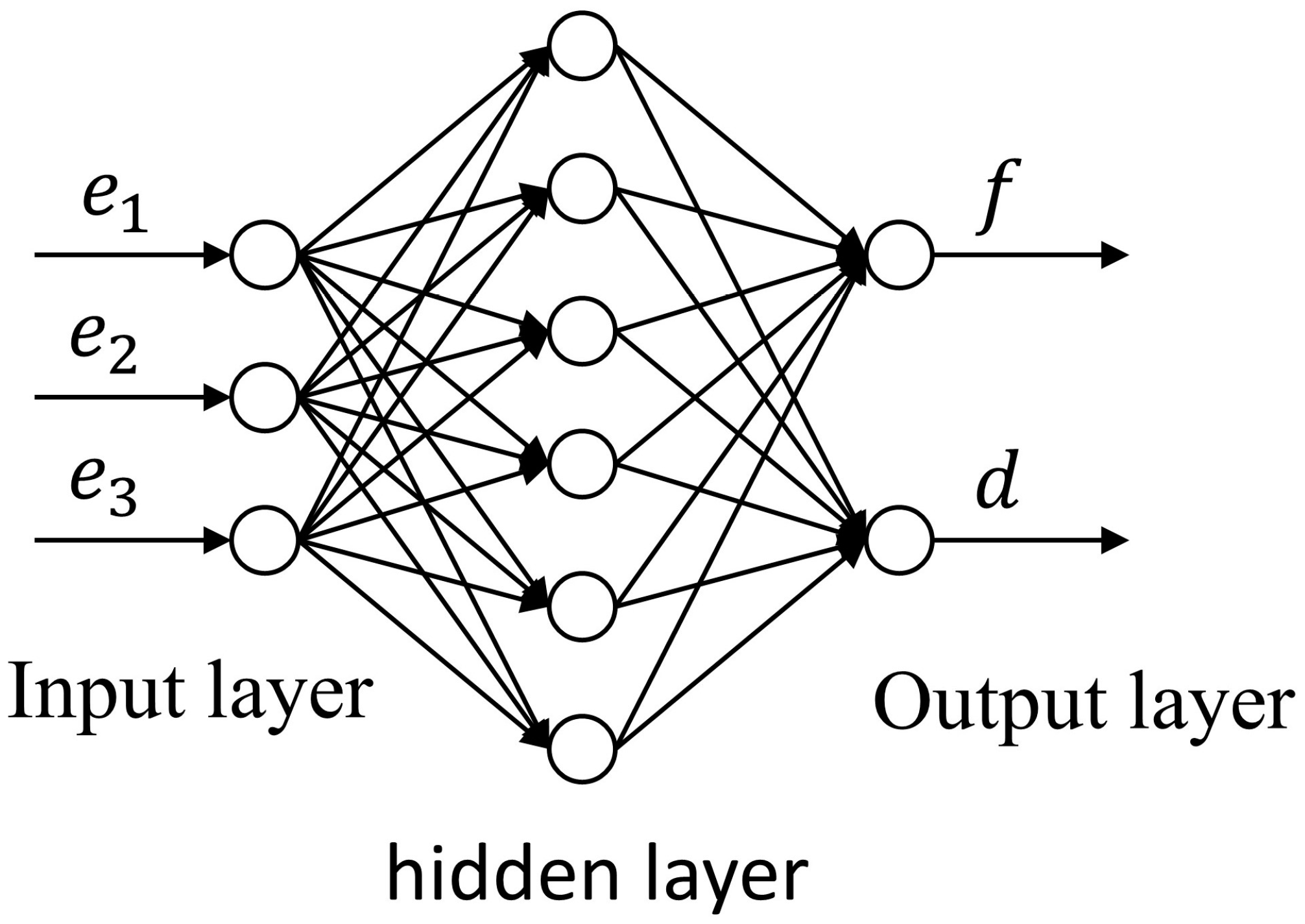
• An HST adaptive SMC strategy based on RBFNN optimization is proposed to address the displacement matching problem during the control process. The adaptive mechanism updates the RBFNN hyperparameters, improving the system’s tracking capability and robustness.
• The variable-structure hydrostatic drive system is successfully applied to actual loader products and put into commercial production.

This paper consists of five sections, with the following structure: Section 2 introduces the structural layout and operating principles of the variable-structure hydrostatic drive system, establishes the mathematical model of the system, and analyzes the parameter relationships of the system’s main components. Section 3 establishes the simulation model of the drive system, provides the design parameters of key components, verifies the theoretical performance of the system, proposes an HST adaptive sliding mode displacement matching control strategy based on RBFNN optimization, formulates hyperparameter adaptive update rules, and mathematically proves the stability and adaptability of the control strategy. Section 4 designs field tests for the loader equipped with the designed drive system and control strategy, verifying the actual working performance of the loader under V-shaped working conditions. Section 5 summarizes the entire paper and draws conclusions.

2. Working Principle and Mathematical Model

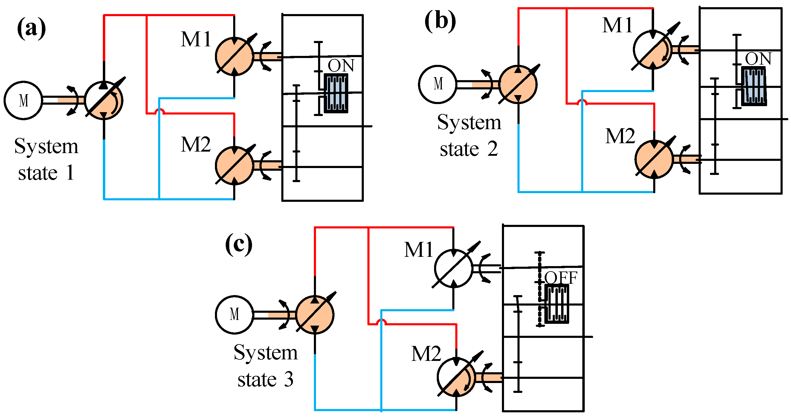
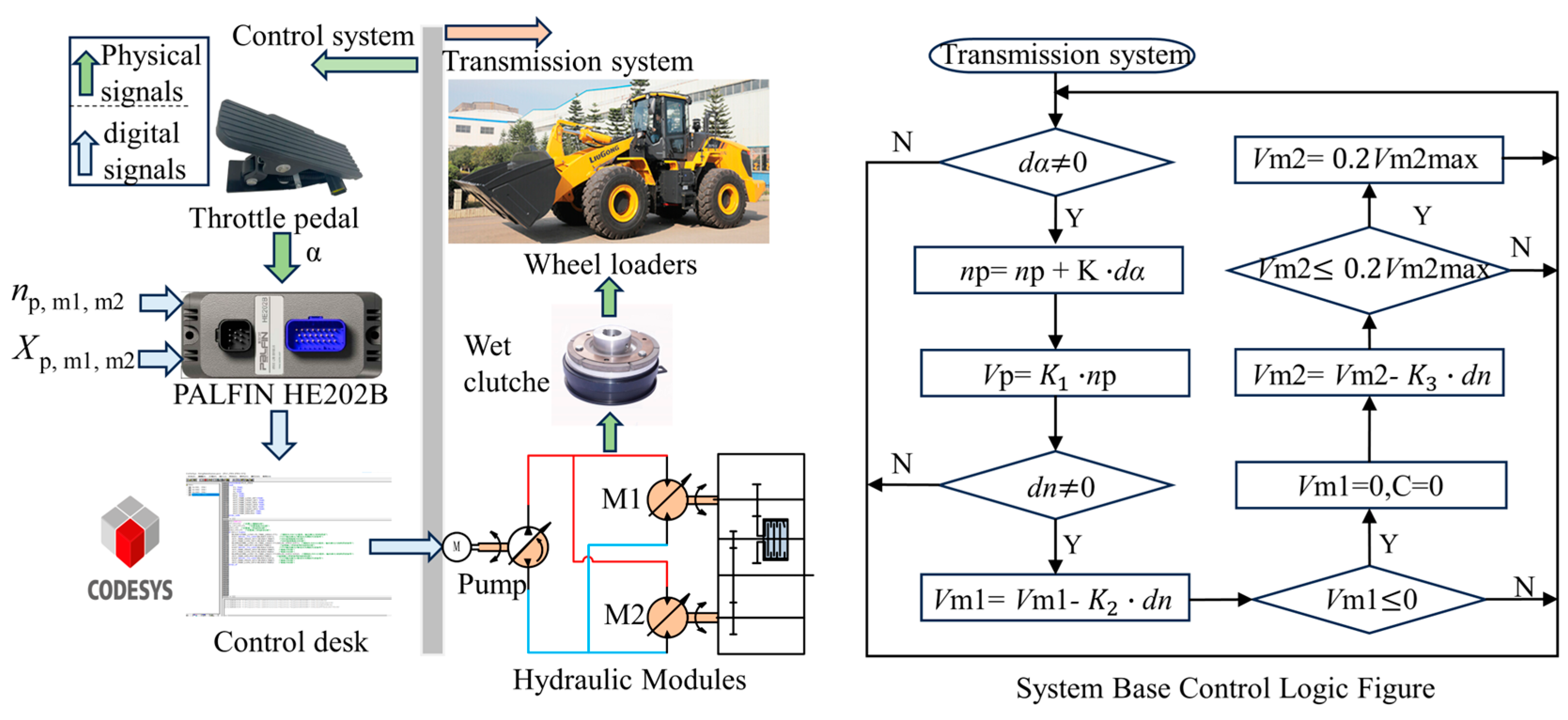
2.1. Variable Structure Hydrostatic Drive System

To improve the efficiency and maneuverability of the loader drive system, this paper proposes an adaptive variable-structure hydrostatic drive system, as shown in Figure 1. Unlike traditional mechanical drive systems using hydraulic torque converters, this system adopts a variable-structure hydrostatic drive system that combines hydraulic pumps with hydraulic motors. The power output from the engine is converted into hydraulic energy by the hydraulic pump, directly driving the hydraulic motor to rotate.

The engine is directly connected to the variable pump, and the power is input into the hydraulic circuit through the variable pump, achieving the transformation of mechanical energy into hydraulic energy. The high-displacement variable motor (M1) and the low-displacement variable motor (M2) convert hydraulic energy into kinetic energy under the driving force of the pressure difference between the inlet and outlet ports. The two motors are connected to the gearbox, and the power is combined in the gearbox through the gear set and then output to the drive shaft to propel the loader. The linkage between the M1 gear set and the output shaft is controlled by the clutch. When the displacement of M1 is small, the clutch can be disengaged to improve mechanical efficiency. The displacement of the pump and motors is controlled by the displacement control solenoid valve group, which is proportional to the input voltage. When the equivalent total displacement of the system changes, the pressure, flow rate, output speed, and torque of the system also change accordingly. By adjusting the prime mover engine speed, pump, and motor displacement, control of the system’s various parameters can be achieved. This drive system achieves an efficient automatic shifting drive, improving energy utilization efficiency.

The solid red line in Figure 1 represents the high-pressure oil circuit of the main oil pump during forward rotation. The red dashed line represents the control signal issued by the controller, and the red arrow represents the parameter signal detected by the sensor. The solid blue line represents the low-pressure oil circuit of the main oil pump during forward rotation. The gray dashed box represents the components enclosed, forming a functional unit. The green rectangular area represents the enabling side of the solenoid valve when the system is being driven in the forward direction. The blue rectangular area represents the low-pressure chamber of the hydraulic cylinder, and the red rectangular area represents the high-pressure chamber of the hydraulic cylinder.

2.2. Analysis of Control Principles for Variable Structure Hydrostatic Drive Systems

Figure 2 shows the control principle and simplified control strategy of a variable structure hydrostatic drive system. When the driver steps on the accelerator pedal, the change in pedal angle is collected by the vehicle controller. After calculation by the control program, the control signal is distributed to various controlled units in the drive system so that the engine speed increases in proportion to $K·d\alpha$ at the initial set speed. The displacement control voltage signal $U_1$ of the pump increases and $U_2$ decreases with the increase in speed, causing the pump displacement $V_{\mathrm{p}}$ to gradually increase. The system state is shown in Figure 3a. When the speed change value $dn$ of the loader wheel increases, the displacement $V_{\mathrm{m}1}$ of the hydraulic motor M1 will decrease proportionally until it decreases to zero. The system state is shown in Figure 3b. If $dn$ continues to increase, the wet clutch will disconnect, $C=0$, and the displacement $V_{\mathrm{m}2}$ of the hydraulic motor M2 will decrease proportionally until it reaches the set minimum displacement $V_{\mathrm{m}2\min }$. The system state is shown in Figure 3c. When $dn$ decreases, $V_{\mathrm{m}2}$ gradually increases to reach the set maximum displacement value $V_{\mathrm{m}2\max }$. When $dn$ further decreases, the clutch is engaged, $C=1$, and $V_{\mathrm{m}1}$ begins to increase to reach the set maximum displacement value $V_{\mathrm{m}1\max }$. When $dn$ remains unchanged, the system remains stable.

The driver can control the speed of the loader through the throttle pedal. The adaptive variable-structure hydrostatic drive system can automatically achieve seamless gear shifting according to the throttle requirements, realizing smooth adjustment of the loader’s speed. When rapid acceleration is needed, the driver only needs to press a button to directly switch the drive system to high-speed drive mode. When long-term, continuous transportation is required, speed maintenance can also be selected. The adaptive design can ensure stable tracking of target speeds. Pressing the brake or throttle pedal will automatically exit the speed maintenance setting, greatly reducing the fatigue caused by frequent gear-shifting operations for the loader driver and improving the efficiency of the loader.

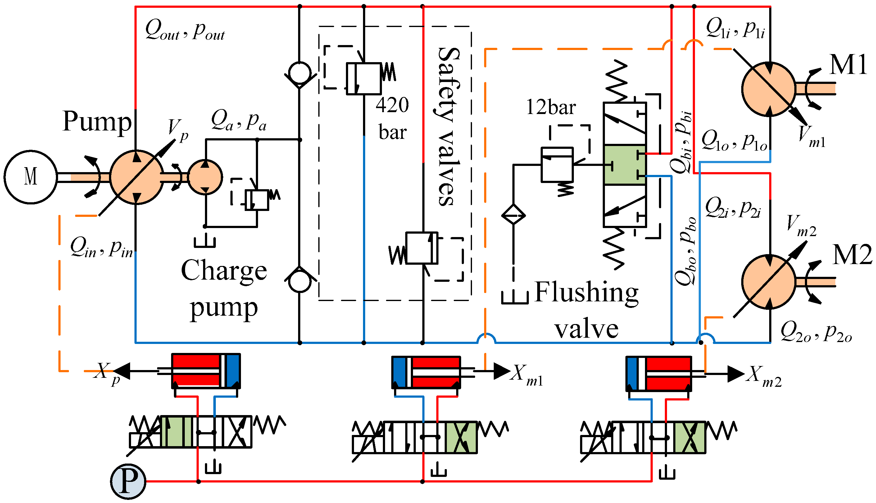
2.3. Analysis of the Variable Structure Hydrostatic Drive System and its Components

Analyzing fluid flow is crucial in variable-structure hydrostatic drive systems. The equivalent principle under the accelerated state in Figure 1 is shown in Figure 4.

$X_{\mathrm{p}}$, $X_{\mathrm{m}1},$ and $X_{\mathrm{m}2},$ respectively, represent the expansion and contraction displacement of the displacement control cylinder of the pump, motor M1, and motor M2. The flow rates at the inlet and outlet of the variable displacement pump are $Q_{\mathrm{in}}$ and $Q_{\mathrm{out}}$, respectively, and the pressures are $p_{\mathrm{in}}$ and $p_{\mathrm{out}}$, respectively. The flow rate of the charge pump is $Q_{\mathrm{a}}$, and the pressure is $p_{\mathrm{a}}$. The inlet and outlet oil flow rates of the flushing valve are $Q_{\mathrm{bi}}$ and $Q_{\mathrm{bo}}$, respectively, and the pressures are $p_{\mathrm{bi}}$ and $p_{\mathrm{bo}}$, respectively. The inlet flow rate of motor M1 is $Q_{1\mathrm{i}}$; the outlet flow rate is $Q_{1\mathrm{o}}$; the inlet pressure is $p_{1\mathrm{i}}$; and the outlet pressure is $p_{1\mathrm{o}}$. The inlet and outlet oil flow rates of motor M2 are $Q_{2\mathrm{i}}$ and $Q_{2\mathrm{o}}$, and the pressures are $p_{2\mathrm{i}}$ and $p_{2\mathrm{o}}$, respectively. Due to the interconnectivity between the various chambers in the hydraulic drive system, the pressure is related to the flow rate, and the following formula can be listed:

$$\left\{\begin{array}{l}{p}_{\mathrm{out}}=p_{1\mathrm{i}}=p_{2\mathrm{i}}\\ p_{\mathrm{in}}=p_{1\mathrm{o}}=p_{2\mathrm{o}}\\ Q_{\mathrm{out}}=Q_{\mathrm{in}}=n_{\mathrm{p}}{V}_{\mathrm{p}}-C_{\mathrm{tp}}(p_{\mathrm{out}}-p_{\mathrm{in}})\\ Q_{1\mathrm{o}}=Q_{1\mathrm{i}}=n_{\mathrm{m}1}{V}_{\mathrm{m}1}-C_{\mathrm{tm}1}(p_{1\mathrm{o}}-p_{1\mathrm{i}})\\ Q_{2\mathrm{o}}=Q_{2\mathrm{i}}=n_{\mathrm{m}2}{V}_{\mathrm{m}2}-C_{\mathrm{tm}2}(p_{2\mathrm{o}}-p_{2\mathrm{i}})\end{array}\right.,$$

(1)

where $n_{\mathrm{p}}$ and $C_{\mathrm{tp}}$ represent the pump speed and total leakage coefficient, respectively; $n_{\mathrm{m}1}$ and $C_{\mathrm{tm}1}$ represent the speed and total leakage coefficient of motor M1, respectively; and $n_{\mathrm{m}2}$ and $C_{\mathrm{tm}2}$ represent the speed and total leakage coefficient of motor M2, respectively.

2.3.1. Variable Displacement Control Valve Group

The displacement of the pump and motor is controlled by the variable displacement control valve group. The control principle is shown in Figure 4. One end of the oil inlet of the electromagnetic three-position four-way directional valve is connected to a stabilizing source, and the oil outlet is connected to a bidirectional hydraulic cylinder. By controlling the current on and off, the hydraulic oil flow direction is converted, driving the hydraulic cylinder to move back and forth and then driving the piston pump or motor to change the inclination angle of the swash plate, achieving control of the pump and motor displacement changes. The following formula can be listed:

$$V_{\mathrm{j}}=\frac{\pi }{4}{d}_{\mathrm{j}}^2{D}_{\mathrm{j}}{z}_{\mathrm{j}}\tan (\arcsin \frac{2X_{\mathrm{j}}}{D_{\mathrm{sj}}}),$$

(2)

where $d_{\mathrm{j}}$ represents the diameter of the plunger, $D_{\mathrm{j}}$ represents the diameter of the plunger distribution circle, $z_{\mathrm{j}}$ represents the number of plungers, $D_{\mathrm{sj}}$ represents the diameter of the swash plate, $X_{\mathrm{j}}$ represents the telescopic displacement of the displacement control cylinder, and $j=(p,m1,m2)$ represents the parameter subscripts of the pump, motor M1, and motor M2, respectively.

When the current I of the electromagnetic directional valve is positive, the right position is energized, and the hydraulic rod extends outward. When the current I is negative, the left position is energized, and the hydraulic rod retracts. The displacement of the hydraulic rod meets the following formula:

$${\dot{X}}_{\mathrm{j}}=\left\{\begin{array}{l}\frac{4C_{\mathrm{vj}}\Delta p_{\mathrm{j}}\sqrt{2\Delta p_{\mathrm{j}}}}{\pi d_{\mathrm{mj}}^2\sqrt{\rho }}I>0\\ -\frac{4C_{\mathrm{vj}}\Delta p_{\mathrm{j}}\sqrt{2\Delta p_{\mathrm{j}}}}{\pi {(d_{\mathrm{mj}}-d_{\mathrm{sj}})}^2\sqrt{\rho }}I\le 0\end{array}\right.,$$

(3)

where $C_{\mathrm{vj}}$ represents the pressure flow coefficient of the valve, i.e., the proportional coefficient of the linear segment of the pressure flow curve of steady-state laminar flow passing through the valve port under normal conditions; $∆p_{\mathrm{j}}$ represents the pressure difference at both ends of the valve port; $d_{\mathrm{mj}}$ and $d_{\mathrm{sj}}$ represent the piston diameter and piston rod diameter of the displacement control hydraulic cylinder, respectively; and $\rho$ represents the normal density of hydraulic oil.

2.3.2. Flushing Valve Group

In a closed circuit, the main circuit is composed of a pump and a motor. In addition to supplementing the oil with the charge pump, the external oil leakage from the pump and motor is also cooled and filtered through a bypass circuit. Due to the limited amount of cooling oil and insufficient replacement of the main circuit oil, there is a problem with the entire system temperature being too high. To improve this problem, a flushing valve (consisting of a low-pressure priority shuttle valve and an overflow valve) is installed in the main circuit, allowing the main circuit to force a small amount of overflow to the side circuit, improving cooling and filtration efficiency. As shown in Figure 1, the auxiliary function schematic diagram of the flushing valve is achieved by using a makeup oil circuit. Figure 4 shows the functional equivalence diagram of the flushing valve, and the formula can be listed as follows:

$$\left\{\begin{array}{l}{Q}_{\mathrm{bi}}=C_{\mathrm{q}}{A}_1\sqrt{\frac{2}{\rho }(p_{\mathrm{bi}}-12)}{p}_{\mathrm{bi}}\le p_{\mathrm{bo}}\\ Q_{\mathrm{bo}}=C_{\mathrm{q}}{A}_2\sqrt{\frac{2}{\rho }(p_{\mathrm{bo}}-12)}{p}_{\mathrm{bi}}\ge p_{\mathrm{bo}}\end{array}\right.,$$

(4)

where $C_{\mathrm{q}}$ represents the flow coefficient of the flushing valve; $A_1$ and $A_2$ represent the cross-sectional area of the oil ports on both sides of the flushing valve, respectively.

2.3.3. Dual Motor Coordination Relationship

When the system drives the vehicle to operate normally, both the flushing valve and safety valve remain normally closed, and the internal flow and pressure difference $∆p$ of the system are in dynamic equilibrium. The system flow balance equation at this time can be listed as:

$$n_{\mathrm{p}}{V}_{\mathrm{p}}-C_{\mathrm{tp}}\Delta p=n_{\mathrm{m}1}{V}_{\mathrm{m}1}+C_{\mathrm{tm}1}\Delta p+n_{\mathrm{m}2}{V}_{\mathrm{m}2}+C_{\mathrm{tm}2}\Delta p$$

(5)

In the system, the engine is connected to the variable displacement pump, and their speeds are always consistent. At any engine speed, the actual displacement of the variable displacement pump can be combined with the actual displacement of M1 and M2. In theory, each set of displacement combinations corresponds to a set of ideal output torque and ideal output speed, while the engine speed remains constant. According to the flow balance equation of the system, the expression for the ideal output speed can be derived:

$$n_{\mathrm{t}}=\frac{V_{\mathrm{p}}}{i_{\mathrm{m}0}(i_{\mathrm{m}1}{V}_{\mathrm{m}1}+i_{\mathrm{m}2}{V}_{\mathrm{m}2})}{n}_{\mathrm{p}},$$

(6)

where $i_{\mathrm{m}1}$ and $i_{\mathrm{m}2}$ are the gearbox reduction ratios of M1 and M2, respectively; $i_{\mathrm{m}0}$ is the drive axle reduction ratio; and $n_{\mathrm{t}}$ represents the output speed.

When the output power and output speed of the engine are determined, the output torque of the engine is also determined accordingly. Due to the direct rigid connection between the engine and pump, the input torque of the pump is determined and satisfies the relationship in Equation (7):

$$T_{\mathrm{p}}=\frac{V_{\mathrm{p}}\Delta p_{\mathrm{p}}{\eta }_{\mathrm{pt}}}{2\pi },$$

(7)

where $T_{\mathrm{p}}$ represents the input torque of the pump and ${\eta }_{\mathrm{pt}}$ represents the mechanical efficiency of the pump.

The output torques of M1 and M2, $T_{\mathrm{m}1}$ and $T_{\mathrm{m}2}$, are combined in the gearbox and output through the gearbox output shaft. They are finally transmitted to the drive shaft through the drive axle. The ideal output torque expression is Equation (8). Because the pressure difference of the hydraulic system remains constant within the system, the relationship between $T_{\mathrm{m}1}$, $T_{\mathrm{m}2}$ and the system pressure difference is similar to Equation (7). By combining Equation (8), the relationship between $T_{\mathrm{o}}$ and pressure difference can be obtained, as shown in Equation (9):

$$T_{\mathrm{o}}=i_{\mathrm{m}0}(T_{\mathrm{m}1}{i}_{\mathrm{m}1}{\eta }_{\mathrm{m}1\mathrm{t}}+T_{\mathrm{m}2}{i}_{\mathrm{m}2}{\eta }_{\mathrm{m}2\mathrm{t}}),$$

(8)

$$T_{\mathrm{o}}=\frac{i_{\mathrm{m}0}(i_{\mathrm{m}1}{V}_{\mathrm{m}1}+i_{\mathrm{m}2}{V}_{\mathrm{m}2})\Delta p{\eta }_{\mathrm{mt}}}{2\pi },$$

(9)

where $T_{\mathrm{o}}$ represents the ideal output torque; ${\eta }_{\mathrm{m}1\mathrm{t}}$ and ${\eta }_{\mathrm{m}2\mathrm{t}}$ represent the mechanical efficiency of M1 and M2, respectively; and ${\eta }_{\mathrm{mt}}$ represents the total mechanical efficiency.

In summary, the load torque balance equation for the dual variable motor is Equation (10), where $J_{\mathrm{t}}$ is the load moment of inertia, $B_{\mathrm{t}}$ is the damping coefficient, and $T_L$ is the load torque.

$$\Delta p{V}_{\mathrm{m}1}{i}_{\mathrm{m}1}+\Delta p{V}_{\mathrm{m}2}{i}_{\mathrm{m}2}=J_{\mathrm{t}}(\frac{d{n}_{\mathrm{m}1}}{dt}+\frac{d{n}_{\mathrm{m}2}}{dt})+B_{\mathrm{t}}(n_{\mathrm{m}1}+n_{\mathrm{m}2})+T_L$$

(10)

2.3.4. Charge Pump

In the oil control valve group in Figure 1, the charge pump has three main functions to provide oil replenishment for the closed system, namely the oil replenishment function. The other two auxiliary functions are to supply oil to the flushing valve and pump displacement control valve group, respectively. According to the analysis of the closed hydraulic system, the oil pump replenishes the system with cold oil, replacing the hot oil from the hydraulic pump and motor housing to achieve the cooling system function. After the system reaches a thermal equilibrium state, the system’s heating power is equal to the system’s heat dissipation power. Although the metal surface also emits heat, the small proportion is generally a negligible factor. Therefore, the cold oil added to the system per unit time reaches thermal equilibrium with the hot oil inside the system, satisfying Equation (11):

$$Q_{\mathrm{a}}=\frac{60(W_1+W_2+W_3+W_4)-(q_1+q_2+q_3+3q_c)p_{\mathrm{cx}}-(q_1+q_2+q_3)p_{\mathrm{a}}}{C\rho ({\theta }_1-{\theta }_2)-p_{\mathrm{cx}}-p_{\mathrm{a}}},$$

(11)

where $W_1$, $W_2$, $W_3$ and $W_4$, respectively, represent the heating powers of the pump, motor M1, motor M2, and pipeline; $q_1$, $q_2$, $q_3$, and $q_{\mathrm{c}}$, respectively, represent the leakage rates of the pump, motor M1, motor M2, and displacement control valve group; $p_{\mathrm{cx}}$ represents the set pressure of the flushing overflow valve; $C$ represents the specific heat capacity of hydraulic oil; and ${\theta }_1$ and ${\theta }_2$ represent the Celsius temperature of the hot oil source and the Celsius temperature of the cold oil source, respectively.

3. Simulation Methods and Control Strategies

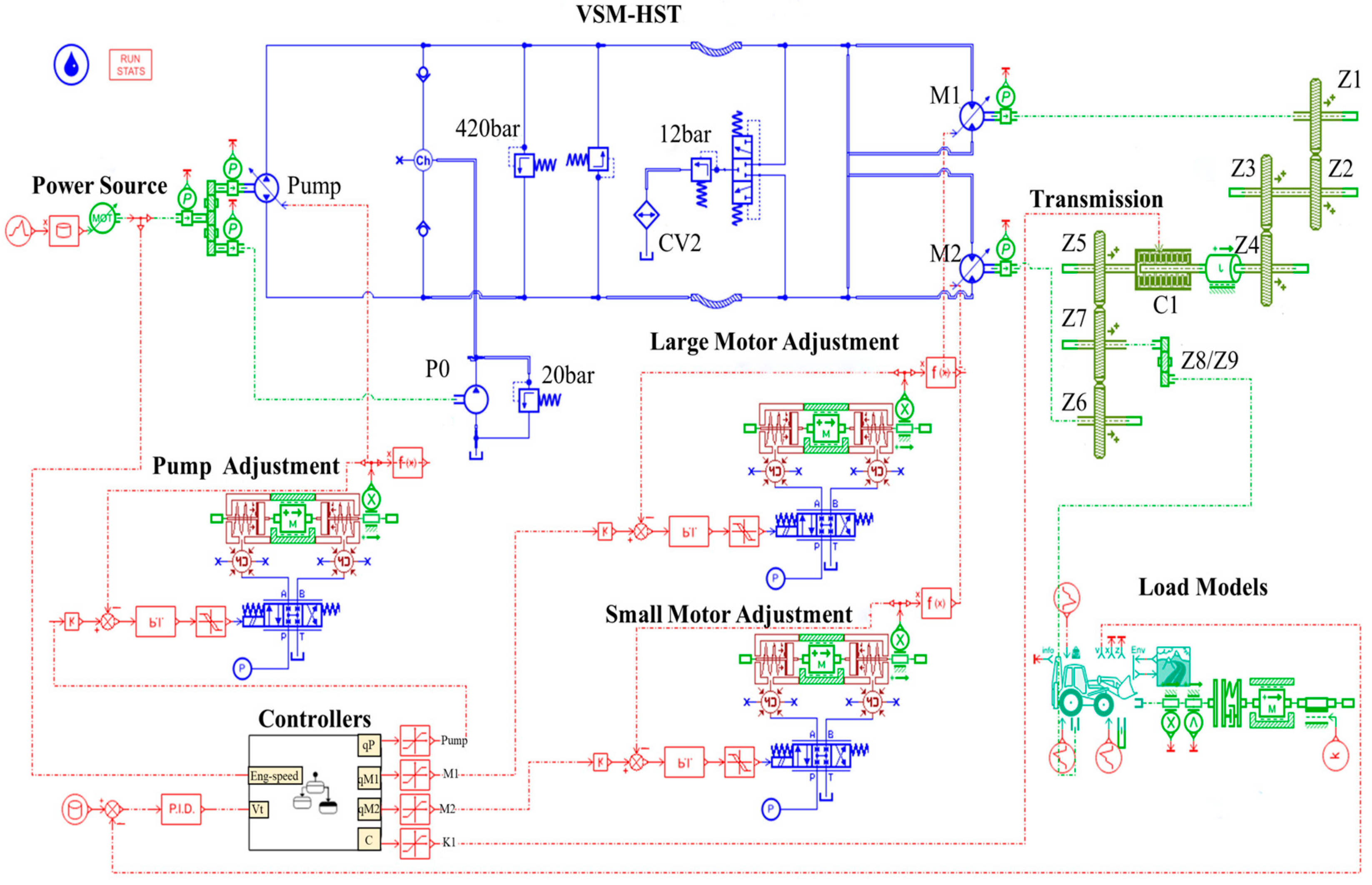
3.1. Simulation Method

Through simulation model validation experiments, research efficiency can be greatly improved [24]. Figure 5 shows the simulation model established based on the equivalent schematic diagram of the variable-structure hydrostatic drive system in Figure 4. The simulation model is built using AMESIM21.2 software, which is mainly divided into four parts: power source, variable structure hydrostatic drive system main body, gearbox, and load model. The main purpose is to verify the correctness of the principles of the designed driving system and control strategy. Therefore, except for setting key parameters known in the design, the model parameters are set by software default. The key parameters of the system are shown in

Table 1. Simulation model parameters.

Name	Value	Unit
Pump displacement	175.4	mL/r
Pump volumetric efficiency	96	%
Pump mechanical efficiency	94	%
Small motor displacement	164.2	mL/r
Small motor volumetric efficiency	92	%
Small motor mechanical efficiency	95	%
Large motor displacement	170.6	mL/r
Large motor volumetric efficiency	92	%
Large motor mechanical efficiency	92	%
Charge pump displacement	24.5	mL/r
Charge pump overflow pressure	2.5	MPa
Relief valve setting pressure	42	MPa
Flush valve setting pressure	2	MPa
Flush valve setting flow rate	20	L/min
Engine standard power	180	kW
Engine rated speed	2000	r/min
Maximum engine output torque	1187	Nm
Engine nominal fuel consumption	235	g/kW$·$h
Lowest engine fuel consumption at full load	230	g/kW$·$h
Drive axle transmission ratio (Z9/Z8)	24.67
Large motor transmission ratio [(Z2$·$Z4$·$Z7)/(Z1$·$Z3$·$Z5)]	3.23
Small motor transmission ratio (Z7/Z6)	1.44
Transmission mechanical efficiency	92	%

.

To ensure the accuracy of the simulation, the throttle opening and engine speed changes of a loader were measured using angle sensors and speed sensors, as shown in Figure 6. The data are imported into the simulation model control module in table form as input variables for simulation.

The external load on the loader varies during the operation process. To better fit the real working conditions, the load model used in this simulation is the loader’s whole vehicle model from the component library. The load parameter settings are shown in

Table 2. Load model parameters.

Name	Value	Unit
Overall vehicle mass	21,650	kg
Loading mass	7000	kg
Asphalt road resistance factor	0.010–0.018
Potholes road resistance factor	0.035–0.050
Gravel road resistance factor	0.020–0.025
Compression road resistance factor	0.050–0.150
Muddy road resistance factor	0.100–0.250
Iced road resistance factor	0.015–0.030
Dry sand road resistance factor	0.100–0.300
Wheel radius	0.75	m
Windward area	5	m2

. The shovel resistance and rolling resistance are shown in Figure 7. The changes in the overall vehicle weight and loading quality after the shovel loading operation are shown in Figure 8. The change in its value is an artificially set input to the simulation model based on previous experience in testing actual loaders in the V-type mode of operation.

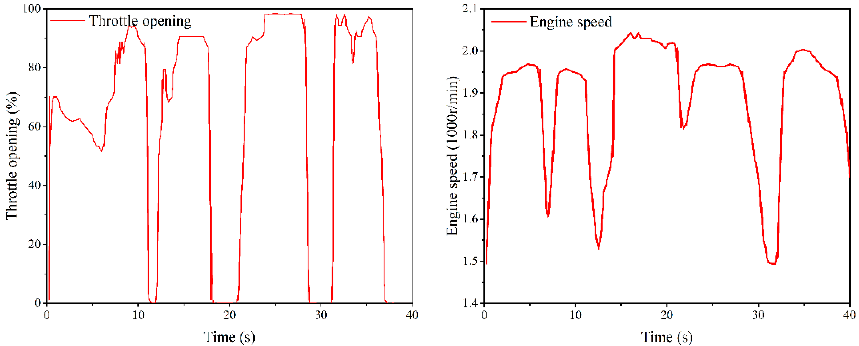
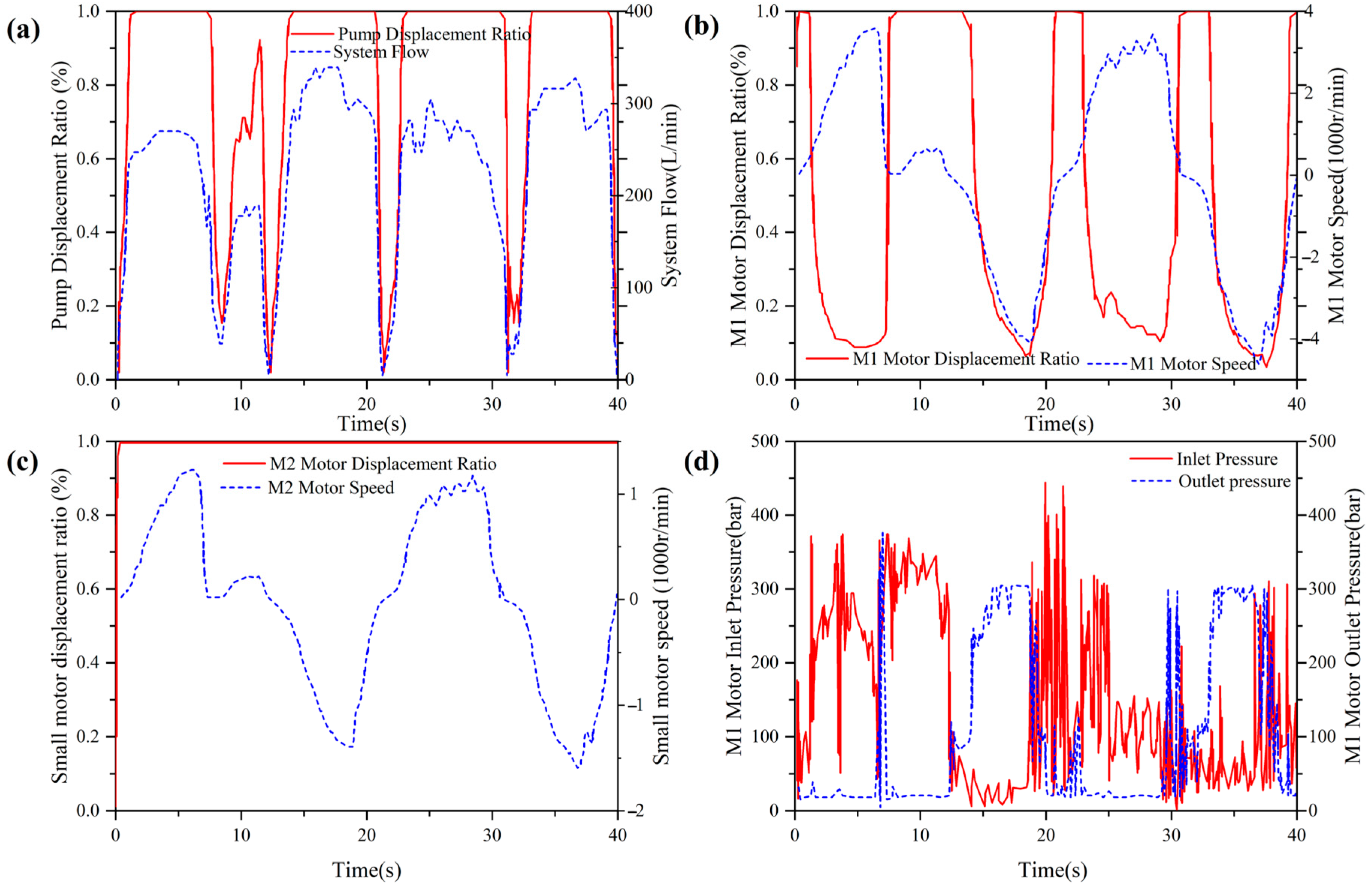
3.2. Simulation Model Validation

Figure 9 shows the simulation results of the simulation model based on the given input and control strategy in the set-load simulation environment. Figure 9a shows the pump displacement percentage and system flow value, which can be automatically adjusted smoothly according to the set strategy as the throttle opening changes. When the displacement of the pump changes, the oil supply of the transmission system also changes. The output speed of the large motor will change due to the combined effect of the fuel supply and its own displacement. Additionally, due to the coupling of the large and small motors, they act together on the power output shaft, so their output speed changes in the same proportion, as shown in Figure 9b,c. Due to the variation of the load model parameters, the driving torque of the bivariate motor hydrostatic system also changes. This leads to changes in the outlet pressure of the large and small motors. However, the pump and motors are controlled by the control strategy, and the system pressure and motor outlet pressure always fluctuate near the desired curve, as shown in Figure 9d. The simulation model can accurately reflect the characteristics and performance of the designed system because the simulation result curves match the expected results.

3.3. Displacement Matching Control Strategy

The control strategy of the designed drive system is to automatically generate control displacement values corresponding to the pump and motor based on throttle opening and engine speed as inputs, ultimately achieving control of vehicle speed. However, since the displacement control of the pump and motor is achieved through controlling the displacement control valve group, it is necessary to use the calculated control displacement value as input to develop a displacement matching control strategy to ensure the feasibility of the control strategy. From Equation (6), it can be seen that the system is a strongly coupled nonlinear control system with three inputs and one output. From Equation (7), it can be seen that the output torque is independent of the pump displacement and speed and is only controlled by the displacement changes of M1 and M2 and the size of the system pressure difference. When the input power and speed of the engine are determined, system control can be achieved by adjusting the displacement of the pump and motor.

3.3.1. The Design of the RBFNN Algorithm

The main goal of control is to achieve effective tracking of the actual output speed $n_{\mathrm{t}}$ against the target output speed $n_{\mathrm{td}}$, so the control effect can be represented by the actual deviation value $e$. When $e$ is equal to 0, it indicates that the control goal has been achieved. By controlling the input vector $u={[V_{\mathrm{p}},V_{\mathrm{m}1},V_{\mathrm{m}2}]}^T$, control of the system can be achieved, and the system control state equation [25] is Equation (12):

$$\left\{\begin{array}{l}\frac{d{e}_1}{dt}=e_2\\ \frac{d{e}_2}{dt}=e_3\\ \frac{d{e}_3}{dt}=(-a_0{e}_1-a_1{e}_2-a_2{e}_3)+bu+f+d\end{array}\right.,$$

(12)

where $e_1=e=n_{\mathrm{t}\mathrm{d}}-n_{\mathrm{t}}$ and $f$ represent external disturbance; $d$ represents changes in internal uncertain factors; and $F=f+d$ can be regarded as a whole and represents uncertain disturbance. $a_i\ge 0$ represents the coefficients of the state equation, obtained through training. This article adopts a three-layer RBFNN network structure, as shown in Figure 10. The input variables are tracking trajectory errors $e_1,e_2,{\mathrm{and}e}_3$, and the number of hidden layer neurons is six.

If the excitation output of the hidden unit $j$ is a basis function $H_j$, then the RBFNN approximation relationship can be written as Equation (13):

$$\left\{\begin{array}{l}F=WH(Ve)\\ H_j=\exp (-\frac{{‖V{e}_j-c_j‖}^2}{b_j^2})\end{array}\right.,$$

(13)

where $W$ represents the weight from the hidden layer to the output layer; $V$ represents the weight from the input layer to the hidden layer; and $c_j$ and $b_j$, respectively, represent the center position and width of the neuron.

Using the K-means clustering method [26], generate the initial center value of the basis function, update the input vector based on new input samples, and find the nearest center of the new input vector. The key data of the system are collected by sensors, and the new data set is pushed into the data stack of the dedicated register by the controller after processing, and the first-in-first-out principle is satisfied, so the data in the data stack is constantly updated, and the total data capacity of the data stack is 100 KB, and whenever the data in the data stack are all finished updating, all the data in the stack are automatically stored and taken as the new input samples, which are stored with the previous 9 times. samples to reconstruct a new data set and recalculate the clustering center value, which satisfies Equation (14):

$$j=\arg \min ‖Ve-c_j^n‖$$

(14)

where $c_j^n$ represents the center value of the jth basis function in the nth iteration, and the center point adjustment rule is carried out according to Equation (15):

$$c_j^n=\left\{\begin{array}{l}{c}_j^n+b_j(Ve-c_j^n)j=j(Ve)\\ c_j^{n}other\end{array}\right.$$

(15)

The width of the basis function is determined by the ratio of the farthest deviation distance $d_{j\max }$ from the center point to the number of hidden layers $h$ under the root sign, as shown in Equation (16):

$$b_j=\frac{d_{j\max }}{\sqrt{h}}$$

(16)

In order to simplify the design process, the weight value $V$ from the input layer to the hidden layer is set to 1. Only based on the error between the actual output result and the required result is the gradient descent principle used to update the weight between the hidden layer and the output layer. Given basis functions, there are optimal weights $\widehat{W}$ that achieve the smallest errors $\epsilon >0$, so that RBFNN approximates the best-fit function $\widehat{f}$ and satisfies the relationship in Equation (17):

$$\left\{\begin{array}{l}\max (f-\widehat{f})\le \epsilon \\ \widehat{W}=\arg \min [\sup (f-\widehat{f})]\end{array}\right.,$$

(17)

where $\delta =f-\widehat{f}$ represents the approximation error. Due to the presence of damping and resistance in actual systems, for the convenience of design, it is directly assumed that $\delta$ is bounded, so $‖W‖$ has the maximum value, and $\widehat{f}$ can continuously approach $f$.

3.3.2. SMC Algorithm Design

According to Equation (12), the sliding mode surface of the system is defined as Equation (18). In order to ensure that the system state reaches the sliding mode surface smoothly, it is also necessary to design a convergence rate to adapt to external disturbances, and the sliding mode convergence rate is given in Equation (19).

$$s=c_1{e}_1+c_2{e}_2+c_3{e}_3,$$

(18)

$$s=-\phi \mathrm{sgn}(s)-ks,$$

(19)

where $c_1{,c}_2{,c}_3,\mathrm{and}k$ are constants greater than zero, and their values can be determined by pole configuration, meeting the requirements of the Routh criterion. $\phi$ is the upper limit of the neural network error.

From Equations (12)–(19), the system control rate can be derived, as shown in Equation (20), where $n_{td}^{*}$ is the prior value of the actual output speed:

$$n_{td}^{*}=-{(b{c}_3)}^{-1}[c_1{e}_1+c_2{e}_2+c_{3}F-c_3{\stackrel{⃛}{n}}_{td}+ks+\phi \mathrm{sgn}(s)]$$

(20)

3.3.3. Stability Verification and Adaptive Adjustment

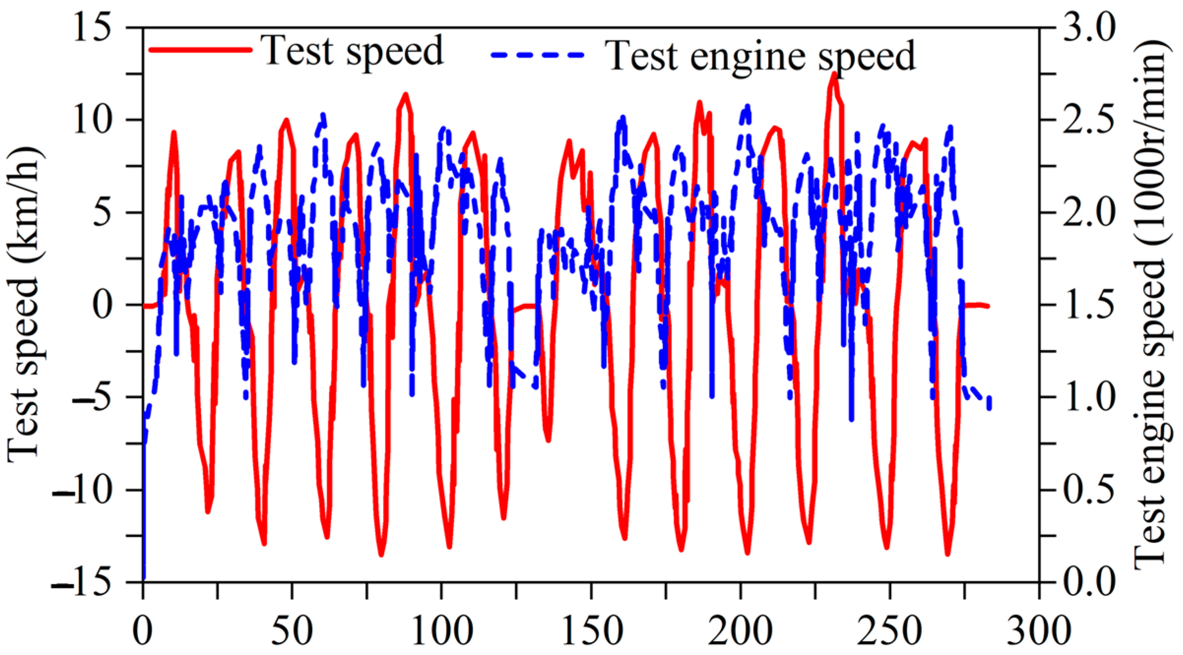
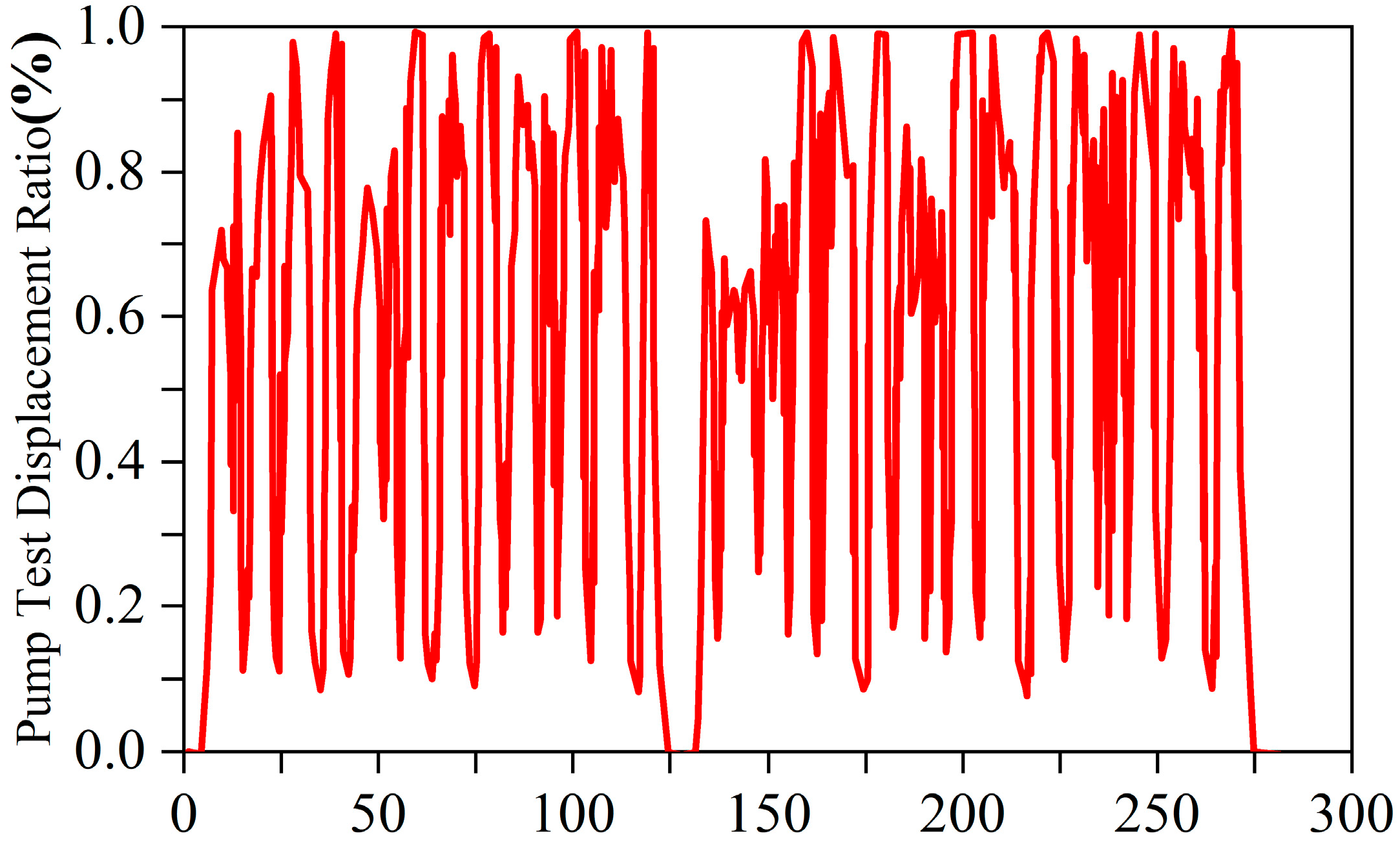
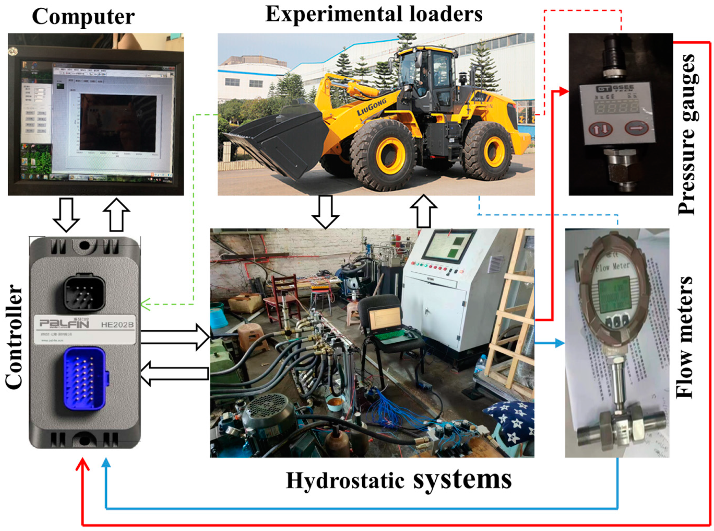
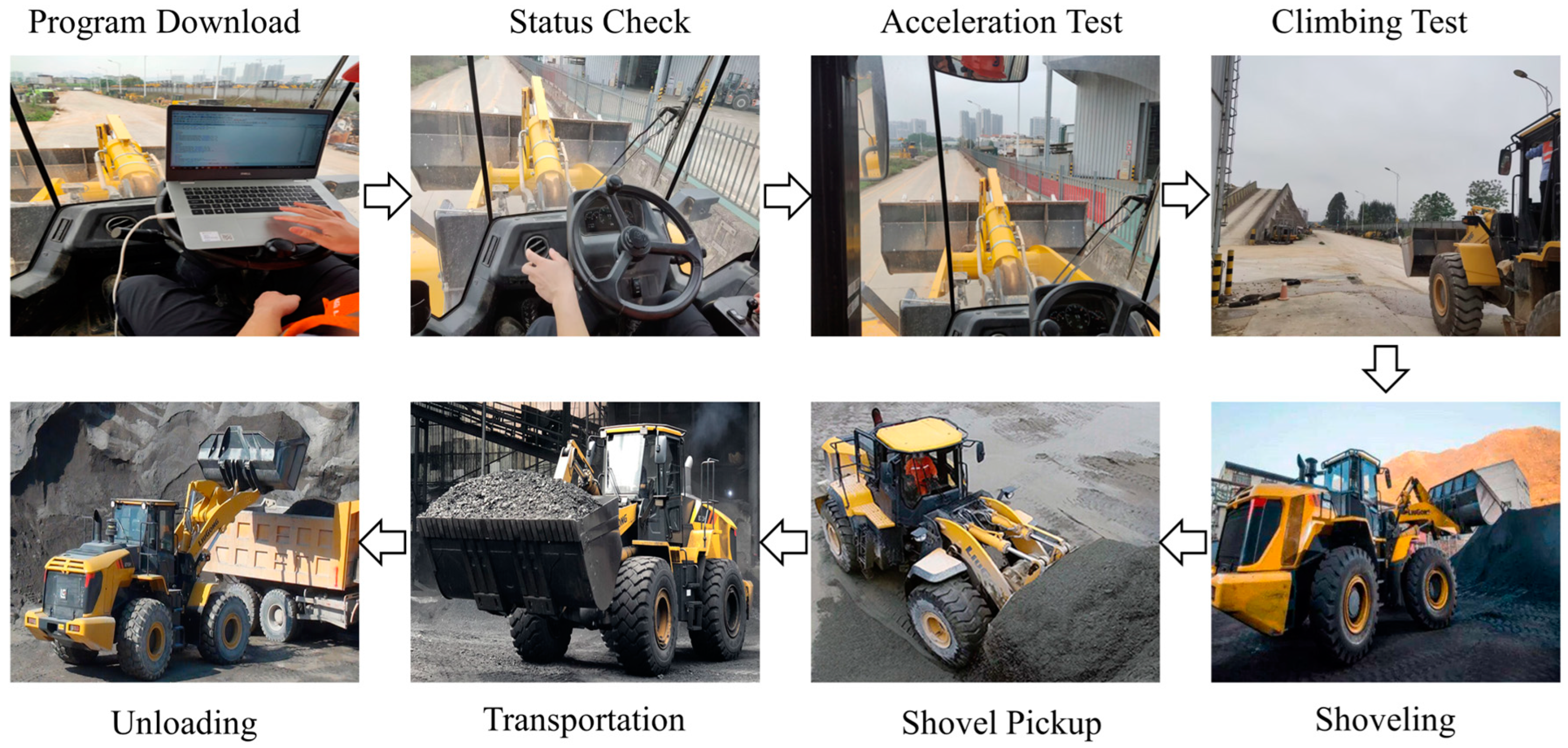
This article updates the hyperparameters of RBFNN through adaptive action, enabling system compensation to effectively cope with changes in uncertain factors. The algorithmic logic of the displacement matching control strategy is shown in Figure 11. The hyperparameter update rules are shown in Equation (21):

$$\left\{\begin{array}{l}\dot{\widehat{W}}=k_{1}s\beta H^T\\ \dot{\widehat{V}}=k_2{[\widehat{W}H(t-1)]}^T\beta s{e}^T\\ \beta =c_2{e}_2\\ \phi =k_3{s}^T\mathrm{sgn}(s)\end{array}\right.$$

(21)

where $k_1{,k}_2,\mathrm{and}{k}_3$ are constants greater than zero.

Based on the Lyapunov stability criterion [27,28,29,30], the system stability is proven, and the specific proof process is as follows:

$$V_1=\frac{1}{2}{s}^{T}s+\frac{1}{2k_1}{\tilde{W}}^T\tilde{W}+\frac{1}{2k_2}{\tilde{V}}^T\tilde{V}+\frac{1}{2k_3}{\tilde{\phi }}^2$$

(22)

where $\stackrel{\mathrm{~}}{W}=\widehat{W}-W$, and $\stackrel{\mathrm{~}}{V}$ represents the difference between the weights $\widehat{V}$ and $V$ of the best approximation input layer and the hidden layer, and $\stackrel{\mathrm{~}}{\phi }$ represents the error value of the neural network. We derived Equation (22) to obtain Equation (23), as shown below:

$${\dot{V}}_1=s^T\dot{s}+\frac{1}{k_1}{\tilde{W}}^T\dot{\tilde{W}}+\frac{1}{k_2}{\tilde{V}}^T\dot{\tilde{V}}+\frac{1}{k_3}\dot{\tilde{\phi }}\tilde{\phi }$$

(23)

Substituting Equations (20) and (21) into Equation (23) yields Equation (24):

$$\begin{array}{ll}{\dot{V}}_1& =s^T[c_1{e}_1+c_2{e}_2+c_3{e}_3]+\frac{1}{k_1}{\tilde{W}}^T\dot{\tilde{W}}+\frac{1}{k_2}{\tilde{V}}^T\dot{\tilde{V}}-\frac{1}{k_3}\dot{\tilde{\phi }}\tilde{\phi }\\ & =s^T[-ks-\phi \mathrm{sgn}(s)+\beta \tilde{F}]-\frac{1}{k_1}{\tilde{W}}^T\dot{\tilde{W}}-\frac{1}{k_2}{\tilde{V}}^T\dot{\tilde{V}}-\frac{1}{k_3}\dot{\tilde{\phi }}\tilde{\phi }\end{array}$$

(24)

where $\stackrel{\mathrm{~}}{F}$ represents the difference between the ideal output value $\widehat{F}$ and the actual output value $F$, i.e., $\tilde{F}=\widehat{F}-F=\tilde{W}H\left(\widehat{V}e\right)+\widehat{W}H\left(t-1\right)\left(\widehat{V}e\right)\tilde{V}e+w$. Replacing $\tilde{F}$ in Equation (24) yields Equation (25), as shown below:

$$\begin{array}{ll}{\dot{V}}_1=& s^T\beta \tilde{W}H(\widehat{V}e)+s^T\beta \widehat{W}H(t-1)(\widehat{V}e)\tilde{V}e+s^T\beta w-\\ & \frac{1}{k_1}{\tilde{W}}^T\dot{\widehat{W}}-\frac{1}{k_2}{\tilde{V}}^T\dot{\widehat{V}}-\frac{1}{k_3}\tilde{\phi }\dot{\tilde{\phi }}-s^{T}ks-s^T\tilde{\phi }\mathrm{sgn}(s)\\ & \le -s^{T}ks\le 0\end{array}$$

(25)

According to the Lyapunov stability principle, Equation (25) proves $V_1\dot{V_1}\le 0$, which indicates that the tracking error $e$ of the control system is asymptotically stable over a large range and can converge to zero. The errors of sliding surfaces, weights, and uncertain terms approximated by neural networks are bound.

4. Field Experiment

4.1. Test System

In order to verify the correctness and rationality of the control strategy formulated in the previous text and the simulation based on this strategy, this paper conducted a V-shaped cyclic loading operation using a test prototype. Before the start of the experiment, corresponding sensors, data collectors, etc., are installed at appropriate positions on the prototype to collect various parameter data during the experiment. The experimental equipment, as shown in Figure 12, uses a LiuGong862H hydrostatic loader for a V-shaped operation cycle test.

The experimental process is as follows: 1. The speed sensors are installed at the rear wheel drive shaft and the variable pump input shaft of the loader; the pressure sensor and flow sensor are installed in the hydraulic circuit; the formulated control strategy and algorithm are written into the vehicle controller; and then the sensors are connected to the controller separately; the controller is connected to the acquisition instrument through a bus. 2. The loader starts from the initial position in a forward direction, accelerates by stepping on the accelerator, maintains a constant speed by controlling the accelerator midway, releases the accelerator near the material pile, uses the resistance of the material pile to stop the loader, and then increases the accelerator to shovel and load. After the shovel loading is completed, it drives in reverse, accelerates first, then slows down to return to the initial position, and then starts driving forward towards the loading vehicle. Then it accelerates first and then slows down to reach the loading vehicle before unloading. After unloading, it reverses, accelerates first, and then decelerates to return to the initial position. During this homework process, sensors collect and record the engine speed, wheel speed, system pressure, system flow rate, pump, and motor displacement of the loader 3. The above process is repeated multiple times to collect the experimental data uniformly. The experimental process is shown in Figure 13.

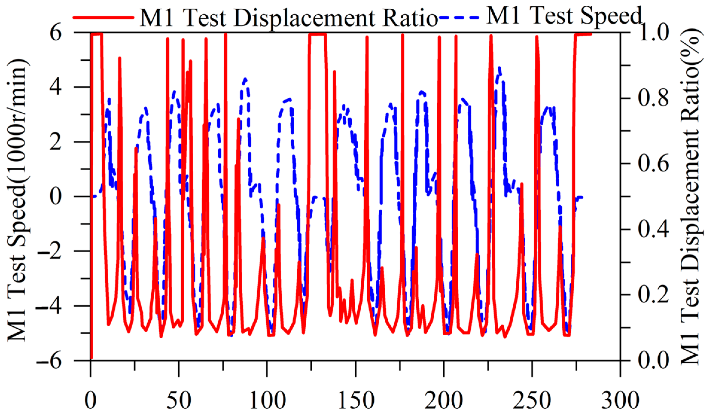
4.2. Experiment Results

The loader first completed three consecutive V-shaped operation conditions, idled for 15 s in the middle, and then conducted three V-shaped operations. The total test time was about 283 s, and the data sampling time was 0.5 s. The test data was exported from the vehicle controller after completing the entire test, and the entire process operated the loader frequently. It has been verified whether the drive system can ensure performance under high-frequency operation. The experimental data are as follows: Figure 14 shows the changes in the speed and engine speed of the loader; Figure 15 shows the changes in the speed and displacement ratio of the M1 motor test; Figure 16 shows the changes in the speed and displacement ratio of the M2 motor test; Figure 17 shows the changes in the inlet and outlet pressure of the variable pump test; and Figure 18 shows the changes in the displacement ratio of the pump test.

5. Conclusions

This study aims to improve the working efficiency of the loader transmission system and reduce fuel consumption. A new variable-structure hydrostatic drive system is proposed, and an HST adaptive SMC strategy based on RBFNN compensation is designed for the control problems of this system. Through theoretical analysis, simulation analysis, and experimental analysis, the structure, principles, and performance of the proposed new loader drive system are explained, leading to the following conclusions:

• Through simulation and field tests, it has been demonstrated that the proposed variable-structure hydrostatic drive system for loaders can meet the driving requirements of loaders in V-type working mode. The speed regulation process is smooth, and speed switching is seamless compared to traditional automatic speed regulation.
• The mathematical model established through principle analysis, structural analysis, and component analysis of the variable-structure hydrostatic drive system, along with simulation experiments, has proven to accurately predict and simulate the designed drive system.
• Addressing the displacement matching issue of the designed drive system, the proposed HST adaptive SMC strategy based on RBFNN compensation has been verified through experiments to effectively control and compensate the system. This ensures smooth speed fluctuation in situations such as climbing, rapid gear shifting, and sudden load changes, achieving automatic smooth gear shifting and improving the driving comfort and work efficiency of the operators.

References

1. Frank, B.; Kleinert, J.; Filla, R. Optimal control of wheel loader actuators in gravel applications. Autom. Constr. 2018, 91, 1–14. [Google Scholar] [CrossRef]
2. Wang, F.; Hong, J.; Ding, R.; Xu, B.; Fiebig, W.J. A Torque Conversion Solution to the Powertrain of Mobile Machine and Its Control Strategy. IEEE Trans. Veh. Technol. 2022, 71, 10361–10373. [Google Scholar] [CrossRef]
3. Oh, K.; Yun, S.; Ko, K.; Kim, P.; Seo, J.; Yi, K. An investigation of energy efficiency of a wheel loader with automated manual transmission. J. Mech. Sci. Technol. 2016, 30, 2933–2940. [Google Scholar] [CrossRef]
4. You, Y.; Sun, D.; Qin, D. Shift strategy of a new continuously variable transmission based wheel loader. Mech. Mach. Theory 2018, 130, 313–329. [Google Scholar] [CrossRef]
5. He, X.; Jiang, Y. Review of hybrid electric systems for construction machinery. Autom. Constr. 2018, 92, 286–296. [Google Scholar] [CrossRef]
6. Zhang, W.; Wang, J.; Du, S.; Ma, H.; Zhao, W.; Li, H. Energy Management Strategies for Hybrid Construction Machinery: Evolution, Classification, Comparison and Future Trends. Energies 2019, 12, 2024. [Google Scholar] [CrossRef]
7. Lin, T.; Wang, L.; Huang, W.; Ren, H.; Fu, S.; Chen, Q. Performance analysis of an automatic idle speed control system with a hydraulic accumulator for pure electric construction machinery. Autom. Constr. 2017, 84, 184–194. [Google Scholar] [CrossRef]
8. Wang, F.; Lin, Z.; Xu, B.; Fiebig, W. An Electric-Hydrostatic Energy Storage System for Hydraulic Hybrid Wheel Loader. IEEE Trans. Veh. Technol. 2022, 71, 7044–7056. [Google Scholar] [CrossRef]
9. Liu, F.; Wu, W.; Hu, J.; Yuan, S. Design of multi-range hydro-mechanical transmission using modular method. Mech. Syst. Signal Process. 2019, 126, 1–20. [Google Scholar] [CrossRef]
10. Wang, F.; Chen, J.; Xu, B.; Stelson, K.A. Improving the reliability and energy production of large wind turbine with a digital hydrostatic drivetrain. Appl. Energy 2019, 251, 113309. [Google Scholar] [CrossRef]
11. Han, X.; Su, W.; Zhao, H.; Zheng, Y.; Hu, Q.; Wang, C. Research of the hydrostatic transmission for deep-sea current energy converter. Energy Convers. Manag. 2020, 207, 112544. [Google Scholar] [CrossRef]
12. Comellas, M.; Pijuan, J.; Nogués, M.; Roca, J. Efficiency analysis of a multiple axle vehicle with hydrostatic transmission overcoming obstacles. Veh. Syst. Dyn. 2018, 56, 55–77. [Google Scholar] [CrossRef]
13. Rabbo, S.A.; Tutunji, T. Identification and analysis of hydrostatic transmission system. Int. J. Adv. Manuf. Technol. 2008, 37, 221–229. [Google Scholar] [CrossRef]
14. Zhou, S.; Walker, P.; Wu, J.; Zhang, N. Power on gear shift control strategy design for a parallel hydraulic hybrid vehicle. Mech. Syst. Signal Process. 2021, 159, 107798. [Google Scholar] [CrossRef]
15. Backas, J.; Ghabcheloo, R.; Huhtala, K. Gain scheduled state feedback velocity control of hydrostatic drive transmissions. Control. Eng. Pract. 2017, 58, 214–224. [Google Scholar] [CrossRef]
16. Fu, S.; Ren, H.; Lin, T.; Zhou, S.; Chen, Q.; Li, Z. SM-PI Control Strategy of Electric Motor-Pump for Pure Electric Construction Machinery. IEEE Access 2020, 8, 100241–100250. [Google Scholar] [CrossRef]
17. Wang, M.; Wang, Y.; Yang, R.; Fu, Y.; Zhu, D. A Sliding Mode Control Strategy for an ElectroHydrostatic Actuator with Damping Variable Sliding Surface. Actuators 2021, 10, 3. [Google Scholar] [CrossRef]
18. Kim, J.; Jin, M.; Choi, W.; Lee, J. Discrete time delay control for hydraulic excavator motion control with terminal sliding mode control. Mechatronics 2019, 60, 15–25. [Google Scholar] [CrossRef]
19. Li, H.; Chen, B.; Ma, B.; Zhang, H. Fuzzy adaptive PID synchronization control of hydrostatic transmission for high-speed overlay vehicles. J. Agric. Mach. 2010, 41, 16–19. [Google Scholar]
20. Huo, D.; Chen, J.; Zhang, H.; Shi, Y.; Wang, T. Intelligent prediction for digging load of hydraulic excavators based on RBF neural network. Measurement 2023, 206, 112210. [Google Scholar] [CrossRef]
21. Deng, P.; Zeng, L.; Liu, Y. RBF Neural Network Backstepping Sliding Mode Adaptive Control for Dynamic Pressure Cylinder Electrohydraulic Servo Pressure System. Complexity 2018, 2018, 4159639. [Google Scholar] [CrossRef]
22. Li, X.; Gao, H.; Xiong, L.; Zhang, H.; Li, B. A Novel Adaptive Sliding Mode Control of Robot Manipulator Based on RBF Neural Network and Exponential Convergence Observer. Neural Process. Lett. 2023, 55, 10037–10052. [Google Scholar] [CrossRef]
23. Fu, Y.; Zhou, X.; Wan, B.; Yang, X. Decoupled adaptive terminal sliding mode control strategy for a 6-DOF electro-hydraulic suspension test rig with RBF coupling force compensator. Proc. Inst. Mech. Eng. Part C J. Mech. Eng. Sci. 2023, 237, 4339–4357. [Google Scholar] [CrossRef]
24. Ma, W.; Xie, D.; Wang, Z.; Ran, Z.; Liu, C.; Wang, S. Modeling, calculation, and analysis of torsional vibration characteristics of the hydrodynamic transmission system in engineering vehicle. Proc. Inst. Mech. Eng. Part D J. Automob. Eng. 2022, 236, 1824–1839. [Google Scholar] [CrossRef]
25. Feng, H.; Song, Q.; Ma, S.; Ma, W.; Yin, C.; Cao, D.; Yu, H. A new adaptive sliding mode controller based on the RBF neural network for an electro-hydraulic servo system. ISA Trans. 2022, 129, 472–484. [Google Scholar] [CrossRef] [PubMed]
26. Yu, H.; Wen, G.; Gan, J.; Zheng, W.; Lei, C. Self-paced Learning for K-means Clustering Algorithm. Pattern Recognit. Lett. 2020, 132, 69–75. [Google Scholar] [CrossRef]
27. Cerman, O.; Hušek, P. Adaptive fuzzy sliding mode control for electro-hydraulic servo mechanism. Expert Syst. Appl. 2012, 39, 10269–10277. [Google Scholar] [CrossRef]
28. Chiang, M.-H.; Lee, L.-W.; Liu, H.-H. Adaptive fuzzy controller with self-tuning fuzzy sliding-mode compensation for position control of an electro-hydraulic displacement-controlled system. J. Intell. Fuzzy Syst. 2014, 26, 815–830. [Google Scholar] [CrossRef]
29. Zhang, J.; Chen, D.; Shen, G.; Sun, Z.; Xia, Y. Corrigendum to “Disturbance observer based adaptive fuzzy sliding mode control: A dynamic sliding mode surface approach” [Automatic 129 (2021) 109606]. Automatic 2022, 142, 110413. [Google Scholar] [CrossRef]
30. Singh, V. A note on Routh’s criterion and Lyapunov’s direct method of stability. Proc. IEEE 1973, 61, 503. [Google Scholar] [CrossRef]
Figure 1. Variable structure hydrostatic drive system.
Machines 12 00238 g001
Figure 2. Control principle of the variable structure hydrostatic drive system.
Machines 12 00238 g002
Figure 3. Changes in system operation status: (a) system startup or ultra-low speed driving state; (b) system low-speed state; and (c) system high-speed state.
Machines 12 00238 g003
Figure 4. Equivalent schematic diagram of the driving system under acceleration, the red color indicates high pressure oil, the blue color indicates low pressure oil, the black solid line indicates the auxiliary oil circuit, and the green color indicates that the solenoid valve is energized when driven in the positive direction.
Machines 12 00238 g004
Figure 5. Simulation model of the variable-structure hydrostatic drive system.
Machines 12 00238 g005
Figure 6. Throttle opening and engine speed.
Machines 12 00238 g006
Figure 7. Changes in shovel load resistance and rolling resistance. The graph shows two lines: the solid red line represents shoveling resistance, which is the resistance of the material to bucket insertion when the loader bucket is inserted into the stockpile, and the dashed blue line represents rolling resistance, which is the resistance that the loader wheels need to overcome to keep rolling.
Machines 12 00238 g007
Figure 8. Changes in material mass and loader mass. The red line represents the mass of the material in the bucket, while the blue line represents the total mass of the loader.
Machines 12 00238 g008
Figure 9. Simulation results: (a) pump displacement percentage and system flow rate; (b) displacement percentage and output speed of motor M1; (c) percentage and output speed of motor M2; and (d) pressure fluctuations at the inlet and outlet ports of motor M1.
Machines 12 00238 g009
Figure 10. RBFNN network structure.
Machines 12 00238 g010
Figure 11. Algorithm control logic diagram.
Machines 12 00238 g011
Figure 12. Experimental testing equipment, the red solid line indicates the pressure signal, the red dashed line indicates the electrical signal of the pressure indicator, the blue solid line indicates the flow signal, the blue dashed line indicates the electrical signal of the flow indicator, the green dashed line indicates the electrical signal of the loader status information, and the white arrow indicates the direction of the information transmission process.
Machines 12 00238 g012
Figure 13. Experimental process.
Machines 12 00238 g013
Figure 14. Changes in loader test speed and engine speed. The engine changes continuously with the speed of the vehicle, and there is no sudden change in engine speed, resulting in a stuck or stalled state. This indicates that the drive system can effectively adjust the matching problem between load and speed.
Machines 12 00238 g014
Figure 15. Changes in motor M1 test speed and displacement ratio. The speed change of M1 is synchronized with the speed change. The displacement can be quickly adjusted according to the speed demand.
Machines 12 00238 g015
Figure 16. Changes in motor M2 test speed and displacement ratio. M2 does not participate in adjustment at low speeds, the displacement remains stable, and the speed changes with the vehicle speed.
Machines 12 00238 g016
Figure 17. Pressure changes at the inlet and outlet of the variable pump test. The system pressure fluctuates continuously in a controllable range with changes in vehicle speed, and there is no abnormal decrease or increase in pressure. This indicates that the driving system can effectively adjust the engine input power according to load changes during the entire test process to ensure stable vehicle speed.
Machines 12 00238 g017
Figure 18. Changes in the pump test displacement ratio.
Machines 12 00238 g018