Adaptive Terminal Sliding Mode Trajectory Tracking Control for Autonomous Vehicles Considering Completely Unknown Parameters and Unknown Perturbation Conditions

Abstract

In the actual implementation of autonomous vehicle controller and related applications, it is difficult to obtain all the actual parameters of the vehicle. Considering factors such as uneven pavement and different pavement conditions, it is difficult to accurately establish the vehicle dynamic system model. Based on the non-singular terminal sliding mode and adaptive control theory, this paper establishes a trajectory tracking control strategy for an autonomous vehicle with unknown parameters and unknown disturbances. Firstly, the complex trajectory tracking problem is decoupled from the position and heading angle tracking problem, and the preview error equation is established. Secondly, a non-singular terminal sliding mode (NTSM) controller is established to stabilize the trajectory tracking error to the origin in a finite time, and adaptive laws are proposed to estimate the unknown vehicle parameters to adapt to environmental changes. Through the CarSim–Matlab platform, typical working conditions are implemented to verify the proposed controller. Our experimental outcomes affirm that the NTSM controller effectively guarantees the autonomous vehicle’s accurate following of the reference path, ensuring smooth control inputs throughout the entire process.

1. Introduction

With the development of driverless technology and the automobile manufacturing industry, Automated Ground Vehicles (AGVs) have gradually become a hot topic in society. AGVs refer to the intelligent collaboration of vehicle, road, human, cloud, and other information to realize the development of human beings towards the development of smart cities. At the same time, the mature intelligent network technology also has the advantages of reducing traffic accidents, alleviating traffic pressure, reducing the work intensity of drivers, etc. and realizing safety, intelligence, comfort, and energy saving in the process of automobile driving. Therefore, AGVs have a broad application prospect in the Intelligent Transportation System [1,2,3,4,5,6]. And as an important part of intelligent connected vehicle technology, trajectory tracking technology involves how to steer the vehicle to make the vehicle travel along the reference path under the premise of ensuring the safety and comfort of the driver. Since vehicles need to travel in various complex and changing environments, most research is focused on how to design robust control algorithms [7,8,9,10,11,12].

The objective of trajectory tracking control for autonomous vehicles is to converge the distance error and direction error between the actual path and the reference path to zero during driving and to implement the accurate tracking of the reference path. Currently, trajectory tracking controllers are mainly developed using kinematic and dynamic vehicle models. The kinematic model studies the vehicle motion, describing the magnitude and direction relationships between the vehicle’s spatial position, velocity, and acceleration. A trajectory tracking controller based on the kinematic model is proposed [13]. However, the kinematic model controllers can only work in limited driving environments due to ignoring the vehicle dynamics. The dynamic model considers the vehicle mass and introduces force and energy, so it not only studies the vehicle motion but also the force analysis in the vehicle motion. Therefore, vehicle dynamics models are more applicable to the mainstream trajectory tracking control methods [14,15,16,17,18,19].

In the field of trajectory tracking control, commonly used control methods include classical PID control [20], linear–quadratic regulator (LQR) methods [21], back stepping, adaptive control, robust control, the model predictive control (MPC) method, etc. PID and LQR control are effective and mature algorithms, but they are generally difficult to be applied to complex working conditions; both cannot exhibit high robustness [22,23] because the classical PID controller operates on the principle of “using error feedback to eliminate errors”. However, since the system output exhibits some inertia, it cannot undergo sudden changes. On the other hand, the target value can change abruptly. Therefore, it is unreasonable to make a quantity that cannot change abruptly track a quantity that can. Hence, PID controllers are not well suited for complex environments. Additionally, the relationship between system input and output may not always be accurately described by linear relationships, so the LQR method also has limitations for complex systems. The MPC method has been widely used to predict future states of the vehicle dynamics model in a finite time to predict the future state of the vehicle dynamics model and minimize the path tracking error within the prediction range under the constraints, e.g., an optimal trajectory optimization strategy for AGVs to cooperatively carry out mainline platooning and on-ramp merging [24]. A hierarchical control method based on the MPC approach for AGVs to achieve efficient and safe parallel operation is proposed [25]. MPC is used to achieve the trajectory tracking of intelligent vehicles while ensuring the stability and safety of intelligent vehicle driving [26]. However, it requires a large amount of computation in calculating the optimal solution and has high requirements for computer hardware.

Sliding mode controllers can exhibit high robustness to uncertainties in complex vehicle systems while tracking a reference path. Algorithms based on the sliding mode control theory can reach the sliding mode surface in finite time, and once the system reaches the sliding mode surface, it can de-compensate for the perturbations. In the sliding mode control method, the introduction of a sign function to compensate for disturbances can cause the system to need to traverse back and forth and slide on the sliding mode surface as it converges to the sliding mode surface. So, the first-order linear sliding mode controller exhibits a large chattering phenomenon due to high-frequency control switching. Therefore, researchers have made improvements and [27] propose a second-order quasi-continuous (QC)-based trajectory tracking strategy to track the desired transition path for generating the front wheel turn angle of the self-driving vehicle so that the distance and direction errors between the vehicle and the reference path converge to zero. A robust AGV trajectory tracking control strategy based on the non-singular terminal sliding mode (NTSM) and active disturbance rejection control (ADRC) is proposed to estimate and compensate the unmodeled dynamics and unknown external perturbations of the system in real time using an extended state observer [28]. The NTSM can effectively suppress a large chattering phenomenon and ensure that the tracking error converges to zero in a finite time even in the presence of disturbances. Furthermore, a continuous non-singular fast terminal sliding mode control method, which effectively ensures the continuity of the sliding mode surface and the non-singularity of the system and improves the convergence speed and control accuracy of the system when approaching the sliding mode surface, is proposed in [29,30]. The NTSM method is also used to complete pose control [31]. The NTSM is different from the traditional SMC in that the introduction of the exponential law makes the convergence faster to cope with external disturbances, while the adaptive laws can be used to eliminate parameter uncertainties and minimize the boundary layer of the sliding mode surface [32].

Based on the above discussion, an adaptive terminal sliding mode trajectory tracking control strategy is proposed for autonomous vehicles. The contributions of this paper are outlined as follows:

(1)

A non-singular terminal sliding model control protocol is proposed to track the ideal trajectory and guarantee the preview error converging to zero in a finite time. The chattering issue encountered by the conventional sliding mode controller is effectively addressed by the proposed method.

(2)

The proposed controller is integrated with the adaptive algorithm, eliminating the need for prior knowledge of vehicle parameters and perturbation bounds. This ensures a more flexible and robust system capable of dynamically adjusting to varying conditions.

(3)

To illustrate the effectiveness of the proposed method, the CarSim–Matlab joint simulations and real-world experimental studies are conducted. The proposed method is compared with the conventional controllers and verified under various driving conditions.

2. Modeling and Problem Description

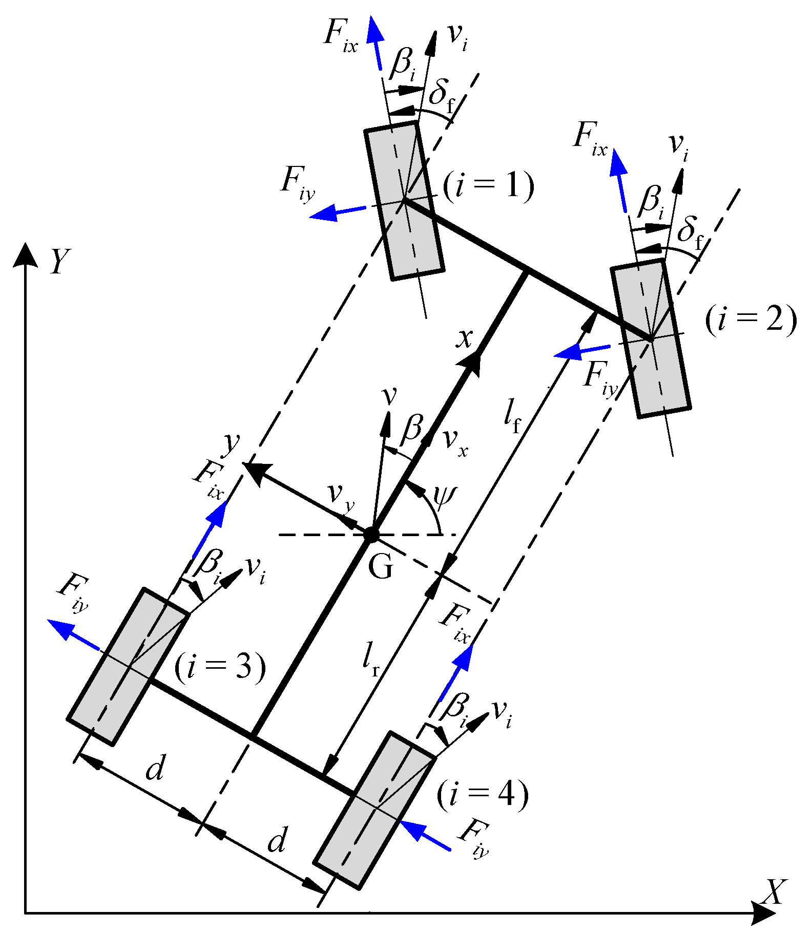
2.1. Modeling of Vehicle Three-Degrees-of-Freedom Dynamics

The three-degrees-of-freedom four-wheel dynamics model and coordinate system are shown in Figure 1. The vehicle dynamics model is modeled as follows [33,34].

The longitudinal equation of motion along the x-axis is as follows:

$$m({\dot{v}}_x-v_y\gamma )=F_{fax}\cos {\delta }_f+F_{rax}-F_{fay}\sin {\delta }_f$$

(1)

where F_fax = F_1x + F_2x, F_rax = F_3x + F_4x, and F_fay = F_1y + F_2y.

The equation of lateral motion along the y-axis is as follows:

$$m({\dot{v}}_y+v_x\gamma )=F_{fax}\sin {\delta }_f+F_{fay}\cos {\delta }_f+F_{ray}$$

(2)

where F_ray = F_3y + F_4y.

The yaw motion of the z-axis is as follows:

$$I_z\dot{\gamma }=F_{fax}{l}_f\sin {\delta }_f-d{F}_{fby}\sin {\delta }_f+F_{fay}{l}_f\cos {\delta }_f-l_f{F}_{ray}$$

(3)

where F_fby = F_2y − F_4y.

Figure 1 shows the vehicle dynamics model used in this paper, and its main parameters are shown in

Table 1. Vehicle model variables.

Symbolic	Unit	Description
m	kg	Vehicle mass
lf	m	Distance from center of gravity (CG) to front axle
lr	m	Distance from CG to rear axle
δf	rad	Steering angle of front wheels
d	m	Distance from CG to left/right wheel
i		Wheel ID, and i = 1, 2, 3, 4
Iz	kg·m2	Yaw moment of inertia of vehicle
γ	rad/s	Yaw rate of vehicle
β	rad	Sideslip angle of vehicle
βi	rad	Sideslip angle of wheel i
v	m/s	Total velocity of CG
vi	m/s	Speed of wheel i

.

When the vehicle is in motion, considering the energy loss caused by the sideslip of the tires, the longitudinal driving force on the tires can be obtained as

$$F_{ix}=(T_i-\Delta T_i)/R$$

(4)

Where T_i is the input torque of wheel I, and ΔT_i is the torque loss. R is the wheel radius.

The lateral force of a tire is related to the cornering stiffness and the sideslip angle, and the value of the cornering stiffness is determined by the road conditions and the normal force on the tire. Defining the actual cornering stiffness of wheel i as a variable, which can be varied with the tire conditions, the lateral force of wheel i can be written as follows:

$$F_{iv}=c_i{\beta }_i$$

(5)

where c_i is the cornering stiffness of wheel i, and β_i is the sideslip angle of wheel i.

The actual cornering stiffness of each wheel can be expressed as follows:

$$\left\{\begin{array}{l}{c}_1=c_f/2+\Delta c_1,c_2=c_f/2+\Delta c_2\\ c_3=c_f/2+\Delta c_3,c_4=c_f/2+\Delta c_4\end{array}\right.$$

(6)

where c_f, c_r represent the constant part of the actual cornering stiffness, Δc_i is the uncertain and nonlinear part, respectively, and there exists a positive constant c_s to make $\left|\Delta c_i\right|\le c_s/2$.

According to the kinematics of the vehicle, the sideslip angles of the wheel are as follows:

$${\beta }_{1,2}\approx {\beta }_f={\delta }_f-\beta -\frac{l_f\gamma }{v_x},{\beta }_{3,4}\approx {\beta }_r=\frac{l_r\gamma }{v_x}-\beta$$

(7)

Based on the lateral deflection stiffness in (6) and the sideslip angle in (7), the actual lateral force can be obtained as follows:

$$\left\{\begin{array}{l}{F}_{\mathrm{fa}y}=(c_1+c_2){\beta }_f=(c_f+\Delta c_f)({\delta }_f-\beta -l_f\gamma /v_x)\\ F_{\mathrm{ra}y}=(c_3+c_4){\beta }_r=(c_r+\Delta c_r)(-\beta +l_r\gamma /v_x)\\ F_{\mathrm{fb}y}=(c_2-c_1){\beta }_f=(\Delta c_2-\Delta c_1)({\delta }_f-\beta -l_f\gamma /v_x)\end{array}\right.$$

(8)

where $\Delta c_f=\Delta c_1+\Delta c_2,\Delta c_r=\Delta c_3+\Delta c_4$.

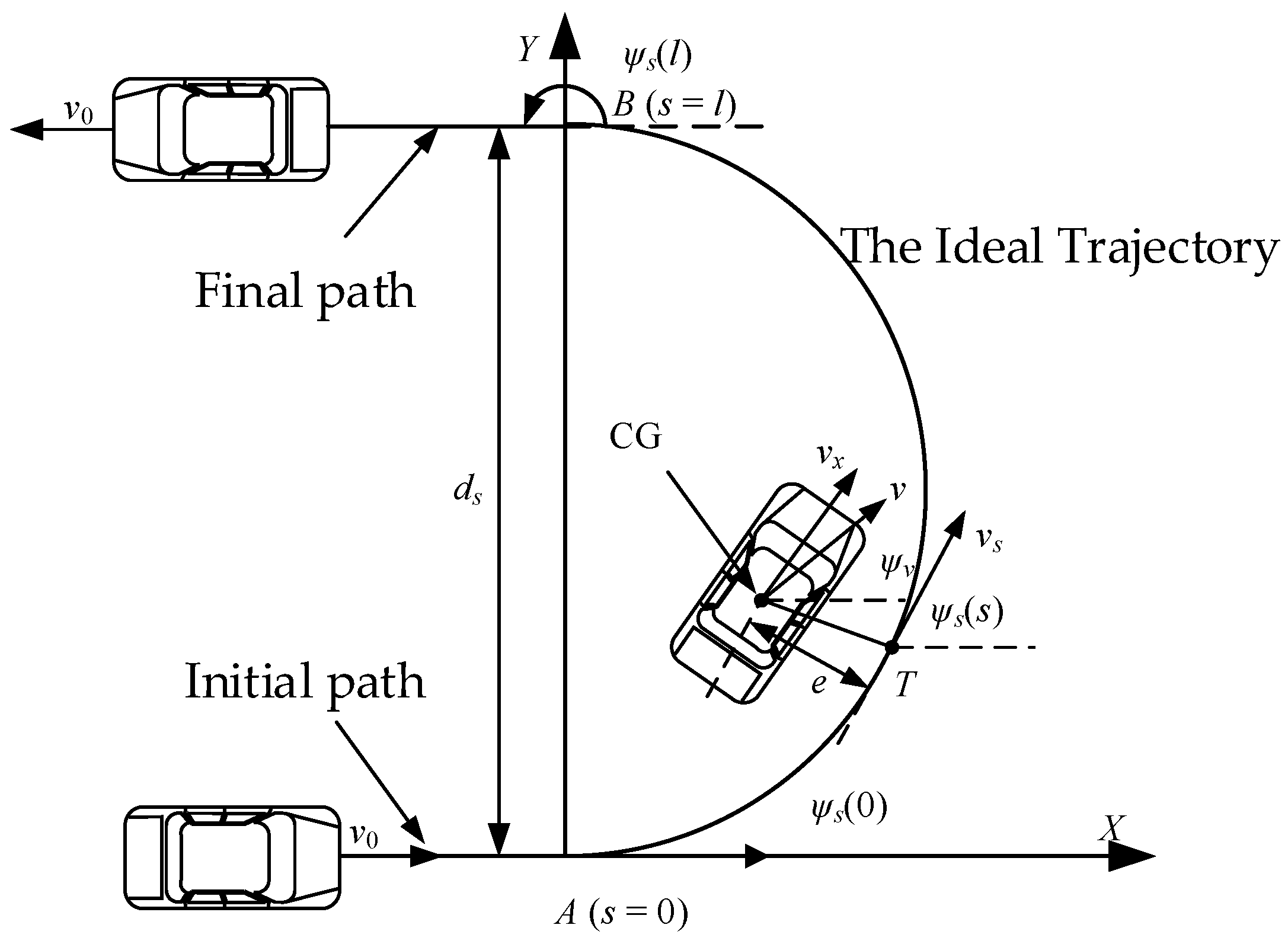
2.2. Problem Formulation

In the vehicle dynamic system, the sideslip angle is the angle between the heading direction of the vehicle and the direction of the actual velocity, and the angle of the sideslip angle is generally small because of v_x $\gg$ v_y. Therefore, the lateral velocity and lateral acceleration can be simplified as follows:

$$\left\{\begin{array}{l}{v}_y=v_x\beta \\ {\dot{v}}_y={\dot{v}}_x\beta +v_x\dot{\beta }\end{array}\right.$$

(9)

The total torque T_a = T₁ + T₂ + T₃ + T₄. Substituting (4), (8), and (9) into (1)–(3) yields the equation of the velocity. The sideslip angle and the angular velocity of the transverse pendulum are given as follows:

$${\dot{v}}_x=T_a/(mR)+d_v$$

(10)

$$\dot{\beta }=(-1+\frac{c_r-c_f}{m{v_x}^2})\gamma -\frac{c_f+c_r}{m{v}_x}\beta +\frac{c_f}{m{v}_x}{\delta }_f+d_{\beta }$$

(11)

$$\dot{\gamma }=-\frac{{l_f}^2{c}_f-{l_r}^2{c}_r}{v_{x}Iz}\gamma -\frac{l_f{c}_f-l_r{c}_r}{Iz}\beta +\frac{l_f{c}_f}{Iz}{\delta }_f+d_{\gamma }$$

(12)

where d_v, d_β, and d_γ are the unmodeled and perturbed terms.

From (10)–(12), we can deduce that the vehicle’s sideslip angle and yaw rate can be controlled by adjusting δ_f, which can effectively reduce the complexity of control. By approximating the ideal trajectory through the position and the heading angle of the intelligent vehicle, the complex trajectory tracking control is simplified into the distance error and direction error, and then the tracking control of the designed path is realized.

Figure 2 shows a model for controlling an autonomous vehicle traveling along a reference path in the Serret–Frenet framework. As shown in Figure 2, the vehicle travels along the original straight lane at a constant speed v₀ and then switches to another straight lane. A and B are the entrance and exit points of the transition path, respectively, and d_s is the distance between them.

When the vehicle enters the desired transition path, as shown in Figure 2, ψ is the directional error between the direction of the vehicle’s actual velocity ψ_v and the direction of the tangent to the desired path ψ_s, where ψ_v is expressed as follows:

$${\psi }_v=\beta +{\displaystyle {\int }_{t_0}^{t_1}\gamma dt}$$

(13)

The distance error from the orthogonal projection point T on the desired path to the vehicle’s center of gravity G is e. The equivalent tangential velocity of the vehicle along the path, v_s, which is the tangential velocity at the point in the relationship between v_s and the actual velocity of the vehicle, v, is given as follows:

$$v_s=\dot{s}=\frac{1}{1-e\kappa (s)}\left(v_x\cos \psi -v_y\sin \psi \right)\approx \frac{v_x}{1-e\kappa (s)}$$

(14)

where κ(s) is the curvature at the arc length s.

By coordinate transformation, the trajectory tracking errors of the vehicle in the Serret–Frenet framework is obtained as follows:

$$\left\{\begin{array}{l}\dot{e}=v_x\sin \psi +v_y\cos \psi \approx v_x\psi +v_x\beta \\ \dot{\psi }={\dot{\psi }}_v-{\dot{\psi }}_s\approx \gamma -\kappa v_x+\dot{\beta }\end{array}\right.$$

(15)

To consider the distance error e and the direction error ψ at the same time, the preview error (preview error) σ can be established as follows:

$$\sigma =e+L\psi$$

(16)

where L is a weighting factor reflecting the share of the directional error ψ.

Deriving (16) and combining it with (15) yields the following:

$$\dot{\sigma }=v_x\left(\psi +\beta -\kappa \right)+L\left(\gamma +\dot{\beta }\right)$$

(17)

Combining (11) and (12) for the second-order differential equation of (16), we obtain the following:

$$\ddot{\sigma }=F_v+F_{\gamma }\gamma +F_{\beta }\beta +b{\delta }_f+d_{\sigma }$$

(18)

where $F_v=\left(\psi +\beta -\kappa \right){\dot{v}}_x-\left(\kappa +\frac{d\kappa }{ds}\frac{1}{1-e\kappa }\right)v_x^2$

$$F_{\gamma }=-v_x+2\left(c_r{l}_r-c_f{l}_f\right)/\left(m{v}_x\right)-L\left({l_f}^2{c}_f+{l_r}^2{c}_r\right)/\left(v_x{I}_z\right)$$

$$F_{\beta }=-2\left(c_f+c_r\right)/m-L\left(l_f{c}_f-l_r{c}_r\right)/I_z$$

$$b=2c_f/m+L{l}_f{c}_f/I_z$$

$$d_{\sigma }=2v_x{d}_{\beta }+L{d}_{\gamma }+L\ddot{\beta }$$

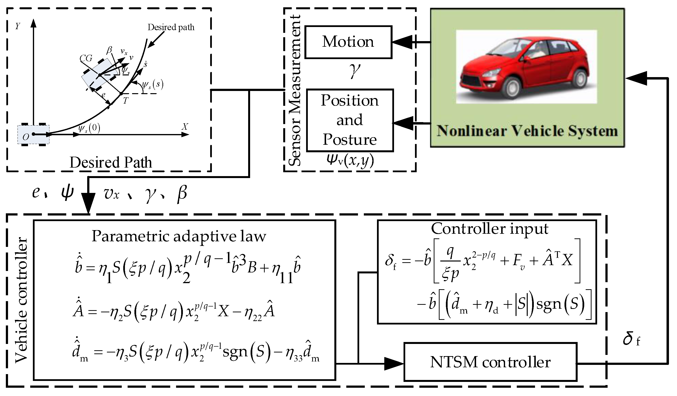
3. Trajectory Tracking Controller Design

3.1. Controller with the Known Vehicle Parameters

The controller design for the case where the vehicle parameters are known is carried out first. In this subsection, the trajectory tracking errors e and ψ can be calculated, and the longitudinal velocity v_x, the sideslip angle β, the longitudinal acceleration a_x, and the yaw rate of the vehicle γ can be measured by the inertial sensors. Therefore, e, ψ, v_x, β, a_x, and γ are known state quantities in this study.

In addition, it is assumed that the parameters m, c_f, c_r, l_f, l_r, and I_z are known in the vehicle dynamics model, while the disturbances are upper-bounded and in a known state. The second-order nonlinear system with preview error is established as follows:

$$\left\{\begin{array}{l}{\dot{x}}_1=x_2\\ {\dot{x}}_2=\ddot{\sigma }=F_v+F_{\gamma }\gamma +F_{\beta }\beta +b{\delta }_f+d_{\sigma }\end{array}\right.$$

(19)

Lemma 1

[35]. For a nonlinear system, the system is finite-time stable if V(x) is assumed to be a smooth positive definite function ($U\subset R^n$) and f(x) is a continuous function with $V^{\prime }(x)f(x)\le -c{(V(x))}^{\alpha }$, where c > 0 and 0 < α < 1. The convergence time T_r is as follows:

$$T_r\le {[c(1-\alpha )]}^{-1}{(V(x_0))}^{1-\alpha }$$

(20)

Theorem 1.

For the second-order nonlinear system (19), design the following control law:

$${\delta }_f\left(t\right)=-\frac{1}{b}\left[\frac{q}{\xi p}{x}_2^{2-p/q}+F_v+F_{\gamma }\gamma +F_{\beta }\beta +D\mathrm{sgn}\left(S\right)\right]$$

(21)

where D = d_m + η_d + |S| and (d_m ≥ |d_σ|, η_d > 0). Then, the path following error can be finite-time converged to zero. The convergence time is estimated by the following:

$$t_1\le (\sqrt{2}/{\eta }_d){(V(x_0))}^{1/2}+{\xi }^{q/p}p/\left(p-q\right)x_1{(t_0)}^{1-q/p}$$

(22)

Proof. 

To make the tracking error converge quickly and avoid the singularity problem effectively, the following non-singular terminal sliding surface is chosen as follows:

$$S\left(t\right)=x_1(t)+\xi x_2^{p/q}(t)$$

(23)

where ξ > 0, p, q are odd, 1 < p/q < 2, and all are adjustable parameters. For convenience in subsequent calculations, we will abbreviate x₁(t) and x₂(t) as x₁ and x₂, respectively. □

The Lyapunov function is selected as follows:

$$V_1\left(t\right)=(1/2)S^2\left(t\right)$$

(24)

Differentiating (24) and substituting the control input (21) yields

$$\begin{array}{ll}{\dot{V}}_1\left(t\right)& =S\left(t\right)\dot{S}\left(t\right)=S\left[{\dot{x}}_1+(\xi p/q)x_2^{p/q-1}{\dot{x}}_2\right]\\ & =-(\xi p/q)x_2^{p/q-1}\left({\eta }_d\left|S\right|+S^2\right)\\ & \le -\sqrt{2}{\eta }_d\frac{\xi p}{q}{x}_2^{p/q-1}{V}_1^{1/2}\end{array}$$

(25)

When the sliding mode S ≠ 0, the sliding mode arrival condition is satisfied since p and q are odd and 1 < p/q < 2. Therefore, the system is reaching the terminal sliding mode surface.

According to Lemma 1, the system reaches the sliding mode surface from any initial state x(0) in finite time, and the finite convergence time t_r is

$$t_r\le (\sqrt{2}/{\eta }_d){(V(x_0))}^{1/2}$$

(26)

At the sliding mold surface S = 0, the system can be expressed as follows:

$${\dot{x}}_1=-{\xi }^{-q/p}{x}_1^{q/p}$$

(27)

Establishing the Lyapunov function $V_2=(1/2)x_1^2$, the differential function of V₂ is as follows:

$${\dot{V}}_2=x_1{\dot{x}}_1=-{\xi }^{-q/p}{x}_1^{1+q/p}\le 0$$

(28)

From the above equation, we know that x₁ can converge to zero in finite time, so it can be obtained that x₂ also converges to zero in finite time. By solving (27), the time for the system to converge to the origin along the sliding mode surface S = 0 is as follows:

$$t_s={\xi }^{q/p}\frac{p}{p-q}{x}_1{(t_0)}^{1-q/p}$$

(29)

By calculating the time of the system in the two phases of converging and sliding motions (26) and (29), it is seen that the non-singular terminal sliding mode controller allows the system to converge to the origin in finite time (t_r + t_s) from any initial state. This proof is completed.

3.2. Controller with the Unknown Vehicle Parameters

As numerous vehicle parameters are practically unknown during vehicle motion, adaptive estimations of some parameters are required when designing the controller so that the control effect is always effective. F_δ, F_γ, F_β, b, and d_m in Equation (19) are usually not available in real time, and an adaptive estimation of them is required. The proof is completed.

The second-order nonlinear system (19) is first organized to obtain the following:

$$\left\{\begin{array}{l}{\dot{x}}_1=x_2\\ {\dot{x}}_2=\ddot{\sigma }=F_v+A^{T}X+b{\delta }_f+d_{\sigma }\end{array}\right.$$

(30)

where $A^T=\left[F_{\gamma } F_{\beta }\right],X^T=\left[\gamma \beta \right]$.

Lemma 2

[36]. For a nonlinear system, if there exists a continuous function V(x) and real numbers λ₁ > 0, λ₂ > 0, 0 < γ < 1, and 0 < ε < ∞ such that

$$\dot{V}(x)+{\lambda }_{1}V(x)+{\lambda }_2{V}^{\gamma }(x)+\epsilon \le 0$$

(31)

then the system is finite-time stabilized, and the residual set is given by

$$\overline{V}=\min \left\{\epsilon {\left[(1-{\theta }_0){\lambda }_2\right]}^{-1},{\epsilon }^2{\left[(1-{\theta }_0){\lambda }_2\right]}^{-2}\right\}$$

(32)

where the setup time is bounded as follows:

$$\begin{array}{r}{T}_c\le \max \left\{t_0+\frac{2}{{\theta }_0{\lambda }_1}\ln \frac{{\theta }_0{\zeta }_1{V}^{1/2}(t_0)+{\zeta }_2}{{\lambda }_2}\right.,\\ \left.t_0+\frac{2}{{\lambda }_1}\ln \frac{{\zeta }_1{V}^{1/2}(t_0)+{\theta }_0{\lambda }_2}{{\theta }_0{\lambda }_2}\right\}\end{array}$$

(33)

Theorem 2.

For a second-order nonlinear system (30), choose a non-singular terminal sliding surface (23) and design the following control law with adaptive parameters as follows:

$${\delta }_f=-\widehat{b}\left[\frac{q}{\xi p}{x}_2^{2-p/q}+F_v+{\widehat{A}}^{T}X+\left({\widehat{d}}_m+{\eta }_d+\left|S\right|\right)\mathrm{sgn}\left(S\right)\right]$$

(34)

updated the following adaptive laws as follows:

$$\left\{\begin{array}{l}\dot{\widehat{b}}={\eta }_{1}S\left(\xi p/q\right)x_2^{p/q-1}{\widehat{b}}^{3}B+{\eta }_{11}\widehat{b}\\ \dot{\widehat{A}}=-{\eta }_{2}S\left(\xi p/q\right)x_2^{p/q-1}X-{\eta }_{22}\widehat{A}\\ {\dot{\widehat{d}}}_m=-{\eta }_{3}S\left(\xi p/q\right)x_2^{p/q-1}\mathrm{sgn}\left(S\right)-{\eta }_{33}{\widehat{d}}_m\end{array}\right.$$

(35)

where $B=\frac{q}{\xi p}{x}_2^{2-p/q}+F_v+{\widehat{A}}^{T}X+\left({\widehat{d}}_m+{\eta }_d+\left|S\right|\right)\mathrm{sgn}\left(S\right)$ η₁, η₂, η₃, η₁₁, η₂₂, and η₃₃ are all positive constants, then the sliding mold surface S can converge to within the domain of the origin in finite time (t_c + t_m).

Proof. 

Define the following Lyapunov function V₃:

$$V_3=\frac{1}{2}{S}^2+\frac{1}{2{\eta }_1}{\tilde{b}}^2+\frac{1}{2{\eta }_2}{\tilde{A}}^T\tilde{A}+\frac{1}{2{\eta }_3}{\tilde{d}}_m^2$$

(36)

where $\tilde{A}=\widehat{A}-A, \tilde{b}={\widehat{b}}^{-1}-b, {\tilde{d}}_m={\widehat{d}}_m-d_m$. □

Differentiating V₃ and bringing in the controller (34) yields

$$\begin{array}{ll}{\dot{V}}_3& =S\dot{S}-{\eta }_1^{-1}{\widehat{b}}^{-2}\dot{\widehat{b}}\tilde{b}+{\eta }_2^{-1}{\tilde{A}}^T\dot{\widehat{A}}+{\eta }_3^{-1}{\dot{\widehat{d}}}_m{\tilde{d}}_m\\ & =-{\eta }_a{S}^2-{\eta }_b\left|S\right|-{\eta }_{11}^{-1}\tilde{b}{\widehat{b}}^{-1}-{\eta }_{22}^{-1}{\tilde{A}}^T\widehat{A}-{\eta }_{33}^{-1}{\tilde{d}}_m{\widehat{d}}_m\\ & =-{\eta }_a{S}^2-{\eta }_b\left|S\right|-{\eta }_{11}^{-1}\tilde{b}\left(\tilde{b}+b\right)-{\eta }_{22}^{-1}{\tilde{A}}^T\left(\tilde{A}+A\right)-\\ & \hspace{1em}{\eta }_{33}^{-1}{\tilde{d}}_m\left({\tilde{d}}_m+d_m\right)\\ & \le -{\zeta }_1{V}_2-{\zeta }_2{V_2}^{1/2}+C\end{array}$$

(37)

where ζ₁, ζ₂, and C are denoted by the following:

$${\zeta }_1=2\min \left({\eta }_a,\frac{1}{4{\eta }_{11}},\frac{1}{4{\eta }_{22}},\frac{1}{4{\eta }_{33}}\right)$$

(38)

$${\zeta }_2=2\min \left({\eta }_b,\frac{\sqrt{{\eta }_1}}{4{\eta }_{11}},\frac{\sqrt{{\eta }_2}}{4{\eta }_{22}},\frac{\sqrt{{\eta }_3}}{4{\eta }_{33}}\right)$$

(39)

$$C=\frac{1}{2{\eta }_{11}}{b}^2+\frac{1}{2{\eta }_{22}}{A}^{T}A+\frac{1}{2{\eta }_{33}}{d}_m^2+\frac{1}{4{\eta }_{11}}+\frac{1}{4{\eta }_{22}}+\frac{1}{4{\eta }_{33}}$$

(40)

With reference to Lemma 2, it follows that there exists a scalar such that V₃ converges in finite time to the following field:

$$V_3(x)\le \overline{V}=\min \left\{\frac{C}{(1-{\theta }_0){\zeta }_2},{\left(\frac{C}{(1-{\theta }_0){\zeta }_2}\right)}^2\right\},\forall t\ge t_c$$

(41)

where t_c is the set value and its value is as follows:

$$t_c\le \max \left\{t_0+\frac{2}{{\theta }_0{\zeta }_1}\ln \frac{{\theta }_0{\zeta }_1{V_2}^{1/2}(t_0)+{\zeta }_2}{{\zeta }_2}\right.,\left.t_0+\frac{2}{{\zeta }_1}\ln \frac{{\zeta }_1{V_2}^{1/2}(t_0)+{\theta }_0{\zeta }_2}{{\theta }_0{\zeta }_2}\right\}$$

(42)

Therefore, by means of the control laws (21) and the parameter adaptive laws (35), the sliding mode surface S can converge in finite time t_c within the definable interval ε (ε > 0).

After the sliding mode surface |S| converges into the interval ε, if |x₁| > ε, the Lyapunov function is established, and the differential function of V₄ is as follows:

$${\dot{V}}_4=x_1{\dot{x}}_1={\xi }^{-q/p}{x_1}^{1+q/p}{(S/x_1-1)}^{q/p}<0$$

(43)

From the above equation, we know that |x₁| can converge to within the interval ε in finite time which means that the error can converge to within the interval ε in finite time. The time to converge to within the interval is given by the calculation of

$$t_m\le \left\{\begin{array}{l}{\xi }^{q/p}{\left(1-q/p\right)}^{-1}{(x_1(t_0)-\epsilon )}^{1-q/p},\hspace{1em}{x}_1(t_0)>\epsilon \\ {\xi }^{q/p}{\left(1-q/p\right)}^{-1}{(x_1(t_0)+\epsilon )}^{1-q/p},\hspace{1em}{x}_1(t_0)<-\epsilon \end{array}\right.$$

(44)

By calculating the time (42) and (44) of the system in both the converging and sliding motion phases, we can see that the non-singular terminal sliding mode controller allows the system to converge from an arbitrary initial state for a finite time (t_c + t_m) into the definable interval ε. This completes the proof.

Remark 1.

Building upon the proof process outlined above, the designed controller will induce the error to converge to a very minimal range in a fixed amount of time, a feature particularly beneficial in practical applications. Integrating the NTSM with an adaptive algorithm can effectively suppress a large chattering phenomenon and deal with the work condition in which environment parameters are unknown.

4. Simulation Analysis

To show the effectiveness of the proposed control strategy, the simulation studies under real operating conditions with uncertainties and perturbations are implemented on the CarSim–Matlab platform. Then, validate the effectiveness of the controller using a U-turn trajectory. The U-turn trajectory includes both straight and curved segments, and by switching between these trajectories while the vehicle is in motion, a more comprehensive validation of the controller’s effectiveness can be achieved.

The results of the CarSim–Matlab joint simulation platform are shown in Figure 3, and the nonlinear dynamic vehicle model and real road conditions are included in CarSim. The parameter adaptive controller in Theorem 2 enables the control parameters to change with the working conditions; finally, the NTSM controller calculates the front wheel angle to realize that the vehicle can track the ideal transition path with uncertain parameters.

After the system reaches the sliding mode surface, ideally it needs to generate infinite frequency switching control to maintain the sliding mode of the system, so the chattering phenomenon cannot be avoided; in this paper, the controller adopts the saturation function sat(x) instead of the sign function sgn(x) to reduce the chattering phenomenon. The sat(x) function is defined as follows:

$$\mathit{sat}(x)=\left\{\begin{array}{l}1, x>{\left(k_{sat}\right)}^{-1}\\ x\times k_{sat}, -{\left(k_{sat}\right)}^{-1}<x<{\left(k_{sat}\right)}^{-1}\\ -1, x<-{\left(k_{sat}\right)}^{-1}\end{array}\right.$$

(45)

The physical parameters of the vehicle in the simulation are shown in

Table 2. Vehicle model parameters.

Parameter	Value	Parameter	Value
m	1230 kg	IZ	1343 kg·m2
lf	1.04 m	cf	96,300 N/rad
lr	1.56 m	cr	64,200 N/rad
d	1.48 m	g	9.8 m/s2
R	0.3 m	vd	50 km/h

. The parameters of the controllers (34) and (35) are selected, as shown in

Table 3. Controllers’ parameters.

Controllers	Parameter
Sliding mold surface (22)	ξ = 0.4, p = 7, q = 5
Adaptive control laws, (40)	η1 = 0.4, η11 = 0.08, η2 = [0.5 1], η22 = [1 0.5], η3 = 5, η33 = 2
NTSM controllers, (39)	ηd = 5, L = 1.4, ksat = 8

. The data in Table 2 represent the standard parameters of the B-class vehicle model in the CarSim platform, provided by the CarSim platform itself.

The smooth path with continuous curvature facilitates the vehicle to make continuous steering inputs, and curves such as the equal-radius arc, cubic helix, and gyratory line are generally chosen as the transition paths of the path planner, among which the gyratory line path with linear curvature change has been widely used in path planning due to its simple form and continuous transition curvature. Therefore, in this paper, we refer to the gyratory line as the transition path in the literature [11].

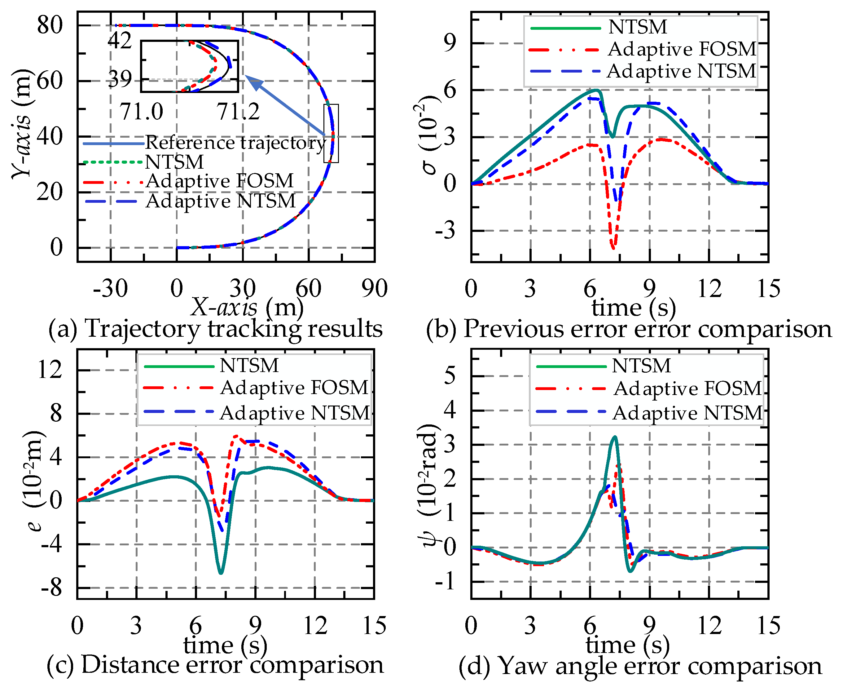
4.1. Simulation Results of Three Sliding Mode Controllers

To validate the trajectory tracking performance of the parameter-adaptive non-singular terminal sliding mode controller (adaptive NTSM), the parameter-adaptive linear sliding mode controller parameter (adaptive FOSM) is simulated with the parameter-known non-singular terminal sliding mode controller (NTSM) under the same driving conditions.

The linear sliding mode controller still uses Formulas (34) and (35) and needs to modify which p, q values are modified to 1, and the parameter-known non-singular terminal sliding mode controller needs Formula (34) in $\widehat{b}$, $\widehat{A}$, and ${\widehat{d}}_m$, with the calculation of the determination of the value instead, so that $\widehat{b}=0.15$, ${\widehat{A}}^T=[\begin{array}{cc}0.01& 0.1\end{array}]$, and ${\widehat{d}}_m=1$. The vehicle speed is 50 km/h, an ordinary asphalt pavement is selected, the pavement adhesion coefficient μ = 0.6, and the simulation results are shown in Figure 4.

The trajectory tracking performance of the three sliding mode controllers for the U-turn path is given in Figure 4. Figure 4a shows the change in the displacement of the vehicle in the y-axis direction with the displacement in the x-axis direction under the inertial coordinate system, and it can be seen from the figure that all three sliding mode controllers can track the ideal trajectory well, but the parameter-adaptive NTSM controller has the best tracking performance. Figure 4b shows the preview error variation process of trajectory tracking control; as shown in the figure, all three controllers meet the requirements. Figure 4c,d show the changes in the distance error and yaw angle error with time in the three controllers, respectively, and the maximum absolute value of error of the parameter-adaptive non-singular terminal sliding mode controller is smaller than the remaining two controllers, so the tracking accuracy of the parameter-adaptive non-singular terminal sliding mode controller is optimal among the three controllers. In summary, all three controllers can guarantee the vehicle tracking reference path, and the tracking accuracy of the parameter-adaptive non-singular terminal sliding mode controller is higher.

4.2. Robustness of Non-Singular Terminal Sliding Mode with Parameter Adaptation

To analyze the feasibility of the proposed control algorithm more comprehensively, several different simulation conditions are designed here to simulate the actual driving environment.

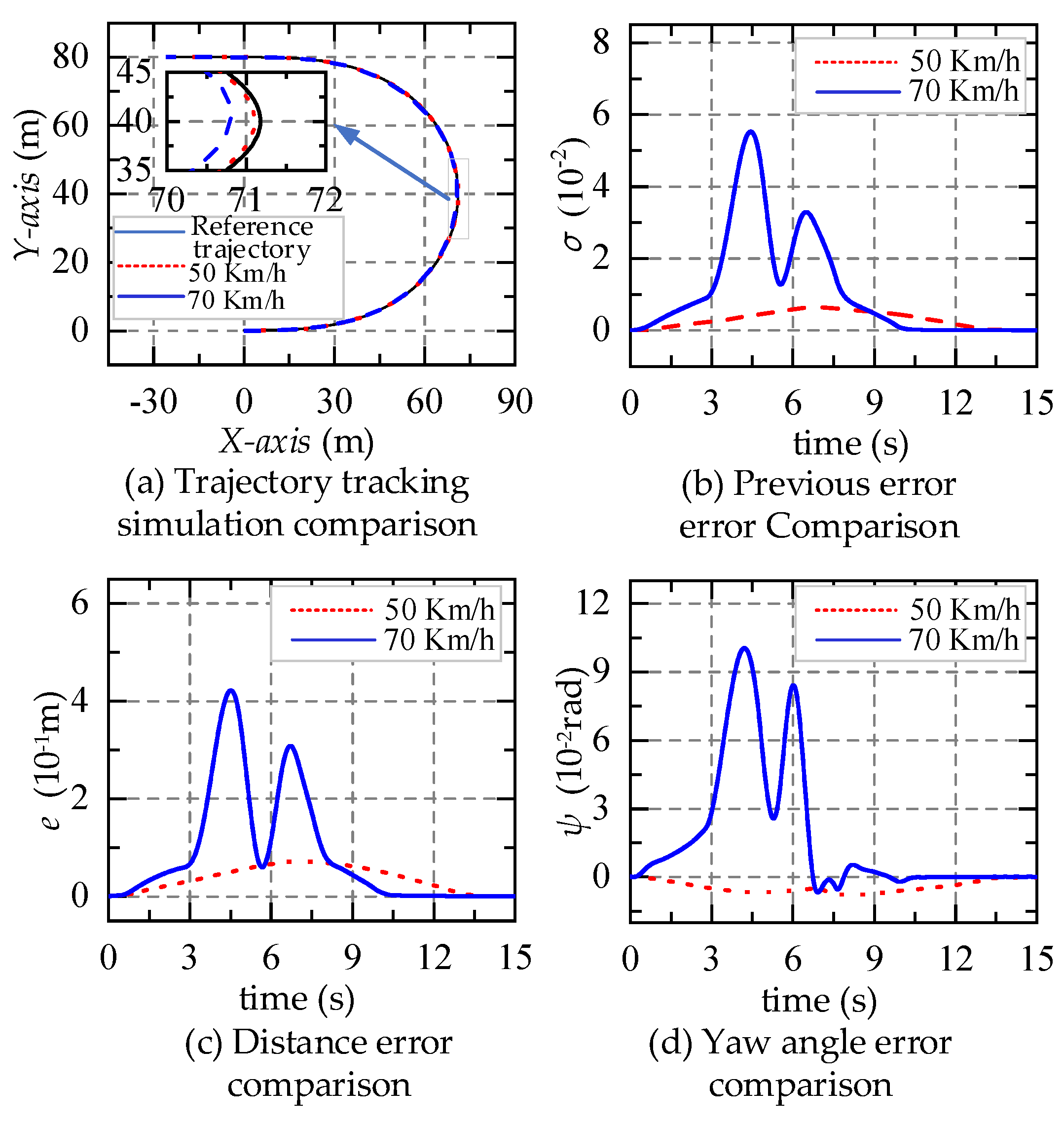
4.2.1. Robustness to Vehicle Speed

Unlike some controllers, the NTSM controller with parameter adaptation does not need to set different control parameters for different vehicle speeds, and it is robust to changes in vehicle speeds, mainly because the parameter adaptive control law is able to dynamically estimate and compensate for the total perturbation of the system, to verify the performance. The controller uses the same control parameters, the vehicle speed is set to two speeds 50 km/h and 70 km/h, the driving surface is selected to be a dry concrete road, and the coefficient of adhesion μ = 0.7.

The simulation results are shown in Figure 5. As shown in the figure, the vehicle has good trajectory tracking performance at different speeds under the same control parameters, demonstrating the good robustness of the parameter-adaptive non-singular terminal sliding mode controller to speed. Meanwhile, the vehicle’s trajectory tracking accuracy is high when the vehicle speed is low, which is mainly because that with the increase in the vehicle speed, when the vehicle turns at a large angle, the vehicle tires may enter the nonlinear region, and there is a large error in the vehicle model. Based on the above analysis, this controller can make the vehicle follow the reference path well at different speeds.

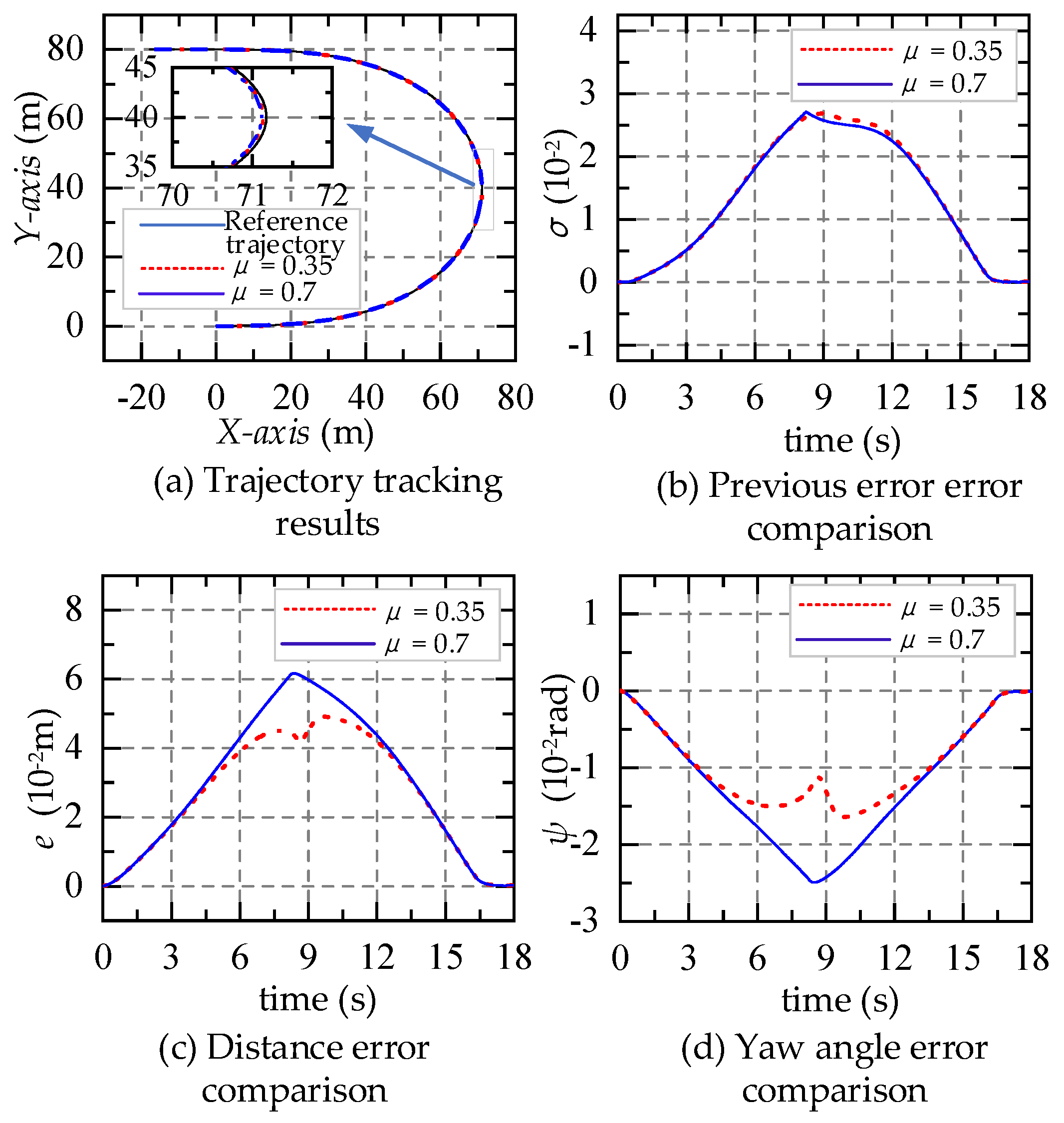
4.2.2. Robustness to Road Adhesion Coefficients

When the vehicle is driven under different road conditions, the dynamic parameters (e.g., tire lateral deflection stiffness) change, which challenges the performance of the controller. The road adhesion coefficients μ = 0.35 and 0.7 are chosen to represent rainy and snowy road surfaces and dry concrete road surfaces, respectively, and the speed of the vehicle is 40 km/h.

The trajectory tracking performance of the NTSM controller for different road surface attachment coefficients is shown in Figure 6. The non-singular terminal sliding mode controller with parameter adaption enables the vehicle to follow the reference path well on the road surface with different adhesion conditions. Even though the saturation situation of the tire lateral force occurs under large angle steering conditions, the trajectory tracking controller can correct the deviation in time so that the deviation converges to zero.

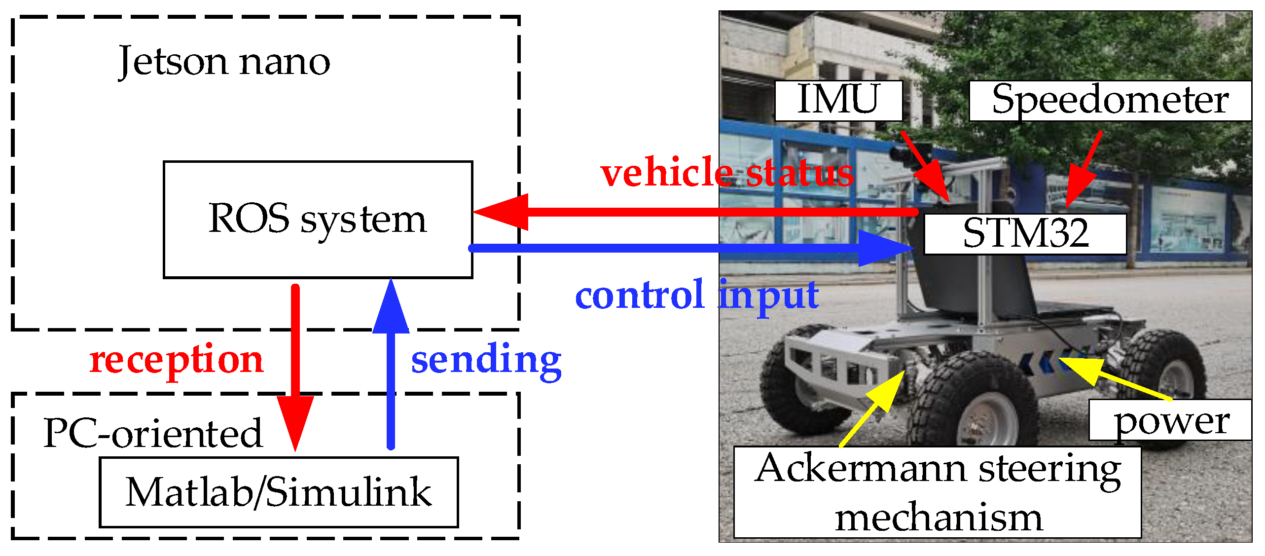
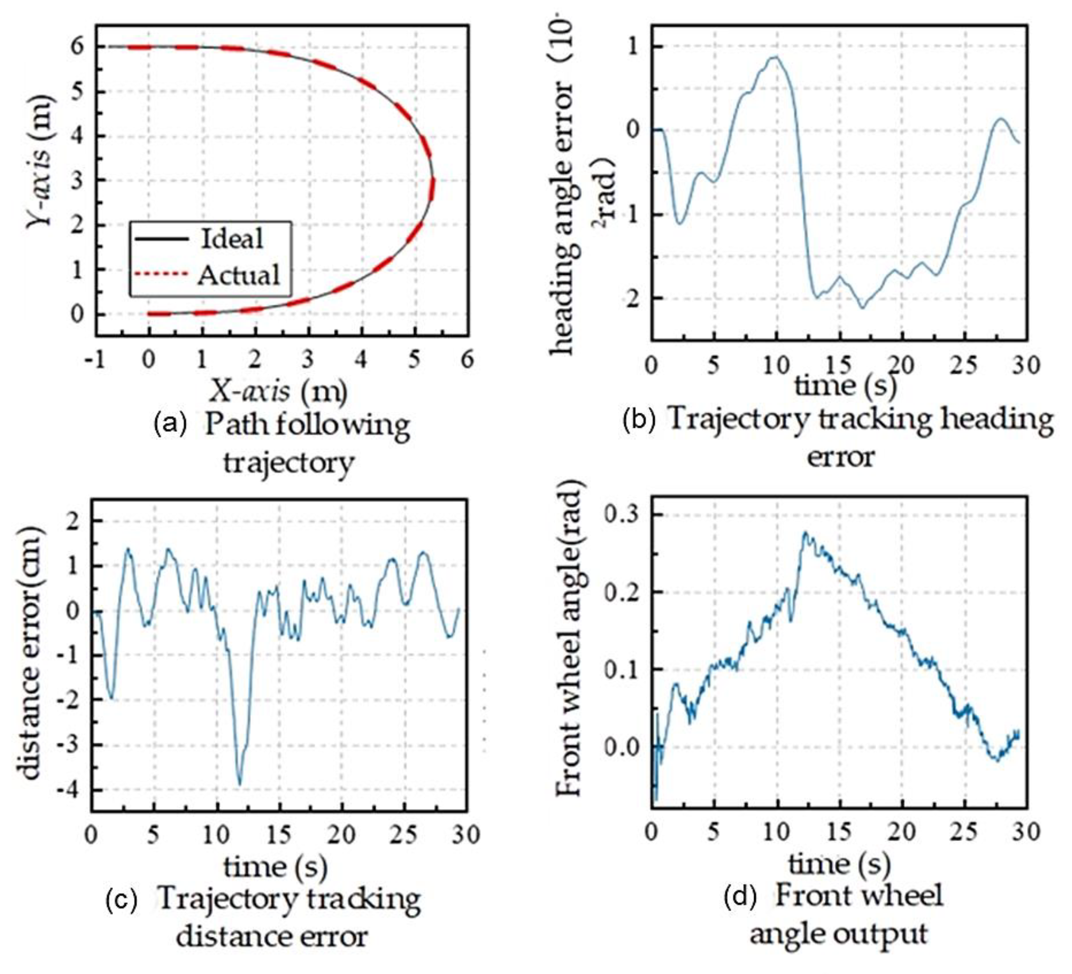
5. Experimental Verification of Trajectory Tracking Controller

The experimental platform used in this paper is a front-wheel Ackermann steering autonomous vehicle developed based on the ROS system, and the experimental platform can be divided into three layers at the hardware level: the PC side, the Jetson Nano (upper computer), and the STM32 core board (lower computer); the PC side is equipped with the Windows system, and the controller in Simulink outputs the control quantities to the core board through the ROS system and receives the core board to send the sensor signals to realize the closed-loop control of the system (see Figure 7).

STM32 serves as the underlying control board, capable of collecting data from sensors such as the IMU and odometers via serial communication and providing feedback to the corresponding ROS nodes. The Jetson Nano can directly connect to the underlying STM32 control board to receive vehicle status information or send control commands.

Algorithm Experimental Validation Results

In this subsection, the sensor information of the autonomous vehicle is passed into Matlab–Simulink to compute the trajectory of the vehicle, and the next front wheel angle of the vehicle is computed according to the ideal trajectory using the NTSM controller to realize the trajectory tracking control of the unmanned vehicle.

When applying the trajectory tracking controller, the actual physical parameters of the unmanned vehicle are required for the tracking controller. After measurement, we obtain its size as shown in the

Table 4. Vehicle parameters.

Parameter	Value	Parameter	Value
m	35.16 kg	IZ	2.188 kg·m2
lf	0.25 m	cf	1130 N/rad
lr	0.25 m	cr	1130 N/rad
d	0.6 m	g	9.8 m/s2
R	0.128 m	vd	1.8 km/h

, and the traveling speed is chosen as 0.5 m/s.

The goal of intelligent vehicle trajectory tracking control is to track the desired path provided by path planning. A smooth gyratory path with continuous curvature is more convenient for the vehicle to perform continuous steering inputs, and the tracking results are shown in Figure 8.

Figure 8 shows the tracking performance of the trajectory tracking controllers for the U-turn path of the gyratory line. Figure 8a demonstrates the variation in the vehicle’s displacement in the y-axis direction with the displacement in the x-axis direction under the inertial coordinate system, and it can be seen from the figure that the NTSM controllers are all able to track the ideal trajectory very well. The ideal trajectory and the actual trajectory in the figure are essentially in close alignment. Figure 8b,c show the variation in the heading angle error and distance error with time during trajectory tracking, respectively. The error in the heading angle of the vehicle shown in the figure stabilizes within a range of 10⁻² rad. The error between the actual trajectory and the ideal trajectory does not exceed 4 cm. Both errors fluctuate within a small range. The smaller error indicates that the controller performs very well. Figure 8d shows the output value of the front wheel steering during trajectory tracking, and from the figure, the corner change during the control process is smooth with no corner mutation. In summary, the NTSM controller can ensure that the unmanned vehicle can track the reference path with high accuracy, and the whole control process is relatively smooth, which meets the design requirements.

6. Conclusions

This paper discusses the trajectory tracking problem of intelligent vehicles and proposes a control strategy with high trajectory tracking accuracy and robustness. The vehicle’s trajectory tracking error in the Serret–Frenet framework is first obtained. This article carries out the design of a non-singular terminal sliding mode controller with known control parameters. The sliding mode is employed to ensure the high robustness of the controller. In addition, the sliding mode control method can not only ensure the high robustness but also has advantages such as insensitivity to parameter variations and perturbations, a simple physical realization. Based on this, an adaptive estimation of unknown parameters is carried out, and the design of the final controller is completed. The introduction of adaptive control methods allows us to design controllers without measuring actual external parameters, ensuring the effectiveness of the controller. The controller utilizes the adaptive control method to estimate and compensate for the unmodeled dynamic perturbations and external perturbations of the system and makes the tracking error converge to zero in a finite time. Finally, the proposed control strategy is simulated by the CarSim–Matlab simulation platform and verified by the real-vehicle experiments. The results show that the control strategy can ensure the vehicle tracks the reference path quickly and accurately with strong robustness.

References

1. Xavier, N.; Bandyopadhyay, B. Practical Sliding Mode Using State Depended Intermittent Control. IEEE Trans. Circuits Syst. II: Express Briefs 2021, 68, 341–345. [Google Scholar] [CrossRef]
2. Liang, Z.; Zhao, J.; Dong, Z.; Wang, Y.; Ding, Z. Torque Vectoring and Rear-Wheel-Steering Control for Vehicle’s Uncertain Slips on Soft and Slope Terrain Using Sliding Mode Algorithm. IEEE Trans. Veh. Technol. 2020, 69, 3805–3815. [Google Scholar] [CrossRef]
3. Nguyen, N.P.; Oh, H.; Moon, J. Continuous Nonsingular Terminal Sliding-Mode Control With Integral-Type Sliding Surface for Disturbed Systems: Application to Attitude Control for Quadrotor UAVs Under External Disturbances. IEEE Trans. Aerosp. Electron. Syst. 2022, 58, 5635–5660. [Google Scholar] [CrossRef]
4. Guo, S.; Orosz, G.; Molnar, T.G. Connected Cruise and Traffic Control for Pairs of Connected Automated Vehicles. IEEE Trans. Intell. Transp. Syst. 2023, 24, 12648–12658. [Google Scholar] [CrossRef]
5. Chen, X.; Xu, B.; Qin, X.; Bian, Y.; Hu, M.; Sun, N. Non-Signalized Intersection Network Management With Connected and Automated Vehicles. IEEE Access 2020, 8, 122065–122077. [Google Scholar] [CrossRef]
6. Qin, Z.; Chen, L.; Fan, J.; Xu, B.; Hu, M.; Chen, X. An Improved Real-Time Slip Model Identification Method for Autonomous Tracked Vehicles Using Forward Trajectory Prediction Compensation. IEEE Trans. Instrum. Meas. 2021, 70, 7501012. [Google Scholar] [CrossRef]
7. Subroto, R.K.; Wang, C.Z.; Lian, K.L. Four-Wheel Independent Drive Electric Vehicle Stability Control Using Novel Adaptive Sliding Mode Control. IEEE Trans. Ind. Appl. 2020, 56, 5995–6006. [Google Scholar] [CrossRef]
8. Wen, S.; Guo, G. Distributed Trajectory Optimization and Sliding Mode Control of Heterogenous Vehicular Platoons. IEEE Trans. Intell. Transp. Syst. 2022, 23, 7096–7111. [Google Scholar] [CrossRef]
9. Ge, X.; Han, Q.-L.; Wu, Q.; Zhang, X.-M. Resilient and Safe Platooning Control of Connected Automated Vehicles Against Intermittent Denial-of-Service Attacks. IEEE/CAA J. Autom. Sin. 2023, 10, 1234–1251. [Google Scholar] [CrossRef]
10. Wang, B.; Su, R. A Distributed Platoon Control Framework for Connected Automated Vehicles in an Urban Traffic Network. IEEE Trans. Control Netw. Syst. 2022, 9, 1717–1730. [Google Scholar] [CrossRef]
11. Scheffe, P.; Henneken, T.M.; Kloock, M.; Alrifaee, B. Sequential Convex Programming Methods for Real-Time Optimal Trajectory Planning in Autonomous Vehicle Racing. IEEE Trans. Intell. Veh. 2023, 8, 661–672. [Google Scholar] [CrossRef]
12. Ju, Z.; Zhang, H.; Li, X.; Chen, X.; Han, J.; Yang, M. A Survey on Attack Detection and Resilience for Connected and Automated Vehicles: From Vehicle Dynamics and Control Perspective. IEEE Trans. Intell. Veh. 2022, 7, 815–837. [Google Scholar] [CrossRef]
13. Tang, L.; Yan, F.; Zou, B.; Wang, K.; Lv, C. An Improved Kinematic Model Predictive Control for High-Speed Path Tracking of Autonomous Vehicles. IEEE Access 2020, 8, 51400–51413. [Google Scholar] [CrossRef]
14. Wang, H.; Liu, B. Path Planning and Path Tracking for Collision Avoidance of Autonomous Ground Vehicles. IEEE Syst. J. 2022, 16, 3658–3667. [Google Scholar] [CrossRef]
15. Hu, C.; Chen, Y.; Wang, J. Fuzzy Observer-Based Transitional Path-Tracking Control for Autonomous Vehicles. IEEE Trans. Intell. Transp. Syst. 2021, 22, 3078–3088. [Google Scholar] [CrossRef]
16. Guan, Y.; Ren, Y.; Li, S.E.; Sun, Q.; Luo, L.; Li, K. Centralized Cooperation for Connected and Automated Vehicles at Intersections by Proximal Policy Optimization. in IEEE Trans. Veh. Technol. 2020, 69, 12597–12608. [Google Scholar] [CrossRef]
17. Bai, W.; Xu, B.; Liu, H.; Qin, Y.; Xiang, C. Robust Longitudinal Distributed Model Predictive Control of Connected and Automated Vehicles With Coupled Safety Constraints. IEEE Trans. Veh. Technol. 2023, 72, 2960–2973. [Google Scholar] [CrossRef]
18. Xu, H.; Xiao, W.; Cassandras, C.G.; Zhang, Y.; Li, L. A General Framework for Decentralized Safe Optimal Control of Connected and Automated Vehicles in Multi-Lane Signal-Free Intersections. IEEE Trans. Intell. Transp. Syst. 2022, 23, 17382–17396. [Google Scholar] [CrossRef]
19. Liu, Y.; Zhou, B.; Wang, X.; Li, L.; Cheng, S.; Chen, Z.; Li, G.; Zhang, L. Dynamic Lane-Changing Trajectory Planning for Autonomous Vehicles Based on Discrete Global Trajectory. IEEE Trans. Intell. Transp. Syst. 2022, 23, 8513–8527. [Google Scholar] [CrossRef]
20. Mohamed, M.; Rabik, S.; Vasanth, T. Muthuramalingam. Implementation of LQR based SOD control in diode laser beam machining on leather specimens, Optics & Laser Technology. Automatica 2024, 170, 110328. [Google Scholar]
21. Li, Q.; Ding, B. Design of Backstepping Sliding Mode Control for a Polishing Robot Pneumatic System Based on the Extended State Observer. Machines 2023, 11, 904. [Google Scholar] [CrossRef]
22. Ye, Y.; Wang, Y.; Wang, L.; Wang, X. A modified predictive PID controller for dynamic positioning of vessels with autoregressive model. Ocean Eng. 2023, 284, 115176. [Google Scholar] [CrossRef]
23. Fu, Q.; Wu, J.; Yu, C.; Feng, T.; Zhang, N.; Zhang, J. Linear Quadratic Optimal Control with the Finite State for Suspension System. Machines 2023, 11, 127. [Google Scholar] [CrossRef]
24. Gao, Z.; Wu, Z.; Hao, W.; Long, K.; Byon, Y.-J.; Long, K. Optimal Trajectory Planning of Connected and Automated Vehicles at On-Ramp Merging Area. IEEE Trans. Intell. Transp. Syst. 2022, 23, 12675–12687. [Google Scholar] [CrossRef]
25. Chen, N.; van Arem, B.; Alkim, T.; Wang, M. A Hierarchical Model-Based Optimization Control Approach for Cooperative Merging by Connected Automated Vehicles. IEEE Trans. Intell. Transp. Syst. 2021, 22, 7712–7725. [Google Scholar] [CrossRef]
26. Kim, S.; Lee, J.; Han, K.; Choi, S.B. Vehicle Path Tracking Control Using Pure Pursuit With MPC-Based Look-Ahead Distance Optimization. IEEE Trans. Veh. Technol. 2024, 73, 53–66. [Google Scholar] [CrossRef]
27. Liang, Z.; Zhao, J.; Liu, B.; Wang, Y.; Ding, Z. Velocity-Based Path Following Control for Autonomous Vehicles to Avoid Exceeding Road Friction Limits Using Sliding Mode Method. IEEE Trans. Intell. Transp. Syst. 2020, 23, 1947–1958. [Google Scholar] [CrossRef]
28. Wu, Y.; Wang, L.; Zhang, J.; Li, F. Path Following Control of Autonomous Ground Vehicle Based on Nonsingular Terminal Sliding Mode and Active Disturbance Rejection Control. IEEE Trans. Veh. Technol. 2019, 68, 6379–6390. [Google Scholar] [CrossRef]
29. Labbadi, M.; Djemai, M.; Boubaker, S. A novel non-singular terminal sliding mode control combined with integral sliding surface for perturbed quadrotor. Proc. Inst. Mech. Eng. Part I J. Syst. Control Eng. 2022, 236, 999–1009. [Google Scholar] [CrossRef]
30. Lei, Q.; Zhang, W. Adaptive non-singular integral terminal sliding mode tracking control for autonomous underwater vehicles. IET Control Theory Appl. 2017, 11, 1293–1306. [Google Scholar]
31. Shen, H.; Pan, Y.J.; Ahmad, U.; He, B. Pose Synchronization of Multiple Networked Manipulators Using Nonsingular Terminal Sliding Mode Control. IEEE Trans. Syst. Man Cybern. Syst. 2021, 51, 12. [Google Scholar] [CrossRef]
32. Guo, J.; Luo, Y.; Li, K. An Adaptive Hierarchical Trajectory Following Control Approach of Autonomous Four-Wheel Independent Drive Electric Vehicles. IEEE Trans. Intell. Transp. Syst. 2018, 19, 2482–2492. [Google Scholar] [CrossRef]
33. Liang, Z.; Wang, Z.; Zhao, J.; Wong, P.K.; Yang, Z.; Ding, Z. Fixed-Time Prescribed Performance Path-Following Control for Autonomous Vehicle With Complete Unknown Parameters. IEEE Trans. Ind. Electron. 2023, 70, 8426–8436. [Google Scholar] [CrossRef]
34. Liang, Z.; Shen, M.; Li, Z.; Yang, J. Model-Free Output Feedback Path Following Control for Autonomous Vehicle With Prescribed Performance Independent of Initial Conditions. IEEE/ASME Trans. Mechatron. 2023, 10, 1–12. [Google Scholar] [CrossRef]
35. Ghasemi, M.; Nersesov, S.G. Finite-time coordination in multiagent systems using sliding mode control approach. Automatica 2014, 50, 1209–1216. [Google Scholar] [CrossRef]
36. Yu, J.; Shi, P.; Zhao, L. Finite-time command filtered backstepping control for a class of nonlinear systems. Automatica 2018, 92, 173–180. [Google Scholar] [CrossRef]
Figure 1. Vehicle dynamics model.
Machines 12 00237 g001
Figure 2. Trajectory tracking model.
Machines 12 00237 g002
Figure 3. Trajectory tracking algorithm framework.
Machines 12 00237 g003
Figure 4. (ad) Simulation results of three sliding mode controllers.
Machines 12 00237 g004
Figure 5. (ad) Simulation results at different speeds.
Machines 12 00237 g005
Figure 6. (ad) Simulation results under different road adhesion coefficients.
Machines 12 00237 g006
Figure 7. Experimental platform framework.
Machines 12 00237 g007
Figure 8. (ad) Experimental results of trajectory tracking.
Machines 12 00237 g008