Abstract
When faced with challenges such as adapting to dynamic environments and handling ambiguous identification, indoor service robots encounter manifold difficulties. This paper aims to address this issue by proposing the design of a service robot equipped with precise small-object recognition, autonomous path planning, and obstacle-avoidance capabilities. We conducted in-depth research on the suitability of three SLAM algorithms (GMapping, Hector-SLAM, and Cartographer) in indoor environments and explored their performance disparities. Upon this foundation, we have elected to utilize the STM32F407VET6 and Nvidia Jetson Nano B01 as our processing controllers. For the program design on the STM32 side, we are employing the FreeRTOS operating system, while for the Jetson Nano side, we are employing ROS (Robot Operating System) for program design. The robot employs a differential drive chassis, enabling successful autonomous path planning and obstacle-avoidance maneuvers. Within indoor environments, we utilized the YOLOv3 algorithm for target detection, achieving precise target identification. Through a series of simulations and real-world experiments, we validated the performance and feasibility of the robot, including mapping, navigation, and target detection functionalities. Experimental results demonstrate the robot’s outstanding performance and accuracy in indoor environments, offering users efficient service and presenting new avenues and methodologies for the development of indoor service robots.
1. Introduction
Mobile robots possess the autonomy to navigate within their designated environments. They can perceive their surroundings, execute actions according to instructions, and make decisions, thereby efficiently, effectively, and safely accomplishing tasks [1]. Various service robots have already been providing assistance across various industries, including manufacturing, warehousing, healthcare, agriculture, and hospitality [2]. Within the service industry, there is a growing trend of utilizing robots as restaurant attendants. Due to a shortage of human servers, restaurant owners have begun seeking robots to assist in customer service [3]. With the advancement of artificial intelligence technology, powerful onboard processors, ubiquitous sensors, and the development of simultaneous localization and mapping (SLAM) techniques, automated guided vehicle (AGV) systems have evolved into autonomous mobile robots (AMRs), offering greater operational flexibility and enhanced productivity [4]. In recent years, service robots have emerged as a highly active research area [5].
Following an in-depth investigation and analysis by Zhang Xiaoying and colleagues, they concluded that the rapid advancement of predictive remote control technology has opened up extensive application prospects for mobile service robots [6]. From navigation assistants in commercial retail to precise control of advanced medical devices, mobile service robots have become an indispensable part of modern society [6]. Jha Sanjay Kumar discussed the application of robots in libraries and information centers, how they are transforming library services, and speculated on the future possibilities and trends of robot utilization in libraries, while also citing current applications of robots in libraries and providing a case study of library adoption of telepresence robots. The study combined examples of libraries employing various types of robots, summarizing the scenarios where AI-mediated robots engage in various activities within libraries [7]. Scholars such as Ye Yangqing delved into the requirements for real-time accurate identification and localization of target objects in indoor settings for household service robots operating in homes and offices. This presents certain challenges for object detection, especially in scenarios involving small objects such as fruits and utensils in everyday life, making object recognition and localization more complex [8].
To address the challenges of accurate object recognition and indoor navigation, this study endeavors to research and design a service robot tailored specifically for indoor environments, aiming to resolve issues such as unclear recognition, path planning, and obstacle avoidance. In comparison to existing software and hardware solutions, the proposed method is targeted and efficient, offering effective solutions for small-object recognition and indoor path-planning challenges. The main contributions of this paper are as follows:
- Design of a specialized indoor service robot: The focus of this research is to develop an indoor service robot tailored for office environments, aimed at addressing challenges such as accurate target recognition, path planning, and obstacle avoidance. This robot is capable of accurately identifying small objects and autonomously planning paths while avoiding obstacles.
- Indoor SLAM algorithm analysis: This paper conducts an in-depth analysis of three commonly used SLAM algorithms (GMapping, Hector-SLAM, Cartographer) to assess their suitability and performance differences in indoor environments [9]. The research begins with preliminary planning through SLAM simulation experiments. Subsequently, by comparing the output results of different algorithms in experimental settings, the most suitable algorithm for application scenarios involving the robot is selected.
- Hardware and software implementation: This paper utilizes the STM32F407VET6 and Nvidia Jetson Nano B01 as the main control units. The FreeRTOS operating system is employed for program design on the STM32 side, while the ROS (Robot Operating System) is used on the Jetson Nano side. This selection maximizes the resources of the STM32F407VET6 for hardware choices. Considering the computational capabilities of the Jetson Nano B01, appropriate navigation and vision algorithms have been selected for the software implementation. For global path planning, Dijkstra’s algorithm is used, while for local path planning, the teb_local_planner algorithm is employed. In terms of visual recognition, the lightweight YOLOv3 algorithm is chosen for object detection. This configuration enables the robot to autonomously plan paths and navigate when encountering obstacles, while also ensuring precise object detection using machine vision. Ultimately, this setup guarantees efficient service provision to users by facilitating accurate navigation and object recognition.
The paper begins by introducing the overall design of the robot, including chassis design, control system design, and visual component design. In the robot design section, it focuses on discussing the differential wheel chassis design and kinematic analysis, as well as the control system design. Subsequently, it provides detailed descriptions of the experimental design and results, including SLAM simulation experiments, path planning and navigation simulation experiments, and real-world experiments in actual and office environments. Finally, it analyzes and discusses the experimental results and draws conclusions. This study aims to reduce the time cost of indoor item recognition while effectively addressing challenges of accurate object recognition and indoor navigation.
2. Robot Design
2.1. Robot Chassis Design and Kinematics Analysis
2.1.1. Differential Wheel Chassis Design
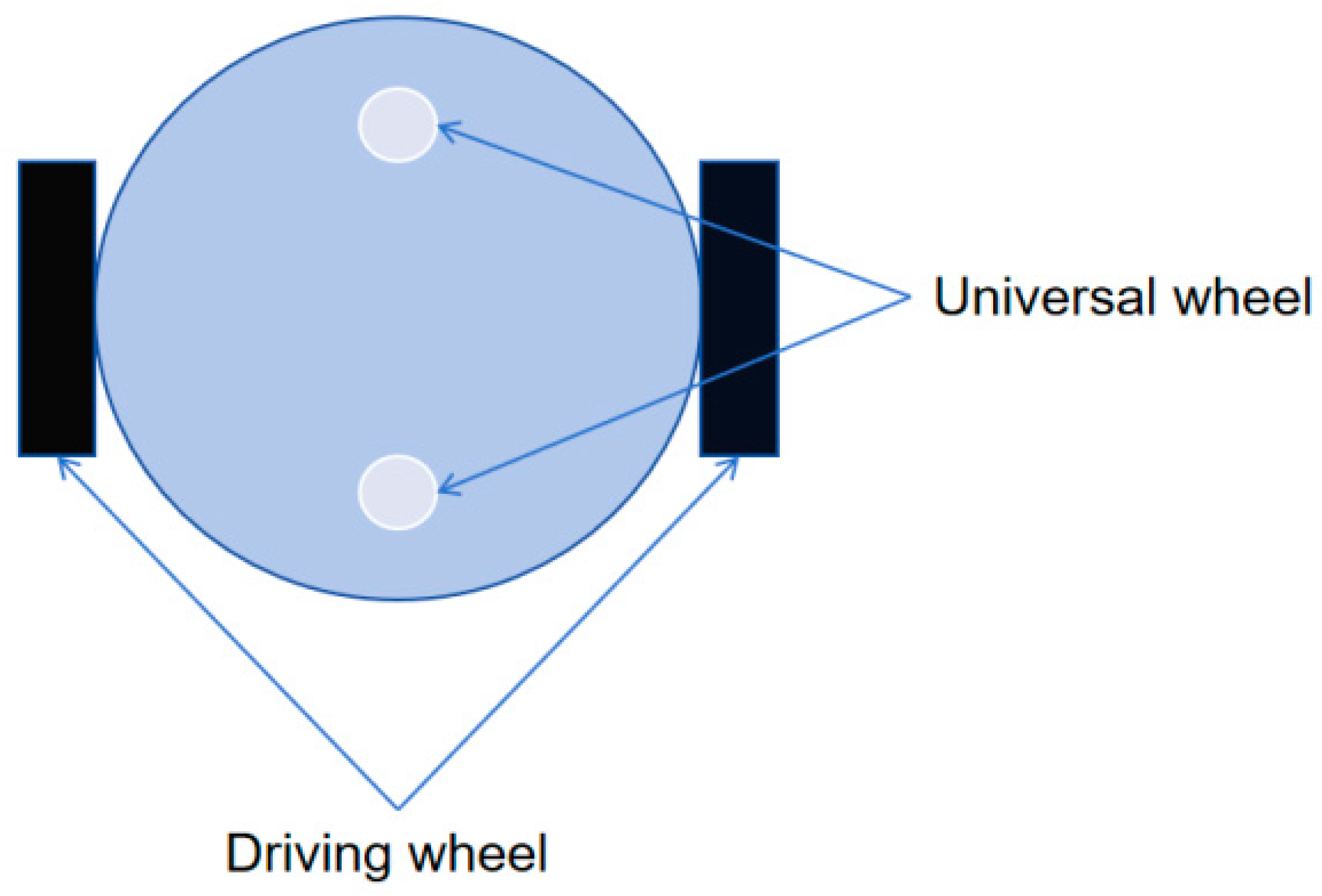
Considering the need for robots to possess the capability of flexible steering and stable motion, we have chosen to adopt a design consisting of two differential-driven wheels paired with two sets of omni-directional wheels. This layout enables the chassis to maneuver freely while maintaining stability. In this design, the two main wheels are placed on the left and right sides of the chassis, combined with two sets of omni-directional wheels, facilitating the chassis’ free steering and motion, as depicted in Figure 1. Additionally, through a meticulously designed suspension system, we ensure the stability and balance of the chassis across various terrains. In this configuration, the basic principle of the differential drive is independently applied to each side, akin to traditional two-wheel differential drive robots. This means that each side can autonomously adjust the speed and direction of the wheels to achieve differential motion, thereby controlling the robot to achieve non-slipping rotation and zero-radius turns [10].
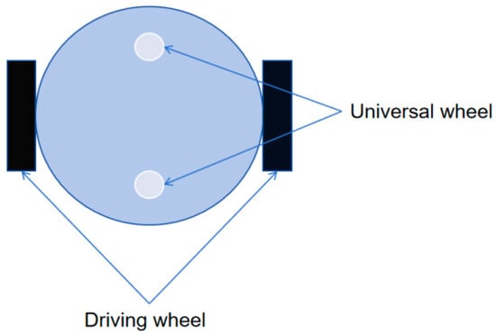
Figure 1.
Differential wheel chassis diagram.
The differential drive chassis design possesses relatively stable motion control characteristics, as it allows the robot to more flexibly adjust speed and direction during motion. This stable motion control is crucial for the performance and stability of SLAM algorithms. It can reduce errors and uncertainties during mapping and localization processes, thereby enhancing the navigation accuracy and reliability of the robot. Therefore, by selecting the differential drive chassis design, we can better meet the motion requirements of indoor service robots in complex environments and provide them with a stable and reliable motion control foundation.
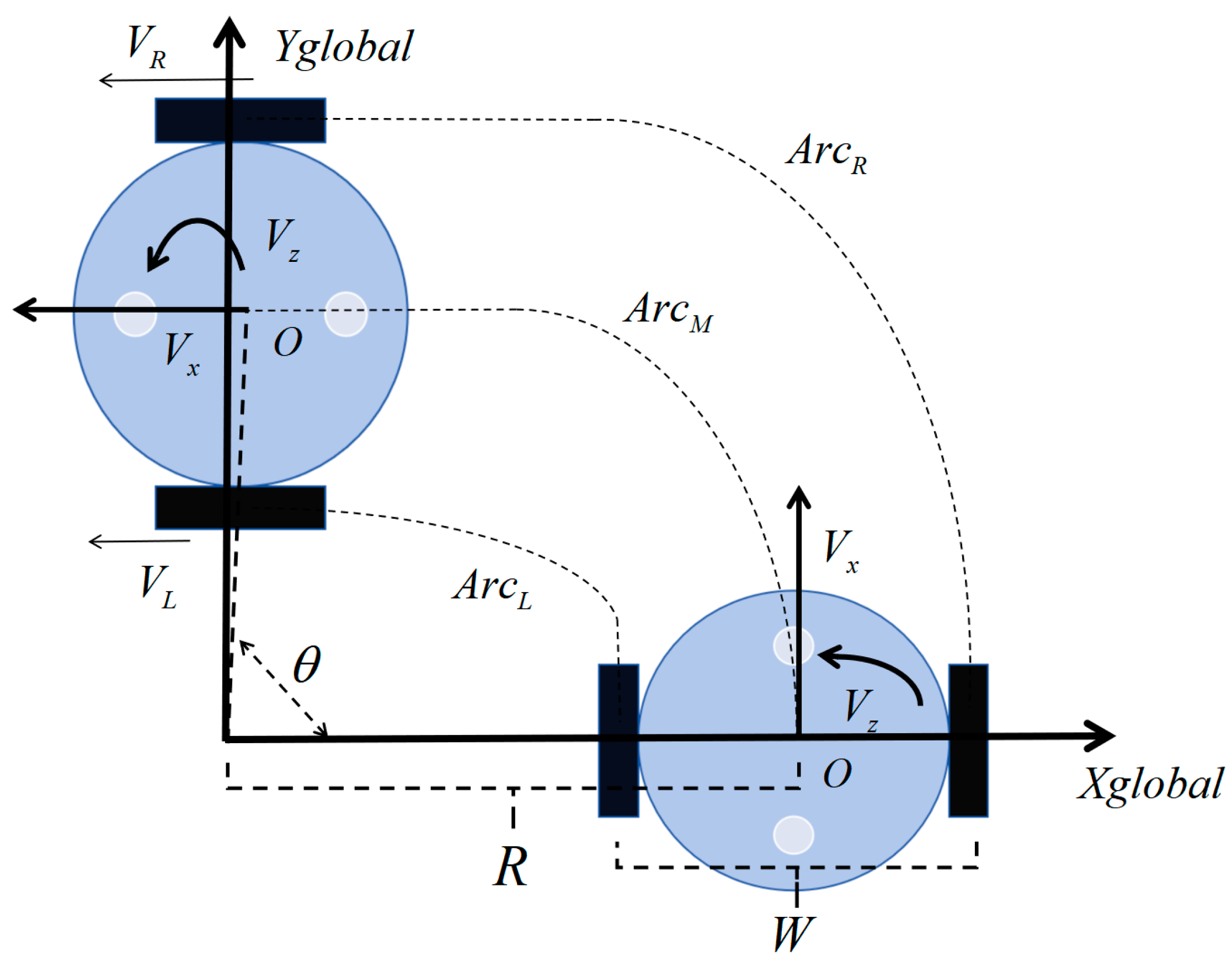
2.1.2. Kinematic Analysis
Below, we will conduct a kinematic analysis of the two-wheel differential drive chassis, as depicted in the schematic in Figure 2.

Figure 2.
Kinematic analysis structure of two-wheel differential chassis.
Next, the forward and inverse kinematics solution formula of the robot chassis is obtained:
where the distance from the center is point , , and represent the paths traveled by the left wheel, point , and the right wheel of the robot within a certain time t, measured in meters. is the turning radius generated by the robot simultaneously advancing and rotating, measured in meters. and are the speeds of the left and right wheels of the robot, positive for forward motion, measured in meters per second. W is the distance between the two drive wheels, measured in meters. is the angle that the robot rotates during a certain time t, measured in radians. The equation relating arc length to radius is given by dividing the arc length by the radius, resulting in radians:
Substitute , and into the equation:
Divide both sides of the equation by t, and then integrate with respect to time:
where is the target forward velocity of the robot at point , positive for forward motion, measured in meters per second. is the target rotational velocity of the robot around point , positive for counterclockwise rotation, measured in radians per second. Decomposing Equation (4) yields:
Formulas (5) and (6) are changed into the forward kinematics solution formula, and the current speed of the driving wheel and are known to find the real-time speed and of the current robot:
On the STM32F4 side, the process executed is the kinematic inverse solution. Through functions written in the C language, relevant parameters and are passed in, along with the robot’s velocity in the X and Y axes, to solve for the target velocities of the two motors. Through this process, precise control of the rotation speed of the drive wheels is achieved, allowing for accurate control of the robot’s motion.
2.2. Control System Design
The chassis control of the service robot stands as the nucleus of the entire robotic control system. Considering the computational capabilities, complexity of the encoder and motor control, and future optimization needs, our objective is to fully leverage the GPIO, timers, and serial port resources of the microcontroller chip for the development board. The STM32F407VET6 is a powerful and feature-rich microcontroller based on the ARM Cortex-M4 core, operating at a high frequency of up to 168 MHz. It comes equipped with a rich set of peripherals and functional modules, including multiple general-purpose timers and communication interfaces (such as USART, SPI, I2C, etc.). Additionally, the STM32F407VET6 incorporates a low-power design to ensure efficient power management while maintaining high performance, making it suitable for applications such as mobile robots that demand low power consumption. The STM32F407VET6 offers a high cost-effectiveness ratio relative to its performance and feature advantages, making it an excellent choice for widespread use in embedded systems, including robotics. Therefore, selecting the STM32F407VET6 as the main controller is well-suited to our project requirements.
The STM32F407VET6 microcontroller integrates a rich array of peripherals and communication interfaces, allowing direct connectivity with the MPU6050 sensor and TB6612 motor driver chip when integrated on a single development board. This integration simplifies hardware layout and interconnections, facilitating increased system integration and stability. The MPU6050 sensor integrates a three-axis gyroscope and three-axis accelerometer, enabling it to be used for robot attitude perception and motion control. The TB6612 motor driver chip supports the driving of DC motors and, when paired with Hall effect encoder motors, enables precise position and motion control. This combination enhances the robot’s motion stability and accuracy. To ensure efficient program execution, we leverage the portability, interrupt management, task operations, list queues, and software timers provided by the FreeRTOS operating system on the STM32 platform [11]. By designing and extending the control program within the FreeRTOS environment, we maximize system efficiency and leverage the capabilities of FreeRTOS for task management, interrupt handling, and overall system reliability.
Considering the practical requirements for low power consumption, cost-effectiveness, and a compact main control processor, along with the capability to smoothly run the ROS operating system, we have selected the Nvidia Jetson Nano B01 running on the Ubuntu 18.04 operating system environment. Compared to other high-end embedded computing platforms, the Jetson Nano B01 offers high-performance computing capabilities at a relatively lower price point, making it highly cost-effective and suitable for robot applications where cost efficiency is important.
The Nvidia Jetson Nano B01 provides a balance of performance and affordability, making it an ideal choice for robotics applications that require computational power within budget constraints. Its compatibility with Ubuntu and ability to support ROS enable seamless integration into robotics projects, facilitating tasks such as perception, planning, and control. Overall, the Jetson Nano B01 aligns well with the requirements of robotics applications that prioritize cost efficiency without compromising on performance. Given the memory requirements of the Jetson Nano B01’s central processing unit (CPU) and graphics processing unit (GPU) need to remain within reasonable bounds, while ensuring the service robot achieves low inference time and superior recognition accuracy in object detection tasks, we decide to employ the YOLOv3 algorithm under the Darknet framework. To maximize hardware resource utilization, we choose a lower computational power RGB camera for the recognition module. Such a configuration not only meets the algorithmic demands but also efficiently utilizes hardware resources, thereby enhancing the overall performance and efficiency of the system.
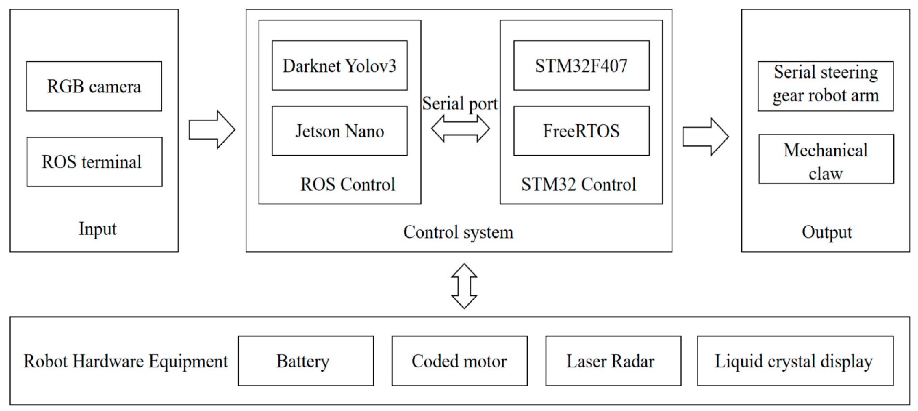
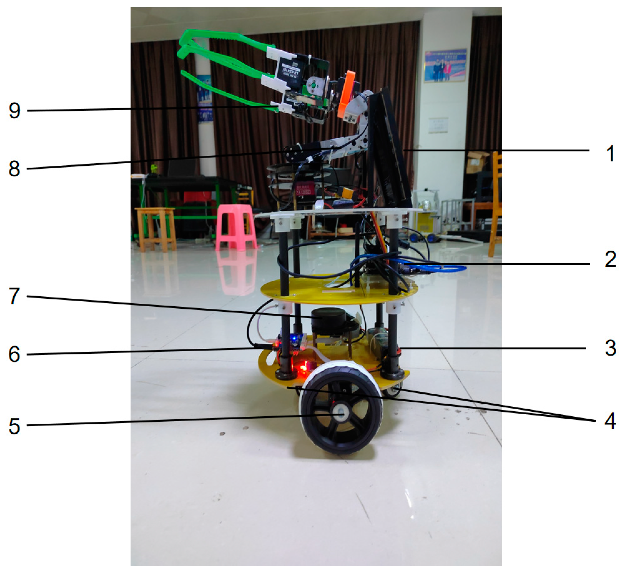
The overall system architecture, as depicted in Figure 3, comprises two main components: the ROS side and the STM32 side, interconnected via serial communication. These two ends collaboratively facilitate robot motion control. Hardware devices of the robot exchange information with the control system, enabling the execution of corresponding functions. The robot can obtain input information from the camera or ROS terminal, process it through the control system, and execute the corresponding functions via the output mechanism. A conceptual prototype of the robot, as illustrated in Figure 4, includes the RPLIDAR A1 and STM32F407 at the bottom layer, responsible for low-level hardware control and sensor data acquisition. Positioned on the second layer, the Jetson Nano undertakes data processing and high-level control. The mechanical arm, equipped with a camera, resides at the top layer, responsible for executing object detection tasks.
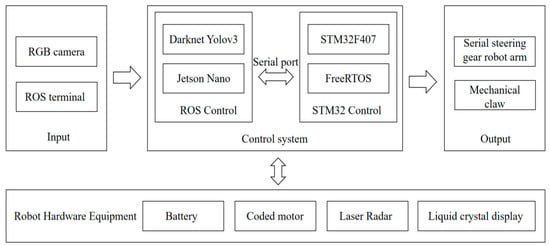
Figure 3.
Block diagram of robot system structure.

Figure 4.
Structure diagram of robot prototype. 1—Liquid crystal display, 2—Nvidia Jetson Nano B01, 3—Battery, 4—Universal wheel, 5—Driving wheel, 6—STM32F407 Core Board, 7—Laser Radar, 8—Serial steering gear robot arm, 9—RGB camera.
2.3. Robot Vision Part Design
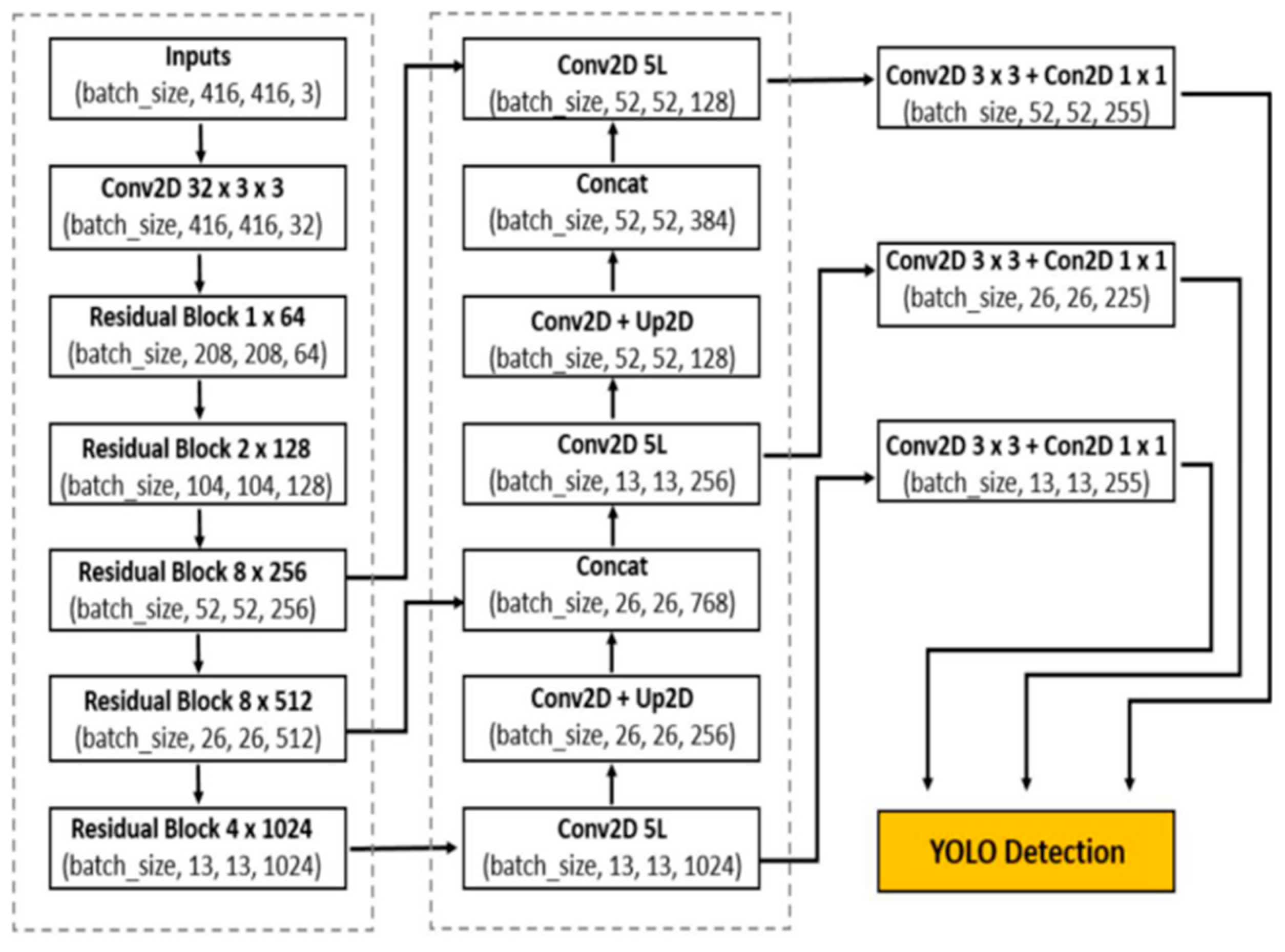
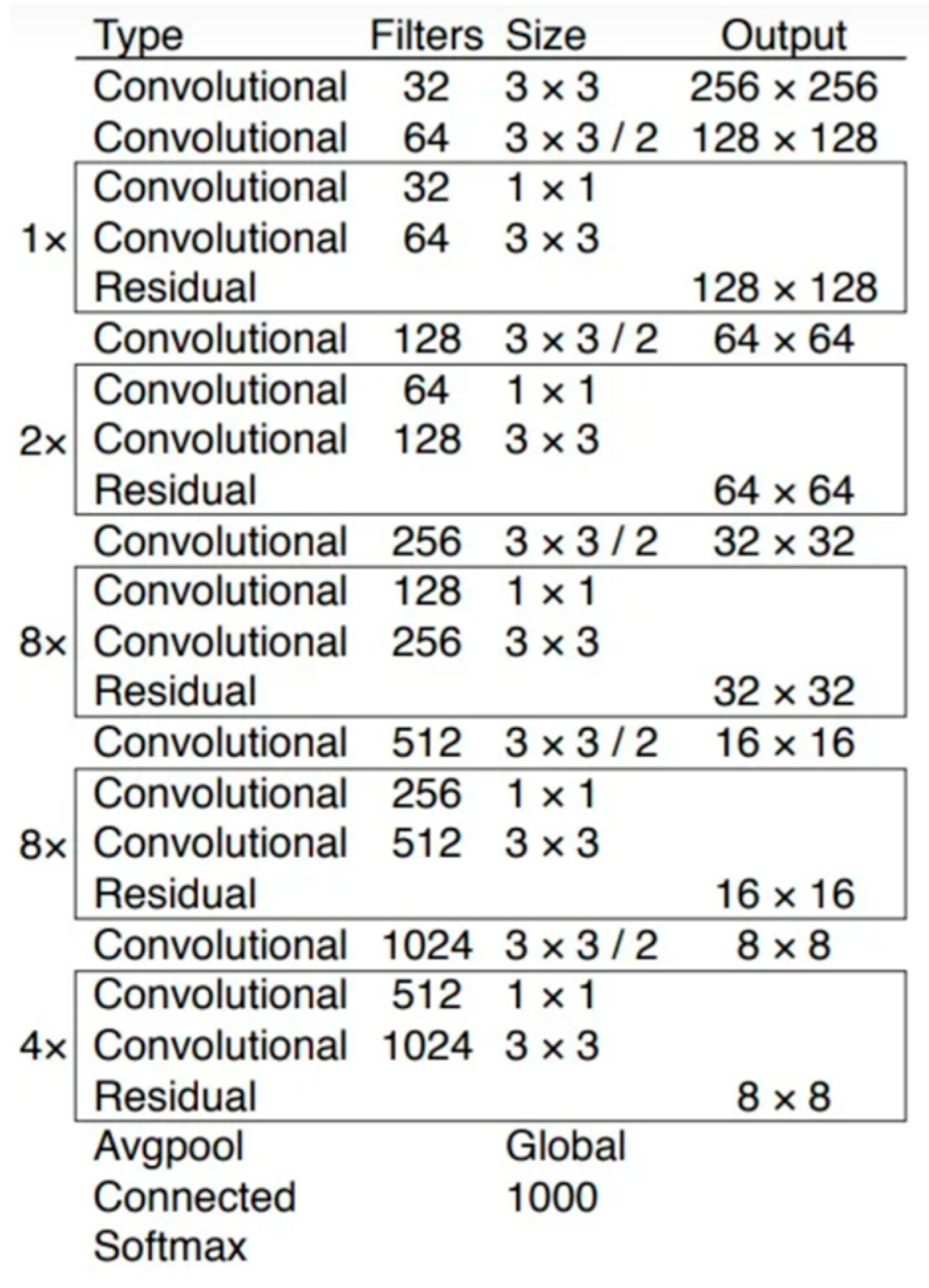
Presently, deep learning methods have emerged as the focal point of research in the field of object detection, particularly those based on convolutional neural networks (CNNs). CNNs excel in accurately processing visual data without the need for separate feature extraction processes [12]. In this study, we employed the YOLOv3 algorithm, depicted in Figure 5, which represents an improvement over its predecessors, YOLOv1 and YOLOv2 [13]. Built upon the Darknet deep learning framework, as illustrated in Figure 6, this algorithm boasts exceptional hierarchical feature extraction, learning capabilities, and efficient processing of large-scale data on specific hardware environments. This enables it to better meet the requirements of object detection algorithm systems for recognition accuracy and real-time performance.
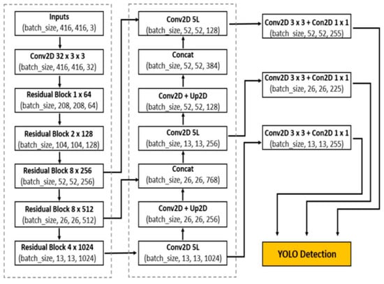
Figure 5.
YOLOv3 frame diagram.
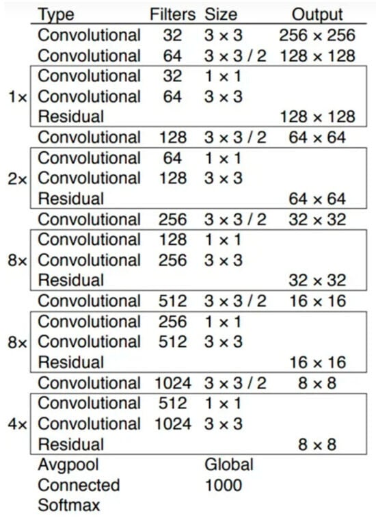
Figure 6.
Darknet frame diagram.
By collecting image data from the camera and preprocessing them before inputting them into the network, including data augmentation and input adjustments [14], the algorithm ensures optimal performance. Through the forward propagation of neural networks, the Darknet-53 backbone network is utilized to extract image features, generating object detection results via multiple layers of convolution and detection layers.
The neural network architecture primarily consists of a backbone network and three detection scales (13 × 13, 26 × 26, 52 × 52). Its backbone network is built upon Darknet53, replacing DarkNet-19 to become the new feature extractor for YOLOv3 [15]. YOLOv3 utilizes Darknet-53 to extract features of target objects, constructing three different scale feature maps [16], with their respective parameters outlined in Table 1. Compared to DarkNet-19, ResNet-101, and ResNet-152 networks, DarkNet-53 exhibits significant advantages in terms of Top-1 accuracy, Top-5 accuracy, and floating-point operations per second [17]. The CBL module represents the convolutional structure, followed by BN normalization to reduce overfitting, and Leaky RELU is chosen as the activation function.

Table 1.
Comparison table of DarkNet-53 network parameters with those of DarkNet-19, ResNet-101, and ResNet-152 networks.
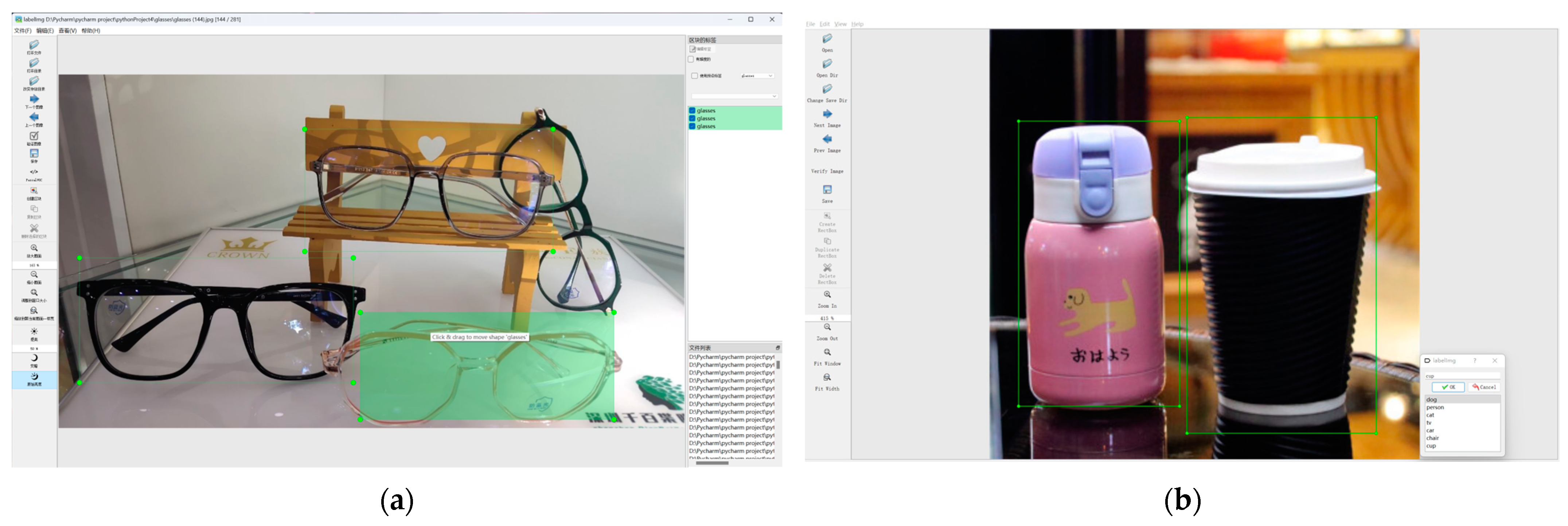
The experiment utilized the VOC dataset, comprising five categories: chair, pen, glasses, USB drive, and cup, totaling 1488 images. The dataset annotation process is illustrated in Figure 7. The dataset was divided into 70% training set, 20% validation set, and 10% test set. By adjusting network parameters, the objective was to train the object detection model to adapt to the characteristics of the VOC dataset and enhance performance. Target features and positional information were learned on the training set, and network weights were iteratively optimized through multiple epochs to achieve more accurate detection results. The GeForce RTX 4080 GPU on Ubuntu 18.04 was chosen to train the YOLOv3 network to fully leverage hardware performance. Training parameters were repeatedly adjusted to obtain a series of experimental results, and a model with good performance was selected through comparison. When evaluating model performance, attention was paid to precision, recall, F1 score, and average precision (AP), with mAP calculated as a comprehensive metric.
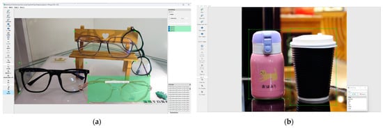
Figure 7.
Figure (a) shows the process of labeling glasses using labelImg, and Figure (b) shows the process of labeling cups using labelImg.
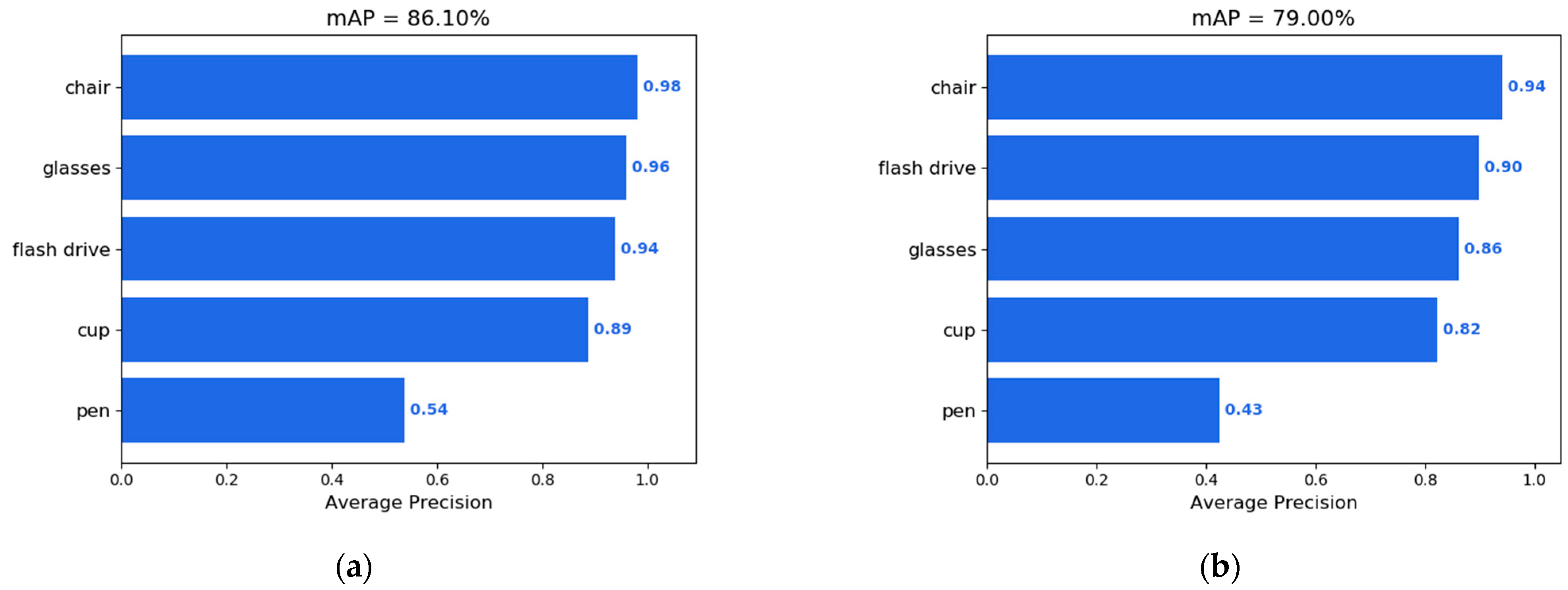
In terms of optimization algorithm selection, we compared the use of Adam and SGD, two different optimization algorithms. The detection results of each algorithm on the dataset are presented in Table 2. By examining the performance indicators in the table and contrasting different experimental results, particularly those depicted in Figure 8, specifically Figure 8a,b, we have drawn several important conclusions:
Table 2.
Each algorithm detects the result on the data set.
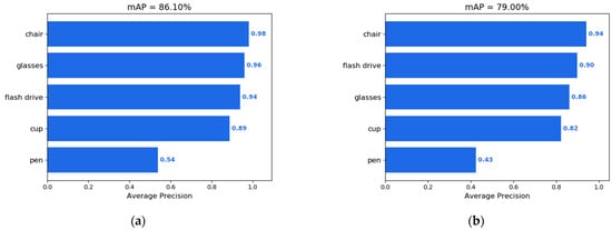
Figure 8.
Figure (a) is the actual test interface, and Figure (b) is the test result of the office environment. Figure (a) shows the output result of Adam mAP, and Figure (b) shows the output result of SGD mAP.
- The Adam optimization algorithm exhibits a higher mAP value compared to SGD, indicating that Adam is more suitable for object detection tasks based on comprehensive evaluation.
- We also considered precision, recall, and F1 score to comprehensively assess model performance, assisting in balancing accuracy and comprehensiveness.
- After thorough parameter tuning and comparative experiments, it was confirmed that the Adam optimization algorithm performs better in object detection, displaying significant advantages across various metrics.
- The comprehensive experimental results provide strong support for selecting outstanding object detection models, highlighting the importance of optimization algorithms in performance and offering valuable guidance for practical applications.
Upon obtaining the available weight files, we successfully ported them to the YOLOv3 algorithm package on the Jetson Nano B01. Environmental data were captured in real time using an RGB camera for perception. The main controller processed this data and evaluated the recognition results. Ultimately, the results were fed back on the display screen and printed in the ROS terminal. This system architecture allows us to effectively apply image processing tasks to service robots while ensuring processing efficiency and accuracy.
3. Experimental Design and Results
3.1. Experimental Design
Firstly, we will conduct simulation experiments using three different SLAM algorithms to map and navigate in a simulated environment. This step aims to evaluate the performance of different algorithms under ideal conditions and compare their differences. Subsequently, we will replicate the map environment of the simulation experiments in real scenes and conduct experiments in real-world scenarios to verify the feasibility and applicability of the simulation results in actual environments. This will help determine the accuracy of the simulation results in real environments and whether adjustments or improvements to our solution are necessary. Next, we will conduct experiments in more complex real-world scenarios to assess the robustness and resilience of the solution in different environmental conditions. By experimenting in different scenes and conditions, we will evaluate the performance of algorithms and technologies, optimize parameters to improve performance, and further enhance the effectiveness of the solution. The purpose of this series of experimental designs is to comprehensively validate the reliability and practicality of the robot solution, providing sufficient support and assurance for its deployment in real-world applications.
3.2. SLAM Simulation Experiment
A SLAM system that uses only a laser rangefinder or integrates other sensors with a laser rangefinder is referred to as a laser SLAM system [18]. In our system, the sensor module selection includes a laser rangefinder and an inertial measurement unit (IMU) for collecting environmental information. Through the processing of mapping algorithms, a two-dimensional map is ultimately generated. Classical laser SLAM algorithms include the Gmapping algorithm, Cartographer algorithm, and Hector-SLAM.
3.2.1. Virtual Simulation Environment
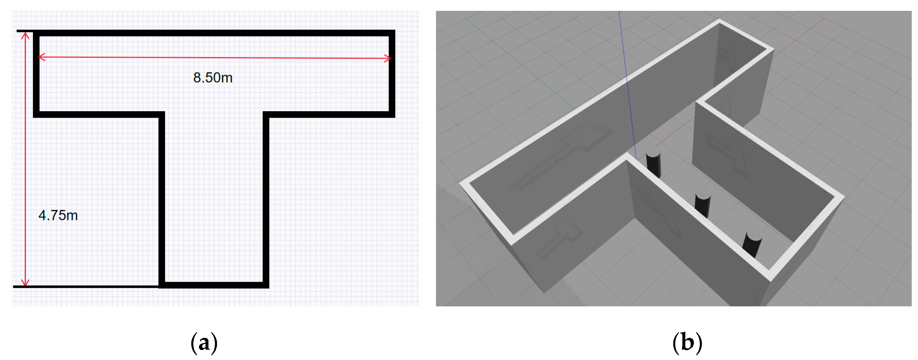
In order to verify the above algorithms, we conducted simulation experiments on the Gazebo platform and built the simulation environment as shown in Figure 9. We designed the virtual environment to ensure that it has real physical characteristics, so that the simulation results are highly referential and can effectively reflect the situation in the real environment.
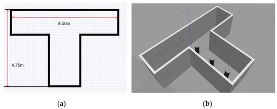
Figure 9.
Set up the virtual simulation environment in Gazebo. Figure (a) is a plane diagram, and Figure (b) is a three-dimensional diagram.
Using a laser rangefinder as the sensor, we simulated the GMapping, Hector-SLAM, and Cartographer algorithms. We established a simulation environment in the Gazebo platform that corresponds to the experimental site and tested these three different SLAM algorithms. We compared the quality of the final effect maps. During the mapping process, the known environment layout is represented in light gray, while the data collected by the laser rangefinder are presented with red markers.
3.2.2. GMapping
To estimate the robot’s pose, we utilize the Rao-Blackwellized particle filter (RBPF) [19]. The core idea of particle filtering is to represent probabilities using a particle set, and the most commonly used algorithm in particle filtering is the Importance Resampling algorithm. This algorithm iteratively predicts the robot’s pose, and it consists of the following five steps:
- Sampling: According to the motion model, sampling is conducted on the preceding generation of particles, denoted as particle ‘’, yielding the emergence of novel particles termed ‘’. These particles are utilized to forecast the posture of the robot by amalgamating the most recent motion data.
- Calculated weight: Within the framework of particle filtering, the utilization of sensor measurements and motion models allows for the computation of the weight associated with each new particle. These weights are then allocated to individual particles, thus providing a more precise representation of the robot’s actual position within its environment.
- Resampling: Particles endowed with higher weights are preserved, whereas those with lower weights are eliminated. This process aids in concentrating the distribution of particles, thereby enhancing the efficiency of the filtering algorithm.
- Map estimation: By employing the Rao-Blackwellization technique, the degree of congruence between observation data and the map can be assessed. This facilitates the inference of the conditional probability of observation data under a given map, thereby enabling the updating of particle weights.
- Based on RBPF, selective resampling and proposal distribution are improved: These enhancements contribute to the enhancement of the algorithm’s performance in practical applications, enabling the robot to construct and update environmental maps more reliably, thus improving the performance and robustness of mapping algorithms.
- Selective resampling: As particles are solely responsible for representing the robot’s pose, it is feasible to estimate the map by conditioning on the updated particle set. This ensures that the particle set effectively reflects both the robot’s state and map information.
- Improved proposal distribution: To accurately simulate the state distribution, it is imperative to discard particles with lower weights and replicate particles with higher weights, thereby concentrating the particle set closer to the true state.
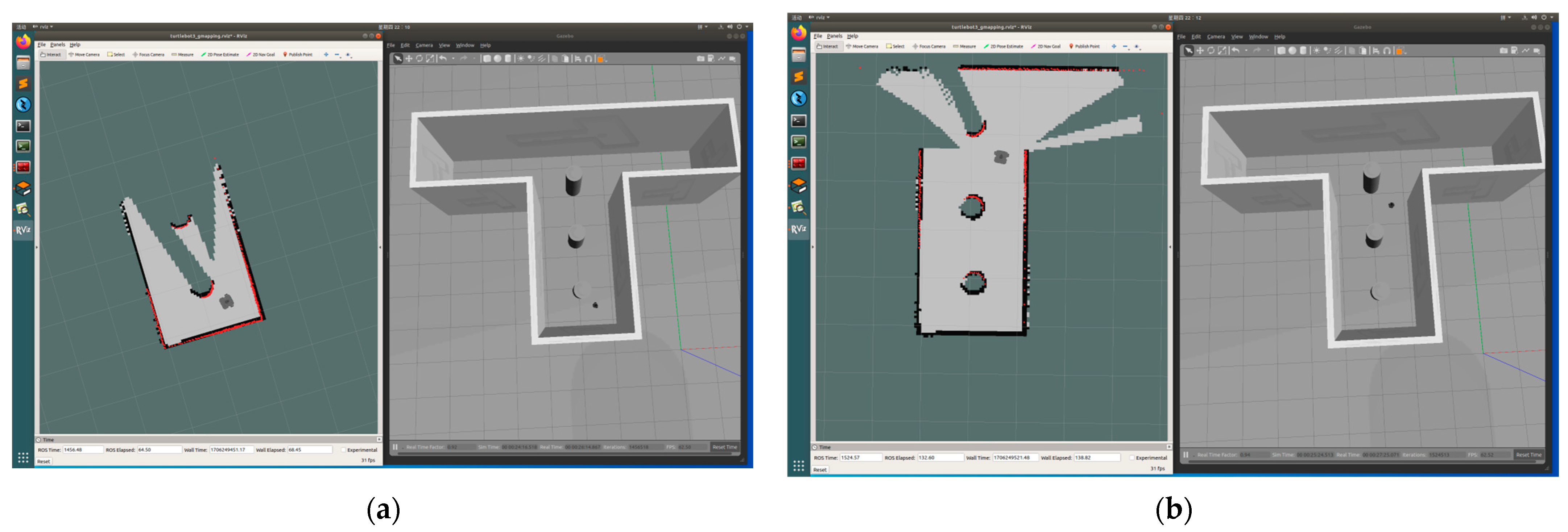
Figure 10 illustrates the simulated results of the GMapping algorithm. During the mapping process, laser sensor data are utilized to match the poses of particles and the map. By aligning the poses of particles and the map, the weights of particles are updated. Subsequently, resampling is conducted, and the grid map is updated based on the poses of particles with higher weights. This process effectively utilizes laser sensor data to continuously optimize the grid map, reflecting the true state of the environment.
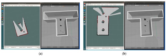
Figure 10.
Set mapping process of GMapping. Figure (a) is the initial state of the experiment, and Figure (b) is the state of the experiment process.
3.2.3. Hector-SLAM
Hector-SLAM stands as a renowned open-source 2D SLAM system, dedicated to laser data map construction and distinctive localization methods. Initially, acquiring laser data as the first frame, by time t, the algorithm matches laser scan data with the map from time t − 1, thereby determining the robot’s pose. This process aims to maximize the utilization of laser scan points to optimize the robot’s positioning within the environment [20]. The key features of Hector-SLAM include robust real-time performance, support for single-laser radar, and highly optimized occupancy grid maps. Its algorithmic steps encompass initialization, scan matching, feature extraction, occupancy grid map updating, tracking, loop closure detection, and output. This algorithm is suitable for scenarios demanding rapid localization and map construction, such as mobile robots and autonomous vehicles. Due to its simple yet efficient design, Hector-SLAM has garnered extensive applications in mobile robotics and embedded systems.
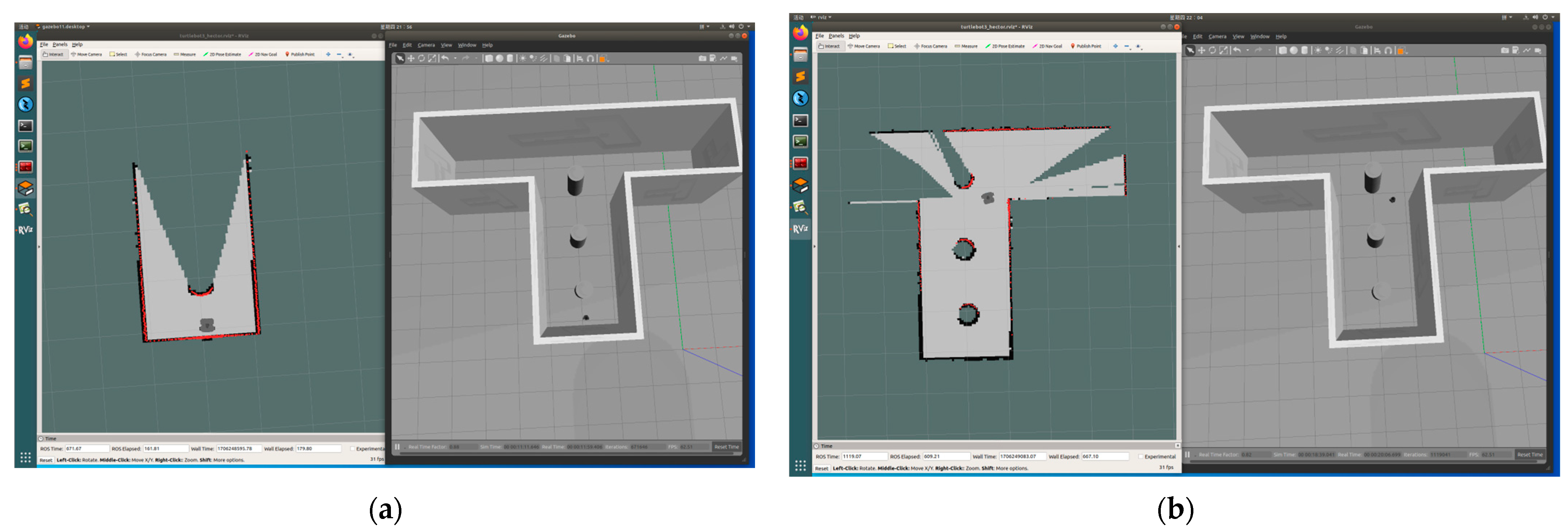
Figure 11 illustrates the results of simulated simulation utilizing the Hector-SLAM algorithm. By matching the current frame with the previous frame’s laser radar data, the algorithm estimates the robot’s motion. Simultaneously, certain features are extracted from the laser radar data, such as edges and corners, to aid subsequent localization and map construction. Based on the matching results and feature extraction, the Hector-SLAM algorithm updates the occupancy grid map, accurately reflecting the robot’s position in the environment and the distribution of obstacles. This process contributes to the establishment of precise and comprehensive environmental maps.
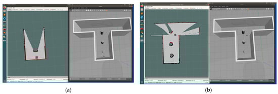
Figure 11.
Set mapping process of Hector-SLAM. Figure (a) is the initial state of the experiment, and Figure (b) is the state of the experiment process.
3.2.4. Cartographer
The Cartographer algorithm, a graph-based optimization approach, serves as Google’s solution for SLAM. Its open-source code comprises two main components: Cartographer and Cartographer_ROS. Employing graph-based mapping techniques, the Cartographer algorithm enables real-time acquisition of relatively high-precision 2D maps, suitable for large-scale mapping [21]. Its functionalities encompass processing data from sensors such as laser radar, IMU, and odometry to construct maps. Subsequently, Cartographer_ROS utilizes the ROS communication mechanism to acquire sensor data and convert it into Cartographer’s format for processing [22]. Furthermore, Cartographer_ROS is responsible for displaying or storing the processing results from Cartographer. This integrated process facilitates the convenient use of Cartographer for real-time SLAM applications within ROS. The authors of this software have extensively described impressive real-time results achieved by the software in addressing 2D SLAM problems [23].
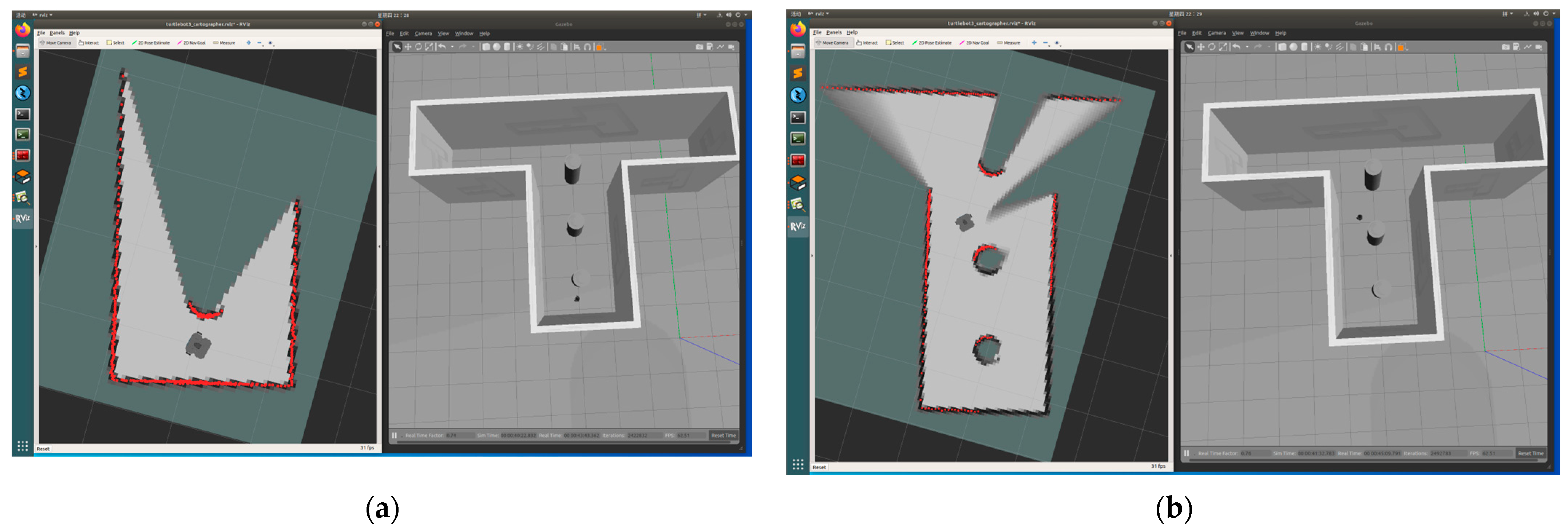
Figure 12 illustrates the results of simulated simulation using the Cartographer algorithm. In the initial stage, initial localization is performed to estimate the robot’s initial position. Subsequently, motion estimation is conducted by scan-matching the laser radar data from the current frame with the data from the previous frame. Throughout the mapping process, loop-closure detection is performed to enhance the consistency and accuracy of the map when the robot revisits previously accessed locations. The area scanned by the laser radar transitions from light gray to white as the entire map is completed. Finally, optimized robot trajectories and constructed 3D maps are outputted. This series of steps effectively demonstrates the efficiency and accuracy of the Cartographer algorithm in the mapping process.
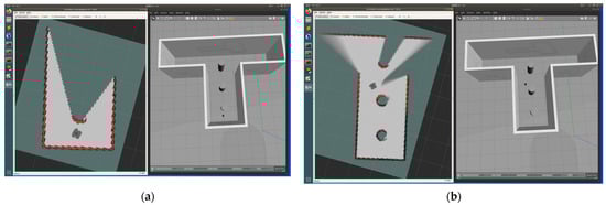
Figure 12.
Set mapping process of Cartographer. Figure (a) is the initial state of the experiment, and Figure (b) is the state of the experiment process.
3.2.5. Results of SLAM Simulation Mapping Experiment
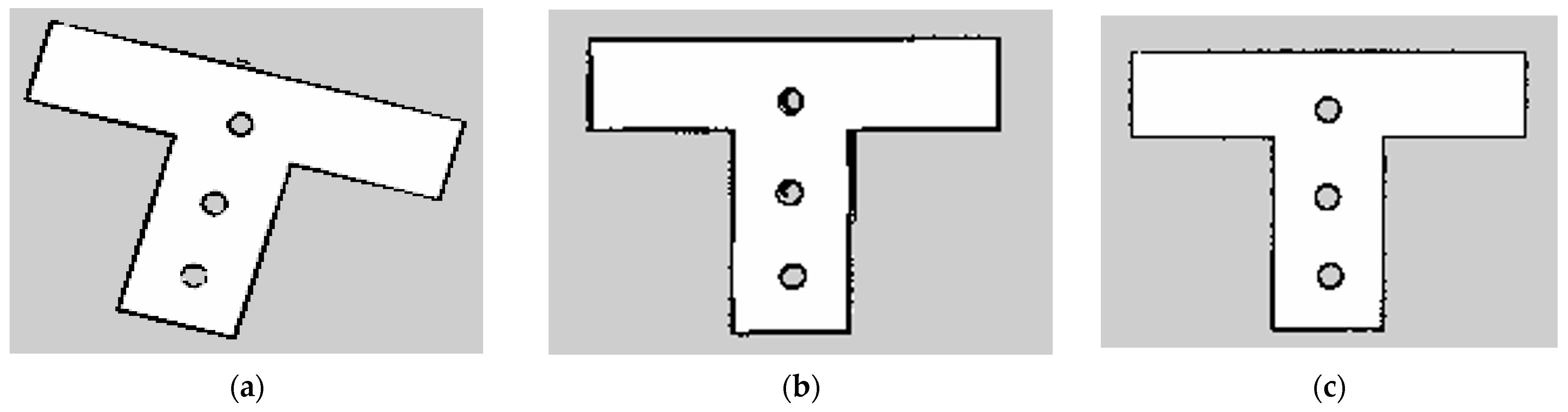
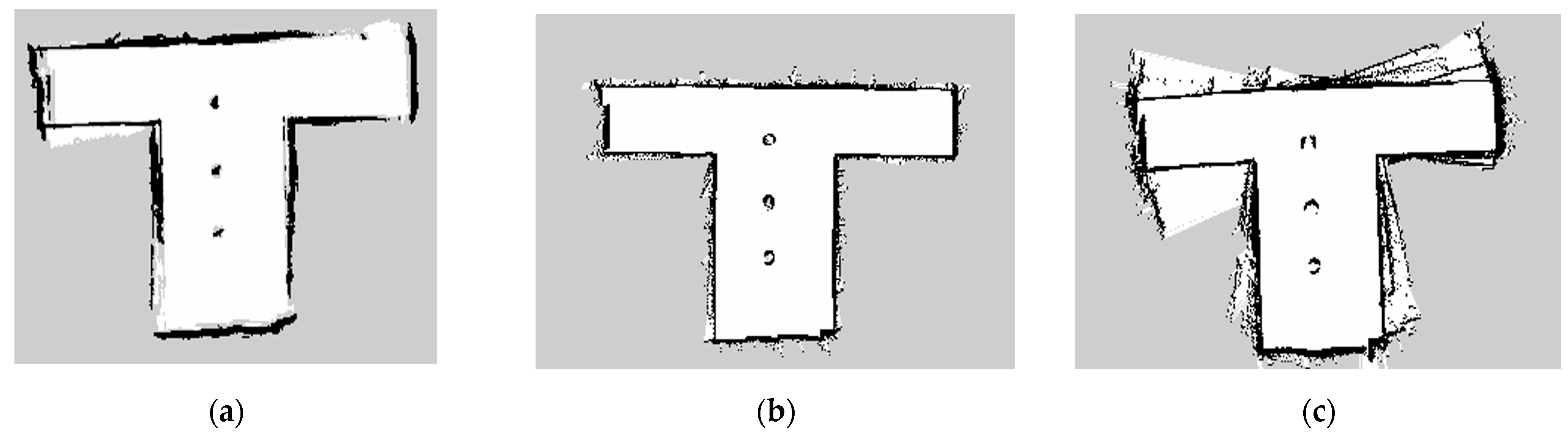
In terms of computational time, both the Hector-SLAM and GMapping algorithms exhibit shorter processing times compared to Cartographer. Regarding mapping effectiveness, the maps generated by Hector-SLAM and GMapping algorithms appear more organized compared to Cartographer’s output. Conversely, Cartographer’s maps exhibit numerous jagged edges and irregularities along the walls. Furthermore, upon further comparison between the Hector-SLAM and GMapping algorithms, the maps produced by Hector-SLAM algorithm exhibit a more aesthetically pleasing appearance and closely resemble real-world scenes. These observations underscore the importance of considering not only computational efficiency but also factors such as map quality and appearance when selecting SLAM algorithms. The mapping results of the three algorithms are depicted in Figure 13.
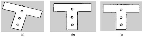
Figure 13.
Output result of the simulation experiment. Figure (a) shows the output of Cartographer, Figure (b) shows the output of GMapping, and Figure (c) shows the output of Hector-SLAM.
3.3. Path Planning and Navigation Simulation Experiments
3.3.1. Global Path Planning Using Dijkstra’s Pathfinding Algorithm
The fundamental principle of the Dijkstra algorithm is simple and intuitive, making it applicable to various scenarios. The Dijkstra algorithm, a shortest-path routing method, is used to compute the minimum cost of moving from one node to all other nodes. Its main feature is the expansion from the initial node outward layer by layer until reaching the target node [24]. The algorithm expands outward layer by layer, creating two lists: the Open list and the Closed list. The Open list stores points on the path to be determined, while the Closed list stores points on the path that have been determined. Each point records its parent node and the distance to the initial point. The algorithm starts from the initial point, selects the node with the minimum distance in the Open list as the center point, moves it into the Closed list, and adds its unvisited neighboring nodes to the Open list. This process is repeated until the expansion reaches the target node. Finally, based on the recorded parent nodes, the shortest path is extracted by propagating information in reverse.
3.3.2. Local Path Planning teb_local_planner
The teb_local_planner stands out as a premier navigation algorithm within the ROS framework, focusing on achieving local path planning through the optimization of time and space. At its core lies the technique of trajectory rollout and elastic band (TEB), which employs the Timed Elastic Band algorithm—an enhanced approach akin to a rubber band method, aimed at path planning for robots by considering time–space optimization [25]. TEB has the capability to consider dynamic obstacles when computing velocity commands [26], with the objective of striking a balance between trajectory smoothness, robot dynamics, and obstacle-avoidance performance. TEB allows robots to plan smooth trajectories in local environments while also accounting for the robot’s dynamic characteristics and obstacle-avoidance requirements. The advantage of this approach lies in providing a path-planning strategy adaptable to changes in dynamic environments, as illustrated in Equation (9).
and represent the left and right wheel speeds of the robot, with forward as positive, in units of meters per second. denotes the distance between the two drive wheels, measured in meters. Relative to the Dynamic Window Approach (DWA) algorithm, the Timed Elastic Band (TEB) algorithm offers significant advantages in several aspects including path optimization, dynamic obstacle handling, path trajectory smoothness, consideration of time factors, and comprehensive integration of robot dynamics constraints. According to experimental conclusions by Jiaying Guo, the TEB algorithm demonstrates superior performance in local path planning, successfully navigating through obstacles to reach specified target points while avoiding collisions or getting stuck, outperforming the DWA algorithm overall [27]. Therefore, the TEB algorithm is better suited for applications such as indoor service robots that require flexible and real-time path planning. It significantly enhances robot navigation performance and path-planning quality, providing reliable support for safe robot movement in complex environments.
3.3.3. Path Planning Simulation Experiment
After obtaining the corresponding mapping map, global and local path planning is conducted using the previously described path-planning algorithms. Within the ROS framework, the rviz software 1.14.20 package is utilized for path planning and navigation simulation. The constructed map, as shown in the left image, depicts black dots representing obstacles, green regions indicating the safe distance between the robot and obstacles, and red arrows indicating the target point and direction of the robot. The entire map enclosed by the blue box represents the global map, while the square blue box surrounding the robot represents the local map. Figure 14 displays the results of path planning and navigation, presented as green lines. The starting position of the robot is slightly below the obstacles. From the simulation results, it can be observed that the generated path successfully avoids the obstacles, representing a relatively suitable path.
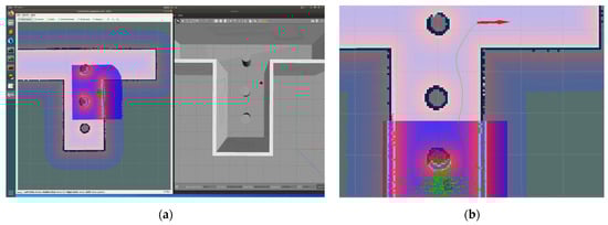
Figure 14.
Process of path planning and navigation. Figure (a) is the schematic diagram of the path-planning simulation experiment, and Figure (b) is the schematic diagram of the path-planning experiment route amplification.
3.4. SLAM Live Field Experiment
We will replicate the simulation environment map in the actual field to test the three SLAM algorithms and select the most effective one based on the real-world scenario for subsequent path-planning experiments. The actual experimental site is depicted in Figure 15:
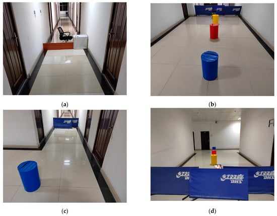
Figure 15.
Test site. Figure (a) is the right side of the T-shaped field of the experiment site, Figure (b) is the interchange of the T-shaped field of the experiment site, Figure (c) is the left side of the T-shaped field of the experiment site, and Figure (d) is the overall schematic diagram of the experiment site.
3.4.1. SLAM Actual Site Construction Process
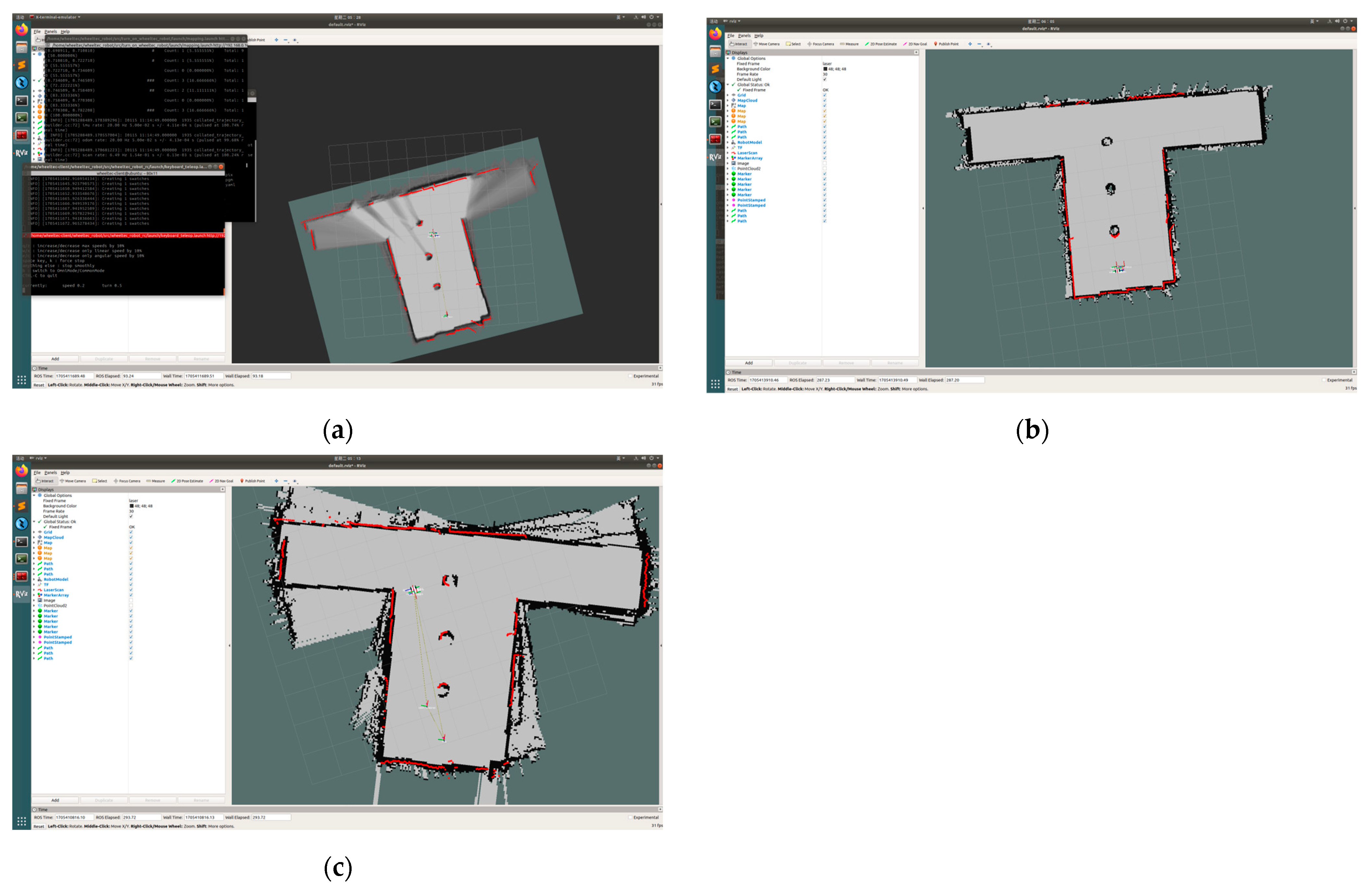
During the experimental process, we consistently started the robot from the same initial point for SLAM mapping experiments. We aimed to maintain a steady speed for the robot as it approached various adjacent boundaries, ensuring optimal mapping output quality. This approach helped ensure that the mapping results were as accurate and effective as possible. The construction process of the three algorithms is shown in Figure 16.
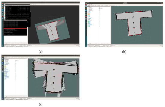
Figure 16.
The experimental process of the site experiment in the simulated environment. Three algorithmic mapping processes. Figure (a) shows the construction process of Cartographer, Figure (b) shows the construction process of GMapping, and Figure (c) shows the construction process of Hector-SLAM.
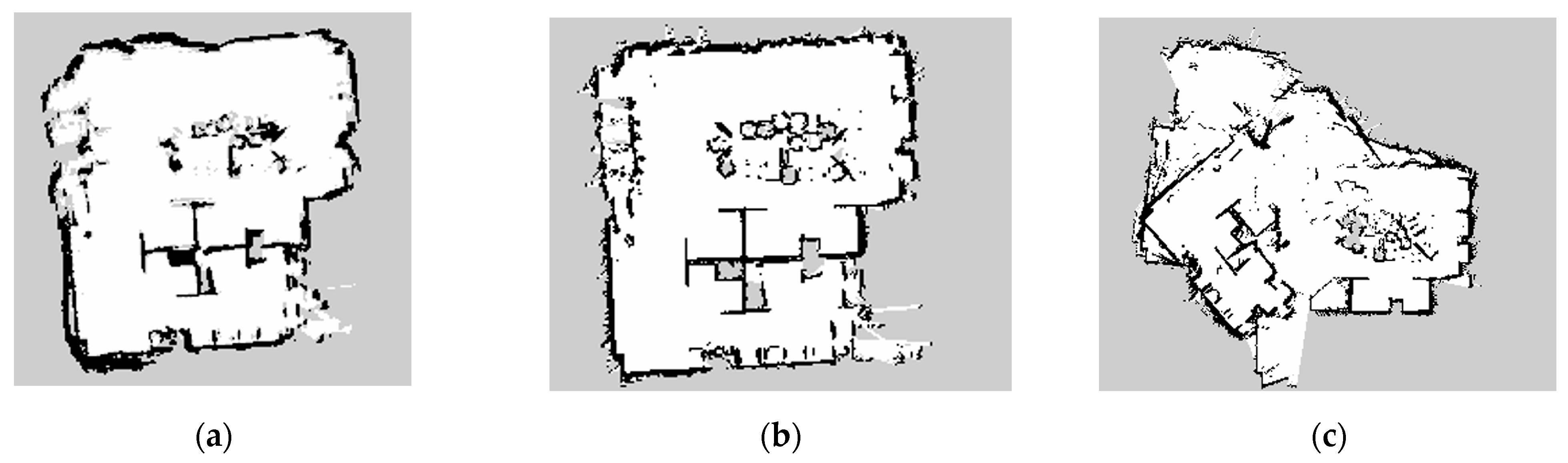
3.4.2. SLAM Actual Site Construction Results
The results of the three algorithms are shown in Figure 17. Compared with the simulation results, only the Gmapping algorithm is satisfactory.
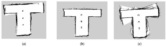
Figure 17.
Output result of experiment site that replicates the simulation environment. Figure (a) shows the output of Cartographer, Figure (b) shows the output of GMapping, and Figure (c) shows the output of Hector-SLAM.
3.4.3. Practical Path Planning and Navigation Experiments
During the path-planning stage, we utilize the Dijkstra algorithm as the global path-planning algorithm, while the teb_local_planner algorithm is employed for local path planning. Through this combination, we can achieve the overall path planning and motion process of the robot.
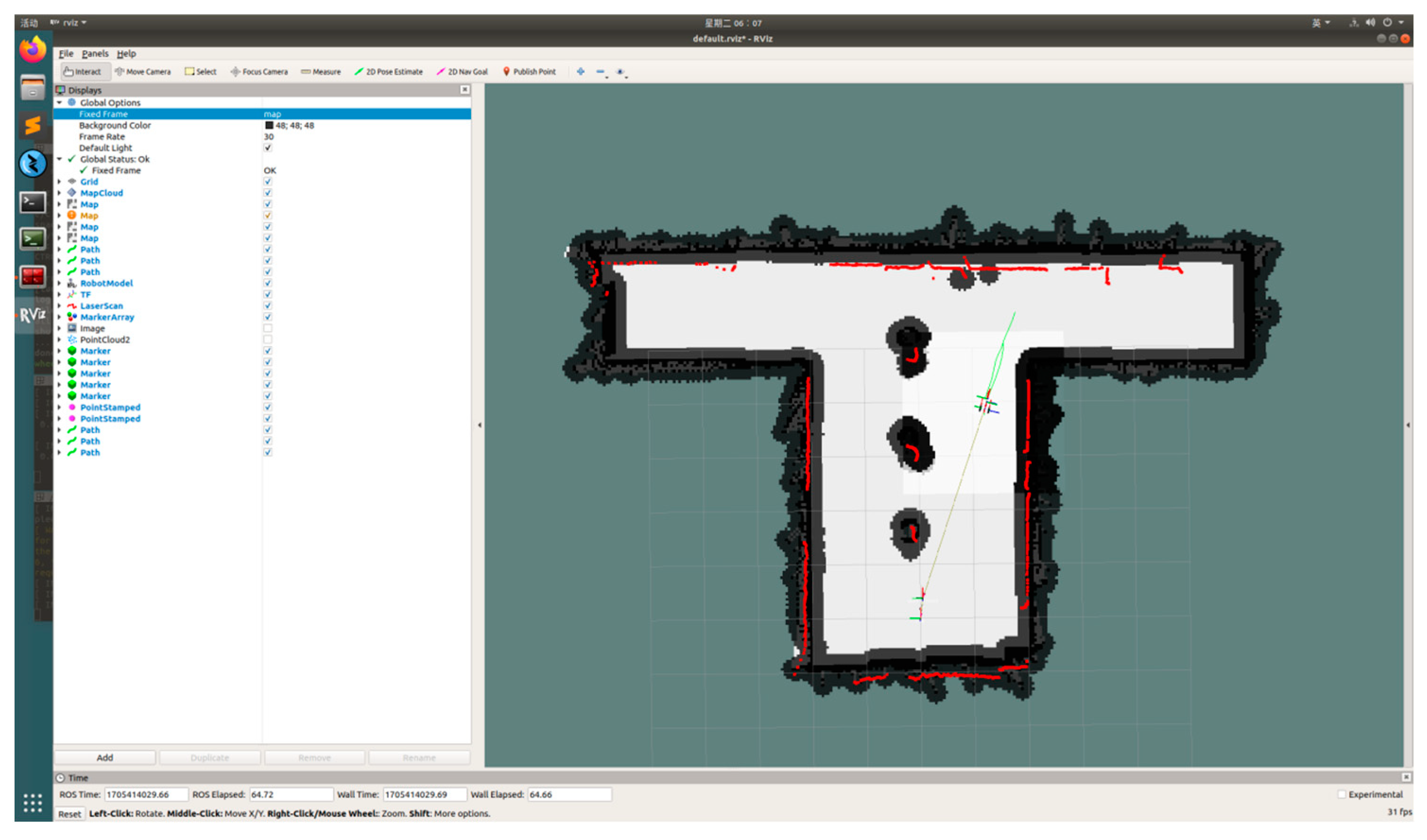
Figure 18 illustrates the process of path planning and navigation, with the robot heading towards the set endpoint. The planned path is represented by green lines, with the black area surrounding the map being the Global map, and the white box around the robot representing the Local map. Thus, we can verify the feasibility and effectiveness of the selected path-planning algorithm in the actual field. This experimental result will help confirm the selection of the optimal SLAM algorithm and demonstrate the effectiveness of path planning in real-world applications.
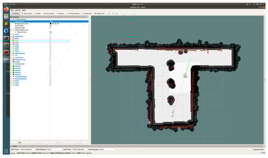
Figure 18.
Process of path planning and navigation.
3.4.4. Real Scene Target Detection
During the robot’s movement towards the target point, it will lift its robotic arm to ensure that the camera accurately aligns with the small objects that need to be identified. This step aims to ensure that the camera can capture clear images. Once the robot reaches the target point and lifts the robotic arm, the RGB camera starts capturing images and transmits them to the target recognition algorithm. This algorithm utilizes computer vision techniques to process the images and identify objects within them. The process of object detection in the experimental field is depicted in Figure 19. Before starting the experiment, we placed common small items that might be found in an office environment at the robot’s destination. We then waited for the robot to reach the designated target point, at which point the robot began the process of identifying the items. During the identification process, according to the experimental setup, the recognition algorithm categorizes objects in the images and locates the target objects. As described, the red box represents the identified office chair with confidence scores of 0.91 and 0.51; the yellow box represents the identified water cup with confidence scores of 0.55, 0.62, and 0.86; the blue box represents the identified pen with a confidence score of 0.59; the green box represents the identified USB drive with a confidence score of 0.71; and the purple box represents the identified glasses with a confidence score of 0.95.
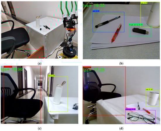
Figure 19.
Picture of the robot performing target detection in the experimental site. Figure (a) shows that the robot is in the recognition state. Figure (b) shows that it has recognized pens, USB disks and water cups. Figure (c) shows that it has recognized office chairs and water cups. Figure (d) shows that it has recognized office chairs, water cups and glasses.
3.5. Office Real Site Experiment
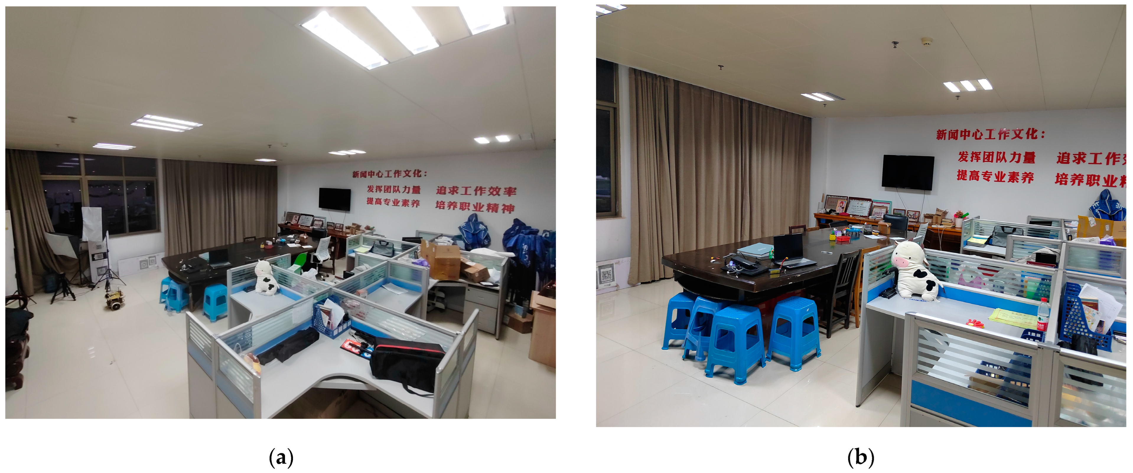
We will replace the experimental field with an office scene and conduct SLAM experiments in a real office environment. The actual experimental site is depicted in Figure 20.

Figure 20.
Schematic diagram of the actual office site Figure (a) is a panoramic view of the office, and Figure (b) is a view of the main working areas of the office.
3.5.1. SLAM Office Site Construction Process
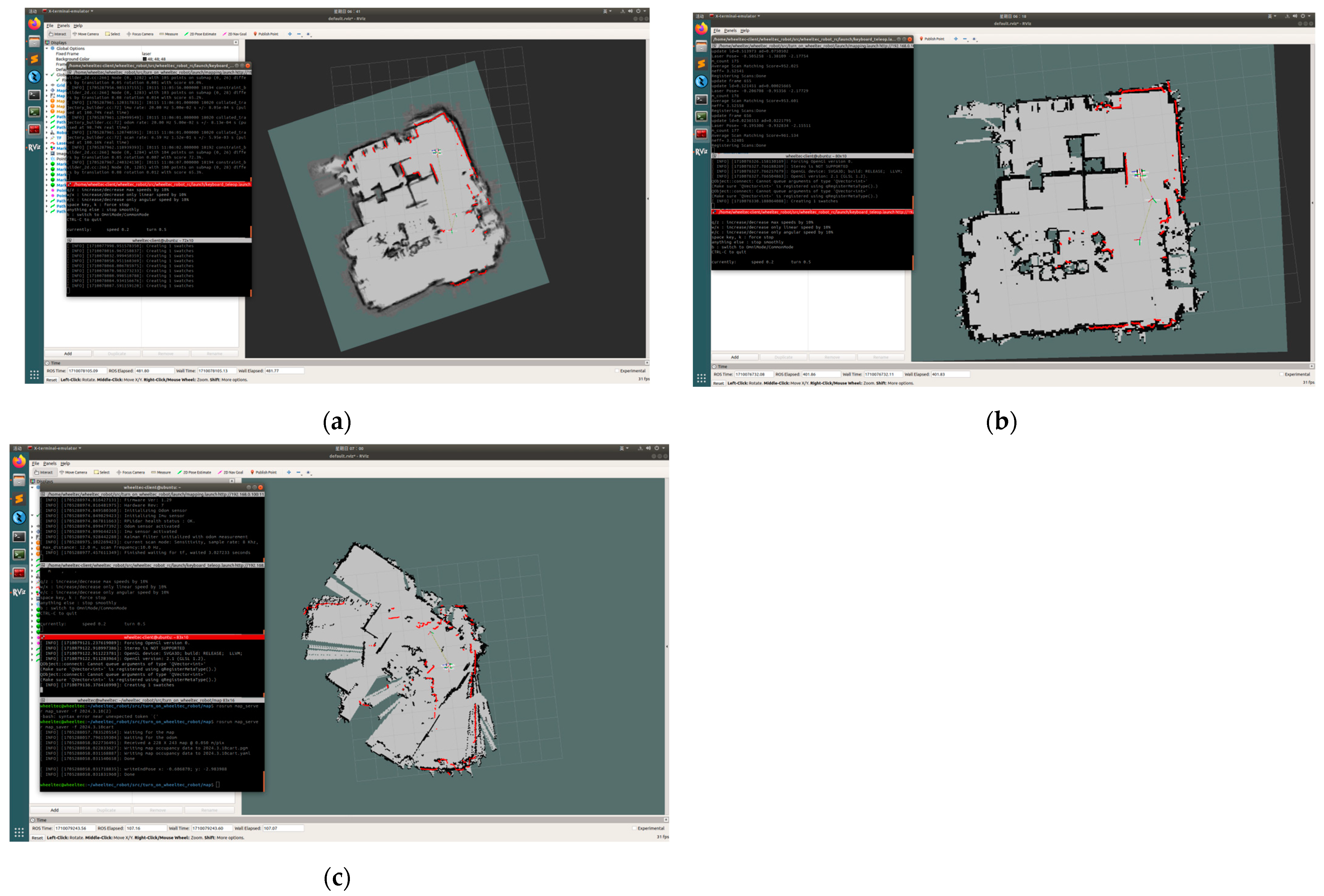
Due to transitioning to an actual office environment, which is inherently more complex than simulated or controlled environments, including potential dead-end areas unreachable by the robot, we conducted the SLAM experiment with the robot moving at a slower, steadier pace. This approach allowed for the collection of more environmental data points, ensuring optimal mapping output quality. By moving slowly and steadily, we aimed to capture a comprehensive representation of the environment, thus ensuring that the mapped output closely reflected the real-world office environment. The construction process of the three algorithms is shown in Figure 21.

Figure 21.
The experimental process diagram of the office site experiment. Three algorithmic mapping processes. Figure (a) shows the construction process of Cartographer, Figure (b) shows the construction process of GMapping, and Figure (c) shows the construction process of Hector-SLAM.
3.5.2. SLAM Office Site Construction Results
The map construction results of the three algorithms are depicted in Figure 22. It is evident that desks and chairs are clearly discernible, and even the tripod in the corner is visible in the map generated by GMapping. The Cartographer algorithm requires IMU-assisted localization and may exhibit slight errors, particularly after minor slippage, with more noise and error at the map edges. Hector-SLAM performs admirably in the initial stages but is susceptible to the deterministic factors of robot motion, leading to error accumulation.

Figure 22.
Output result of experiment in the actual office site. Figure (a) shows the output of Cartographer, Figure (b) shows the output of GMapping, and Figure (c) shows the output of Hector-SLAM.
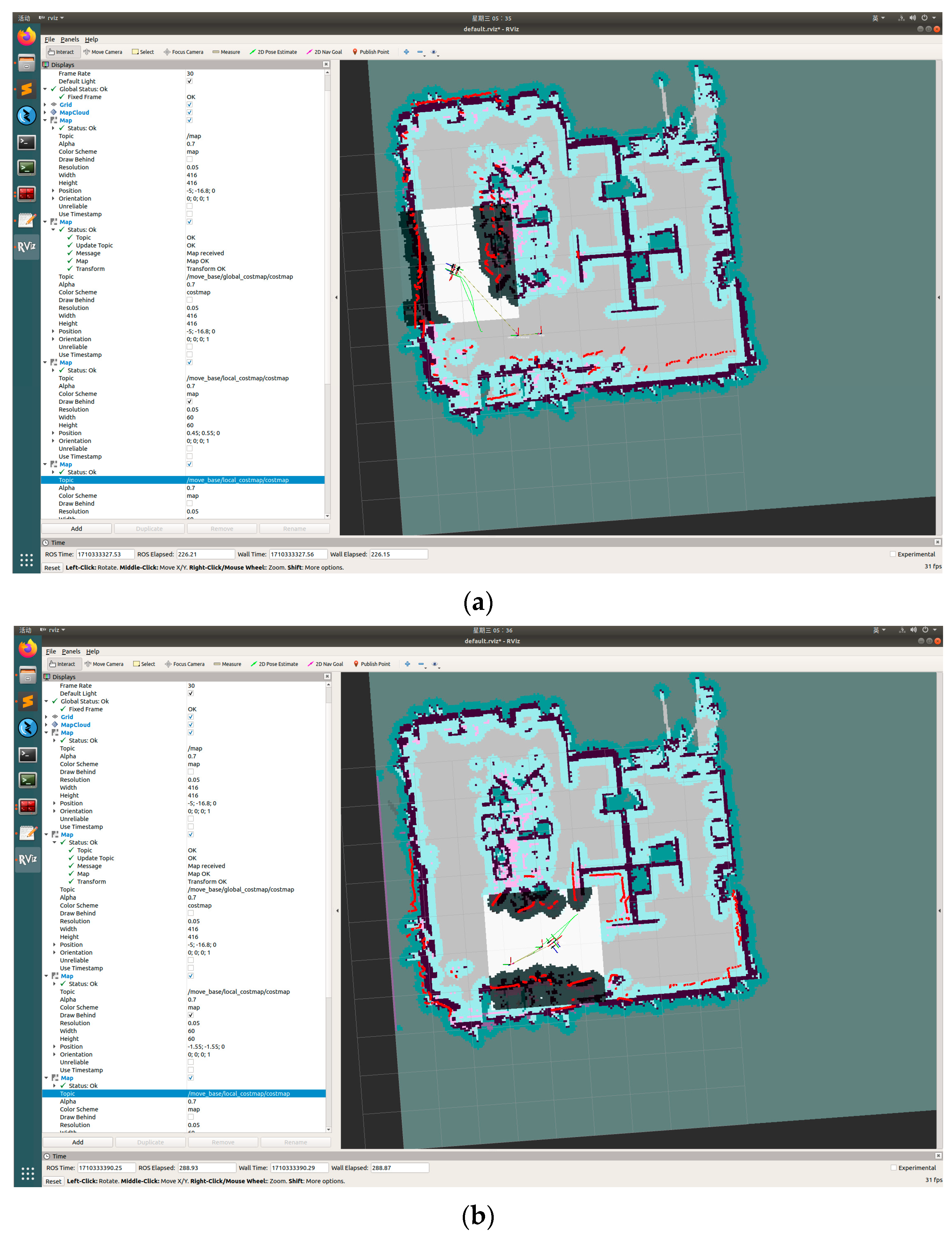
3.5.3. Experiment on Route Planning and Navigation in Office Environment
Figure 23 illustrates the process of path planning and navigation, with the robot successfully plotting a path and navigating to the target point. The clear green path generated during the path-planning process is clearly visible. In the experiment, different target points were selected to demonstrate the effectiveness of path planning in a real office scenario. Despite the presence of various obstacles and complex structures in the office environment, the robot is able to accurately calculate the optimal path to avoid obstacles and successfully navigate to the target point. This indicates that the chosen path-planning algorithm exhibits good applicability and reliability in real-world scenarios, providing a viable solution for autonomous navigation of robots in complex environments.

Figure 23.
Office real-life path planning and navigation diagram. Figure (a) is a randomly selected target point, and Figure (b) is another randomly selected target point different from Figure (a).
3.5.4. Office Site Target Detection
In the office environment, object detection is performed when the robot reaches the target point, identifying small items on the desktop as shown in Figure 24. According to the experimental setup, the recognition algorithm categorizes objects in the image and locates the target objects. In the description, the red box represents the identified office chair with a confidence score of 0.88; the yellow box represents the identified water cup with confidence scores of 0.57 and 0.64 in two separate identifications; the blue box represents the identified pen with a confidence score of 0.58; and the purple box represents the identified glasses with a confidence score of 0.62.
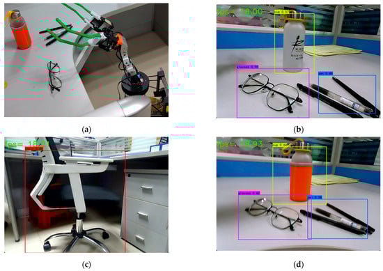
Figure 24.
Picture of the robot performing target detection in a real-life office scene Figure (a) shows the robot in the recognition state. Figure (b) shows the recognized pen, glasses and water cup. Figure (c) shows that the office chair has been identified. Figure (d) shows that the cup (water cup with cup sleeve), water cup, and glasses have been recognized.
3.6. Analysis and Discussion of Experimental Results
3.6.1. Analysis of SLAM and Navigation Experiment Results
Based on the experiments conducted, successful robot path planning and navigation were achieved, with the Dijkstra algorithm employed for global path planning and the teb_local_planner algorithm serving as a crucial component for local path planning. In this process, environmental and pose information was provided by the SLAM mapping system, furnishing the robot with accurate perceptual data. During navigation, the integrity and accuracy of the map are critical factors determining navigation and localization accuracy. Significant errors in map construction often result in localization failures and subsequent navigation inaccuracies [28].
In real-world environments, the practical effects exhibited by the three algorithms differ from those in simulated experiments. The Hector-SLAM algorithm places high demands on LiDAR for turnover rate and measurement noise, presenting certain limitations. Conversely, the Cartographer algorithm requires more computational resources [29].
The unique aspect of the Hector-SLAM algorithm is its independence from odometry information, granting it autonomy. However, in the absence of odometry information, Hector-SLAM is more susceptible to environmental dynamics and uncertainties in robot motion, leading to map drift. Map drift refers to the gradual accumulation of errors during map construction, resulting in inconsistency between the constructed map and the actual environment.
The graph optimization in the Cartographer algorithm exhibits a degree of ambiguity. In real environments, sensor measurements and robot motion may be influenced by noise and uncertainties. These factors may increase the complexity of graph optimization, and its results may be affected by environmental changes and fluctuations in sensor performance. The Cartographer algorithm supports the fusion of multiple sensor data types and performs well in handling large-scale environments, generating accurate maps in complex scenarios. However, it consumes considerable memory and has a large algorithmic footprint. When using high-resolution sensor data, it may lead to significant memory usage and computational load. Moreover, in geometrically symmetric environments, this algorithm is prone to loop closure errors, resulting in inaccurate localization.
In simulated environments, where conditions are idealized, the Hector-SLAM algorithm excels. However, in actual experimental sites, various uncertainties exist. Due to hardware limitations of the robot, the Cartographer algorithm is also not the optimal choice. Throughout the experimental process and in the final output map data, the GMapping algorithm demonstrates excellent performance. Its output maps have clearer boundaries and fewer noise artifacts, outperforming the Hector-SLAM and Cartographer algorithms in indoor mapping performance. Relatively, GMapping excels in real-time indoor map construction, offering relatively lower computational burden and higher accuracy for indoor scene mapping.
3.6.2. Analysis of Experimental Results of Target Detection
YOLOv3 is a lightweight model with fewer parameters and less depth, enabling faster detection processing speed. In our trained dataset, the model performs exceptionally well during experiments. We chose the Adam optimization algorithm to further enhance the accuracy of object detection, which is suitable for running on embedded devices. For instance, in the dataset, identifying pens might pose a challenge because the appearance of pens is closely related to their types and brands in real life, leading to significant differences in appearance among different brands and types of pens. Therefore, the confidence score for identifying pens may be lower compared to other objects. However, even when objects have indistinguishable features or are only partially visible, the model can still identify them with relatively low confidence scores. Improving the comprehensiveness and continuous refinement of the dataset annotations would help enhance recognition accuracy. Despite the presence of multiple small objects or robot movements, the model can accurately identify objects in the dataset.
3.6.3. Discussion
- The applicability and performance of SLAM algorithms vary: In the simulation environment, the Hector-SLAM algorithm excels, but its performance in real-world settings is affected by the accuracy of the LiDAR and measurement noise, leading to suboptimal performance. In contrast, the GMapping algorithm demonstrates greater stability and reliability in real-world environments, with higher localization accuracy. This difference may stem from disparities between the simulation environment and real-world conditions, as well as variations in the algorithms’ sensitivity to sensor accuracy and environmental noise.
- Stability and practicality of SLAM algorithms: The stability and practicality of SLAM algorithms are paramount for ensuring the integrity and accuracy of maps, which directly influence the precision of navigation and localization. Significant errors during map construction can lead to localization failures and inaccurate navigation. Therefore, when selecting a SLAM algorithm, it is crucial to consider the algorithm’s autonomy, reliance on sensor data, and performance under different environmental conditions. The robustness of the algorithm in handling sensor data, managing noise and uncertainty, and maintaining accuracy over time is critical for reliable performance. Evaluating the performance of SLAM algorithms under varied environmental conditions is key. Some algorithms may excel in structured indoor environments but perform poorly in outdoor settings with dynamic lighting and changing terrain. A versatile SLAM algorithm should demonstrate robustness across different scenarios and adapt to challenging conditions encountered in real-world applications. Therefore, when choosing a SLAM algorithm, it is essential to prioritize stability, autonomy, robustness to sensor data, and adaptability to various environmental conditions to ensure that robotic systems can conduct map construction, navigation, and localization accurately and reliably.
- Performance and robustness of object-detection algorithms: The YOLOv3 model performs well in experiments, demonstrating fast processing speed and high recognition accuracy. Although it may face challenges in recognizing objects with significant appearance variations, the model still exhibits robustness and generalization capabilities.
- Directions for future work: SLAM algorithms can be further optimized to enhance their applicability and stability in complex environments, for example, by incorporating additional sensor data or improving algorithm optimization strategies. For object-detection algorithms, continuous refinement of datasets can improve recognition accuracy, especially for objects with significant appearance variations. In practical applications, exploring the integration of different algorithms and technologies can achieve more accurate and reliable indoor service robot systems.
4. Conclusions
This paper delves into the exploration of issues concerning the indoor mobility and identification of service robots. A comparative analysis of the performance of Gmapping, Cartographer, and Hector-SLAM algorithms in experimental environments is conducted. Additionally, the Dijkstra algorithm is employed as the global path-planning algorithm, while the teb_local_planner algorithm serves as the local path-planning algorithm. Through a juxtaposition of simulation and real-world experimental environments, it is convincingly demonstrated that the Gmapping algorithm is better suited to experimental site environments compared to the other two algorithms, owing to its accuracy and adaptability, making it the ideal choice for service robots navigating and identifying objects indoors. However, as the robot operates in different environments, the choice of SLAM algorithm should correspondingly be adjusted to achieve optimal output results. Comparisons, such as those conducted by Pengtao Qu and other scholars, who experimented with three SLAM algorithms in corridors and rooms, concluded that Cartographer exhibited the smallest mapping errors across all experiments, making it the preferred 2D mapping solution compared to other algorithms [30]. This example highlights the varying performance of different SLAM algorithms in different environments. Therefore, it is essential to select an algorithm based on the characteristics of the environment to enable the robot to move and work more efficiently. By choosing the most suitable algorithm for the environment’s features, the robot’s efficiency in movement and tasks can be significantly enhanced. Moreover, the feasibility of the Dijkstra algorithm and teb_local_planner algorithm in path planning is showcased, providing an effective strategy for the motion of service robots.
The utilization of the YOLOv3 algorithm significantly enhances the accuracy of target detection, duly considering the computational capabilities of robot hardware and effectively leveraging device performance. In the selection of optimization algorithms, a comparison is made between the Adam and SGD algorithms. The detection results on the dataset demonstrate that the Adam optimization algorithm outperforms SGD in terms of mAP value, precision, recall, and F1 score. Following meticulous parameter adjustment and comparative experiments, it is confirmed that the Adam optimization algorithm performs better in target detection, with significant advantages in various metrics. For instance, the average precision (AP) of the Adam optimization algorithm on the dataset is 88.04%, whereas that of the SGD algorithm is only 79.16%. These results provide robust support for the selection of excellent target detection models, emphasizing the importance of optimization algorithms for performance and offering valuable guidance for practical applications.
The experimental results indicate that the service robot can significantly enhance work efficiency and facilitate efficient exchange and transfer of items in office or other indoor environments. The deep-learning-based robot vision recognition algorithm provides efficiency in accurately conveying specific objects, showcasing its potential for widespread application in office areas and home environments. Future directions for development should include optimization of robot vision to better understand environmental mapping relationships, thereby demonstrating superior performance in real-world environments. These research findings offer valuable insights into the optimization and improvement of service robots in practical applications.
Author Contributions
Conceptualization, M.L. and B.Z.; methodology, M.L.; software, M.L. and B.Z.; validation, M.C., Z.W. and W.D.; formal analysis, M.L. and B.Z.; investigation, M.L., B.Z. and W.D.; resources, M.C., Z.W. and W.D.; data curation, M.L. and B.Z.; writing—original draft preparation, M.L. and B.Z.; writing—review and editing, M.L., M.C. and Z.W.; visualization, M.L. and B.Z.; supervision, M.C. and Z.W.; project administration, M.L., M.C. and Z.W.; funding acquisition, W.D. All authors have read and agreed to the published version of the manuscript.
Funding
This research was funded by the National College Student Innovation and Entrepreneurship Training Program No. 232310407040X. This project comes from China’s national innovation training program for college students. The project name is SLAM Genie—the leader of unmanned management intelligent robots in university laboratories. The project number is 232310407040X. The project leader is Deng Wangfen, who is also the fifth author of the paper.
Data Availability Statement
The data used to support the findings of this study are available from the corresponding author upon request.
Conflicts of Interest
The authors declare no conflicts of interest.
References
- Niloy, M.A.K.; Shama, A.; Chakrabortty, R.K.; Ryan, M.J.; Badal, F.R.; Tasneem, Z.; Ahamed, H.; Moyeen, S.I.; Das, S.K.; Ali, F.; et al. Critical design and control issues of indoor autonomous mobile robots: A review. IEEE Access 2021, 9, 35338–35370. [Google Scholar] [CrossRef]
- Fragapane, G.; De Koster, R.; Sgarbossa, F.; Strandhagen, J.O. Planning and control of autonomous mobile robots for intralogistics: Literature review and research agenda. Eur. J. Oper. Res. 2021, 294, 405–426. [Google Scholar] [CrossRef]
- Cheong, A.; Lau, M.W.S.; Foo, E.; Hedley, J.; Bo, J.W. Development of a robotic waiter system. IFAC-PapersOnLine 2016, 49, 681–686. [Google Scholar] [CrossRef]
- Guo, P.; Shi, H.; Wang, S.; Tang, L.; Wang, Z. An ROS Architecture for Autonomous Mobile Robots with UCAR Platforms in Smart Restaurants. Machines 2022, 10, 844. [Google Scholar] [CrossRef]
- Fang, G.; Cook, B. A Service Baxter Robot in an Office Environment. In Robotics and Mechatronics, Proceedings of the Fifth IFToMM International Symposium on Robotics & Mechatronics (ISRM 2017), Taipei, Taiwan, 28–30 October 2019; Springer International Publishing: Cham, Switzerland, 2019; pp. 47–56. [Google Scholar] [CrossRef]
- Zhang, X.; Li, J. Research and Innovation in Predictive Remote Control Technology for Mobile Service Robots. Adv. Comput. Signals Syst. 2023, 7, 1–6. [Google Scholar] [CrossRef]
- Kumar, S.J. Application and use of telepresence robots in libraries and information center services: Prospect and challenges. Libr. Hi Tech News 2023, 40, 9–13. [Google Scholar] [CrossRef]
- Ye, Y.; Ma, X.; Zhou, X.; Bao, G.; Wan, W.; Cai, S. Dynamic and Real-Time Object Detection Based on Deep Learning for Home Service Robots. Sensors 2023, 23, 9482. [Google Scholar] [CrossRef] [PubMed]
- Kolhatkar, C.; Wagle, K. Review of SLAM algorithms for indoor mobile robot with LIDAR and RGB-D camera technology. Innov. Electr. Electron. Eng. Proc. ICEEE 2020, 2021, 397–409. [Google Scholar]
- Zhou, Y.; Shi, F.; Chen, J. Design and application of pocket experiment system based on STM32F4. In Proceedings of the 2020 8th International Conference on Information Technology: IoT and Smart City, Xi’an China, 25–27 December 2020; pp. 40–45. [Google Scholar] [CrossRef]
- Moshayedi, A.J.; Roy, A.S.; Liao, L.; Khan, A.S.; Kolahdooz, A.; Eftekhari, A. Design and Development of Foodiebot Robot: From Simulation to Design. IEEE Access 2024, 12, 36148–36172. [Google Scholar] [CrossRef]
- Pebrianto, W.; Mudjirahardjo, P.; Pramono, S.H.; Setyawan, R.A. YOLOv3 with Spatial Pyramid Pooling for Object Detection with Unmanned Aerial Vehicles. arXiv 2023, arXiv:2305.12344. [Google Scholar] [CrossRef]
- Al-Owais, A.; Sharif, M.E.; Ghali, S.; Abu Serdaneh, M.; Belal, O.; Fernini, I. Meteor detection and localization using YOLOv3 and YOLOv4. Neural Comput. Appl. 2023, 35, 15709–15720. [Google Scholar] [CrossRef]
- Li, H.; Liu, L.; Du, J.; Jiang, F.; Guo, F.; Hu, Q.; Fan, L. An improved YOLOv3 for foreign objects detection of transmission lines. IEEE Access 2022, 10, 45620–45628. [Google Scholar] [CrossRef]
- Lawal, M.O. Tomato detection based on modified YOLOv3 framework. Sci. Rep. 2021, 11, 1447. [Google Scholar] [CrossRef]
- Kim, K.; Kim, J.; Lee, H.-G.; Choi, J.; Fan, J.; Joung, J. UAV Chasing Based on YOLOv3 and Object Tracker for Counter UAV Systems. IEEE Access 2023, 11, 34659–34673. [Google Scholar] [CrossRef]
- Wang, H.; Zhang, F.; Liu, X.; Li, Q. Fruit image recognition based on DarkNet-53 and YOLOv3. J. Northeast Norm. Univ. (Nat. Sci. Ed.) 2020, 52, 60–65. [Google Scholar]
- Tian, C.; Liu, H.; Liu, Z.; Li, H.; Wang, Y. Research on multi-sensor fusion SLAM algorithm based on improved gmapping. IEEE Access 2023, 11, 13690–13703. [Google Scholar] [CrossRef]
- Zhang, L.; Wei, L.; Shen, P.; Wei, W.; Zhu, G.; Song, J. Semantic SLAM based on object detection and improved octomap. IEEE Access 2018, 6, 75545–75559. [Google Scholar] [CrossRef]
- Zhang, Y.; Li, R.; Wang, F.; Zhao, W.; Chen, Q.; Zhi, D.; Chen, X.; Jiang, S. An autonomous navigation strategy based on improved hector slam with dynamic weighted a* algorithm. IEEE Access 2023, 11, 79553–79571. [Google Scholar] [CrossRef]
- Xu, J.; Wang, D.; Liao, M.; Shen, W. Research of cartographer graph optimization algorithm based on indoor mobile robot. J. Phys. Conf. Ser. 2020, 1651, 012120. [Google Scholar] [CrossRef]
- Zhang, X.; Lai, J.; Xu, D.; Li, H.; Fu, M. 2d lidar-based slam and path planning for indoor rescue using mobile robots. J. Adv. Transp. 2020, 2020, 8867937. [Google Scholar] [CrossRef]
- Hess, W.; Kohler, D.; Rapp, H.; Andor, D. Real-time loop closure in 2D LIDAR SLAM. In Proceedings of the 2016 IEEE International Conference on Robotics and Automation (ICRA), IEEE, Stockholm, Sweden, 16–21 May 2016; Volume 20, pp. 1271–1278. [Google Scholar] [CrossRef]
- Mi, Z.; Xiao, H.; Huang, C. Path planning of indoor mobile robot based on improved A* algorithm incorporating RRT and JPS. AIP Adv. 2023, 13, 045313. [Google Scholar] [CrossRef]
- Rösmann, C.; Feiten, W.; Wösch, T.; Hoffmann, F.; Bertram, T. Trajectory modification considering dynamic constraints of autonomous robots. In Proceedings of the ROBOTIK 2012; 7th German Conference on Robotics, Munich, Germany, 21–22 May 2012; VDE: Offenbach, Germany, 2012; pp. 1–6. ISBN 978-3-8007-3418-4. [Google Scholar]
- Macenski, S.; Martín, F.; White, R.; Clavero, J.G. The marathon 2: A navigation system. In Proceedings of the 2020 IEEE/RSJ International Conference on Intelligent Robots and Systems (IROS), IEEE, Las Vegas, NV, USA, 24 October 2020–24 January 2021; pp. 2718–2725. [Google Scholar] [CrossRef]
- Guo, J. Research and Optimization of Local Path Planning for Navigation Robots Based on ROS Platform. Mod. Inf. Technol. 2022, 6, 144–148. (In Chinese) [Google Scholar] [CrossRef]
- Zhang, B.; Li, S.; Qiu, J.; You, G.; Qu, L. Application and Research on Improved Adaptive Monte Carlo Localization Algorithm for Automatic Guided Vehicle Fusion with QR Code Navigation. Appl. Sci. 2023, 13, 11913. [Google Scholar] [CrossRef]
- Yong, T.; Shan, J.; Fan, R.; Tianmiao, W.; He, G. An improved Gmapping algorithm based map construction method for indoor mobile robot. High Technol. Lett. 2021, 27, 227–237. [Google Scholar]
- Qu, P.; Su, C.; Wu, H.; Xu, X.; Gao, S.; Zhao, X. Mapping performance comparison of 2D SLAM algorithms based on different sensor combinations. J. Phys. Conf. Ser. 2021, 2024, 012056. [Google Scholar] [CrossRef]


Disclaimer/Publisher’s Note: The statements, opinions and data contained in all publications are solely those of the individual author(s) and contributor(s) and not of MDPI and/or the editor(s). MDPI and/or the editor(s) disclaim responsibility for any injury to people or property resulting from any ideas, methods, instructions or products referred to in the content. |
© 2024 by the authors. Licensee MDPI, Basel, Switzerland. This article is an open access article distributed under the terms and conditions of the Creative Commons Attribution (CC BY) license (https://creativecommons.org/licenses/by/4.0/).