


A Study of Sliding Friction Using an Acoustic Emission and Wavelet-Based Energy Approach


General Engineering Research Institute, Liverpool John Moores University, Byrom Street, Liverpool L3 3AF, UK
*
Author to whom correspondence should be addressed.
Machines 2024, 12(4), 265; https://doi.org/10.3390/machines12040265
Submission received: 8 March 2024
/
Revised: 1 April 2024
/
Accepted: 12 April 2024
/
Published: 16 April 2024
(This article belongs to the Special Issue Innovations in the Design, Simulation, and Manufacturing of Production Systems)
Abstract
:The purpose of this work is to study the mechanism of running-in during friction and to determine the informative parameters characterizing the degree of its completion. During friction, contact interaction of rough surfaces causes various wave phenomena covering a wide range of frequencies, the subsequent frequency analysis can provide information about the sizes of wave sources and thereby clarify the mechanism of interaction between surface roughness. The using of the wavelet transform for processing the signals of audible acoustic emission made it possible to determine the beginning and the end of the change in the frequency ranges of the interaction of roughness. The code developed by the authors was used to analyze the acoustic emission signals by using wavelet energy and entropy criteria. The mother wavelet was chosen by carefully evaluating the effectiveness of 54 preliminary candidates for the mother wavelet from 7 wavelet families, according to three criteria: (1) maximum wavelet energy; (2) Shannon entropy minimum; and (3) maximum energy-to-Shannon entropy ratio.
1. Introduction
The quality and reliability of modern machines are largely determined by the correct consideration in the design of friction characteristics in various critical frictional interfaces. In each friction pair, in the initial period of the process of contact interaction, the geometric parameters of the friction surfaces change so-called running-in or breaking-in [1]. Widespread practice shows that the operation of a friction pair begins only after the completion of the running-in. Therefore, information about the completion of running-in is the most important characteristic of this process.
To date, standard methods for determining the running-in have not yet been developed. Information about the end of the running-in process directly in the process of friction can be obtained only when conducting laboratory tests, for example, according to data on the stabilization of the friction coefficient or stabilization of the temperature in the contact area. Therefore, there is an urgent need to develop methods for directly determining the run-in time at a working facility. One such method can be Acoustic Emission (AE) testing.
The using of ceramic materials in modern friction units further enhances the problem of the relevance of the study of running-in. The fact is that ceramics, having such very useful properties as strength, hardness, high wear resistance, and the ability to work at high temperatures and in an aggressive environment, have a significantly negative property—brittleness. The tendency of ceramics towards unexpected destruction requires the organization of continuous monitoring of their properties during operation. Therefore, the running-in of such materials must be continuously monitored.
An analysis of the literature has shown that when wear-resistant ceramic and brittle materials are used in friction units, the initial stage of the process in dry friction is practically not studied. There are several explanations for this: firstly, because the friction process is non-equilibrium and fast; secondly, access to the contact gap for direct research is difficult; and thirdly, there are no convenient instrumental methods of research. It is obvious that the running-in mechanism has not been sufficiently studied yet, because, first of all, most research is focused purely on applied applications. However, only by understanding the physical causes of the phenomenon can one choose ways to control it over time. In this regard, it is of interest to use the AE method to control the running-in of movable parts.
2. Background
Friction usually accompanies the mechanism of energy dissipation (dissipation) in the process of relative motion of two bodies [2]. Also, as a result of the frictional interaction of the surfaces, the initial values of the roughness and waviness parameters change in such a way that during further work under the same conditions, there is no noticeable change in their values [3]. A high coefficient of friction does not necessarily entail intense wear, since the frictional interaction energy entering the system is divided in different ways. It can be used, for example, for the formation of oxides, the growth of cracks, the formation of grooves, surface heating, and also for the formation of layers of sheared particles. Thus, two systems may have the same coefficients of friction, but one may have more wear than the other [4].
When friction is initiated, there is a certain transitional period called running-in, during which friction and wear rate decrease to their constant values [5]. The term running-in is used mostly in Europe and Great Britain, while in the United States, the term breaking-in is predominantly used [6]. During the running-in process, the surfaces adapt to each other, leading to a more ordered state, lower energy dissipation rates, and exhibit friction-induced self-organization [7]. Practice shows that, despite the large number of currently available criteria for the end of running-in, there are no standard methods for assessing the running-in of machine-building materials [8]. In this regard, it is of interest to use movable mates to control the running-in using the AE method. One of the criteria for the end of running-in is the stabilization of the selected parameters at a certain level [9]. Other indirect methods can be used to determine whether the burn-in is complete, such as the concentration of wear particles in the lubricant, the vibration characteristics in the bearings, and the temperature of the bearing body [6].
Acoustic emission is a natural phenomenon observed by humans from early times. AE is also sometimes called stress wave emission [10]. The oldest natural sources of emission are earthquakes and rock bursts (sudden rock collapse) in mines [11]. The first documented observation of audible acoustic emission was made in the 8th century AD, by Arab alchemist Abu Musa Jabir Ibn Hayyan Al-Azdi, also known by the Latinized name Geber. In his work ‘Summa perfectionis magisterii’, published in Latin in 1545, he described the ‘harsh sound’ of tin (Jupiter) and the ‘sounds much’ of iron (Mars) in forging. In the Middle Ages, tin smelters tested the samples given to them for melting for the presence of impurities by bending them, since the sound emitted when pure tin was bent (the ‘cry of tin’) made it possible to judge the absence of impurities, such as lead or zinc, which reduce the luster of the casting [12]. Classical AE sources are the result of deformation processes: crack growth and plastic deformation. The author [13] argues that there are only a few main sources of AE that generate the characteristic parameter of ultrasound. In his opinion, more complex sources of AE can be the result of a combination of different types of simple sources.
The physical basis of the AE phenomenon during friction is that the frictional interaction causes a dynamic local change in the fields of mechanical stresses in contacting media, which manifests itself in the appearance of stress waves [14] by registering which one can judge the course of processes and their parameters. Widespread studies of AE during friction in the former Soviet Union (USSR) fell at the beginning of the 1980s and are described in the following works [15,16,17,18,19]. Several research papers have been carried out to confirm or disprove the existence of any type of connection between the AE method and friction. For example, in [20], AE was measured in metal samples under conditions of intense sliding friction. This study showed that there is a relationship between dry sliding friction and AE. Also, certain external variables were found, on which the AE count rate depends. The relationship between AE and friction confirms the fact that AE can be used for modern diagnostics of a technical condition.
Methods for analyzing AE signals, depending on the equipment used, can be divided into two main groups: (1) based on the analysis of signal parameters (classical) and (2) based on waveform analysis (quantitative). The reason for the existence of two methods was the rapid development of microelectronics over the past few decades, since it was previously impossible to record and store a large number of waveforms in a relatively short period of time. Both methods are successfully used today [21]. When monitoring AE in real time, the use of temporal (classical) analysis is common. The measured AE parameters in this case are an acoustic emission event; the number of acoustic emission pulses; the acoustic emission count rate; and the maximum amplitude and energy of acoustic emission [10,22]. Using the so-called quantitative AE technology, it is possible to record and store as many signals as needed, along with their shape, by converting the signals from analog to digital form. This method provides better data interpretation capabilities than the previous one, allowing the use of Digital Signal Processing (DSP) techniques to extract the signal from the noise. As a result, it is possible to perform a more comprehensive, but at the same time more time-consuming data analysis, usually performed in post-processing [21].
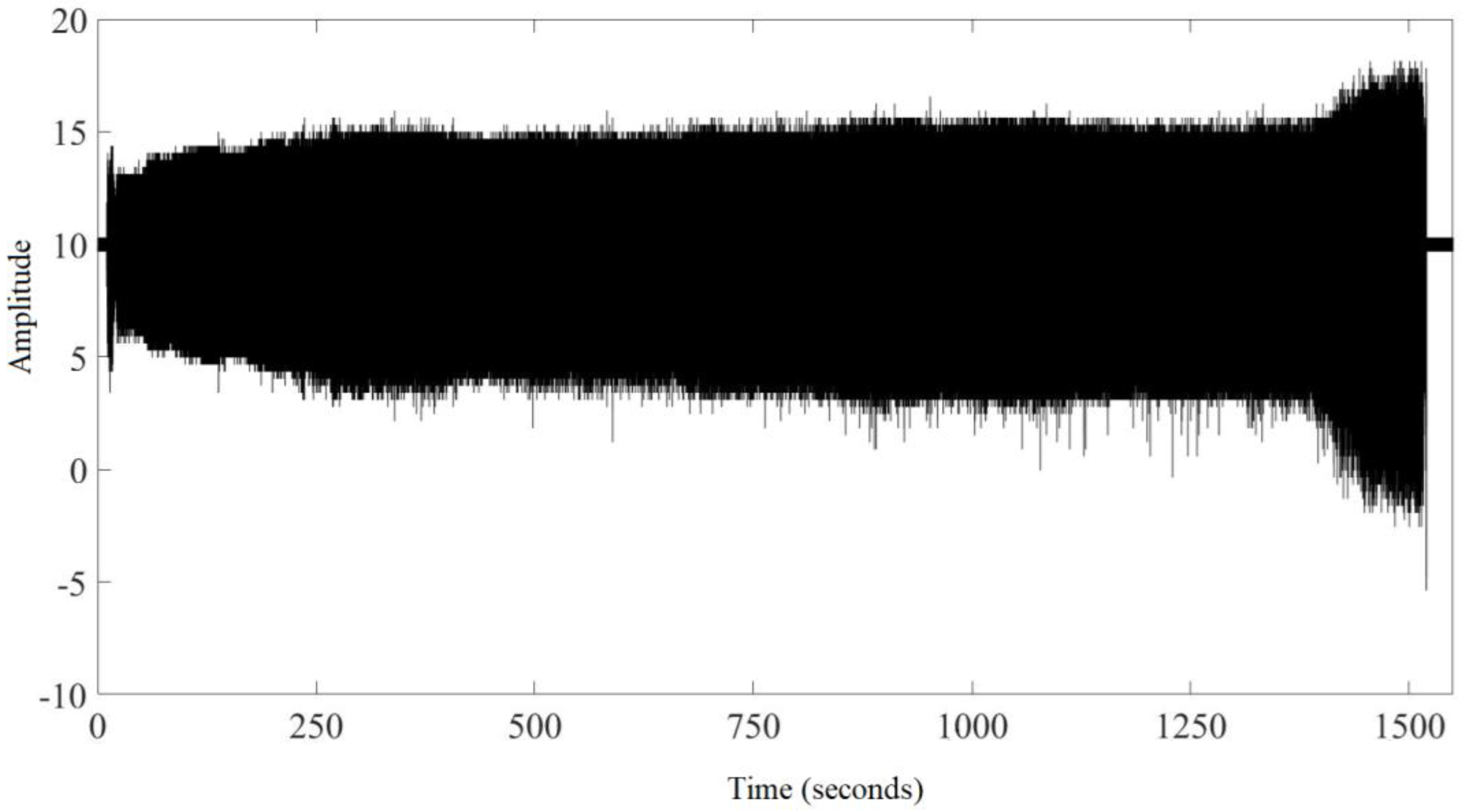
The main disadvantage of the second method is the generation of a large amount of data since the frequency range of AE waves can vary from several Hertz to Megahertz, and, then, in order to cover the weight of this volume of frequencies, in accordance with the Nyquist–Shannon theorem or the sampling theorem, the sampling frequency should be at least twice the maximum signal frequency [23,24]. Due to high sampling rates, signals of even short duration will be large. But, despite this disadvantage, this method is widely used because of its advantages in signal processing. Figure 1 depicts a typical example of the AE signal waveform collected in real time by the AE sensors of the AE monitoring system during friction.
Currently, there are several methods for analyzing waveform-based acoustic emission: (1) amplitude time; (2) frequency; (3) frequency time; and (4) others. The applicability of time or frequency types of analysis is significantly limited for non-stationary signals, which include AE signals; therefore, various time–frequency analysis methods are used [25]: Gabor transform or windowed (local) Fourier transform (FT); Wigner–Ville transform; and wavelet transform (WT). Analysis of the frequency characteristics of signals is usually performed using the Discrete Fourier transform (DFT) and its calculation algorithm, called the Cooley–Tukey algorithm [24]. A modified version of this algorithm, known as the Fast Fourier transform (FFT), mathematically transforms the time domain of AE signals into a sequence of discrete frequency components–spectral analysis. However, the use of the Fourier transform for the spectral analysis of AE signals has two main drawbacks. First, the Fourier transform does not give us any information about the time of occurrence of a particular frequency component. Secondly, the signal must be stationary, which is not suitable for the studied AE signals. One way to overcome these shortcomings is to use the WT as one of the frequency–time analysis techniques. In fact, WT is a timescale method because it transforms a function from the time domain to the timescale domain. WT is a reversible transformation that allows the reconstruction or estimation of certain signal components, even if the inverse transformation may not be orthogonal [26].
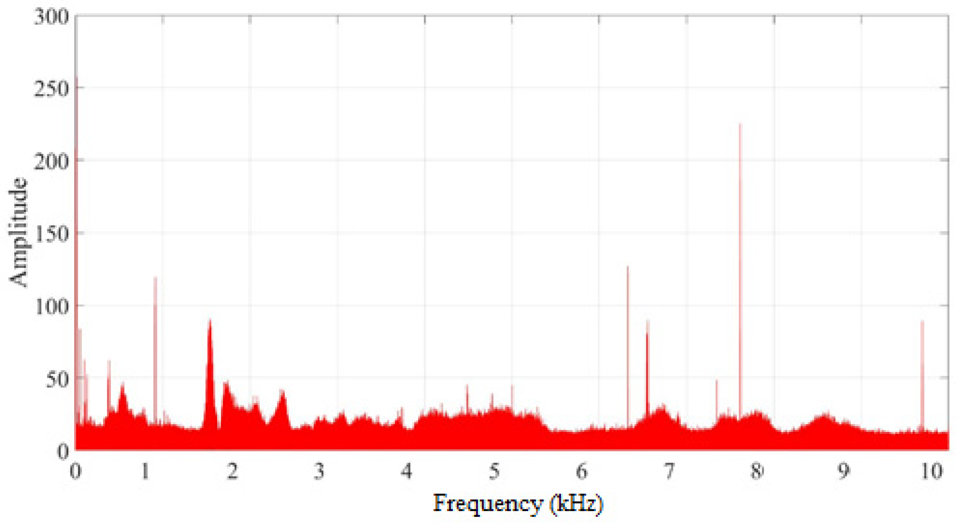
For example, Figure 2 shows the FFT results for a typical raw AE signal. Knowing the frequency range of the AE sensors, we can initially determine the dominant frequency ranges. However, from the presented figure, it is obvious that we cannot unambiguously determine the specific moments in time of the occurrence of one or another frequency component present in the signal. Therefore, in this study, when analyzing AE signals, we concentrate on the criteria of wavelet energy and wavelet entropy, since a different distribution of energy at each frequency component of the signal can be associated with a certain stage of destruction. By analogy with the Fourier transform, wavelet entropy can provide additional useful information underlying the dynamic process of the signal under study.
According to the definition of information entropy introduced by Shannon [27], entropy is a measure of the information of any distribution in the analysis and comparison of probability distributions; that is, it is a measure of the quantitative uncertainty of the system. Moreover, Kolmogorov and Sinai have transformed Shannon’s information theory into a powerful tool for the study of dynamical systems [28,29]. The entropy value of a signal reflects the degree of complexity that the signal has. A more disordered signal shows more entropy. By analogy with the wavelet transform, the wavelet transform-based entropy is called wavelet entropy and can provide additional useful information underlying the dynamic process of the signal under study. This idea is theoretically clarified below.
3. Wavelet Transform
3.1. Introduction
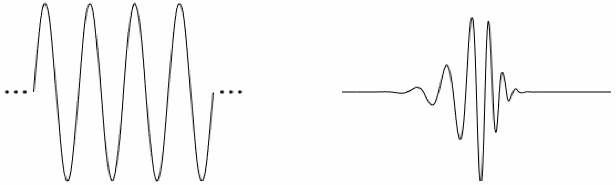
Initially, the term wavelet referred to seismology and was coined by Paul Ricoeur in 1940 to describe the process of disturbance caused by a strong seismic impulse or explosive charge [30]. The English word wavelet is a translation of the French ‘ondelette’, meaning ‘small wave’, originally introduced by A. Grossman and J. Morlet. The basic idea behind wavelet transform signal processing is that a signal can be decomposed into its constituent elements using basis functions. Basis functions can be derived from scaled (expanded) and translated (shifted) versions of a unique generating (mother) function called a ‘wavelet’. The difference between wave and wavelet is in Figure 3.
Mathematically, the wavelet function is defined as follows:
where is the scale parameter (scaling), inversely proportional to the frequency, which determines the frequency and time resolution of the mother (generating) wavelet , ; is the shift parameter (shifting), which determines the position of the wavelet on the -axis, . Wavelets expand when and shrink when . The small scale (high frequencies) corresponds to detailed information about the hidden component of the signal, which usually lasts a relatively short time, while the large scale (low frequencies) corresponds to global information about the signal, which changes slowly. The constant ensures that the norm of these functions is independent of the scaling number for given values of the parameters and [31,32,33].
The wavelet scale is not the same as the Fourier frequency, but it is inversely proportional to the frequency. Therefore, the relationship between the Fourier frequency and the wavelet scale can be approximated as follows:
where is a Fourier frequency, is a central frequency, and is a sampling frequency or sampling rate.
3.2. Continuous Wavelet Transform
There are discrete wavelet transform and continuous wavelet transform, or DWT and CWT, respectively. Unlike the Fourier transform, this is not just a discretization of formulas. The differences between these approaches are deeper; in fact, they can be considered as two different methods for analyzing the structure of signals [34]. The CWT is mainly used for transient analysis, detection of drastic changes in the signal, and investigation of non-stationarity. DWT is most effective in the problems of signal and image compression and cleaning the signal from the background noise [35].
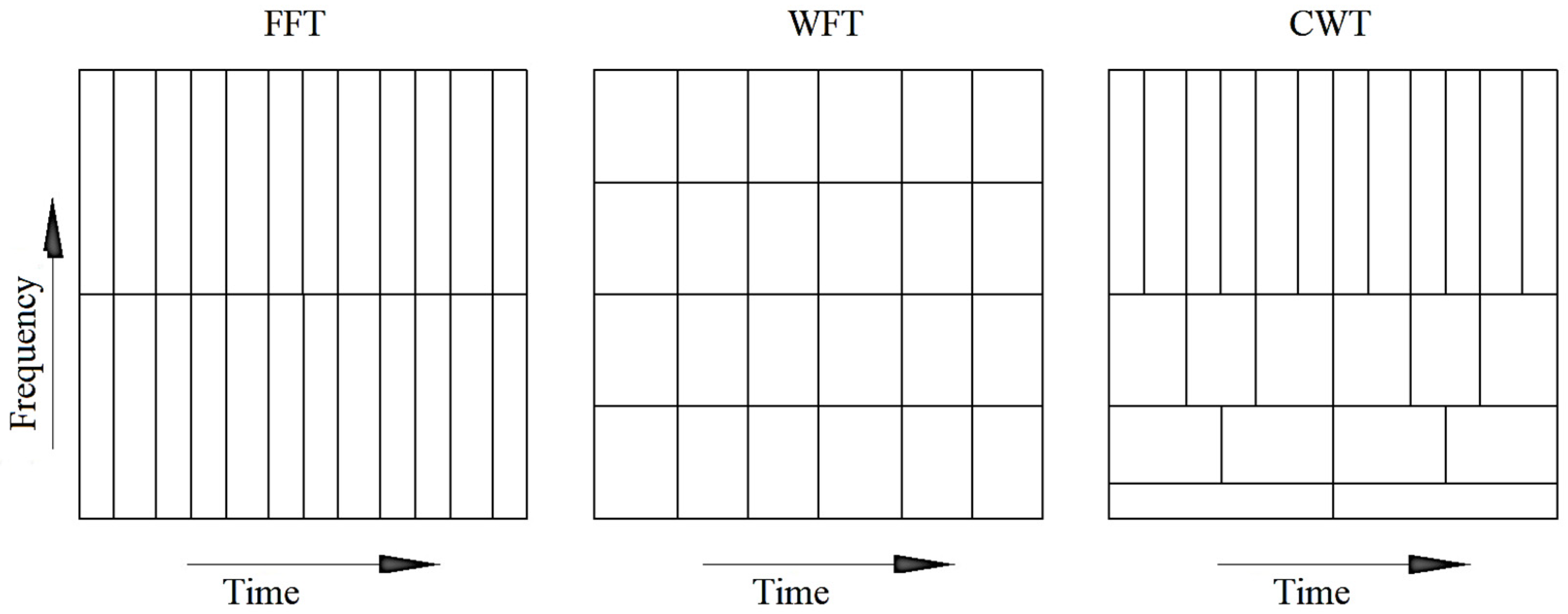
The CWT was developed as an alternative to the Windowed Fourier transform (WFT) in order to overcome the resolution problem that, according to the Heisenberg uncertainty principle or indeterminacy principle, it is impossible to simultaneously know the exact time and frequency of occurrence of a given frequency in a signal [32,36]. In Figure 4, you can see the difference between the frequency and time resolutions of the FFT, WFT, and CWT. Similar to the Gabor transform, the WT uses a variable width time window: a narrow, tall box (high frequencies) means high temporal resolution and a low frequency, and a flat, wide box (low frequencies) symbolizes high partial resolution and low temporal resolution [37]. Thus, a high and accurate time–frequency representation of the analyzed signal is provided.
3.3. Discrete Wavelet Transform
Due to its very strong redundancy, the parameters and are usually discretized, and the discretization performed by a power of two forms a dyadic grid or frames [39]. This kind of CWT is called the discretized wavelet transform [33].
The DWT coefficients are usually sampled from the CWT on a dyadic grid parameter of translation and scale and is defined as follows:
It is not strictly a time–frequency representation but rather a time-scale representation of the signal. WT can give a time–frequency analysis if the center frequency of the wavelet is estimated for each scale.
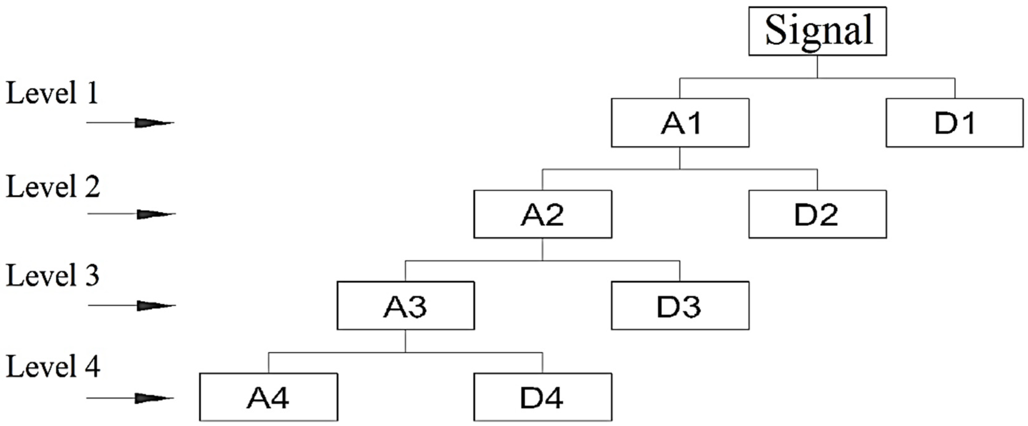
In practice, DWT is implemented using an algorithm known as the Mallat algorithm or the band coding algorithm [40]. When calculating DWT, the original signal is divided into two vectors of coefficients: (1) approximation coefficients and (2) detail coefficients. The first group of coefficients are large-scale, low-frequency components of the signal that serve as input for one of the subsequent iterations, continuing until the desired level of decomposition is reached. The second group of coefficients are small-scale, high-frequency components of the signal. As a result of the decomposition described above, the original signal is a tree structure with wavelet approximations and detail coefficients at various decomposition levels. A schematic graphical representation of the DWT decomposition for 4 levels is shown in Figure 5.
In DWT, decomposition is applied only to approximation coefficients. The restoration of the original signal is performed by summing the detail coefficients of all decomposition levels with the approximation coefficients of the last decomposition level:
where and are the detail and approximation coefficients, respectively.
The maximum number of decomposition levels is directly related to the sampling rate of the analyzed signal. In order to obtain signal details containing frequencies below the frequency , the number of decomposition levels must be taken according to the following [42]:
In the general case, the number of decomposition levels for the wavelet transform is defined as follows:
where is the characteristic frequency component of the signal; is the level of signal decomposition.
Table 1 shows the frequency ranges corresponding to ten levels of DWT decomposition at a sampling rate of 20 kHz and a given signal length that determines the maximum amount of decomposition levels.
Since the characteristic frequency range in the signals we are studying is above the background frequency band created by the working equipment, which is about 50 Hz, the maximum number of decomposition levels is limited to eight.
3.4. Wavelet Energy and Entropy
If is an AE signal, then it can be decomposed into wavelet coefficients. Since the family of functions is an orthonormal basis for the space , the concept of wavelet energy is related to the usual concepts obtained from Fourier theory. For the wavelet coefficients given as , the energy of the detailing coefficients on each time sample is determined by the sum of the squares of the detailing wavelet coefficients of the corresponding decomposition level , :
where is the number of wavelet coefficients and is a wavelet coefficient at level , .
The total signal energy for all decomposition levels is determined by the sum of the energies of all signal decomposition levels:
The relative wavelet energy of the wavelet coefficients at the decomposition levels is calculated by the formula:
The relative wavelet energy provides the relative energy distribution at each decomposition level . Obviously, , and the distribution can be considered as a time-scale density [43].
The concept of wavelet entropy itself follows from the definition of relative wavelet energy and reflects the degree of ordering of the signal under study. For example, a periodic, narrow-band mono-frequency signal can be considered as an ordered process with wavelet energy clearly distinguishable at a single decomposition level containing the characteristic frequency of the signal. For this level, the relative wavelet energy will be almost equal to one, and the wavelet entropy of such a signal will be close to zero or very small, whereas a signal shaped by white noise will demonstrate highly disordered behavior, substantially represented by its frequencies in all frequency ranges. These frequencies are expected to be of the same order and therefore the relative wavelet energies will be almost equal at all levels, thereby generating the wavelet entropy with maximum values.
The total entropy of all wavelet coefficients is defined as the sum of the entropies of all decomposition levels [44]:
3.5. Mother Wavelet Selection
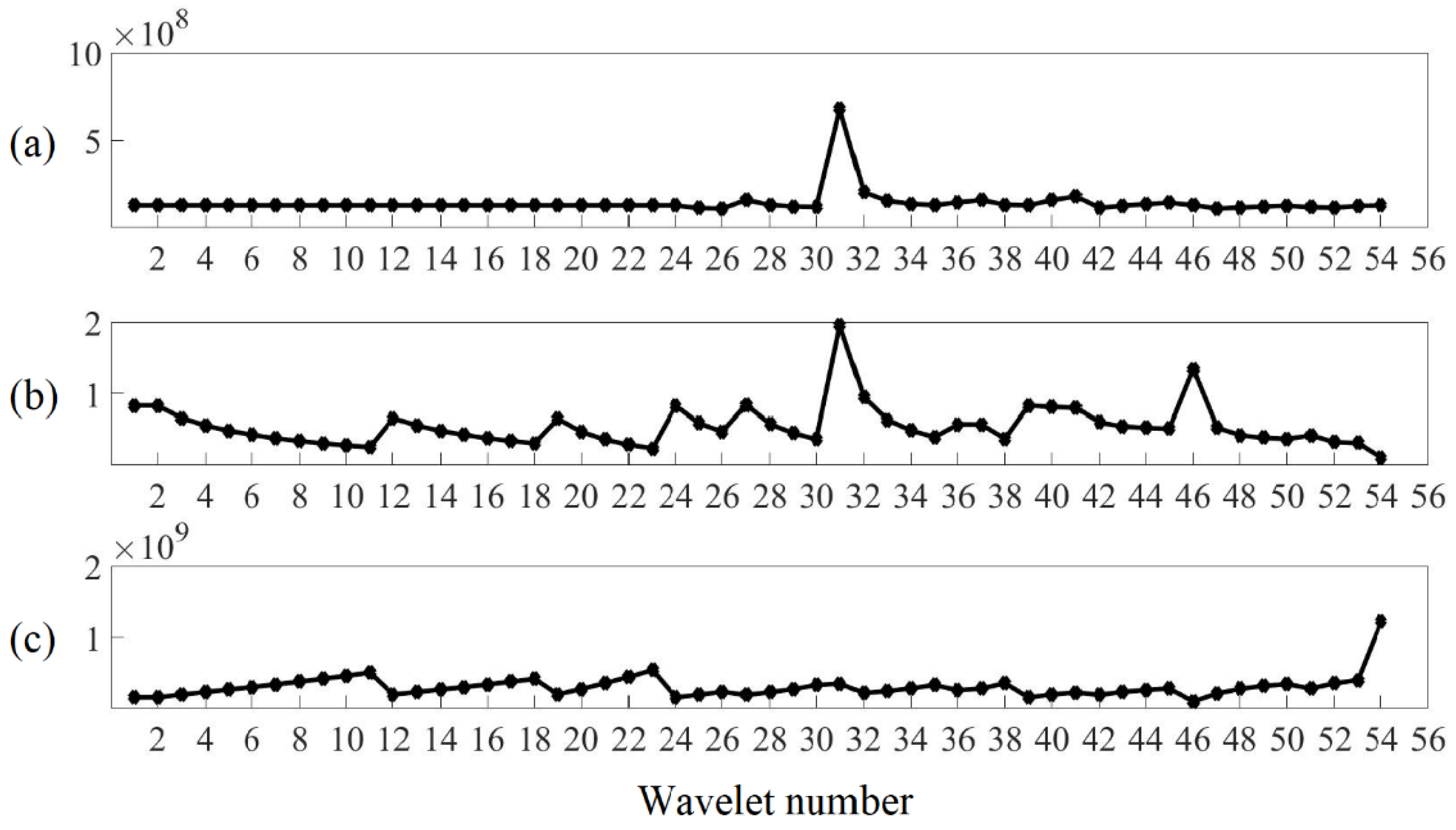
The application of the wavelet transform raises unresolved questions about the choice of the mother wavelet. Different types of wavelets have different time–frequency designs, which causes the problem of choosing the best wavelet function for a particular application. One of the ways to automatically establish the optimal parameters of wavelets is to use the Shannon entropy as a criterion for the analysis and comparison of the probability distribution, which provides a measure of information of any distribution. If the dominant frequency component corresponding to a certain scale parameter is present in the signal under study, then the wavelet coefficients on this scale will have relatively high amplitudes at those times when the dominant frequency component occurs. The energy associated with a given frequency component can be extracted from such a signal using the WT, so the amount of energy can serve as a criterion for choosing the basis wavelet. This concept can be formulated as a criterion for choosing a mother wavelet based on the idea of concentrating the maximum energy of the WT: the basic wavelet that allows you to extract the maximum amount of energy from the analyzed signal is the most suitable wavelet.
The corresponding ordinal numbers of 54 preliminary candidates for the mother wavelet selected from 7 wavelet families are shown in Table 2.
Figure 6a shows that the ‘rbio3.1’ wavelet has the most energy and is considered the most suitable wavelet basis for analyzing AE signals with given parameters. It can also be seen that the amount of energy extracted from the signal increases with the order of the base wavelet for each of the seven wavelet families. This is because higher-order wavelets within the same family have a higher degree of regularity. And, as a result, they are more suitable for extracting energy from AE signals with given parameters than wavelets of the same family, but less ordered.
Expressions (11) and (12) indicate that the entropy of the wavelet coefficients is limited, as follows:
The entropy will be equal to zero if all wavelet coefficients except for one are equal to zero and will be equal to if the probability of energy distribution for all wavelet coefficients is the same, i.e., . It follows from this that the smaller the value of entropy, the higher the concentration of energy. Therefore, a suitable basic wavelet will have a significant amplitude of the wavelet coefficients at several levels of decomposition and an insignificant value at others, thereby leading to the minimum Shannon entropy. The corresponding basis wavelet selection criterion based on Shannon’s entropy minimum criterion can be represented as follows: the basis wavelet minimizing the entropy of the wavelet coefficients is the most appropriate wavelet.
Based on the minimum entropy criterion, the ‘dmey’ wavelet is considered the most suitable basic wavelet (see Figure 6b). However, this result is not consistent with the ‘rbio3.1’ wavelet selected according to the maximum energy criterion. To solve this conflict, the corresponding ratios of energy to entropy are calculated using the following formula:
From the combination of the two previous criteria, it follows that a suitable basic wavelet allows us to extract the maximum amount of energy from the analyzed signal with a minimum of the Shannon entropy of the corresponding wavelet coefficients. This postulate can be formulated as a criterion: the basic wavelet, which has the maximum ratio of energy to Shannon’s entropy, should be chosen as the most suitable wavelet. Figure 6c shows the result of calculating the maximum energy and minimum entropy for 54 potential wavelets, as well as their relationship. As a result, according to the criterion of the maximum ratio of energy to entropy, the ‘dmey’ wavelet designed by Meyer in the mid-1980s x [39] was chosen.
Figure 7 shows the wavelet function and the wavelet scaling function of the selected wavelet.
3.6. Time-Scale Distribution
In order to proceed to the time distribution of the energy and entropy of the wavelet coefficients, the analyzed signal is split into non-overlapping time windows of length . For each time interval ( with , is the number of counts), the corresponding signal values are assigned to the central point of the time window. If we consider the average wavelet energy instead of the total wavelet energy, then at each decomposition level for time window it is defined as follows:
where is the number of wavelet coefficients at the j-th level decomposition contained in the time window .
In order to obtain the time distribution of the average wavelet energy at the j-th level, the decomposition into average values of the time distribution is calculated by the equation:
Then, the total average wavelet energy for all decomposition levels is defined as follows:
As a result, the total average energy of the wavelet coefficients contained in the time window for all decomposition levels can be determined by the following formula:
The relative wavelet energy of the signal is calculated as the ratio between the wavelet energy of each level and the total energy of the signal of the corresponding time window by the following formula:
It is obvious that .
A representative for the whole time interval entropy of the wavelet coefficients in the time window is defined as follows:
The temporal average of wavelet entropy is given by the following:
In consequence, a mean probability distribution representative for the whole time interval can be calculated and the mean probability distribution is given by the following:
with .
The corresponding average wavelet entropy for the whole time interval is as follows:
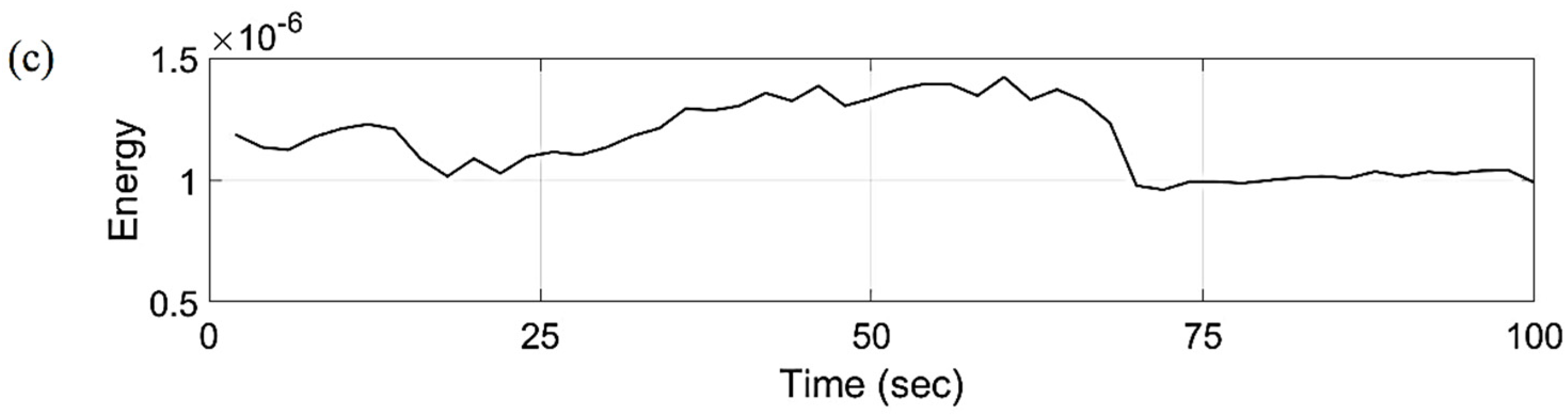
In the applied technique, the length of the window is a very important parameter, and its value directly affects the result of the study. Figure 8 shows a fragment of the wavelet coefficient energy curve for various window lengths. With a small (0.25 s) window length , it will contain a relatively small number of wavelet coefficients inside of the window. As seen in Figure 8a, several peaks and troughs are present over a 100 s time period. It is difficult to isolate the peak or trough corresponding to the actual start time of echo signals. If we take a time window of a relatively large (2 s) length , as shown in Figure 8c, then the energy curve of the wavelet coefficients will be significantly degenerate and the determination of characteristic points in the change in the behavior of the signal under study will cause certain difficulties. Therefore, it is clear that the 1 s window shown in Figure 8b would be the optimal choice for this particular application.
4. Experimental Setup and Test Procedure
4.1. Experimental Setup
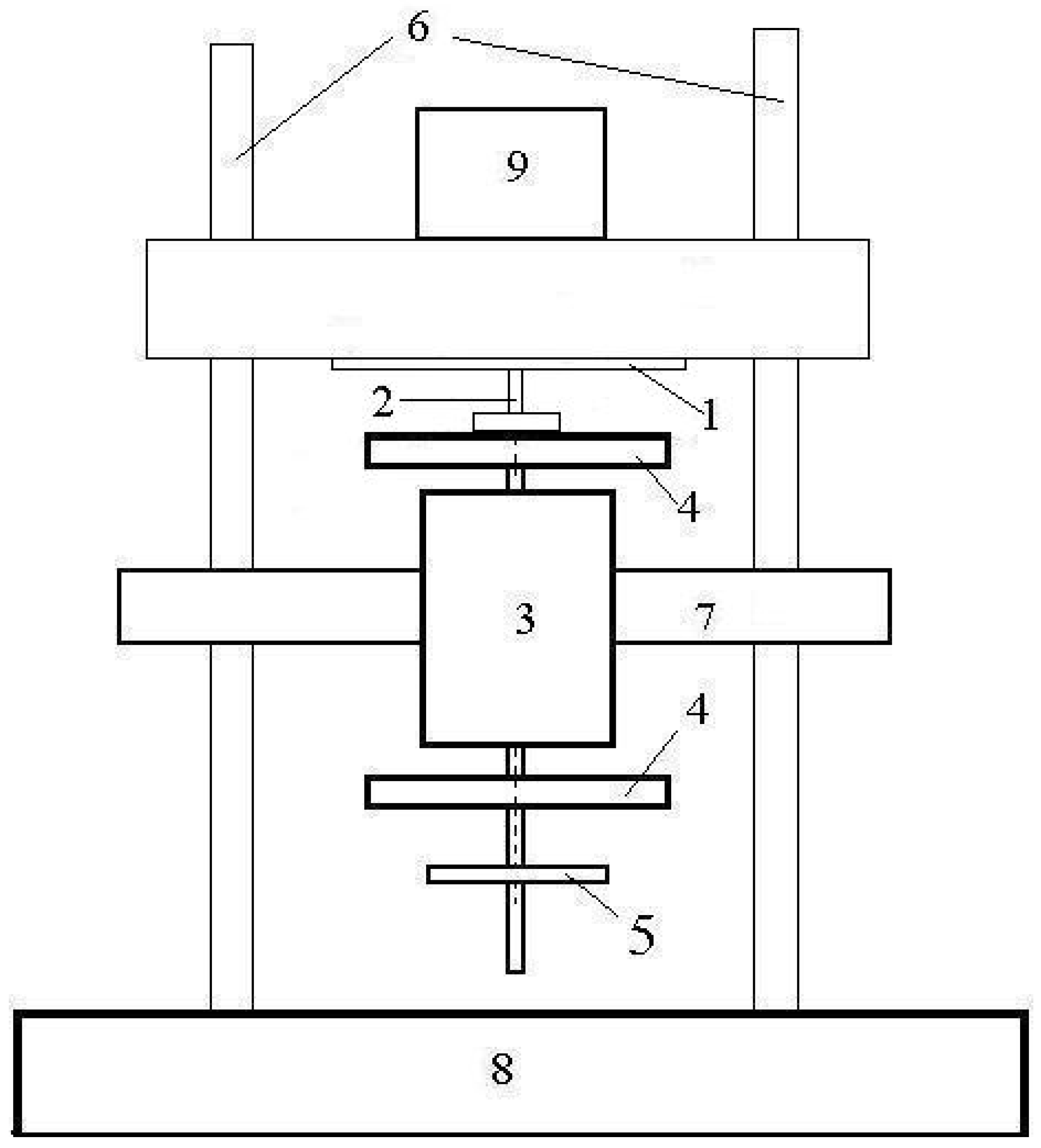
Experimental studies on the study of the initial stage of contact of solids were carried out on various tribological pairs composed of different materials: ceramics, metals, and their combinations. The process of friction of model samples was studied on several types of tribometers operating according to various geometric contact patterns. The variety of materials made it possible to select the optimal model pairs for the respective studies. The choice of equipment and approaches to research is due to the main goal of the work—to obtain information directly during the friction process. The most convenient for friction testing turned out to be a setup with flywheels that was a variant of the movable/fixed ring scheme. It can operate both in continuous mode and under braking conditions. A general view of the installation is shown in Figure 9.
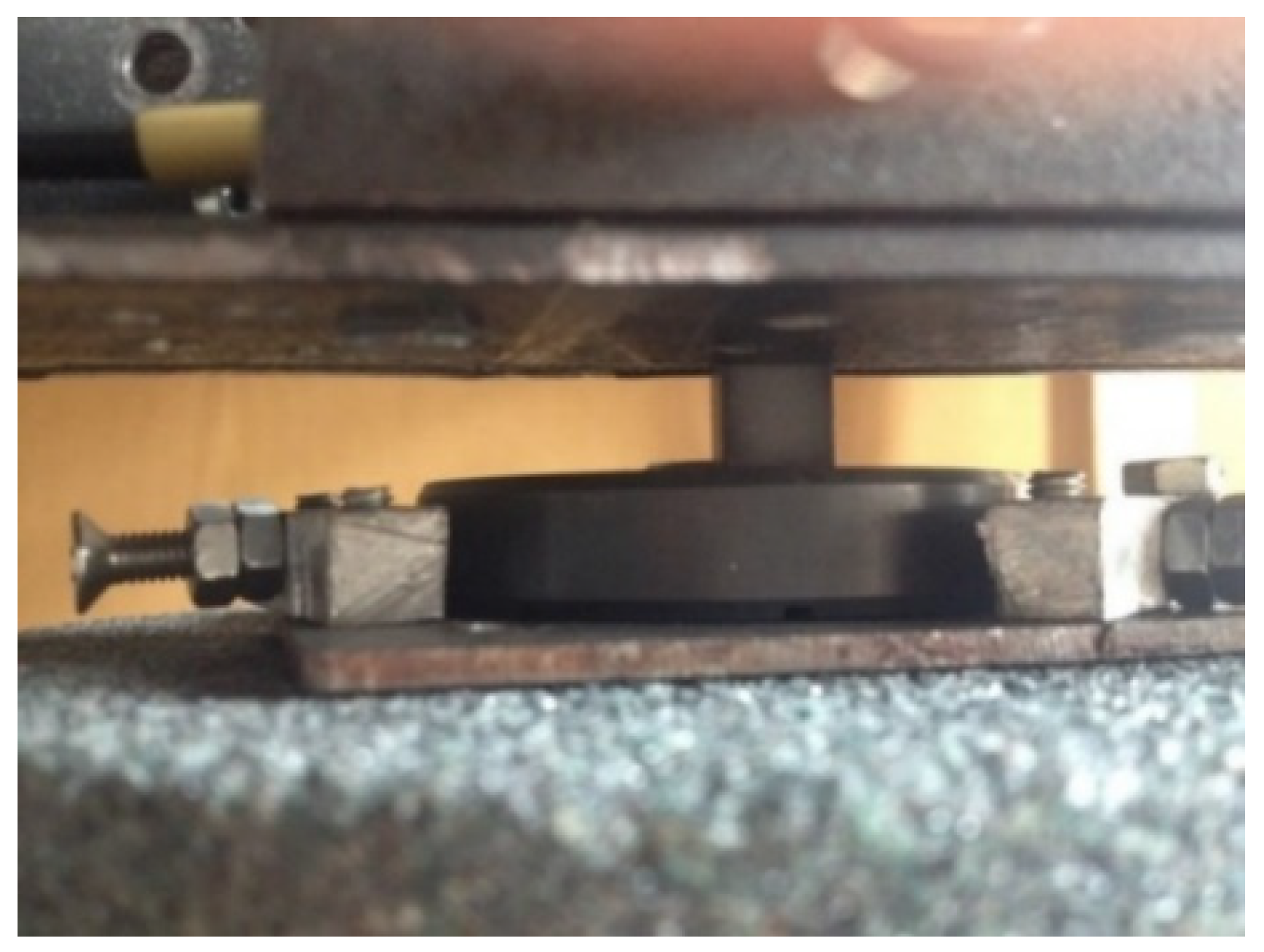
The setup is very effective for rapid express analysis of the tribological properties of materials and testing in liquid media. There are no special requirements for sample dimensions. A movable sample in the form of a disk, rod, ring, tube or even a bar, together with flywheels, can be accelerated by an electric motor up to a maximum angular velocity of 50 rpm. The stationary sample may be in the form of a plate, a ring, a cylinder, or an arbitrary shape with a flat area (see Figure 10). Loads (maximum load 200 N) located on the movable traverse provide contact pressure during friction. The initial deceleration rate, depending on the configuration of the friction pair samples, can reach 25 m/s. During braking, each revolution is registered by a photoelectronic speed sensor. Data from photoelectric sensors, as well as other measuring devices (thermocouples, vibration sensors, microphones, etc.) installed as necessary on the device, are transmitted to the ACK-3107 virtual oscilloscope. When processing data, both the total number of revolutions and the duration of each of them can be determined.
The friction coefficient is calculated using the following formula [45]:
where is the moment of inertia of the rotating masses, is a deceleration path, on which the angular velocity changed from to , and is a load.
4.2. Data Recording and Acquisition
The experimental setup for studying acoustic emission signals consisted of two main instruments. One of the devices was created on the basis of blocks of the standard AF-15 equipment and is designed to record classical high-frequency (HF) acoustic emissions in the range from 200 kHz to 1 MHz, while the other device, on the contrary, provides low-frequency (LF) registration of acoustic signals with a frequency of up to 20 kHz using the ACK-3107 virtual oscilloscope, a personal computer (PC)-based USB oscilloscope, which allows for the recording of the waveform of the AE signal. Each channel of the ACK-3107 has its own analog-to-digital converter (ADC).
The high-frequency path of the installation consisted of a source of wave, a piezoelectric transducer, a preamplifier, a main amplifier, filters and a data processing unit. From the HF processing unit, the AE signal enters the National Instruments PCI-6023e Multifunction I/O DAQ Board, which converts the original analog signal into a sequence of counts. Counts are taken at regular intervals ; this is the so-called sampling period (or interval, sampling step), which is the inverse of sampling frequency () [46,47,48,49]:
At the output of the board, signals event, amplitude, and oscillations are formed. After the event pulse arrives at the computing device, the time of its arrival is determined and a serial number is assigned to it. The amplitude of the AE signal in this work is understood as the maximum value of the amplitude in the radio pulse. This amplitude is measured by a peak detector. Counting the intersections of a certain voltage level by a damped AE pulse gives the signal oscillations. Thus, an array of data is formed in the computer. Based on these data, one can judge how the material wear process changes over time [50].
The low-frequency path consisted of a virtual oscilloscope ACK-3107 and AE sensors of the P113 type made from TsTS-19 piezoceramics, as well as GT-200-01 and GT-205-01. Analogue AE signals arising during the friction were recorded by piezoelectric sensors and transmitted to the ACK-3107 virtual oscilloscope connected to a PC, where they are digitized with a sampling frequency of 20 kHz (see Figure 11), which was determined by the capabilities of the PC.
For experimental registration of wave phenomena, standard acoustic emission equipment is usually used, but if low-pass filters are removed from the amplification path, then the range can be significantly expanded towards lower frequencies. Usually, when using AE to study the destruction of structural materials, they try to avoid the noise of the test equipment and put low-pass filters. In the case of studying the destruction of surface layers of materials during friction, low-frequency interactions are the main ones. It can be assumed that during friction there will be not only wave phenomena associated with the interaction of individual roughness (contact spots), but also larger-scale phenomena associated with the waviness of the surfaces themselves. All this is directly related to the running-in of surfaces.
4.3. Results Correlations and Analysis
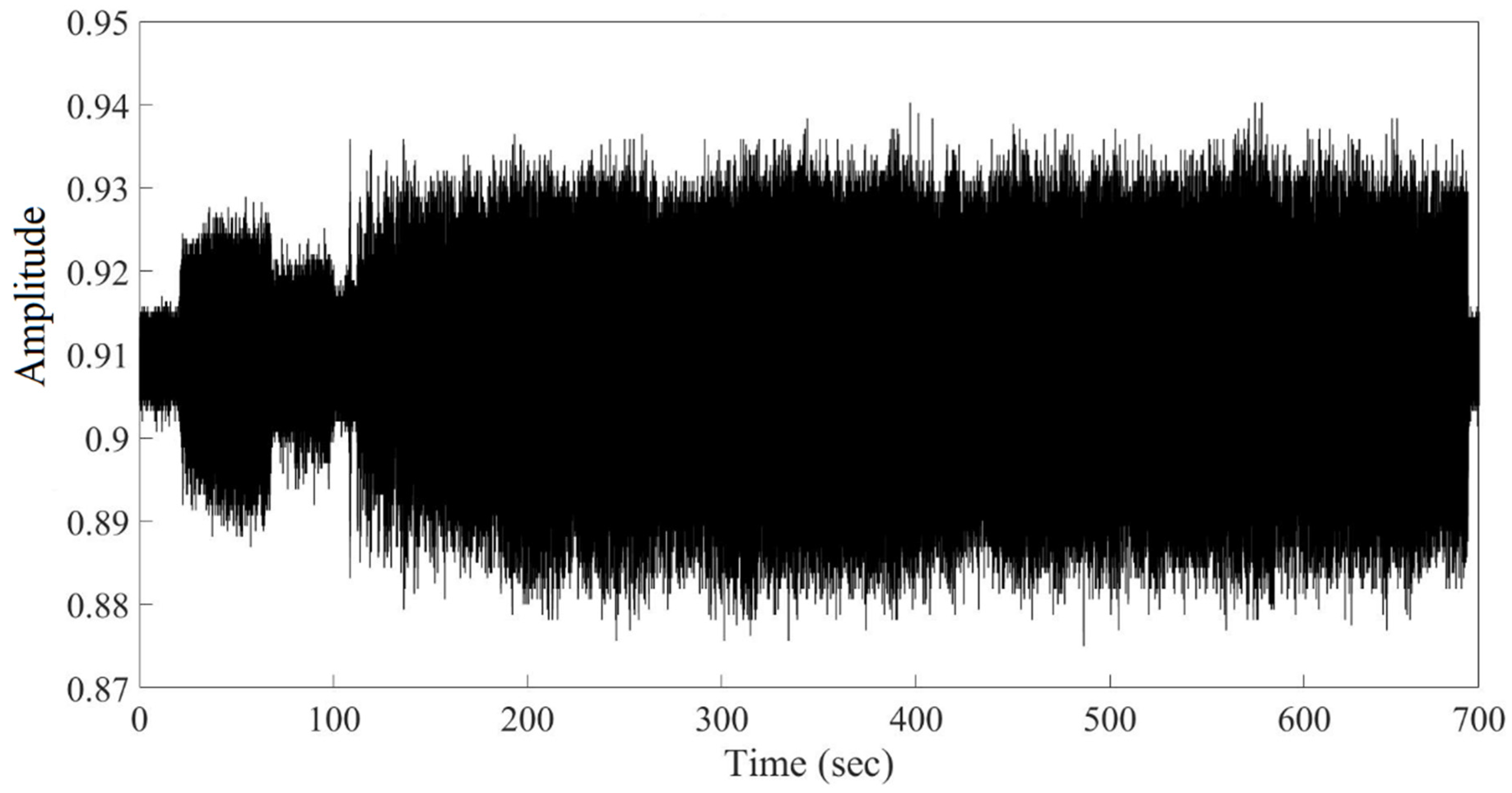
The dry friction behavior of alumina ceramics (Al2O3) against steel was investigated in the air at room temperature, and a constant load of 10 N using the equipment described in Section 4.1. The coefficient of friction calculated by the formula from Section 4.2 was 0.24. To analyze the waveform of the AE signal recorded during the friction (see Figure 12) the MATLAB programming platform was chosen as having numerous options and allowing you to create your own code corresponding to the application. The developed code was used to perform the Fourier transform and wavelet analysis of acoustic emission signals.
Having chosen the mother wavelet (in our case, the Meyer wavelet), the AE signal was decomposed into 8 levels (see Figure 13). The result of the wavelet transform was a sequence of wavelet coefficients at each level of decomposition, ordered by a hierarchical scheme (see the multi-scale analysis described in the previous section). For each moment of time, the wavelet function is related to the waveform of the signal under study at a given position. Such a correlation is a measure of how the position of the wavelet at a given decomposition level corresponds to the waveform signal under study. Each level of decomposition corresponded to a certain frequency range (see Table 3). The results obtained show that the maximum amount of energy is concentrated on the first level, and the energy of the wavelet coefficients contained from levels 4 to 8 is less than 15% of the total energy of the wavelet coefficients of the studied AE signal (see Table 3).
Thus, it is obvious that the maximum amount of information is contained in the first three decomposition levels, which confirms the correctness of the preliminary choice of eight decomposition levels, instead of a maximum possible amount of ten (see Figure 13).
Figure 14 depicts that the initial stage of friction is associated with low-frequency oscillations, which are close to the rotational speed of the tribometer motor and, apparently, are due to the waviness of the rubbing surfaces.
Due to its time–frequency nature, the WT does not show or use frequency responses embedded in the signal resulting from the periodic nature of signal shaping. Therefore, a subsequent spectral analysis of the wavelet coefficients is performed, showing the frequencies hidden in the signal. The spectrum of wavelet coefficients of the decomposed AE signal is shown in Figure 15. Even with a cursory look at the resulting spectrum, several characteristic frequency zones are visible, with their own types of amplitude–frequency characteristics that occur at different periods of the friction process. As shown in Figure 15, the frequency range in the running-in zone is within 1250–2750 Hz. The highest intensity of the spectrum power (100 rel. u.) is in the frequency range of ~1500 Hz. In the zone of stable (steady friction), the frequency range of the AE signal consists of a range of frequencies 2250–5500 Hz with different amplitudes. The highest spectrum power intensity of this frame is twice as low as that of the frame in the running-in area of a tribo unit. Significant changes in the values of the friction coefficient and AE signals are typical for running-in (‘zone 1’, see Figure 15). The increase in the amplitudes of the AE signal is due to the increase in the number of deformation events that occur during running-in, as well as the destruction, separation, and flaking of wear particles in the tribological conjugation zone. In the region of stable friction (‘zone 2’, see Figure 15), small changes in the friction coefficient and the AE signal were registered.
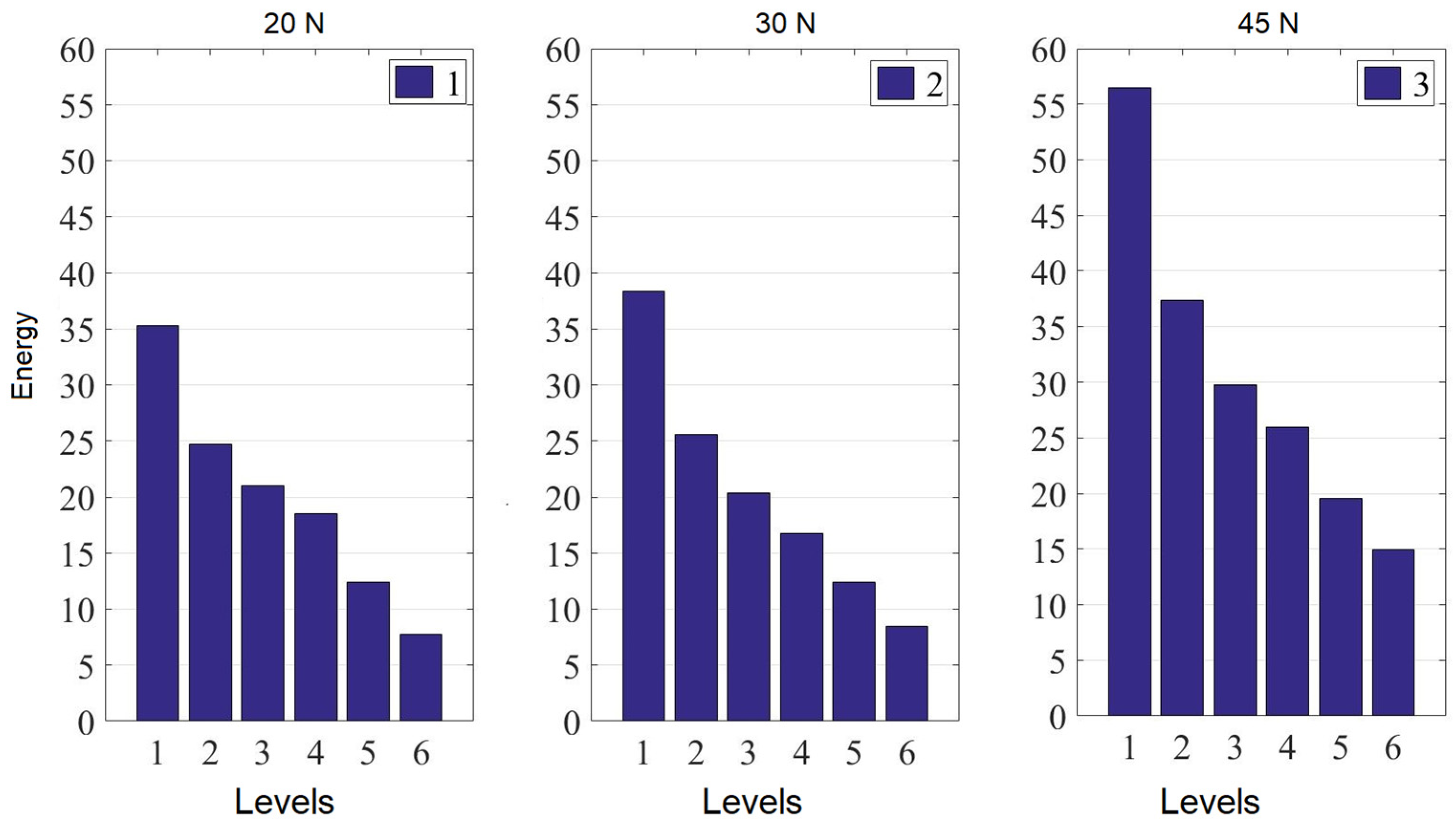
Figure 16 shows the results of calculating the energy distribution of the wavelet coefficients of several AE signals calculated by formulas at various loads. From this figure, it is obvious that a change in the applied load leads to an increase in the energy amplitudes of the wavelet coefficients, while the distribution of the prevailing frequency ranges responsible for certain processes that occur directly in the friction process remains unchanged. This means that the increase in energy caused by the increase in load is absorbed predominantly in the first decomposition level.
5. Further Analysis
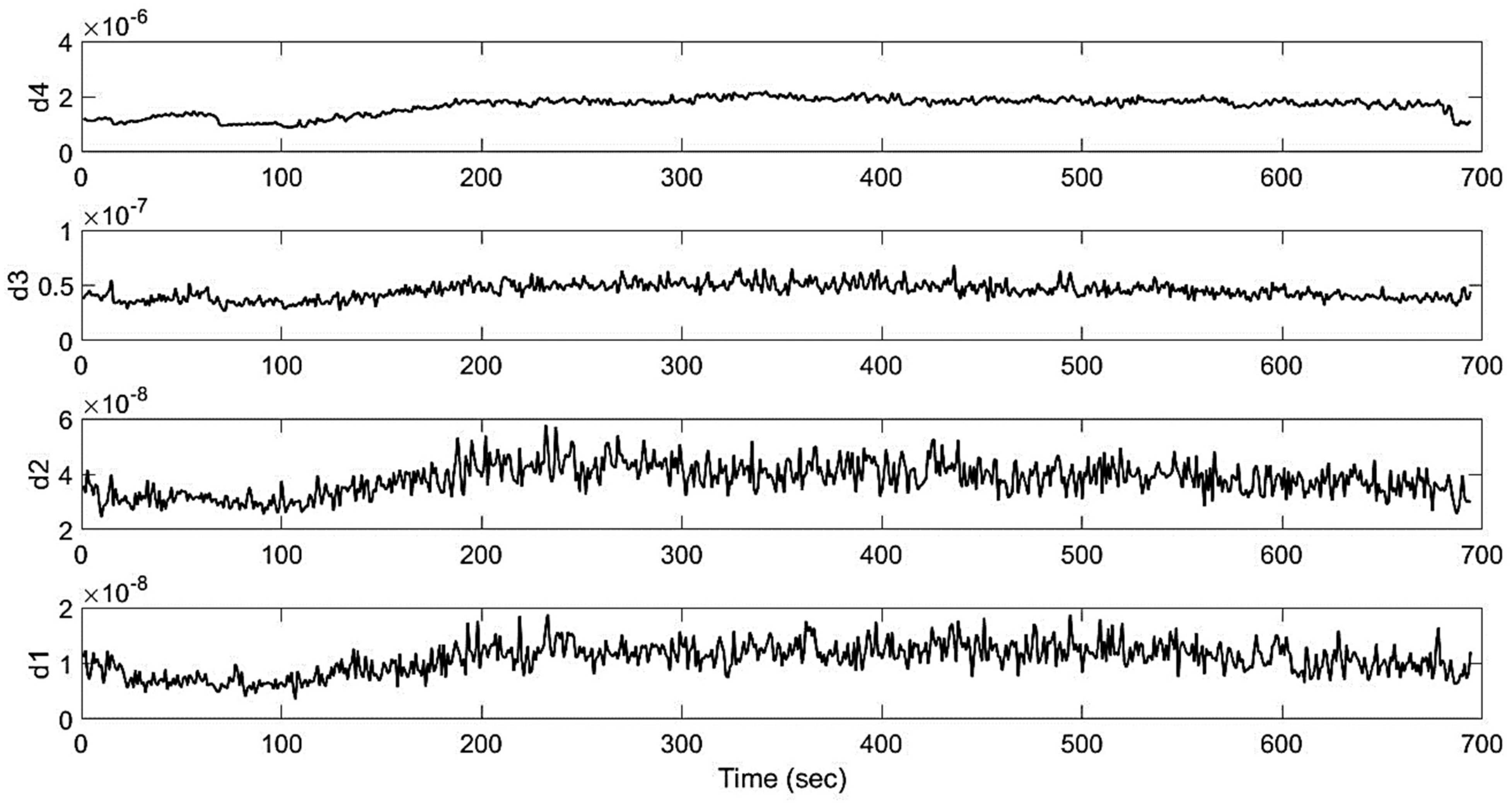
Based on the methodology described in Section 3, the analyzed signal was split into non-overlapping time windows of selected length, namely, 1 s window. Figure 17 shows the distribution of the relative energy of the wavelet coefficients at each scale calculated by formulas from Section 3. In this figure, the vertical coordinates are energy and the horizontal ones are time. As can be seen from this picture, the change in energy distribution differs from one component to another. It is obvious that the energy distribution of different samples under study at the same levels will be different. This difference can be directly related to different failure mechanisms.
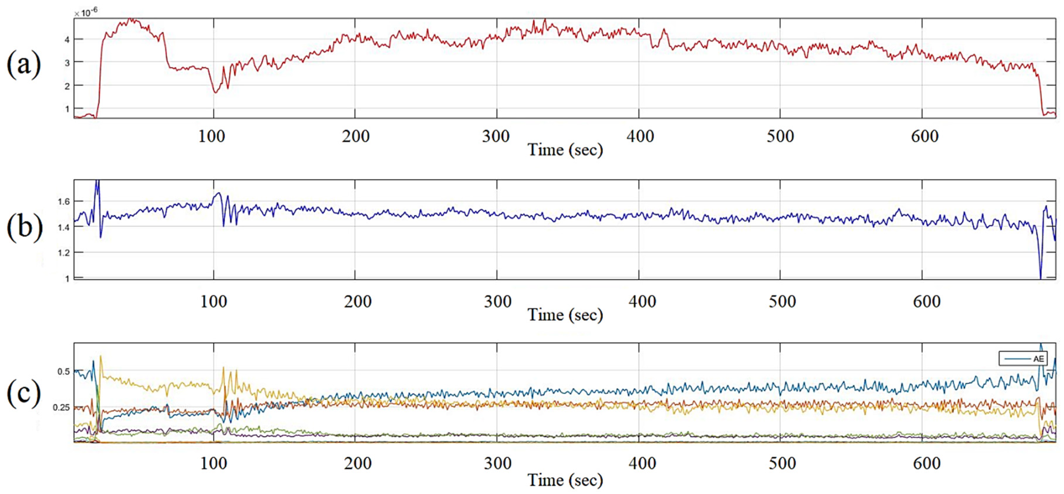
In the following, there is a good correlation between the coefficient of friction and total energy of the wavelet coefficients (see Figure 18), but not between the coefficient of friction and total wavelet entropy of the wavelet coefficients (see Figure 19b). As the irregularities caused by the waviness are removed, the surfaces become more and more smooth, and smaller protrusions come into contact. These protrusions provide a higher AE generation frequency. It is interesting that the moment of time of about 100 s (see Figure 19), corresponding to the end of AE generation at the third level of decomposition (see Figure 15), already goes beyond the stage of a sharp change in the friction coefficient. It can even be said that the friction coefficient has already passed into a stable stage and this corresponds to the traditional ideas about the completion of running-in [1]. In fact, the running-in process continues at a higher structural level and, finally, for this particular example, ends at 200 s (see Figure 19). Further, the detail coefficient takes a stable value.
6. Conclusions
It has been established that during sliding friction of ceramics with speeds less than 10 m/s, the interaction of surface roughness occurs at frequencies up to 5 kHz and is accompanied by audible acoustic emission. The use of a wavelet transform for audible acoustic emission makes it possible to establish the beginning and end of a change in the frequency ranges of roughness interaction. It has been found that by investigating the running-in process using the wavelet transform, one can obtain information about the kinetics of the interaction of roughness of different levels at different points in time.
Spectral analysis of wavelet coefficients can be used to identify zones or stages that occur during friction, in particular, we can talk about the end of running-in. However, further research is needed to understand the reasons for the differences in the frequency spectrum. Thus, it is obvious that the spectral analysis of the wavelet coefficients is more efficient than the traditional Fourier transform or the classical wavelet transform, thereby providing a more detailed visual representation of the change in the frequency characteristics of the AE signal over the entire period of its registration.
The greatest interest is the use of the proposed approach for estimating the surface roughness in the process of friction of practically important brittle materials. Such materials include ceramics, monocrystals, and some types of composites. These materials, as a rule, have a greater hardness than glass, and ground surfaces also have a greater roughness than glass. When tested with such loads as described above, the friction track is not visible under normal observations, and the standard roughness tester is not applicable, while the acoustic emission is fixed quite reliably. Thus, for the first time, it became possible to estimate some friction parameters directly during the experiment.
If the frequency investigation range of the AE signal is not known in advance, then to automate the determination of the sufficiency of decomposition levels, a mathematical criterion based on the criterion for the distribution of the energy of wavelet coefficients can be used. In addition, the use of such mathematical criteria, including the maximum wavelet energy, the Shannon entropy minimum, and the maximum energy-to-Shannon entropy ratio, can be one of the criteria for the automated determination of the optimal mother wavelet, which was demonstrated in this work.
Author Contributions
Conceptualization, S.S. and A.D.L.B.; methodology, S.S.; software, S.S.; validation, S.S. and A.D.L.B.; formal analysis, S.S.; investigation, S.S.; resources, S.S.; data curation, S.S.; writing—original draft preparation, S.S.; writing—review and editing, S.S.; visualization, S.S.; supervision, A.D.L.B.; project administration, A.D.L.B.; funding acquisition, A.D.L.B. All authors have read and agreed to the published version of the manuscript.
Funding
This research received no external funding.
Data Availability Statement
Dataset available on request from the authors.
Acknowledgments
In memoriam Yu. A. Fadin: the authors thank him for his assistance in data acquisition and discussions about wavelet transforms. Yu. A. Fadin Institute of Problems of Mechanical Engineering, Russian Academy of Sciences, St. Petersburg, 199178, Russia.
Conflicts of Interest
The authors declare no conflict of interest.
References
- Kombalov, V.S. Effect of Roughness of Solids on Friction and Wear; Nauka Press: Moscow, Russia, 1974. [Google Scholar]
- Basu, B.; Kalin, M. Tribology of Ceramics and Composites: A Materials Science Perspective; Wiley-American Ceramic Society: Hoboken, NJ, USA, 2011. [Google Scholar]
- Polzer, G.; Meissner, F. Fundamentals of Friction and Wear; Mashinostroenie: Moscow, Russia, 1984. [Google Scholar]
- Blau, P.J. Friction Science and Technology: From Concepts to Applications, 2nd ed.; CRC Press, Taylor & Francis Group: New York, NY, USA, 2009. [Google Scholar]
- Nosonovsky, M. Entropy in Tribology: In the Search for Applications. Entropy 2010, 12, 1345–1390. [Google Scholar] [CrossRef]
- Blau, P.J. On the nature of running-in. Tribol. Int. 2005, 38, 1007–1012. [Google Scholar] [CrossRef]
- Fox-Rabinovich, G.S.; Totten, G.E. Self-Organization during Friction: Advanced Surface-Engineered Materia; CRC Press: Boca Raton, FL, USA, 2019. [Google Scholar]
- Kombalov, V.S. Evaluation of Tribotechnical Properties of Contact Surface; Nauka Press: Moscow, Russia, 1983. [Google Scholar]
- Tur, A.A.; Kholodilov, V. Acoustic-emission diagnostics of the running-in of movable parts. J. Frict. Wear 1987, 8, 546–549. [Google Scholar]
- Mechefske, C.; Sun, G.; Sheasby, J. Using acoustic emission to monitor sliding wear. Insight Non-Destr. Test. Cond. Monit 2002, 44, 490–497. [Google Scholar]
- Malhotra, V.M.; Carino, N.J. Handbook on Nondestructive Testing of Concrete, 2nd ed.; CRC Press: Boca Raton, FL, USA, 2003. [Google Scholar]
- Tensi, H.M. The Kaiser-Effect and Its Scientific Background. J. Acoust. Emiss. 2004, 22, s1–s16. [Google Scholar]
- Scruby, C.B.; Hill, R. Acoustic emission: Theory and practice: Proceedings of the 16th European Working Group on Acoustic Emission Conference. In Proceedings of the 4th European Conference on Non-Destructive Testing, London, UK, 13–17 September 1987; pp. 2831–2838. [Google Scholar]
- Sviridenok, A.I. Acoustic and Electrical Methods in Tribotechnics; Nauka Technika: Minsk, Belarus, 1987. [Google Scholar]
- Svirdenok, A.I.; Kalmykova, T.F.; Kholodilov, V. Investigation of the Actual Area of the Polymer–Metal Friction Contact Using Acoustic Vibrations. J. Frict. Wear 1980, 1, 898–907. [Google Scholar]
- Rapoport, L.S.; Petrov, U.N.; Weinsberg, V.E.; Voronina, N.I. Investigation of the Dynamics of Metal Friction Processes by the Acoustic Emission Method. J. Frict. Wear 1981, 2, 305–309. [Google Scholar]
- Budadin, O.N.; Rapoport, D.A. On the method of automated processing of flaw detection results. Defectoscopia 1982, 3, 531–536. [Google Scholar]
- Filatov, S.V. Acoustic emission during abrasive wear of metals. J. Frict. Wear 1982, 3, 558–562. [Google Scholar]
- Nosovsky, I.G.; Mironov, E.A.; Stadnichenko, N.G. Investigation of the Processes of Deformation and Fracture of Surface Layers of Metals during Friction by the Acoustic Emission Method. J. Frict. Wear 1982, 3, 531–536. [Google Scholar]
- Lingard, S.; Ng, K.K. An investigation of acoustic emission in sliding friction and wear of metals. Wear 1989, 130, 367–379. [Google Scholar] [CrossRef]
- Grosse, C.; Ohtsu, M. Basics for Research—Applications in Civil Engineering. In Acoustic Emission Testing; Springer: Berlin/Heidelberg, Germany, 2008. [Google Scholar]
- Beattie, A.G. Acoustic Emission, Principles and Instrumentation. J. Acoust. Emiss. 1983, 2, 95–128. [Google Scholar]
- Lukin, A. Introduction to Digital Signal Processing; Nauka Press: Moscow, Russia, 2002. [Google Scholar]
- Gao, R.X.; Yan, R. Wavelets; Springer US: Boston, MA, USA, 2011. [Google Scholar] [CrossRef]
- Li, X. A brief review: Acoustic emission method for tool wear monitoring during turning. Int. J. Mach. Tools Manuf. 2002, 42, 157–165. [Google Scholar] [CrossRef]
- Loutas, T.H.; Kostopoulos, V.; Ramirez-Jimenez, C.; Pharaoh, M. Damage evolution in center-holed glass/polyester composites under quasi-static loading using time/frequency analysis of acoustic emission monitored waveforms. Compos. Sci. Technol. 2006, 66, 1366–1375. [Google Scholar] [CrossRef]
- Shannon, C.E. A Mathematical Theory of Communication. Bell Syst. Tech. J. 1948, 27, 379–423. [Google Scholar] [CrossRef]
- Kolmogorov, A.N. A new metric invariant of transitive dynamical systems and of automorphisms of Lebesgue spaces (Russian). Dokl. Akad. Nauk 1958, 119, 861–864. [Google Scholar]
- Sinai, Y.G. On the concept of entropy for a dynamic system: § 1, § 2. Dokl. Acad. Sci. 1959, 124, 768–771. [Google Scholar]
- Stollnitz, E.J.; DeRose, T.D.; Salesin, D.H. Wavelets for Computer Graphics; NIC RHD: Izhevsk, Russia, 2002. [Google Scholar]
- Yakovlev, A.N. Introduction to Wavelet Transform: Tutorial; HGTU: Novosibirsk, Russia, 2003. [Google Scholar]
- Polikar, R. The Story of Wavelets. In Physics and Modern Topics in Mechanical and Electrical Engineering; Mastorakis, N., Ed.; World Scientific and Engineering Society Press: Athens, Greece, 1999; pp. 192–197. [Google Scholar]
- Mallat, S. A Wavelet Tour of Signal Processing; Academic Press: Amsterdam, The Netherlands, 1999. [Google Scholar]
- Yudin, M.N.; Farkov, Y.A.; Filatov, D.M. Introduction to wavelet analysis. In Educational and Practical Guide for the System of Distance Education; MGRI: Moscow, Russia, 2001. [Google Scholar]
- Boriskevich, A.A.; Gursky, A.L.; Kochubeev, Y.G. MPEG Video Compression and Encryption; BGUIR: Minsk, Belarus, 2004. [Google Scholar]
- Cohen, L. Time-frequency distributions—A review. Proc. IEEE 1989, 77, 941–981. [Google Scholar] [CrossRef]
- Goswami, J.C.; Chan, A.K. Fundamentals of Wavelets: Theory, Algorithms, and Applications, 2nd ed.; Wiley-Interscience: New York, NY, USA, 2010. [Google Scholar]
- Hauswirth, I. FFT-1/n-Octave Analysis-Wavelet; Technical Report Application Note-02/18; HEAD Acoustics: Brighton, MI, USA, 2018. [Google Scholar]
- Daubechies, I. Ten Lectures on Wavelets; SIAM: Philadelphia, PA, USA, 1992. [Google Scholar] [CrossRef]
- Mallat, S.G. A theory for multiresolution signal decomposition: The wavelet representation. IEEE Trans. Pattern Anal. Mach. Intell. 1989, 11, 674–693. [Google Scholar] [CrossRef]
- Refahi Oskouei, A. Wavelet-based acoustic emission characterization of damage mechanism in composite materials under mode I delamination at different interfaces. Express Polym. Lett. 2009; 3, 804–813. [Google Scholar] [CrossRef]
- Dyakonov, V.P. Wavelets: From the Theory to the Practice, 2nd ed.; CSLON-R: Moscow, Russia, 2010. [Google Scholar]
- Rosso, O.; Blanco, S.; Yordanova, J.; Figliola, A.; Schürmann, M.; Basar, E. Wavelet entropy: A new tool for analysis of short duration brain electrical signals. J. Neurosci. Methods 2001, 105, 65–75. [Google Scholar] [CrossRef]
- Blanco, S.; Figliola, A.; Quiroga, R.Q.; Rosso, O.A.; Serrano, E. Time-frequency analysis of electroencephalogram series III. Wavelet packets and information cost function. Phys. Rev. E 1998, 57, 932–940. [Google Scholar] [CrossRef] [PubMed]
- Kragelsky, I.V.; Vinogradova, I.E. The Coefficients of Friction; Mashgiz: Moscow, Russia, 1962. [Google Scholar]
- Oppenheim, A.V.; Schafer, R.W. Digital Signal Processing; Prentice-Hall: Englewood Cliffs, NJ, USA, 1975. [Google Scholar]
- Antoniou, A. Digital Filters: Analysis and Design (Communications and Information Theory); McGraw-Hill Education: Berkshire, UK, 1979. [Google Scholar]
- Sergienko, A.B. Digital Signal Processing, 2nd ed.; Piter: St. Petersburg, FL, USA, 2007. [Google Scholar]
- Baskakov, S.I. Radio Engineering Circuits and Signals: A Guide to solving problems. In Textbook for High Schools; Vysshaya Shkola: Moscow, Russia, 1983. [Google Scholar]
- Fadin, Y.A. Application of acoustic emissions for mass wear analysis. J. Frict. Wear 2008, 29, 21–23. [Google Scholar] [CrossRef]
Figure 1.
A typical waveform of raw signal AE recorded during the friction.

Figure 2.
Frequency analysis of the raw AE signal.

Figure 3.
Schematic illustration of the difference between a wave (left) and a wavelet (right).

Figure 4.
Frequency and time resolution of the wavelet analysis compared to FFT [38].
Figure 4.
Frequency and time resolution of the wavelet analysis compared to FFT [38].

Figure 5.
Structure tree of the 4-level decomposition [41].
Figure 5.
Structure tree of the 4-level decomposition [41].

Figure 6.
(a) minimum entropy criterion; (b) maximum energy criterion; (c) maximum ratio of energy to Shannon’s entropy criterion.
Figure 6.
(a) minimum entropy criterion; (b) maximum energy criterion; (c) maximum ratio of energy to Shannon’s entropy criterion.

Figure 7.
Meyer scaling function and Meyer wavelet function [39].
Figure 7.
Meyer scaling function and Meyer wavelet function [39].
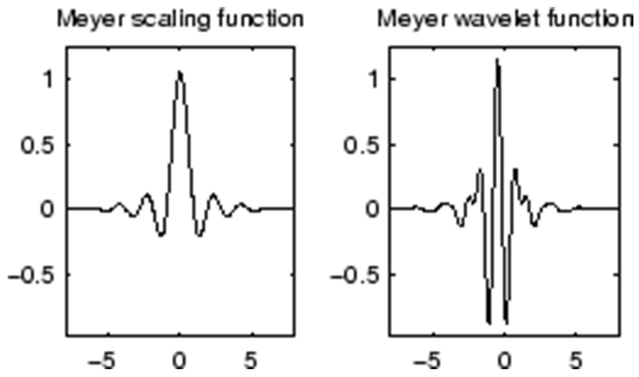
Figure 8.
The length of the window: (a) 0.25 s; (b) 1 s; (c) 2 s.
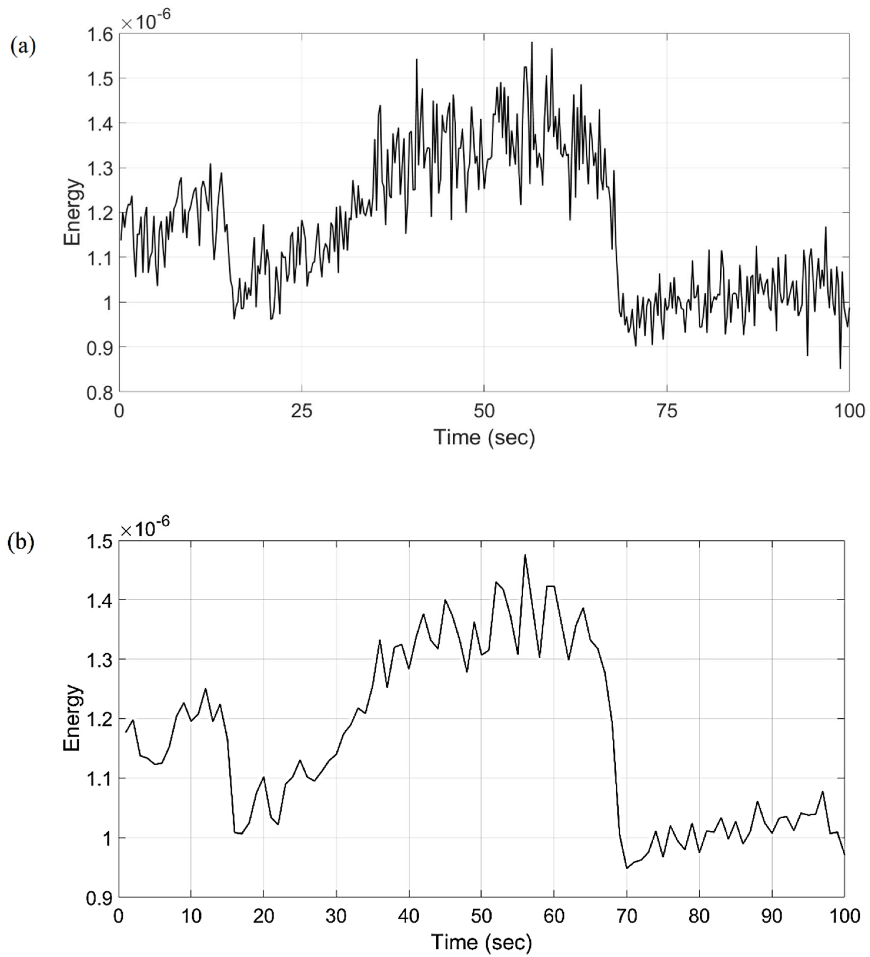

Figure 9.
Experimental setup for the study of friction: 1—stationary sample of the material under study; 2—rotating specimen; 3—electromotor; 4—flywheels; 5—photoelectric speed sensor; 6—guides; 7—motor mount; 8—frame; 9—load.
Figure 9.
Experimental setup for the study of friction: 1—stationary sample of the material under study; 2—rotating specimen; 3—electromotor; 4—flywheels; 5—photoelectric speed sensor; 6—guides; 7—motor mount; 8—frame; 9—load.

Figure 10.
Friction unit: movable sample is a disk; fixed sample is a pin.

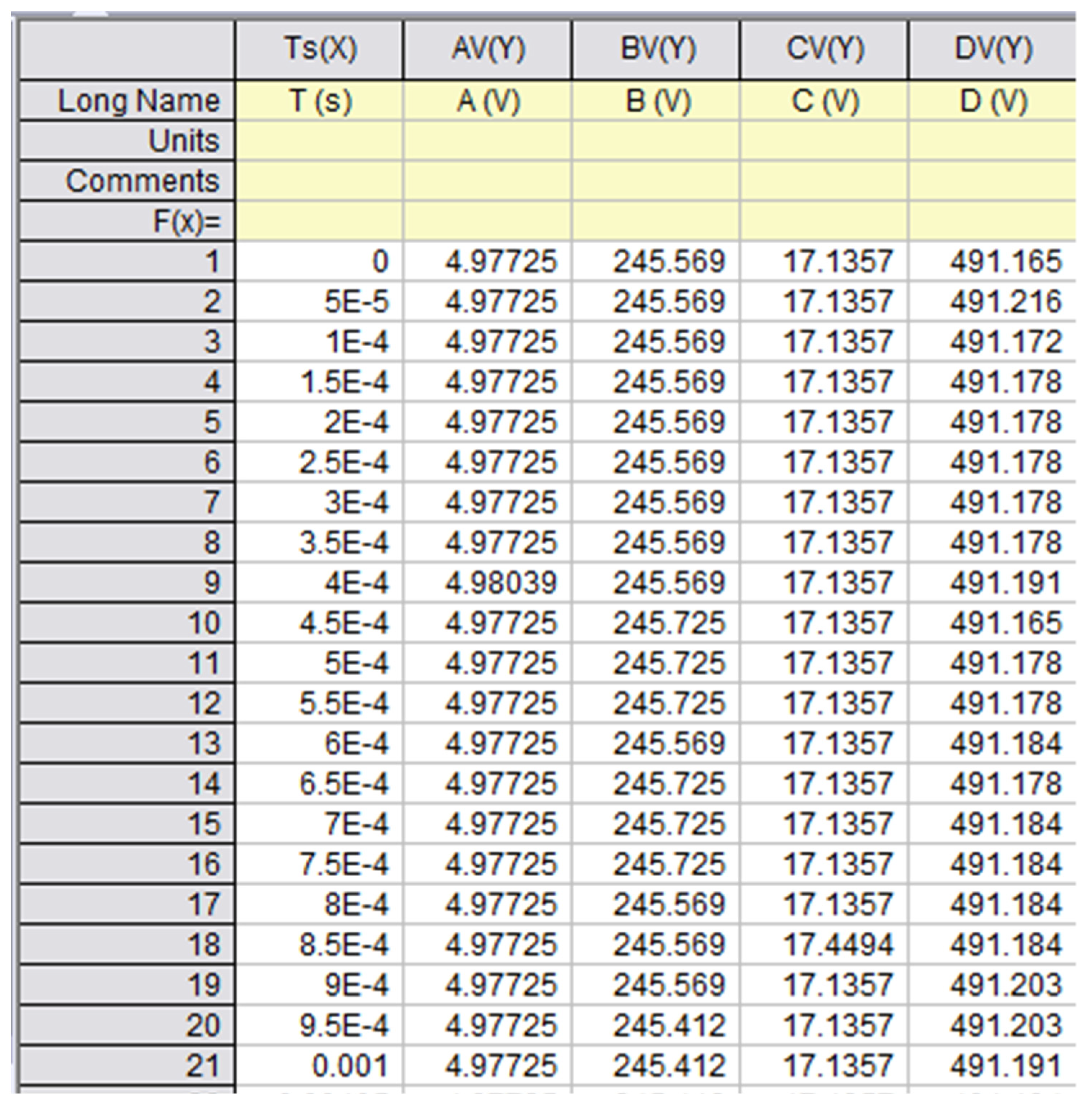
Figure 11.
Fragment of raw AE data collected using ACK-3107.

Figure 12.
Original waveform of AE signal recorded during the friction (amplitude vs. time).

Figure 13.
Histogram of the AE energies at each frequency band for each of decomposition levels.
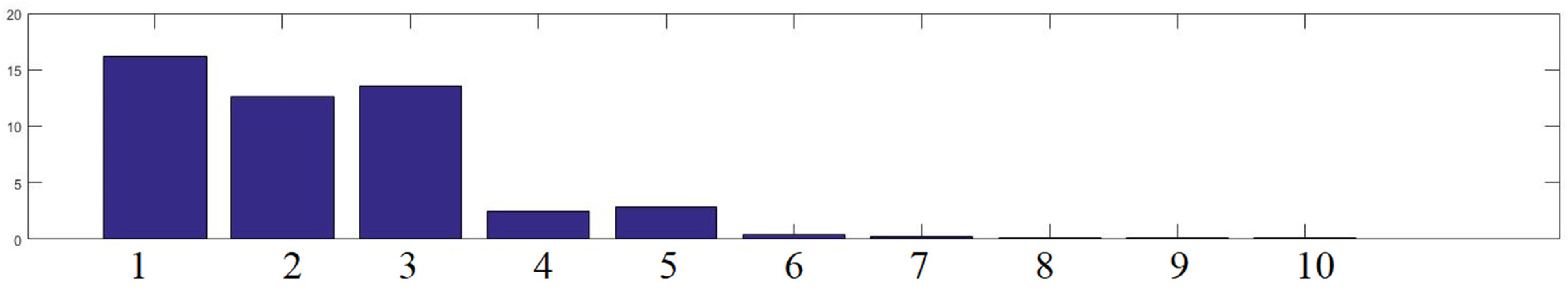
Figure 14.
Decomposition of the AE signal at eight levels using the proposed wavelet transform.
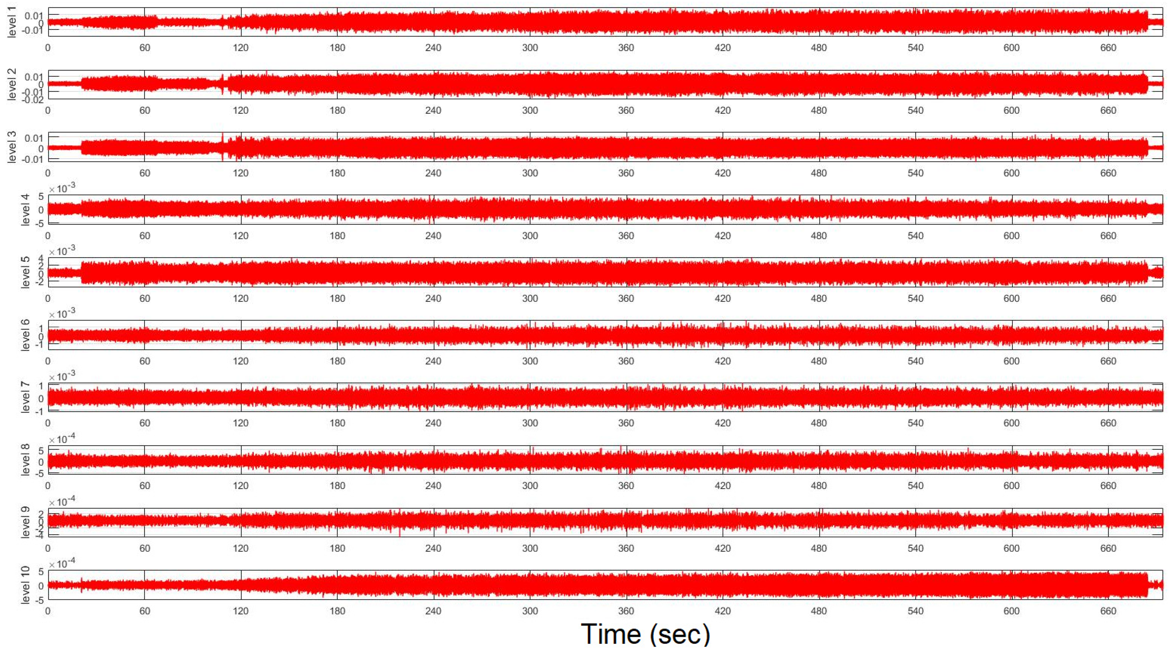
Figure 15.
Frequency response of the detail coefficients at 8 levels (1–8) for AE signal.
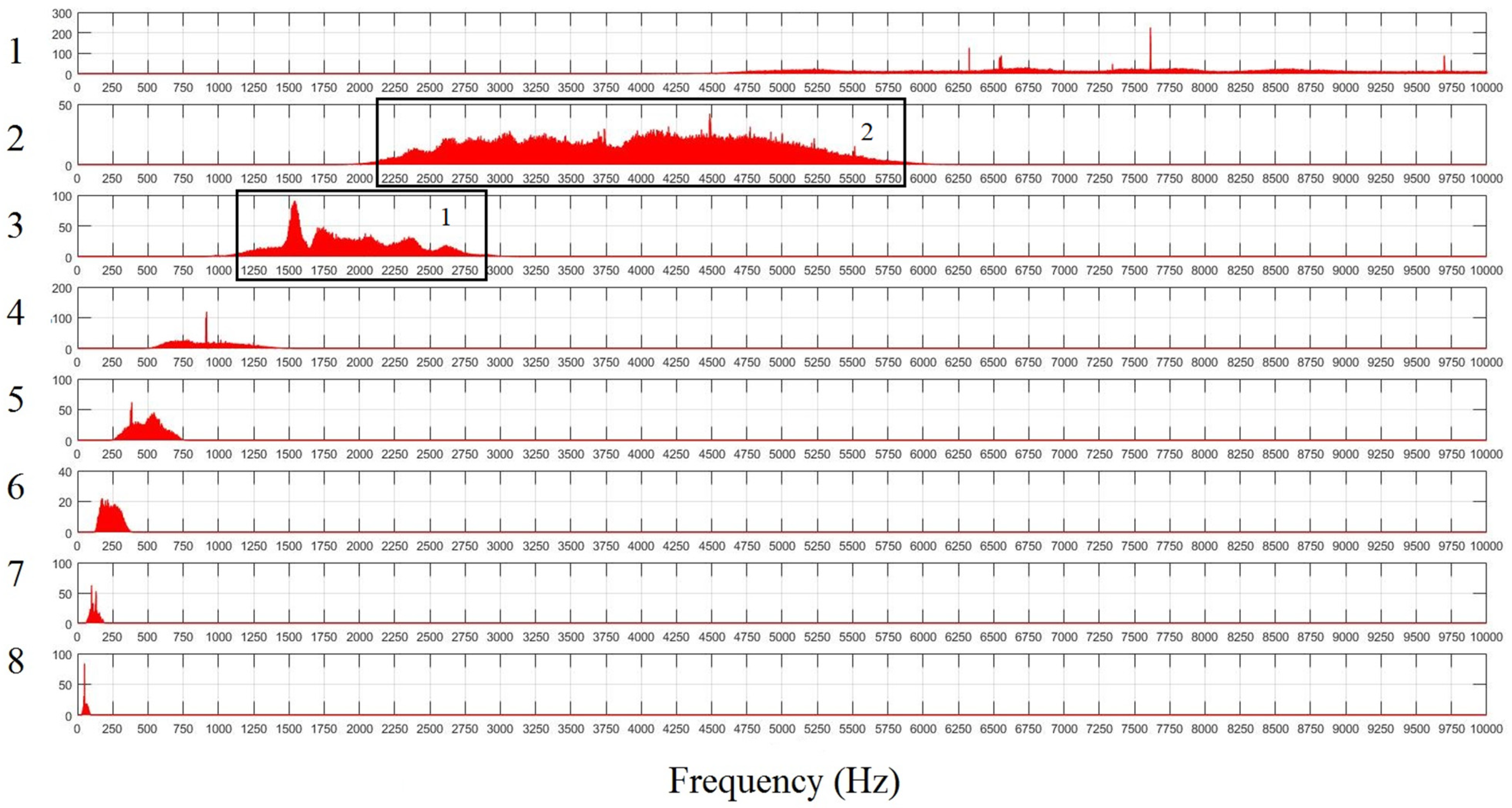
Figure 16.
Energy distribution of wavelet coefficients by decomposition levels during friction of ceramics based on Al2O3 and corresponding loads: (1) 20 N; (2) 30 N; (3) 45 N.
Figure 16.
Energy distribution of wavelet coefficients by decomposition levels during friction of ceramics based on Al2O3 and corresponding loads: (1) 20 N; (2) 30 N; (3) 45 N.

Figure 17.
Relative wavelet energy of wavelet coefficients corresponding to four wavelet levels decomposition (d1–d4).
Figure 17.
Relative wavelet energy of wavelet coefficients corresponding to four wavelet levels decomposition (d1–d4).

Figure 18.
(a) Total wavelet energy of wavelet coefficients vs. time in sec; (b) friction coefficient of alumina ceramics (Al2O3) against steel over time in sec.
Figure 18.
(a) Total wavelet energy of wavelet coefficients vs. time in sec; (b) friction coefficient of alumina ceramics (Al2O3) against steel over time in sec.
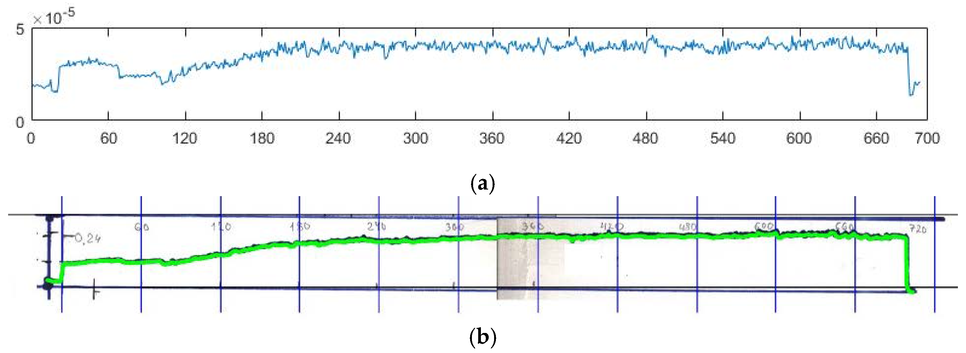
Figure 19.
(a) Total wavelet energy of the wavelet coefficients vs. time in sec; (b) total wavelet entropy of the wavelet coefficients vs. time in sec; (c) relative wavelet energy of wavelet coefficients for all levels of decomposition vs. time in sec.
Figure 19.
(a) Total wavelet energy of the wavelet coefficients vs. time in sec; (b) total wavelet entropy of the wavelet coefficients vs. time in sec; (c) relative wavelet energy of wavelet coefficients for all levels of decomposition vs. time in sec.

Figure 20.
Total wavelet entropy of the wavelet coefficients for three types of mother wavelets vs. time in sec.
Figure 20.
Total wavelet entropy of the wavelet coefficients for three types of mother wavelets vs. time in sec.
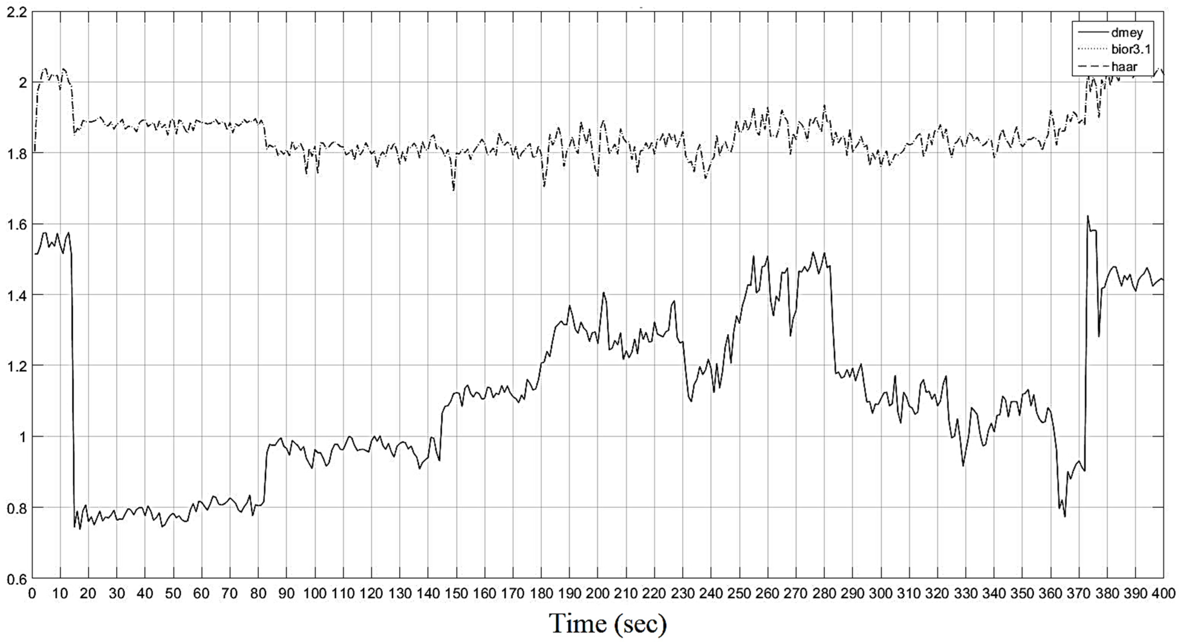
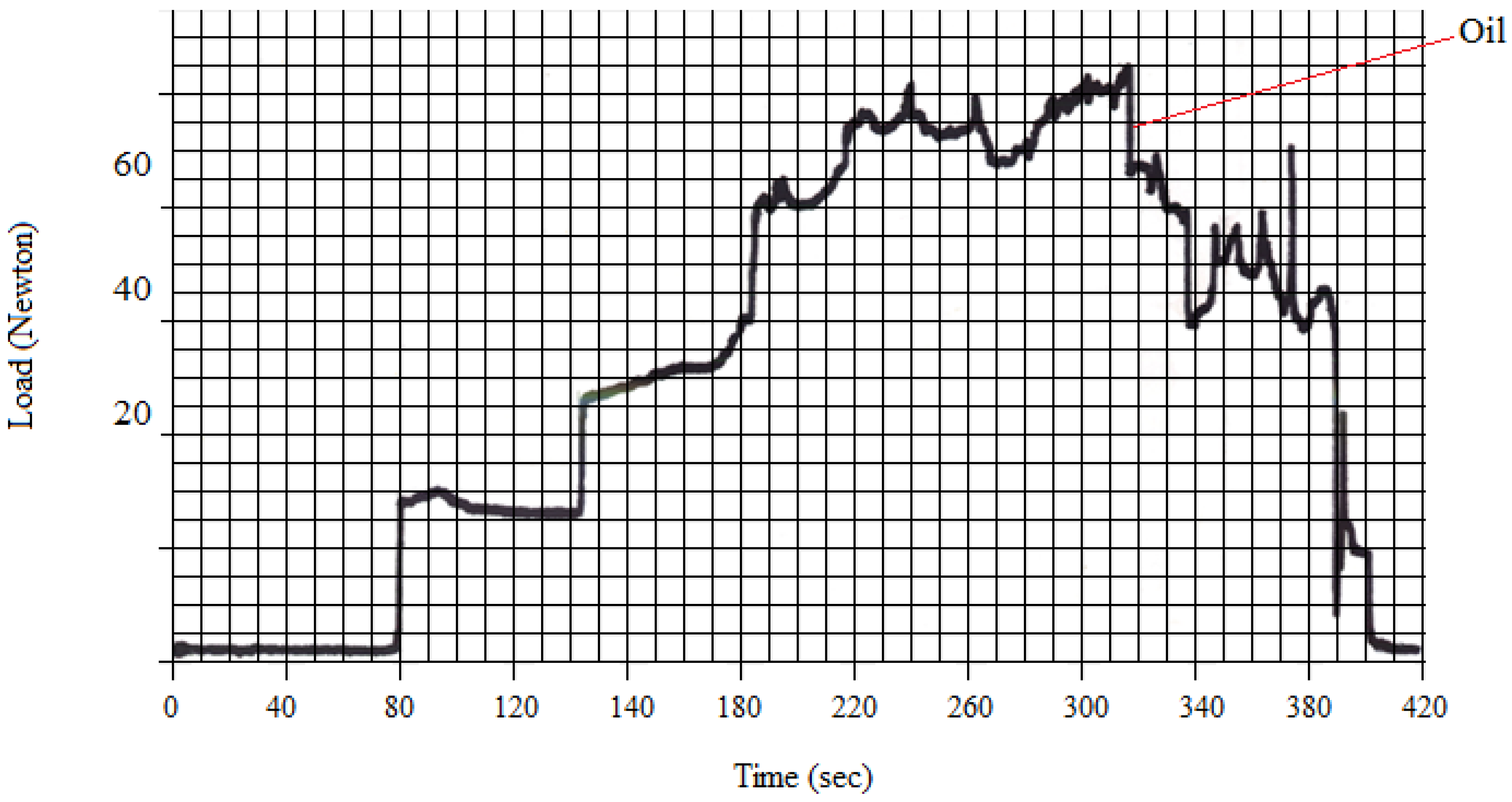
Figure 21.
Coefficient of friction aluminum against steel.


Table 1.
Frequency bands.
| Levels | Components | Frequency (Hz) |
|---|---|---|
| 1 | d1 | 5000–10,000 |
| 2 | d2 | 2500–5000 |
| 3 | d3 | 1250–2500 |
| 4 | d4 | 625–1250 |
| 5 | d5 | 312.5–625 |
| 6 | d6 | 156.25–312.5 |
| 7 | d7 | 78.125–156.25 |
| 8 | d8 | 39–78.125 |
| 9 | d9 | 19.53125–39.0625 |
| 10 | d10 | 9.765625–19.53125 |
Table 2.
Studied wavelet families.
| No | Mother Wavelet | No | Mother Wavelet | No | Mother Wavelet | No | Mother Wavelet |
|---|---|---|---|---|---|---|---|
| 1 | haar | 15 | sym5 | 29 | bior2.6 | 43 | rbio2.4 |
| 2 | db1 | 16 | sym6 | 30 | bior2.8 | 44 | rbio2.6 |
| 3 | db2 | 17 | sym7 | 31 | bior3.1 | 45 | rbio2.8 |
| 4 | db3 | 18 | sym8 | 32 | bior3.3 | 46 | rbio3.1 |
| 5 | db4 | 19 | coif1 | 33 | bior3.5 | 47 | rbio3.3 |
| 6 | db5 | 20 | coif2 | 34 | bior3.7 | 48 | rbio3.5 |
| 7 | db6 | 21 | coif3 | 35 | bior3.9 | 49 | rbio3.7 |
| 8 | db7 | 22 | coif4 | 36 | bior4.4 | 50 | rbio3.9 |
| 9 | db8 | 23 | coif5 | 37 | bior5.5 | 51 | rbio4.4 |
| 10 | db9 | 24 | bior1.1 | 38 | bior6.8 | 52 | rbio5.5 |
| 11 | db10 | 25 | bior1.3 | 39 | rbio1.1 | 53 | rbio6.8 |
| 12 | sym2 | 26 | bior1.5 | 40 | rbio1.3 | 54 | dmey |
| 13 | sym3 | 27 | bior2.2 | 41 | rbio1.5 | ||
| 14 | sym4 | 28 | bior2.4 | 42 | rbio2.2 |
Table 3.
Percentage of the energy distribution amongst decomposition levels.
| Level of Wavelet Decomposition | Frequency Range (Hz) | Percentage (%) |
|---|---|---|
| d1 | 5000–10.000 | 37.57 |
| d2 | 2500–5000 | 23.4 |
| d3 | 1250–2500 | 24.25 |
| d4 | 625–1250 | 6.8 |
| d5 | 312.5–625 | 5.87 |
| d6 | 156.25–312.5 | 1 |
| d7 | 78.125–156.25 | 0.86 |
| d8 | 39–78.125 | 0.24 |
Disclaimer/Publisher’s Note: The statements, opinions and data contained in all publications are solely those of the individual author(s) and contributor(s) and not of MDPI and/or the editor(s). MDPI and/or the editor(s) disclaim responsibility for any injury to people or property resulting from any ideas, methods, instructions or products referred to in the content. |
© 2024 by the authors. Licensee MDPI, Basel, Switzerland. This article is an open access article distributed under the terms and conditions of the Creative Commons Attribution (CC BY) license (https://creativecommons.org/licenses/by/4.0/).
Share and Cite
MDPI and ACS Style
Sychev, S.; Batako, A.D.L. A Study of Sliding Friction Using an Acoustic Emission and Wavelet-Based Energy Approach. Machines 2024, 12, 265. https://doi.org/10.3390/machines12040265
AMA Style
Sychev S, Batako ADL. A Study of Sliding Friction Using an Acoustic Emission and Wavelet-Based Energy Approach. Machines. 2024; 12(4):265. https://doi.org/10.3390/machines12040265
Chicago/Turabian StyleSychev, Sergey, and Andre D. L. Batako. 2024. "A Study of Sliding Friction Using an Acoustic Emission and Wavelet-Based Energy Approach" Machines 12, no. 4: 265. https://doi.org/10.3390/machines12040265
Note that from the first issue of 2016, this journal uses article numbers instead of page numbers. See further details here.