Article

An Intelligent Diagnostic Method for Wear Depth of Sliding Bearings Based on MGCNN

Department of Mechanical Engineering, Tsinghua University, Beijing 100084, China
*
Author to whom correspondence should be addressed.
Machines 2024, 12(4), 266; https://doi.org/10.3390/machines12040266
Submission received: 20 March 2024 / Revised: 13 April 2024 / Accepted: 14 April 2024 / Published: 16 April 2024

Abstract

:
Sliding bearings are vital components in modern industry, exerting a crucial influence on equipment performance, with wear being one of their primary failure modes. In addressing the issue of wear diagnosis in sliding bearings, this paper proposes an intelligent diagnostic method based on a multiscale gated convolutional neural network (MGCNN). The proposed method allows for the quantitative inference of the maximum wear depth (MWD) of sliding bearings based on online vibration signals. The constructed model adopts a dual-path parallel structure in both the time and frequency domains to process bearing vibration signals, ensuring the integrity of information transmission through residual network connections. In particular, a multiscale gated convolution (MGC) module is constructed, which utilizes convolutional network layers to extract features from sample sequences. This module incorporates multiple scale channels, including long-term, medium-term, and short-term cycles, to fully extract information from vibration signals. Furthermore, gated units are employed to adaptively assign weights to feature vectors, enabling control of information flow direction. Experimental results demonstrate that the proposed method outperforms the traditional CNN model and shallow machine learning model, offering promising support for equipment condition monitoring and predictive maintenance.

1. Introduction

Bearings are fundamental components of modern industry and are crucial for the development of a country’s heavy industry, earning them the nickname the “joints” of mechanical equipment. Their primary function is to support rotating mechanical bodies, reducing the coefficient of friction during their motion, and thus, they are widely applied in rotary machinery. Bearings can be roughly divided into two types based on their working principles: rolling bearings and sliding bearings. Among these, sliding bearings are mechanical elements that support rotating components using the principle of sliding friction and allow for relative sliding between the loading surfaces [1]. Their advantages include a compact structure, requiring minimal installation space, and high rotational accuracy. Moreover, since they do not rely on rolling, they experience less inertial force at high rotational speeds, resulting in smoother and more reliable operation with lower noise compared with rolling bearings [2]. This makes them indispensable in applications where high precision is required, radial dimensions are small, and lubrication is difficult to apply. As a result, sliding bearings are extensively used in aerospace, shipbuilding, automotive, high-speed railway transportation, precision machine tools, agricultural machinery, and other fields, becoming one of the core components of modern mechanical equipment [3].
As modern machinery evolves towards complexity, precision, and high-speed operation, the conditions under which bearings operate have become more demanding [4,5]. Due to relative sliding between the loading surfaces, bearings may experience wear and degradation under radial loading, potentially leading to excessive shaft eccentricity, fluid leaks, and interference between internal components [6]. Once a certain level of wear accumulates, it can result in the partial or complete loss of function of sliding bearings, affecting the safety and stability of the entire unit. For some heavy-duty equipment, the wear failure of sliding bearings can cause immeasurable economic losses and catastrophic events. Therefore, monitoring and predicting the wear state of sliding bearings during operation is of great significance [7].
There is currently a large amount of research on the state monitoring and prediction of components such as rolling bearings and machine tools, with numerous public datasets of mechanical product failures available worldwide for use [8,9,10]. Vencl et al. [11] systematically classified the wear failure of roller bearings, and established a fault tree for wear failure analysis. Li et al. [12] extracted a two-dimensional time–frequency image from the vibration signals of rolling bearings using a short-time Fourier transform and input it into a convolutional neural network for fault classification. Han et al. [13] proposed a rotary machinery fault diagnosis framework based on deep transfer learning. Wang et al. [14] used a relevance vector machine (RVM) to extract degradation features from the vibration signals of rolling bearings and fit an empirical exponential model to predict the remaining useful life (RUL) of rolling bearings. Zhu et al. [15] employed a superposed log-linear proportional intensity model to model and evaluate the reliability of incompletely maintained machine tools, quantitatively assessing the impact of maintenance activities on machine tool reliability. Wang et al. [16] conducted fault probability analysis on a disk-type tool magazine using Bayesian networks. SKF intelligent bearings are connected to external sensors to monitor and even control the entire operation of the bearings [17]. Alexander and Evgeny [18] studied the thermal analysis of bearing assemblies based on FEM and developed a methodological basis for implementing automatic diagnostics. Baron et al. [19] conducted diagnosis and analysis for bearings from the CNC machining center based on various vibrodiagnostic methods. In summary, existing intelligent diagnostic methods extract features from monitoring data and input them into classifiers or regressors for fault diagnosis or useful life prediction.
For sliding bearings, current research mainly focuses on issues such as rotor stability [20,21,22,23,24,25,26,27], calculation of oil film stiffness and damping [28,29,30,31], as well as material wear resistance performance [32,33,34], aiming to enhance the lubrication performance and wear resistance of bearings at the design stage. Although improving the lubrication performance and wear resistance of sliding bearings can effectively alleviate material wear problems, wear is inevitable during equipment startup, shutdown stages, and under the influence of some unexpected factors [35]. Some scholars use numerical models to simulate and predict the wear behavior of bearings. Jeon et al. [36] used a typical journal wear test to statically predict the wear of the joint bearing. König et al. [37] predicted the macroscopic wear amount of sliding bearings based on the Archard model and Fleischer model. Dai and Tian [38] introduced a sequential hybrid model of neural network and finite element for predicting wear in sliding bearings. In general, these methods simulate and predict bearing wear based on static conditions and cannot integrate with online data. Therefore, implementing real-time diagnosis and quantitative evaluation of the wear state during the operation of sliding bearings, and subsequently performing predictive maintenance, is of significant importance for enhancing equipment safety and reducing maintenance costs.
From a structural standpoint, sliding bearings and rolling bearings exhibit significant differences. The latter typically consists of components such as inner and outer rings, cages, and rollers, making their structure comparatively complex [39], while sliding bearings are characterized by a simpler structure, usually comprising a shaft journal and bearing, sometimes with coatings in certain scenarios. This disparity results in the vibration signals during the degradation process of sliding bearings being less pronounced compared with rolling bearings. Consequently, the data characteristics of status detection signals differ considerably between the two types of bearings. Currently, there is a scarcity of online diagnostic methods specifically tailored to sliding bearings, and there is also a lack of widely accepted data concerning the failure lifecycle of sliding bearings. Therefore, focusing on the diagnosis and prognosis of sliding bearings, it is still necessary to conduct experiments on and analyses of monitoring data to develop practical and feasible wear diagnostic methods.
Since the maximum wear depth (MWD) of a sliding bearing is equivalent to the clearance of a shaft bearing, this paper uses MWD as a quantitative indicator for assessing the bearing’s wear condition and proposes an intelligent diagnostic method based on a multiscale gated convolutional neural network (MGCNN), which can be trained and inferred based on online vibration signals of bearings and can quantitatively evaluate the MWD of bearings to characterize their current wear state. The contributions of this work are summarized as follows:
  • Different from the current research focus on the lubrication and antiwear performance of sliding bearings, this paper aims to dynamically diagnose and quantitatively evaluate the wear state during the operation of bearings. In typical situations, MWD directly impacts bearing performance, yet is often challenging to measure directly in real time. Conversely, vibration signals can be continuously collected through external sensors. Leveraging the vibration signals collected during the operation of sliding bearings, this paper proposes an end-to-end approach to infer the MWD affecting bearing performance, enabling the diagnosis of bearing conditions. This bridges a gap in the current research landscape of sliding bearings by providing an intelligent diagnostic method.
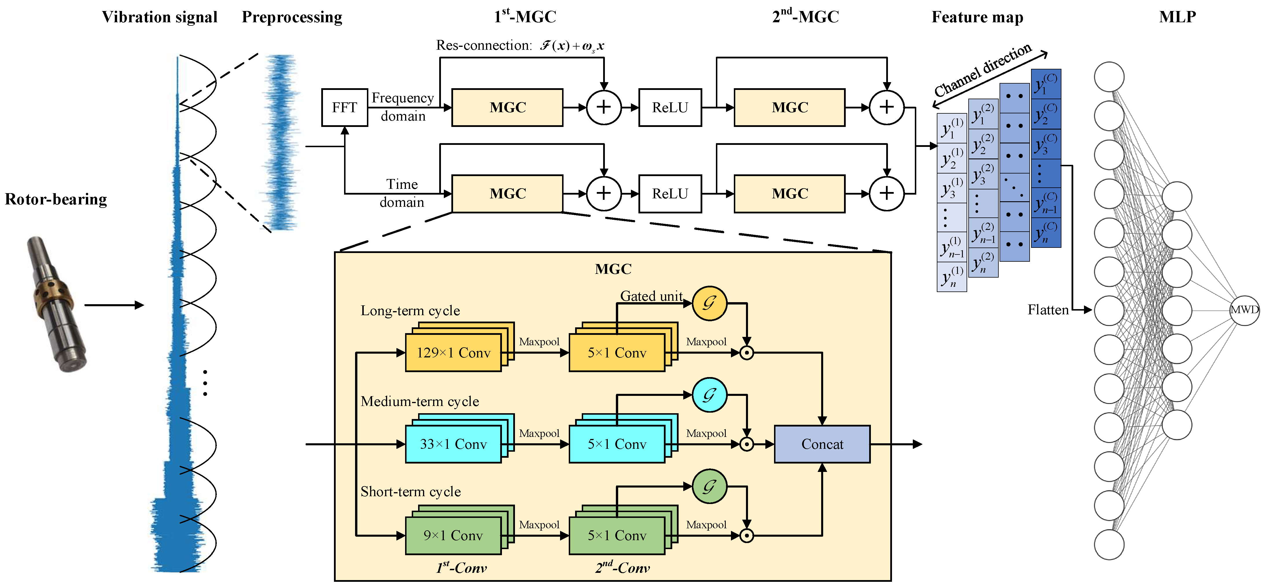
  • An MGCNN intelligent diagnostic model is constructed, with vibration signals as input and the bearing’s MWD as output. Considering the periodic characteristics of rotating machinery, the established MGCNN model adopts a dual-path parallel structure in both time-domain and frequency-domain to fully extract valid information from bearing vibration signals, thereby enhancing the model’s prior knowledge. The MGC module is designed, which utilizes three channels for long-term, medium-term, and short-term cycles to extract multiscale information from vibration signals; meanwhile, gated units are designed to assign weights to feature vectors through nonlinear mappings. By amplifying the weights of important features and disregarding unimportant ones, the control of information flow is achieved.
  • Building upon the diagnostic results of the proposed method, this paper further conducts predictive maintenance for sliding bearings. By setting a predefined wear threshold, this paper determines a bearing’s remaining useful life, facilitating predictive maintenance for bearings and equipment.
The remainder of this paper is organized as follows. Section 2 describes the bearing wear problem and introduces the related deep learning theories and foundations; Section 3 introduces the proposed MGCNN model; Section 4 presents the bearing wear test and validates, analyzes, and discusses the proposed model; Section 5 provides the conclusions of this work and discussions on future work.

2. Bearing Vibration Signals and Deep Neural Networks

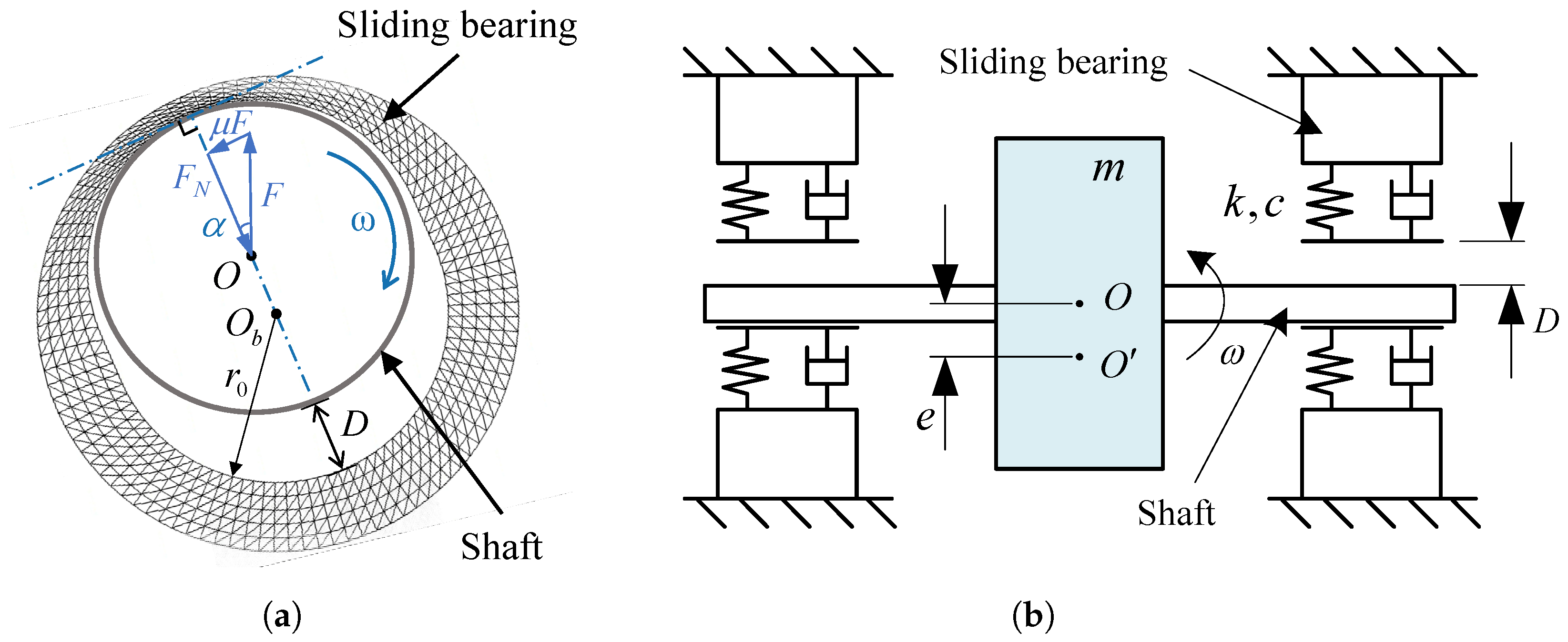
2.1. Wear State and Diagnosis of Sliding Bearing

As shown in Figure 1a, the common assembly form of sliding bearings is the rotor–bearing fit, where the rotor rotates under the support of sliding bearings. The surface of the shaft contacts and slides relative to the inner surface of the bearing. Since the rotor is often subjected to a radial load F and shaft rotation, the inner surface of the bearing is prone to wear in a fixed direction. The wear of the bearing’s inner surface results in an abnormal clearance D between the shaft and the bearing. As shown in Figure 1b, the rotor is considered as an eccentric mass block and the sliding bearing as a spring-damping support, and the abnormal clearance caused by bearing wear leads to abnormal vibration during rotor rotation. Moreover, the vibration signal is directly related to the size of the clearance D. It is worth noting that because the bearing load-bearing surface is an arc, the wear depth at each node is not uniform, and the clearance D is equal to the maximum wear depth (MWD). In actual systems, vibration signals can be collected by deploying sensors on the equipment surface, while the bearing wear depth is difficult to measure online. Therefore, this paper focuses on the research of sliding bearing wear diagnosis, establishes an intelligent diagnostic model, and infers the current maximum wear depth of the bearing based on the vibration signals collected from the worn sliding bearing.

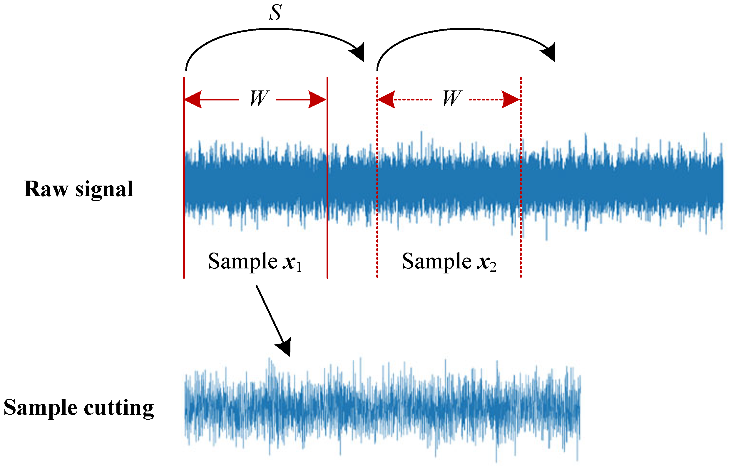
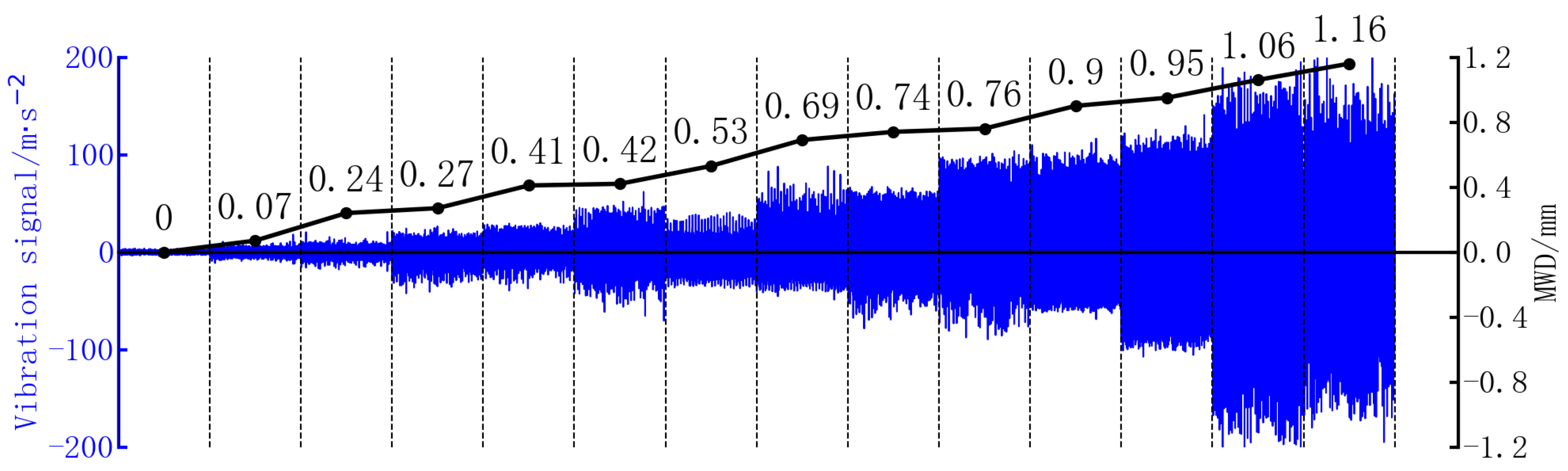
2.2. Sample Cutting and Preprocessing

When the vibration signal x of a bearing is collected over a period of time, data preprocessing is performed first, as shown in Figure 2. The purpose of data augmentation is to increase the diversity of the dataset [40], allowing the model to better learn the various variations and complexities of the data during training, thereby enhancing the model’s generalization ability and robustness.
In practical applications, data augmentation is commonly regarded as an effective strategy to improve the performance of deep learning models. For the original vibration signal x t = [ x 1 x 2 x L ] , specifying a sample length W and a stride S, we obtain several shorter samples x 1 , x 2 , ⋯, x n by slicing the raw signal. By reducing the sample length and increasing the number of samples, we provide more comprehensive training for the neural network, where the number of samples is n = mod ( l e n ( x ) L , S ) , and mod ( · ) represents the modulo operator. The obtained new samples are as follows:
x i = x 1 + ( i 1 ) S x 2 + ( i 1 ) S x W + ( i 1 ) S
Additionally, this paper involves the deliberate addition of noise to the raw data, enabling the model to learn features that more accurately represent bearing degradation information. Related experiments and discussions are conducted in Section 4.4. The process of adding noise is as follows:
x i ^ = x i + ϵ
where x i is the raw sample, and ϵ is the noise. This paper employs Gaussian white noise ϵ N ( 0 , σ 2 ) , where ϵ follows a normal distribution with a mean of 0 and a variance of σ 2 . The hyperparameter σ determines the intensity of the noise.
It is worth mentioning that in time series analysis problems, multiscale entropy (MSE) is commonly used to quantify the complexity of time series [41]. Ref. [42] explored the linear correlation between multiscale permutation entropy (MPE) and multiscale weighted permutation entropy (MWPE) using the slope of linear regression as a discriminant statistic. Building on this, Ref. [43] investigated the effects of the optimal parameters of nonuniform embedding. In this paper, the diagnostic task is abstracted as a regression problem rather than a pure time series prediction problem, meaning it focuses on outputting evaluation metrics based on input vectors. Therefore, the current work does not delve deeply into the complexity of vibration signal time series. Integrating time series analysis techniques will be a potential research point in future work.

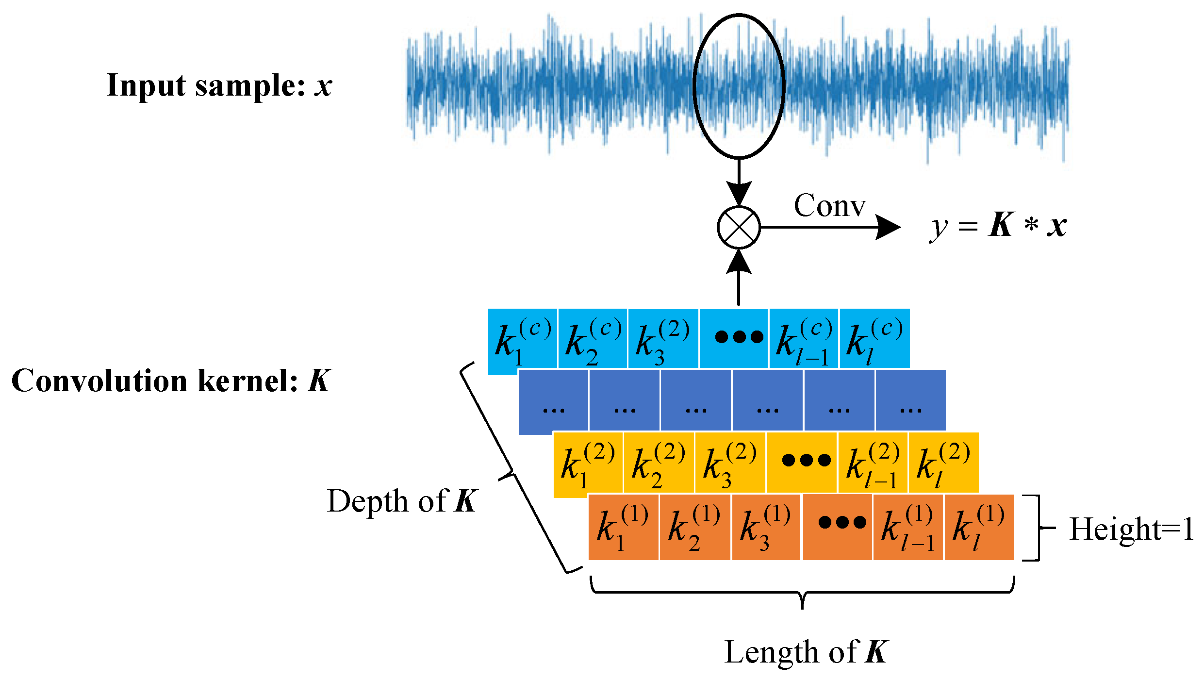
2.3. Convolutional Neural Network

After obtaining samples through data preprocessing, this paper uses convolutional neural network layers to extract features from sample sequences, where convolutional kernels are used to perform convolution operations on local regions of the input signal [44], obtaining the corresponding features, as shown in Figure 3. For bearing condition data, taking vibration signals as an example, they are one-dimensional vectors containing several elements. The weight sharing in the convolutional layer allows a single convolutional kernel to traverse the entire input vector, effectively reducing the scale of network parameters. Generally, the size of a convolutional kernel is the depth c conv ∗ width l conv ∗ height h conv , where the depth is consistent with the number of channels of the input data; for one-dimensional vibration signals, the height h conv is 1, so the size is c conv × l conv . Therefore, a convolutional kernel can be represented as follows:
K = k 1 ( 1 ) k 2 ( 1 ) k l ( 1 ) k 1 ( 2 ) k 2 ( 2 ) k l ( 2 ) k 1 ( c ) k 2 ( c ) k l ( c )
Using the convolutional kernel K to perform a sliding convolution over the sequence samples, the feature y obtained from a single channel in a single convolution is as follows [44]:
y i = m = 1 c n = 1 l k n ( m ) x n ( m )
where x n ( m ) is the nth element of the mth channel in the current convolutional region.
After convolution, the samples typically undergo pooling processing, which serves to suppress noise, reduce computational complexity, and prevent overfitting, among other functions. Common pooling operations include max pooling and average pooling, which use the mean and maximum values within the pooling filter region as the pooling output, respectively. Due to the symmetry typically found in vibration signals in the time domain, using average pooling might result in features close to zero after pooling, leading to ineffective features. Therefore, this paper employs max pooling [44], which is defined as follows:
y i j = max x k R i j x k
where R i j represents the region of influence of the pooling filter. Figure 4 illustrates the max pooling process for one-dimensional samples, with a pooling filter size of 2 × 1 and a stride of 2.
After the samples have undergone convolution or pooling, an activation function is applied to the convolutional output to perform a nonlinear transformation. According to reference [45], commonly used activation functions include the Sigmoid function (Equation (6)), the Tanh function (Equation (7)), and the ReLU function (Equation (8)):
f Sigmoid ( y ) = 1 1 + e y
f Tan h ( y ) = e y e y e y + e y
f ReLU ( y ) = max ( y , 0 )
The curves corresponding to the three activation functions are shown in Figure 5. Due to the fact that deep neural networks update network weights through the backpropagation algorithm by transferring gradients layer by layer, for the Sigmoid and Tanh functions, when the absolute value of the input is large, the curve will saturate, and the gradient will approach 0. As the number of layers in the neural network increases, these smaller gradients will gradually propagate through each layer, eventually leading to slow or stagnant parameter updates in the deep network. This prevents the network from fully learning complex features, thus affecting the convergence and output performance of the model, a phenomenon known as gradient vanishing [46,47]. Therefore, this paper adopts the ReLU activation function, which has a gradient of 1 for positive inputs, helping to alleviate the gradient vanishing problem and allowing the proposed neural network structure to be trained more effectively.

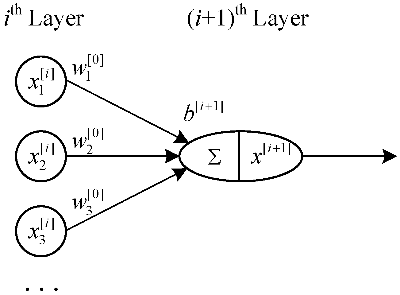
2.4. Fully Connected Neural Network

The Universal Approximation Theorem [48,49] states that a feedforward neural network with a linear output layer and at least one hidden layer with any kind of “squashing” activation function can approximate any Borel measurable function from one finite-dimensional space to another with arbitrary precision, provided that the network has enough hidden units. Therefore, this paper selects the fully connected neural network as the output module of the proposed method model, also named Multilayer Perceptron (MLP).
The basic structure of a fully connected neural network is shown in Figure 6, where each neuron in the i th layer is connected to every neuron in the ( i + 1 ) th layer. The mathematical expression for this is [45]
x [ i + 1 ] = f act ( j w j [ i ] x j [ i ] + b [ i + 1 ] )
where f act is a nonlinear activation function. If no activation function is added, the fully connected neural network can only express linear models. Here, the ReLU function shown in Equation (8) is also adopted.
In terms of model training, neural networks use the error backpropagation algorithm to calculate the derivatives of the loss function concerning the model parameters and update the parameters to minimize the loss function. For cases where the dataset is small or the model parameter space is limited, Stochastic Gradient Descent (SGD) [50] can converge to the global optimum. However, in high-dimensional parameter spaces and with complex loss functions, the Adam optimizer (Adaptive Moment Estimation) [51] often requires fewer hyperparameter adjustments and exhibits better convergence performance. Considering the multimodule coupling of the proposed intelligent diagnostic method and the complexity of the network units, this paper uses the Adam method to optimize the established deep learning model, as shown in Algorithm 1.
Algorithm 1 Adam [51]
Require: 
Stepsize: α ; exponential decay rates for the moment estimates: β 1 , β 2 [ 0 , 1 ) ; constant ϵ = 10 8 ; model parameters: θ ;
 
    Initialize 1st moment vector: m 0 = 0 ; 2nd moment vector: v 0 = 0 , and timestep: t = 0
Ensure: 
Optimised parameters: θ t
  1:
while  θ t not converged do
  2:
    t t + 1
  3:
    g t θ L ( θ t 1 ) , where L ( θ ) is the objective function with parameters θ
  4:
    m t β 1 · m t 1 + ( 1 β 1 ) · g t
  5:
    v t β 2 · v t 1 + ( 1 β 2 ) · g t g t , where⊙ represents element-wise multiplication of vectors.
  6:
    m ^ t m t / ( 1 β 1 t )
  7:
    v ^ t v t / ( 1 β 2 t )
  8:
    θ t θ t 1 α · θ t / ( v ^ t + ϵ )
  9:
end while

3. Multiscale Gated Convolutional Neural Network

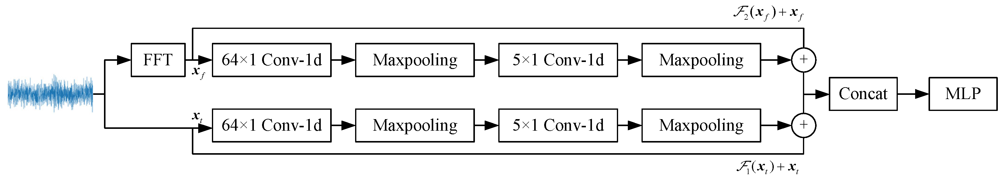
3.1. Overall Structure of the MGCNN

The proposed method for sliding bearing wear diagnosis based on the multiscale gated convolutional neural network (MGCNN) is shown in Figure 7. The original vibration signals are subjected to data augmentation, and after sample cutting, they are input into MGCNN for feature extraction and regression fitting. Due to the rotational periodicity of rotating machinery, the vibration signals also contain rich degradation fault information in the frequency domain. Therefore, in addition to directly extracting features from the time-domain signals, a Fourier transform [52] is applied to the time-domain signals to obtain the frequency-domain signals:
x f , j = k = 1 m x t , k e i 2 π m j ( k 1 ) , k = 1 , 2 , m
Features are extracted from the frequency-domain signals using neural networks to capture the frequency-domain information. Consequently, the structure of the training data is { ( x t , x f ) , D label } , where D label represents the true value of maximum wear depth, which is the data label.
The MGCNN includes time-domain and frequency-domain pathways, each with two levels of multiscale gated convolution (MGC) modules to extract features from their respective domains. The feature maps obtained from the MGC modules are concatenated along the channel direction, and the output of the 1 st -MGC passes through a ReLU activation function before entering the 2 nd -MGC. Since the original vibration signal is a one-dimensional vector, the input channel number for the 1 st -MGC module is 1, while the input channel number for the 2 nd -MGC module equals the output channel number of 1 st -MGC. Every time the data pass through an MGC, the feature length is reduced to 1/8 of its original size. Since the signal undergoes a Fourier transformation at the outset on the frequency domain path, the feature length is always half that of the corresponding position on the time–frequency path. Finally, the feature maps are flattened and input into the MLP for regression fitting to obtain the maximum wear depth.
In theory, if a neural network with fewer layers has already achieved a high level of accuracy, then adding more layers should result in a network that is at least as accurate as the original. This is because, if the added layers are identity transformations, the output accuracy of the network before and after the addition should be the same; moreover, the additional layers should, in principle, be trainable to perform even better. However, in practice, deep neural networks exhibit a phenomenon known as “degradation”, where, as the network depth increases beyond a certain point, the model’s accuracy unexpectedly and significantly decreases [53].
A qualitative analysis of the reasons behind this phenomenon reveals significant differences between deep learning and traditional machine learning, particularly in terms of deeper network structures, the application of nonlinear activation functions, and the automated process of feature extraction and transformation. In deep learning, the introduction of nonlinear activation functions is crucial as it allows data to be mapped into higher-dimensional spaces, facilitating better classification and regression. However, as the number of network layers increases, so does the number of introduced nonlinear activation functions, leading to the mapping of data into more complex nonlinear spaces. Due to the complexity of this mapping, it becomes very difficult to restore the data to their original space (i.e., to perform an identity transformation). In other words, the neural network requires a considerable amount of computation to remap the data back to their original space, which may exceed the computational capabilities supported by the current data and hardware resources.
To address this issue, the MGCNN adopts a residual neural network structure [54]. In the constructed neural network model, residual connections are placed at both ends of each MGC module to ensure the integrity of data information transmission. By introducing residual connections between the input and output of the neural layers, the output of the neural layer is no longer a direct feature mapping but a residual of the input, i.e., the difference between the layer’s input and output. This type of connection allows the network to more easily learn identity mappings, thereby simplifying the optimization of deep networks. For a stacked-layer neural network, the output of layer l is x l = F ( x l 1 ) ; however, the output of a residual unit is
x l = F ( x l 1 ) + ω s x l 1
where ω s represents the transformation parameters to maintain the same shape between ω s x l 1 and F ( x l 1 ) ; specifically, in this paper, ω s is achieved using 1 × 1 convolutional kernels with certain strides. This allows the stacked layer to act as an identity transformation when F ( x l 1 ) = 0 , ensuring that the network’s performance does not decrease with the addition of this stacking layer.
In this paper, the Dropout technique is used in MLP to improve the model’s generalization ability [55]. During the network training process, Dropout randomly sets the output of neurons to zero with a certain probability to prevent certain parts of the network from being overly dependent on specific samples. This reduces the coupling between neurons in the neural network, making the network sparser and thereby reducing overfitting.

3.2. Structure of the MGC Module

To fully extract the multiscale periodic information from bearing vibration signals, the MGC module sets up three channels in parallel: a long-term cycle, a medium-term cycle, and a short-term cycle. These channels achieve multiscale periodic feature extraction through convolutional kernels of different lengths. For machine learning models, more complex models often have stronger feature representation capabilities. Traditional stacked networks mainly increase model complexity by stacking network layers, which simultaneously brings about the issues of vanishing/gradients explosion; whereas the parallel convolutional layer structure increases the “width” of the network rather than its “depth”, enhancing the model’s capability to represent complex features while somewhat mitigating the vanishing/gradients explosion phenomena [56]. In the MGC module, after the first convolution operation is completed, max pooling is applied, followed by a further feature abstraction using a small convolution kernel, and then pooling again. Each scale channel has a gated unit G ( · ) , and the output after the gated unit is as follows:
y = x G ( x )
where x is the output after convolution and max pooling, serving as the input to the gated unit; G ( · ) is the gating function that maps x to the interval (0, 1); and the ⊙ operator denotes element-wise multiplication of vectors/matrices of the same size, as shown in Figure 8.
In this paper, the gated unit uses a Sigmoid function (as shown in Equation (6)), so the gating mapping relationship is fixed and does not change with the model. The following represents the feature maps processed by the gated unit in matrix form:
Y = G ( x 1 ( 1 ) ) x 1 ( 1 ) G ( x 2 ( 1 ) ) x 2 ( 1 ) G ( x m ( 1 ) ) x m ( 1 ) G ( x 1 ( 2 ) ) x 1 ( 2 ) G ( x 2 ( 2 ) ) x 2 ( 2 ) G ( x m ( 2 ) ) x m ( 2 ) G ( x 1 ( c ) ) x 1 ( c ) G ( x 2 ( c ) ) x 2 ( c ) G ( x m ( c ) ) x m ( c )
where x i j represents the features after convolution mapping, and G ( x i j ) is the weight value of after being processed by the gated unit, so G ( x i j ) · x i j forms the final features, making up the feature map Y . Each element in matrix Y represents a feature in a certain dimension, but not all features reflect information about bearing wear and degradation. Qualitatively, the feature map Y is divided into two parts:
Y = G ( x + ) x + + G ( x ) x
where x + represents features related to degradation information, while x represents irrelevant features. Because x does not provide effective features and may even interfere with the model’s judgment, we assign smaller weights to these features through the gated unit to minimize their impact on the model’s regression inference. The specific process is achieved through the optimization of model parameters. It is worth mentioning that since this paper uses the Sigmoid function as the gated unit, which is a fixed function, the weights assigned to x by the gating unit are actually determined by x itself. We know that x is the feature obtained from convolution. Therefore, from the perspective of model training, the gated unit affects the optimization of convolution kernel parameters, effectively adding a prior constraint to the optimization process that makes it easier for parameters to converge to the global optimum. Additionally, the gated unit could be set as an independent function, also based on training sets for parameter optimization, but this approach would place further demands on the scale and quality of the dataset, which we do not discuss further here.
Equation (14) shows that by introducing a nonlinear function G to map the output of the current layer and multiplying it with the original output as a weight, the adaptive enhancement of the importance of important information and the ignoring of unimportant information are achieved, thereby regulating the flow of information and serving as a “gate”. This operation based on the gated unit has several advantages. Firstly, the introduction of the gated unit allows the neural network to adaptively regulate the importance of each feature in the information transmission. In traditional neural networks, all features are treated equally, whereas the gated unit, through learning weight adjustments, allows the network to handle the contributions of different features to the task more flexibly. This mechanism is similar to the processing of information in the human brain and can better simulate human cognitive processes, thereby enhancing the representation and generalization capabilities of the neural network. Secondly, the gated unit can help the neural network better deal with noise and redundant information in the data. Due to external interference and factors such as assembly clearance, bearing vibration signals often contain a large amount of irrelevant information. The gated unit can adjust weights to selectively transmit features meaningful to the task and suppress the transmission of useless information, thereby improving the robustness and anti-interference ability of the model. Additionally, the gated unit can mitigate issues such as gradient disappearance and gradient explosion to some extent. By introducing a nonlinear function, the gated unit can effectively clip and adjust gradients, avoiding excessive growth or disappearance of gradients during backpropagation, which is conducive to accelerating the convergence speed of the network and improving training efficiency and stability. Therefore, the introduction of the gated unit provides a flexible and efficient information processing method for the network, which helps to enhance the performance and application scope of the model.
It is worth noting that Equation (3) shows that the one-dimensional convolution kernel has a depth direction, equal to the number of channels of the input sample. In the two levels of MGC modules in the constructed network structure, the input to the first-level MGC is the time–frequency domain vibration signal with one channel; the input to the second-level MGC is the output of the first-level MGC, and the number of channels at this point is a predefined hyperparameter, determined by the network structure. The multiscale convolution kernels are set with a stride of 1, and to maintain the same feature length before and after convolution, the zero-padding length is designed according to the following rules:
N padding = l conv 1 2
where l conv is the length of the convolution kernel, and · denotes the floor function.

3.3. Detailed Model Parameters

The detailed parameters of the designed network model are shown in Table 1. The number of zero-padding in the convolution and pooling layers is calculated according to Equation (15), which is not given in the table. The depth of the convolution kernel is equal to the number of input channels.

4. Experiment and Discussion

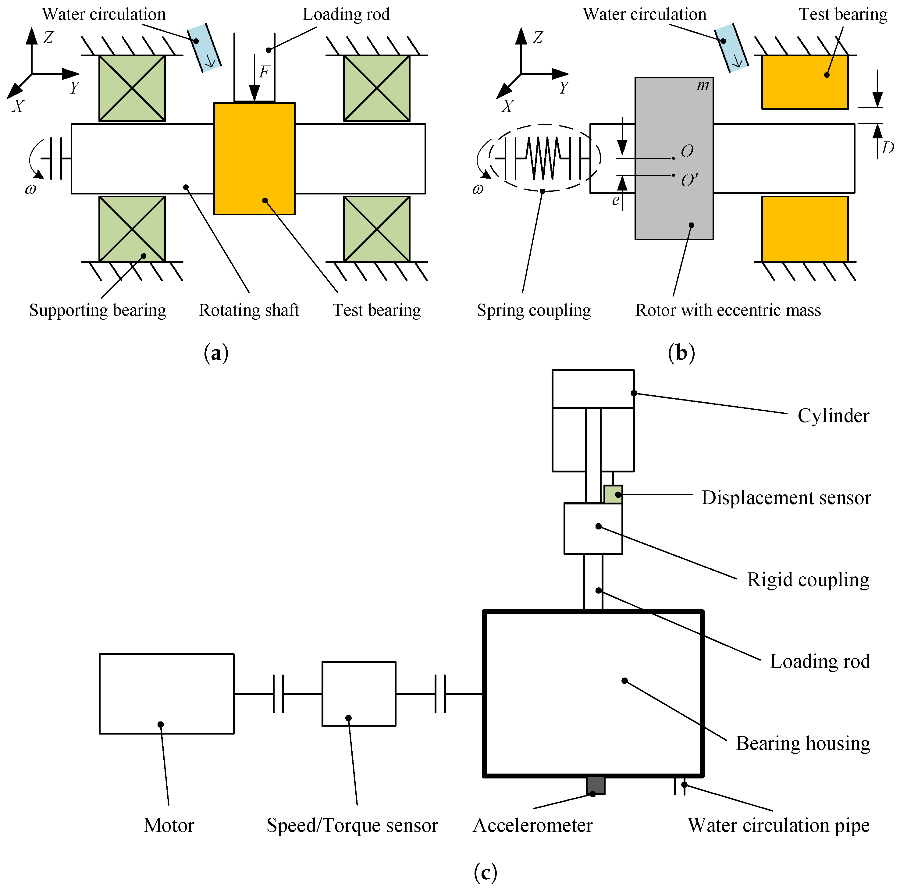
4.1. Wear and Vibration Test of Sliding Bearings

It should be noted that the experiments and validations in this paper consider vibrations originating solely from bearings, without interference from degradation of other components. When lubrication is insufficient in sliding bearings, wear behavior is prone to occur on the load-bearing surface, and a certain degree of wear depth can accumulate, leading to excessive clearance between the journal and the bearing, which in turn causes abnormal vibration of the rotor. To quantitatively study the relationship between the vibration signals under bearing wear conditions and the depth of bearing wear, a sliding bearing wear test platform was designed and set up in our related work [57]. The wear test is divided into two parts:
  • During the sliding bearing wear test stage, the inner surface of the bearing contacts the middle section of the shaft, and the bearing remains stationary in the circumferential direction while being subjected to a fixed direction and amplitude load radially. The two ends of the shaft are supported by cylindrical roller bearings, which are constrained axially and radially, and maintain a constant speed rotation in the circumferential direction, as shown in Figure 9a. In this stage, the test bearing transitions from a healthy state to a worn state.
  • In the vibration measurement stage of the worn bearing, the worn test bearing is fixed in a bearing housing as a support for one end of the shaft, while the other end of the shaft is connected to an electric motor through a spring coupling. An eccentric mass block m is attached to the shaft, with an eccentricity e, and the shaft rotates at a constant speed in the circumferential direction. As shown in Figure 9b, D is the clearance between the journal and the bearing, which is also the maximum wear depth of the bearing.
The established sliding bearing wear test platform is shown in Figure 10. A self-lubricating brass bushing with graphite was used as the test bearing, and the shaft material was a modulated steel. A cylinder, through a loading rod, applies a radial load on the surface of the test bearing, and a displacement sensor measures the displacement of the loading rod, which is used to characterize the bearing wear depth during the test process. A single-axis accelerometer was deployed on the surface of the bearing housing to collect bearing vibration signals. Additionally, the test platform collects motor torque and bearing surface temperature. A worn bearing is shown in Figure 11.
According to various scenarios, sliding bearings operate at specific rotational speeds, ranging from several hundred to several thousand revolutions per minute. In our experiments, the motor speed was set to 3500 r/min, which is a relatively common moderate speed. Multiple test specimens were used for wear tests of different durations to obtain several sliding bearings with different wear depths, and vibration tests were conducted. The vibration signals under different wear depths are shown in Figure 12, and the wear depths ( μ m ) included are as follows:
D label = [ 0 , 70 , 240 , 270 , 410 , 420 , 530 , 690 , 740 , 760 , 900 , 950 , 1060 , 1160 ]
It is worth mentioning that in the experiment, each wear depth value was actually sampled for several segments, and Figure 12 only shows the vibration signals of 1 s in length corresponding to each wear depth.

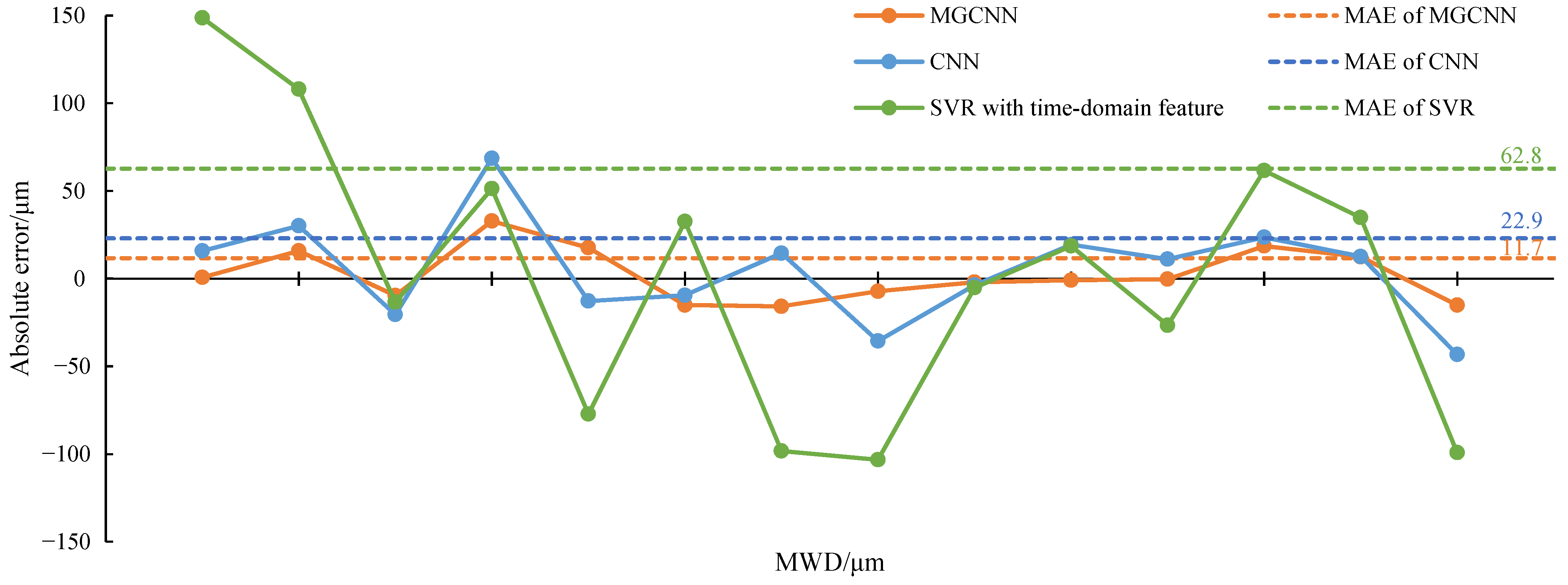
4.2. Wear Depth Diagnosis

The set sample length W = 2048 , and the stride S = 512 . Data augmentation is applied to the samples with overlapping cuts. The original sample length is 25,600, with a quantity of 621. After cutting, the number of samples increases to 29,187, with each sample now having a length of 2048.
The mean squared error (MSE) is used as the loss function:
e MSE = 1 N i = 1 N ( D ^ i D label , i ) 2
where D ^ i represents the output of the model, and D label , i is the true value.
The set batch size n batch = 512 , the learning rate α = 5 × 10 4 , and the number of training epochs n epoch = 50 . There are 14 different wear depths, which correspond to 14 classes of labels, and each label has several samples. Since the samples are generated from the original data through overlapping cutting, to avoid data leakage between the test set and the training set, the first 100 samples from each label are taken as the test set, and the remaining data are used for training and validation. This means that at most 3 samples in each label’s 100 test samples may overlap with the training data, which is negligible. The test set contains a total of 1400 samples. The remaining 27,787 samples are divided into the training set and the validation set according to k-fold cross-validation method ( k = 5 ).
As shown in the validation loss function curve of the training process in Figure 13, it can be seen that the model’s loss function on the validation set exhibits a stable downward trend as training progresses, and it can reach a stable convergence state around epoch n epoch = 15 .
As described, the method undergoes 5 rounds of training, and the best model on the validation set for each round is used for testing. The average output of the 5 models on the test set is taken as the final result. This paper compares the proposed method with traditional diagnostic methods, including a single-scale CNN network, as illustrated in Figure 14, and a shallow machine learning model, support vector regression (SVR), which extracts 11 time-domain features and 12 frequency-domain features referring to reference [58]. It should be noted that since the SVR training process does not involve batching and random reading of samples, and k-fold cross-validation was not adopted.
The wear diagnosis results of the models are shown in Table 2. It is worth mentioning that the SVR diagnostic error using time–frequency domain features is too large, so an SVR model using only time–frequency features was added as a control. To evaluate the performance of the models on the entire test set, the mean absolute error (MAE) was calculated by taking the absolute value mean of the test errors under each label. The calculation results are MAE MGCNN = 11.7 , MAE CNN = 22.9 , MAE SVR - 1 = 287.1 , and MAE SVR - 2 = 62.8 . Figure 15 shows the error curves of MGCNN, CNN, and time-domain feature SVR. From the results of the tables and figures, it can be seen that the proposed MGCNN model has higher accuracy than the traditional CNN and the shallow machine learning SVR, proving the effectiveness of the proposed method. Among them, the performance of the MGCNN and the traditional CNN is better than that of the shallow machine learning SVR model, which verifies the advantages and necessity of deep learning methods in diagnostic tasks with large sample sizes.
In addition, this paper selects three datasets with wear depth labels [ 240 μ m , 530 μ m , 760 μ m ] as the test set, and the remaining 11 wear depths data as the training set and validation set for the experiment. The results, as shown in Table 3, still show the smallest diagnosis error for the MGCNN. It can be observed that the error shown in Table 2 is larger than that in Table 3. The reason for this is that, although this paper abstracts the sliding bearing wear diagnosis as a regression problem and infers a continuous regression value from the vibration signal as the wear depth, during the supervised training process of the model, the training set labels are discrete, as described in this paper. As stated, the dataset contains 14 labels. This leads to more accurate diagnostic results at places where the model is “similar” to the training data. Therefore, in terms of data quality and completeness, vibration signals with richer and uniformly distributed depth labels help train more accurate diagnostic models; conversely, if the dataset is unbalanced, and the distribution of training set labels is uneven, the diagnostic error for data outside the training set range will be relatively large; that is, the model has poor generalization ability. In summary, for sliding bearing wear intelligent diagnostic methods, the rationality of the model structure and the balance of the data are two important aspects.

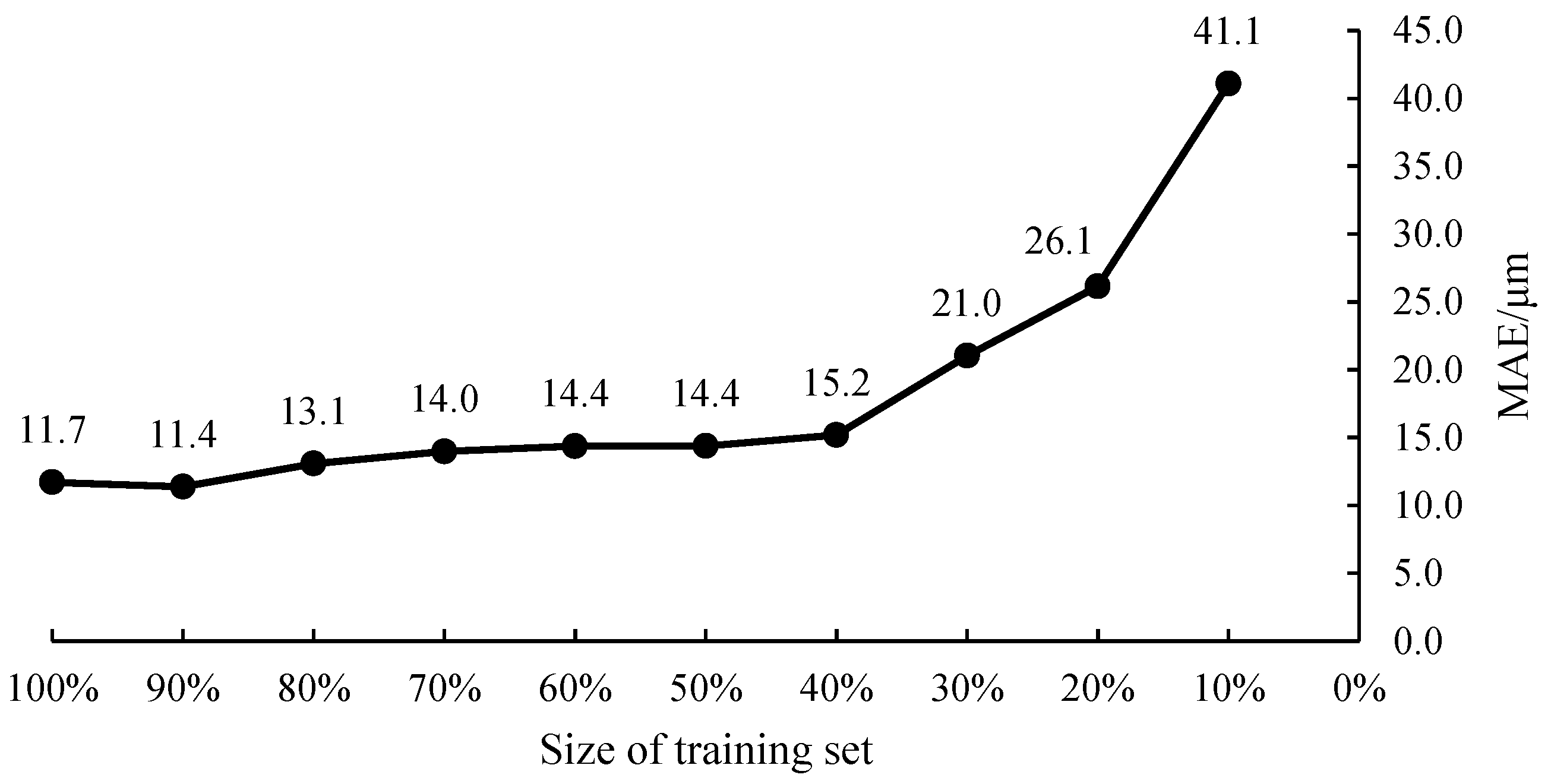
4.3. Impact of Dataset Size on Model Performance

Next, the impact of the size of the training dataset on the model’s diagnostic accuracy is analyzed. Based on the original dataset (containing 29,187 samples), the training set size is randomly reduced by 10% each time and model testing is conducted again. The size of the validation set is reduced synchronously with the test set, and k-fold cross-validation (k = 5) is still used to randomly divide the validation set. The size of the test set remains unchanged, always maintaining 1400 samples. The test results are shown in Table 4, and the trend of MAE on the test set with respect to the size of the training set is shown in Figure 16.
The MAE for 100% training set size is already given in Table 2. As the number of training set samples decreases, the error gradually increases, but the change trend is relatively slow between 100% and 40%, while between 40% and 10%, the diagnostic error increases significantly. From the results, it can be seen that for the established MGCNN model, a larger and more complete training set can better train the model. To ensure the generalization ability of the model, there is a roughly defined “lower limit” for the training set size. Taking Table 4 as an example, the model accuracy is similar above 40% data volume, while it significantly deteriorates below 40%. Considering the cost of data collection and processing, 40% data volume would be a suitable choice. Generally speaking, as the complexity of the model increases and the number of parameters to be trained increases, the demand for the scale of the dataset will also increase. Due to significant variations in data distribution across different environments, appropriately estimating the data volume based on specific conditions and requirements will aid in the deployment and application of the model.

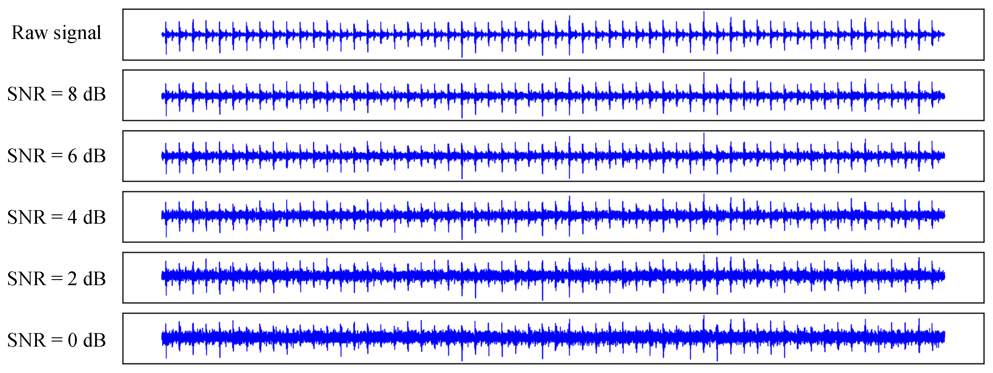
4.4. Impact of Noise on Model Performance

This section analyzes the impact of noise on MGCNN by adding noise to datasets at various signal-to-noise ratio (SNR) levels. The definition of SNR is as follows [52]:
SNR = 10 lg P s P n
where P s is the signal power, and P n is the noise power. A lower SNR indicates a higher noise component. Five noise levels were chosen, specifically SNR = [8 dB, 6 dB, 4 dB, 2 dB, 0 dB], and Figure 17 shows the waveform of a signal after the addition of different noise levels.
It is worth noting that three specific noise strategies were implemented. Each strategy includes test results for five SNRs:
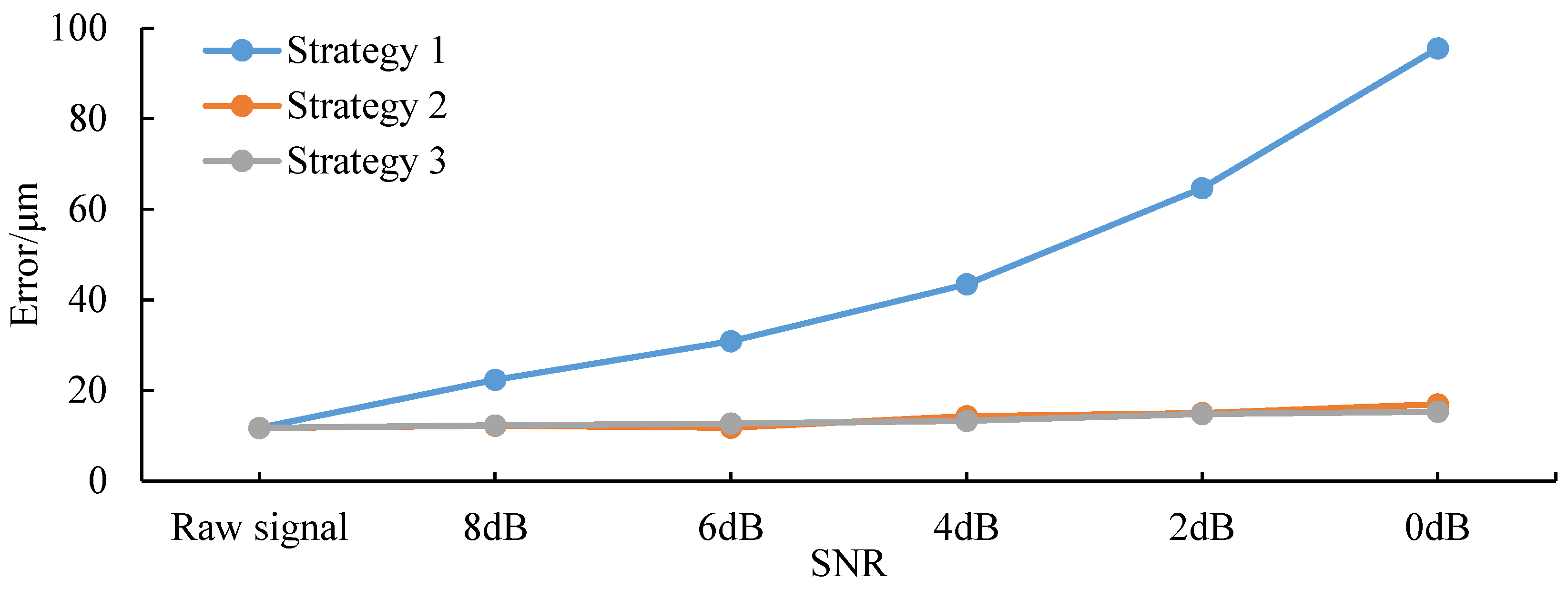
  • Strategy 1: Noise at a specific SNR was not added to the training or validation sets but only to the test set. The test results are shown in Table 5.
  • Strategy 2: Noise at a specific SNR was added to all training, validation, and test sets. The test results are shown in Table 6.
  • Strategy 3: Noise at one specific SNR was added to the test set, while the remaining four SNRs were added to the training and validation sets. For example, the test set was subjected to 0 dB of noise, whereas the training and validation sets were exposed to noise levels of SNR = [8 dB, 6 dB, 4 dB, 2 dB], resulting in a quadrupling of the training set size. The test results are shown in Table 7.
The comparison of errors for the three noise strategies is illustrated in Figure 18. As the SNR decreases, meaning the noise increases, the error in Strategy 1 shows a significant increasing trend, while in Strategy 2, since the noise level added to both the training and test sets is the same, meaning the data distribution is identical, the error only slightly increases with the addition of noise, remaining within an acceptable range. On the other hand, in Strategy 3, where the SNR in the training set differs from that in the test set, thus leading to different data distributions, the error trend is similar to that of Strategy 2. This indicates that data augmentation through the addition of varying levels of noise to the training set can effectively enhance the model’s robustness. In practical applications, it is often difficult to know the noise distribution of the test targets a priori; therefore, Strategy 3 presents an effective method for data augmentation and holds certain practical value.

4.5. Prognosis of Remaining Useful Life

Based on the diagnosis of MWD, this section theoretically predicts the remaining useful life (RUL) of sliding bearings. RUL is defined as the time interval from the current moment to the future failure moment [59]. We establish D threshold as the failure threshold for the sliding bearing; when MWD reaches D threshold , the bearing is considered to have failed. We recorded the actual MWD change curve for a wear test, as illustrated in Figure 19. Setting D threshold = 1000 μ m , we use the diagnostic results at various depths and corresponding times to fit an exponential function [60], as shown in Equation (19). The time at which this fitted curve reaches the failure threshold is taken as the predicted failure time.
D = a · exp ( b t ) a
where a and b are parameters to be determined, obtained through least squares fitting. Then, the predicted RUL can be calculated:
RUL = 1 b ln ( D threshold a 1 ) t i
where t i is the current time. When the MWD diagnostic result changes, the parameters a and b are updated, and the RUL prediction results are revised accordingly. The prediction results and errors of RUL are shown in Table 8.
In the early stages of prediction, due to the limited data available for fitting, the RUL predictions can exhibit significant errors. As the bearing continues to operate and diagnostic results are updated, the accuracy of the predictions improves, and the error tends to decrease towards zero. This indicates that the method is theoretically viable for predicting the RUL of sliding bearings. During the initial stages when prediction errors are large, it is advisable to make comprehensive judgments by integrating more conditions according to actual situations to avoid misjudgments. Meanwhile, it must be acknowledged that the validation experiments conducted in this study are relatively simplistic. Future research could involve using more accurate degradation models and developing failure conditions that are better suited to different practical scenarios.

5. Conclusions

This paper addresses the quantitative diagnosis of wear in sliding bearings and proposes an intelligent diagnostic method based on an MGCNN. The proposed method utilizes dual-path parallel structures in the time and frequency domains to process time-domain and frequency-domain signals separately, ensuring the integrity of information transmission through residual network connections. Within the constructed MGC module, three parallel channels, including long-term, medium-term, and short-term cycles, are employed to extract multiscale cyclic information from bearing vibration signals. Additionally, nonlinear gated units are used to adaptively adjust the weights during the feature information transmission process, enhancing the model’s representation and generalization capabilities. The experimental results demonstrate that the proposed MGCNN model surpasses traditional CNN models and shallow machine learning models like SVR in terms of diagnostic performance. The proposed method can achieve high-precision, real-time wear diagnostics based on vibration signals and has preliminarily realized the RUL prediction of sliding bearings, consistent with expectations. Additionally, our experiments analyzed the impact of noise and data volume on model performance and provided practical noise augmentation strategies.
This research provides new insights and perspectives into the problem of sliding bearing wear diagnosis, yet it also reveals several limitations and challenges that remain. In terms of data collection, the current validation was conducted under laboratory conditions, assuming that the vibration signals were primarily due to gaps caused by bearing wear; however, in real-world engineering applications, vibration signals from other components may overlap, necessitating the separation of bearing signals from overall machine signals. Moreover, this study was validated at a single rotational speed; future research could explore more complex operating conditions, including the transferability of models between different conditions. Additionally, the proposed method, as a diagnostic approach based on vibration signals, fundamentally involves extracting features from periodic time series signals and performing regression fitting. Therefore, it possesses a certain universality in rotating equipment, presenting a broader potential for application. However, it should be noted that we used MWD as a quantifiable indicator in our current experiments because it meets intuitive expectations and is easily verifiable; when applying this methodology to other rotating elements, defining an appropriate state quantification indicator will be crucial. In future work, we aim to continually refine this method to adapt to more complex environments and enhance its impact on equipment status diagnosis and predictive maintenance.

Author Contributions

Conceptualization, J.D. and L.T.; methodology, J.D.; software, J.D.; validation, J.D., L.T. and H.C.; formal analysis, J.D.; investigation, J.D. and H.C.; resources, L.T.; data curation, J.D. and H.C.; writing—original draft preparation, J.D.; writing—review and editing, J.D. and L.T.; visualization, J.D.; supervision, L.T.; project administration, L.T. and J.D.; funding acquisition, L.T. All authors have read and agreed to the published version of the manuscript.

Funding

This research was funded by the National Key Research and Development Program of China, grant number 2020YFB1709103; the Beijing Municipal Natural Science Foundation, grant number 3182012; the Tsinghua University Initiative Scientific Research Program, grant number 2018Z05JZY006.

Data Availability Statement

The raw data supporting the conclusions of this article will be made available by the authors on request.

Conflicts of Interest

The authors declare no conflicts of interest.

References

  1. Ozsarac, U.; Findik, F.; Durman, M. The wear behaviour investigation of sliding bearings with a designed testing machine. Mater. Des. 2007, 28, 345–350. [Google Scholar] [CrossRef]
  2. Du, F.; Li, D.; Sa, X.; Li, C.; Yu, Y.; Li, C.; Wang, J.; Wang, W. Overview of friction and wear performance of sliding bearings. Coatings 2022, 12, 1303. [Google Scholar] [CrossRef]
  3. Shi, G.; Yu, X.; Meng, H.; Zhao, F.; Wang, J.; Jiao, J.; Jiang, H. Effect of surface modification on friction characteristics of sliding bearings: A review. Tribol. Int. 2023, 177, 107937. [Google Scholar] [CrossRef]
  4. Wang, L.; Kong, X.; Yu, G.; Li, W.; Li, M.; Jiang, A. Error estimation and cross-coupled control based on a novel tool pose representation method of a five-axis hybrid machine tool. Int. J. Mach. Tools Manuf. 2022, 182, 103955. [Google Scholar] [CrossRef]
  5. Luo, R.; Cao, P.; Dai, Y.; Fu, Y.; Zhao, F.; Huang, Y.; Yang, Q. Rotating machinery fault diagnosis theory and implementation. Instrum. Tech. Sens. 2014, 3, 107–110. [Google Scholar]
  6. Li, Y.; Tan, Y.; Ma, L.; Yao, J.; Zhang, Z. Wear reliability modeling and simulation analysis of ceramic plain bearing. Lubr. Eng. 2023, 48, 167–171. [Google Scholar]
  7. Bigoni, C.; Hesthaven, J.S. Simulation-based Anomaly Detection and Damage Localization: An application to Structural Health Monitoring. Comput. Methods Appl. Mech. Eng. 2020, 363, 112896. [Google Scholar] [CrossRef]
  8. Saxena, A.; Goebel, K.; Simon, D.; Eklund, N. Damage propagation modeling for aircraft engine run-to-failure simulation. In Proceedings of the 2008 International Conference on Prognostics and Health Management, Denver, CO, USA, 6–9 October 2008; IEEE: Piscataway, NJ, USA, 2008; pp. 1–9. [Google Scholar]
  9. Nectoux, P.; Gouriveau, R.; Medjaher, K.; Ramasso, E.; Chebel-Morello, B.; Zerhouni, N.; Varnier, C. PRONOSTIA: An experimental platform for bearings accelerated degradation tests. In Proceedings of the IEEE International Conference on Prognostics and Health Management, PHM’12, Minneapolis, MN, USA, 23–27 September 2012; pp. 1–8. [Google Scholar]
  10. Lei, Y.; Han, T.; Wang, B.; Li, N.; Yan, T.; Yang, J. XJTU-SY rolling element bearing accelerated life test datasets: A tutorial. J. Mech. Eng. 2019, 55, 1–6. [Google Scholar]
  11. Vencl, A.; Gašić, V.; Stojanović, B. Fault Tree Analysis of Most Common Rolling Bearing Tribological Failures. In Proceedings of the IOP Conference Series: Materials Science and Engineering, Galati, Romania, 22–24 September 2016; IOP Publishing: Bristol, UK, 2017; Volume 174, p. 012048. Available online: https://iopscience.iop.org/article/10.1088/1757-899X/174/1/012048 (accessed on 10 April 2024).
  12. Li, H.; Zhang, Q.; Qin, X.; Sun, Y. Fault diagnosis method for rolling bearings based on short-time Fourier transform and concolution neural network. J. Vib. Shock 2018, 37, 124–131. [Google Scholar]
  13. Han, T.; Liu, C.; Yang, W.; Jiang, D. Deep transfer network with joint distribution adaptation: A new intelligent fault diagnosis framework for industry application. ISA Trans. 2020, 97, 269–281. [Google Scholar] [CrossRef]
  14. Wang, B.; Lei, Y.; Li, N.; Li, N. A hybrid prognostics approach for estimating remaining useful life of rolling element bearings. IEEE Trans. Reliab. 2020, 69, 401–412. [Google Scholar] [CrossRef]
  15. Zhu, B.; Wang, L.; Wu, J.; Lai, H. Reliability modeling and evaluation of CNC machine tools for a general state of repair. J. Tsinghua Univ. Sci. Technol. 2022, 62, 965–970. [Google Scholar]
  16. Wang, L.; Zhu, B.; Wu, J.; Tao, Z. Fault analysis of circular tool magazine based on Bayesian network. J. Jilin Univ. Eng. Technol. Ed. 2022, 52, 280–287. [Google Scholar]
  17. Luo, J. New Techniques of Influencing the Development of Manuvacturing Industry. Res. China Mark. Regul. 2020, 12–14. [Google Scholar]
  18. Alexander, P.; Evgeny, T. Procedure for simulation of stable thermal conductivity of bearing assemblies. Adv. Eng. Lett. 2023, 2, 58–63. [Google Scholar] [CrossRef]
  19. Baron, P.; Pivtorak, O.; Ivan, J.; Kočiško, M. Assessment of the Correlation between the Monitored Operating Parameters and Bearing Life in the Milling Head of a CNC Computer Numerical Control Machining Center. Machines 2024, 12, 188. [Google Scholar] [CrossRef]
  20. Wen, S. Study on lubrication theory-progress and thinking-over. Tribology 2007, 6, 497–503. [Google Scholar]
  21. Yang, J.; Yang, S.; Chen, C.; Wang, Y.; Wu, W. Rearch on sliding bearings and rotor system stability. J. Aerosp. Power 2008, 23, 1420–1426. [Google Scholar]
  22. Martsinkovsky, V.; Yurko, V.; Tarelnik, V.; Filonenko, Y. Designing thrust sliding bearings of high bearing capacity. Procedia Eng. 2012, 39, 148–156. [Google Scholar] [CrossRef]
  23. Chasalevris, A.C.; Nikolakopoulos, P.G.; Papadopoulos, C.A. Dynamic effect of bearing wear on rotor-bearing system response. J. Vib. Acoust. 2013, 135, 011008. [Google Scholar] [CrossRef]
  24. Lin, L.; He, M.; Ma, W.; Wang, Q.; Zhai, H.; Deng, C. Dynamic Characteristic Analysis of the Multi-Stage Centrifugal Pump Rotor System with Uncertain Sliding Bearing Structural Parameters. Machines 2022, 10, 473. [Google Scholar] [CrossRef]
  25. Tang, D.; Xiang, G.; Guo, J.; Cai, J.; Yang, T.; Wang, J.; Han, Y. On the optimal design of staved water-lubricated bearings driven by tribo-dynamic mechanism. Phys. Fluids 2023, 35, 093611. [Google Scholar] [CrossRef]
  26. Tofighi-Niaki, E.; Safizadeh, M.S. Dynamic of a flexible rotor-bearing system supported by worn tilting journal bearings experiencing rub-impact. Lubricants 2023, 11, 212. [Google Scholar] [CrossRef]
  27. Yang, T.; Xiang, G.; Cai, J.; Wang, L.; Lin, X.; Wang, J.; Zhou, G. Five-DOF nonlinear tribo-dynamic analysis for coupled bearings during start-up. Int. J. Mech. Sci. 2024, 296, 109068. [Google Scholar] [CrossRef]
  28. Sun, J.; Zhu, X.; Zhang, L.; Wang, X.; Wang, C.; Wang, H.; Zhao, X. Effect of surface roughness, viscosity-pressure relationship and elastic deformation on lubrication performance of misaligned journal bearings. Ind. Lubr. Tribol. 2014, 66, 337–345. [Google Scholar] [CrossRef]
  29. Engel, T.; Lechler, A.; Verl, A. Sliding bearing with adjustable friction properties. Cirp-Ann.-Manuf. Technol. 2016, 65, 353–356. [Google Scholar] [CrossRef]
  30. Ren, G. A new method to calculate water film stiffness and damping for water lubricated bearing with multiple axial grooves. Chin. J. Mech. Eng. 2020, 33, 1–18. [Google Scholar] [CrossRef]
  31. Tang, D.; Xiao, K.; Xiang, G.; Cai, J.; Fillon, M.; Wang, D.; Su, Z. On the nonlinear time-varying mixed lubrication for coupled spiral microgroove water-lubricated bearings with mass conservation cavitation. Tribol. Int. 2024, 193, 109381. [Google Scholar] [CrossRef]
  32. Ojala, N.; Valtonen, K.; Heino, V.; Kallio, M.; Aaltonen, J.; Siitonen, P.; Kuokkala, V.T. Effects of composition and microstructure on the abrasive wear performance of quenched wear resistant steels. Wear 2014, 317, 225–232. [Google Scholar] [CrossRef]
  33. Liu, Y.; Ma, G.; Zhu, L.; Wang, H.; Han, C.; Li, Z.; Wang, H.; Yong, Q.; Huang, Y. Structure–performance evolution mechanism of the wear failure process of coated spherical plain bearings. Eng. Fail. Anal. 2022, 135, 106097. [Google Scholar] [CrossRef]
  34. Kumar Rajak, S.; Kumar, D.; Seetharam, R.; Tandon, P. Mechanical and dry sliding wear analysis of porcelain reinforced SAE660 bronze bearing alloy composite fabricated by stir casting method. Mater. Today Proc. 2023, 87, 210–214. [Google Scholar] [CrossRef]
  35. Yin, Y.; Jiao, M.; Xie, T.; Zheng, Z.; Liu, K.; Yu, J.; Tian, M. Research progress in sliding bearing materials. Lubr. Eng. 2006, 183–187. [Google Scholar]
  36. Jeon, H.G.; Cho, D.H.; Yoo, J.H.; Lee, Y.Z. Wear Prediction of Earth-Moving Machinery Joint Bearing via Correlation between Wear Coefficient and Film Parameter: Experimental Study. Tribol. Trans. 2018, 61, 808–815. [Google Scholar] [CrossRef]
  37. König, F.; Ouald Chaib, A.; Jacobs, G.; Sous, C. A multiscale-approach for wear prediction in journal bearing systems—From wearing-in towards steady-state wear. Wear 2019, 426-427, 1203–1211. [Google Scholar] [CrossRef]
  38. Dai, J.; Tian, L. A Novel Prognostic Method for Wear of Sliding Bearing Based on SFENN. In Proceedings of the Intelligent Robotics and Applications, Hangzhou, China, 5–7 July 2023; Yang, H., Liu, H., Zou, J., Yin, Z., Liu, L., Yang, G., Ouyang, X., Wang, Z., Eds.; Springer Nature: Singapore, 2023; pp. 212–225. [Google Scholar]
  39. Cao, H.; Niu, L.; Xi, S.; Chen, X. Mechanical model development of rolling bearing-rotor systems: A review. Mech. Syst. Signal Process. 2018, 102, 37–58. [Google Scholar] [CrossRef]
  40. Zhang, H.; Cisse, M.; Dauphin, Y.N.; Lopez-Paz, D. mixup: Beyond empirical risk minimization. arXiv 2017, arXiv:1710.09412. [Google Scholar]
  41. Humeau-Heurtier, A. The multiscale entropy algorithm and its variants: A review. Entropy 2015, 17, 3110–3123. [Google Scholar] [CrossRef]
  42. Chen, S.; Shang, P. Financial time series analysis using the relation between MPE and MWPE. Phys. A Stat. Mech. Appl. 2020, 537, 122716. [Google Scholar] [CrossRef]
  43. Petrauskiene, V.; Ragulskiene, J.; Zhu, H.; Wang, J.; Cao, M. The discriminant statistic based on MPE-MWPE relationship and non-uniform embedding. J. Meas. Eng. 2022, 10, 150–163. [Google Scholar] [CrossRef]
  44. Krizhevsky, A.; Sutskever, I.; Hinton, G.E. Imagenet classification with deep convolutional neural networks. Adv. Neural Inf. Process. Syst. 2012, 25. [Google Scholar] [CrossRef]
  45. LeCun, Y.; Bengio, Y.; Hinton, G. Deep learning. Nature 2015, 521, 436–444. [Google Scholar] [CrossRef] [PubMed]
  46. Glorot, X.; Bengio, Y. Understanding the difficulty of training deep feedforward neural networks. In Proceedings of the Thirteenth International Conference on Artificial Intelligence and Statistics, JMLR Workshop and Conference Proceedings, Chia Laguna Resort, Sardinia, Italy, 13–15 May 2010; pp. 249–256. [Google Scholar]
  47. Glorot, X.; Bordes, A.; Bengio, Y. Deep sparse rectifier neural networks. In Proceedings of the Fourteenth International Conference on Artificial Intelligence and Statistics, JMLR Workshop and Conference Proceedings, Fort Lauderdale, FL, USA, 11–13 April 2011; pp. 315–323. [Google Scholar]
  48. Cybenko, G. Approximation by superpositions of a sigmoidal function. Math. Control. Signals Syst. 1989, 2, 303–314. [Google Scholar] [CrossRef]
  49. Hornik, K. Approximation capabilities of multilayer feedforward networks. Neural Netw. 1991, 4, 251–257. [Google Scholar] [CrossRef]
  50. Bottou, L. Stochastic gradient descent tricks. In Neural Networks: Tricks of the Trade: Second Edition; Springer: Berlin/Heidelberg, Germany, 2012; pp. 421–436. [Google Scholar]
  51. Kingma, D.P.; Ba, J. Adam: A method for stochastic optimization. arXiv 2014, arXiv:1412.6980. [Google Scholar]
  52. Zhang, X. Modern Signal Processing; Walter de Gruyter GmbH & Co KG: Berlin, Germany, 2022. [Google Scholar]
  53. He, K.; Zhang, X.; Ren, S.; Sun, J. Identity mappings in deep residual networks. In Proceedings of the Computer Vision–ECCV 2016: 14th European Conference, Amsterdam, The Netherlands, 11–14 October 2016; Proceedings, Part IV 14. Springer: Berlin/Heidelberg, Germany, 2016; pp. 630–645. [Google Scholar]
  54. He, K.; Zhang, X.; Ren, S.; Sun, J. Deep residual learning for image recognition. In Proceedings of the IEEE Conference on Computer Vision and Pattern Recognition, Las Vegas, NV, USA, 27–30 June 2016; pp. 770–778. [Google Scholar]
  55. Srivastava, N.; Hinton, G.; Krizhevsky, A.; Sutskever, I.; Salakhutdinov, R. Dropout: A simple way to prevent neural networks from overfitting. J. Mach. Learn. Res. 2014, 15, 1929–1958. [Google Scholar]
  56. Szegedy, C.; Liu, W.; Jia, Y.; Sermanet, P.; Reed, S.; Anguelov, D.; Erhan, D.; Vanhoucke, V.; Rabinovich, A. Going deeper with convolutions. In Proceedings of the IEEE Conference on Computer Vision and Pattern Recognition, Boston, MA, USA, 7–12 June 2015; pp. 1–9. [Google Scholar]
  57. Dai, J.; Tian, L.; Han, T.; Chang, H. Digital Twin for wear degradation of sliding bearing based on PFENN. Adv. Eng. Inform. 2024, 61, 102512. [Google Scholar] [CrossRef]
  58. Lei, Y.; He, Z.; Zi, Y.; Hu, Q. Fault diagnosis of rotating machinery based on multiple ANFIS combination with GAs. Mech. Syst. Signal Process. 2007, 21, 2280–2294. [Google Scholar] [CrossRef]
  59. Jardine, A.K.; Lin, D.; Banjevic, D. A review on machinery diagnostics and prognostics implementing condition-based maintenance. Mech. Syst. Signal Process. 2006, 20, 1483–1510. [Google Scholar] [CrossRef]
  60. He, W.; Williard, N.; Osterman, M.; Pecht, M. Prognostics of lithium-ion batteries based on Dempster–Shafer theory and the Bayesian Monte Carlo method. J. Power Sources 2011, 196, 10314–10321. [Google Scholar] [CrossRef]
Figure 1. (a) Rotor–bearing contact, where ω is the rotational speed, O b is the center of the bearing, O is the geometric center of rotor, μ is the surface friction coefficient, r 0 is the original radius of bearing inner surface, and F n is the normal pressure; (b) dynamic system of the rotor–bearing, where m is the mass of rotor and O is the geometric center of the rotor, while O is the center of mass, e = O O represents the eccentricity, and k and c are the equivalent stiffness and damping, respectively.
Machines 12 00266 g001
Figure 2. The process of sample cutting.
Machines 12 00266 g002
Figure 3. The process of convolution. The symbol (*) represents convolution operation, and the different colors represent parameters at different depths of the convolution kernel.
Machines 12 00266 g003
Figure 4. The process of max pooling. The different colors represent different pooling regions.
Machines 12 00266 g004
Figure 5. (a) Tanh. (b) Sigmoid. (c) ReLU.
Machines 12 00266 g005
Figure 6. Structure of the neuron.
Machines 12 00266 g006
Figure 7. Structure of the MGCNN. The different colors in MGC represent different cycle channels.
Machines 12 00266 g007
Figure 8. The process of the gated unit.
Machines 12 00266 g008
Figure 9. (a) Bearing housing assembly in wear test; (b) bearing housing assembly in vibration test; (c) overall structure of the test platform [57].
Machines 12 00266 g009
Figure 10. Sliding bearing test platform [57].
Machines 12 00266 g010
Figure 11. The worn bearing.
Machines 12 00266 g011
Figure 12. The measured vibration signals at different maximum wear depths.
Machines 12 00266 g012
Figure 13. The curve of validation set loss function during training.
Machines 12 00266 g013
Figure 14. The CNN model used for comparison.
Machines 12 00266 g014
Figure 15. Comparison of diagnosis results from different models, where the abscissa corresponds to [0, 70, 240, 270, 410, 420, 530, 690, 740, 760, 900, 950, 1060, 1160] sequentially.
Machines 12 00266 g015
Figure 16. The variation in diagnosis error with training set size.
Machines 12 00266 g016
Figure 17. Signal with Gaussian white noise added at different SNRs, where D = 420 μ m and the signal length is 1 s.
Machines 12 00266 g017
Figure 18. Comparison of errors for the three noise strategies.
Machines 12 00266 g018
Figure 19. The actual degradation curve and the fitting curves at different times.
Machines 12 00266 g019
Table 1. Parameters of MGCNN.
LayerNumber of ChannelsConvolution KernelMax PoolingGated Unit
InputOutputSizeStrideSizeStride
1 st -MGC
(time-domain)
Long-term cycle116129 × 11
1 st -ConvMedium-term cycle11633 × 114 × 12Sigmoid
Short-term cycle1169 × 11
2 nd -Conv16165 × 124 × 12/
Res-connection1481 × 18///
2 nd -MGC
(time-domain)
Long-term cycle4816129 × 11
1 st -ConvMedium-term cycle481633 × 114 × 12Sigmoid
Short-term cycle48169 × 11
2 nd -MGC in time-domain16165 × 124 × 12/
Res-connection48481 × 18///
1 st -MGC
(frequency-domain)
Long-term cycle116129 × 11
1 st -ConvMedium-term cycle11633 × 114 × 12Sigmoid
Short-term cycle1169 × 11
2 nd -Conv16165 × 124 × 12/
Res-connection1481 × 18///
2 nd -MGC
(frequency-domain)
Long-term cycle4816129 × 11
1 st -ConvMedium-term cycle481633 × 114 × 12Sigmoid
Short-term cycle48169 × 11
2 nd -Conv16165 × 124 × 12/
Res-connection48481 × 18///
MLPFlattenChannels: 48→1; activation function: ReLU; Dropout = 0.5
1st layerLength of feature vectors: 2304→20; activation function: ReLU
2nd layerLength of feature vectors: 20→1; activation function: ReLU
Table 2. Comparison of wear depth diagnosis results. Here, SVR-1 represents the SVR model using time–frequency domain features, while SVR-2 represents the SVR model using time-domain features.
True Value/ μ mMGCNNCNNSVR-1SVR-2
OutputErrorOutputErrorOutputErrorOutputError
00.70.715.815.8322.5322.5148.7148.7
7085.815.8100.130.1371.3301.3178108
240230.4−9.6219.5−20.5385.0145.0226.6−13.4
270302.832.8338.668.6408.6138.6321.351.3
410427.617.6397.2−12.8417.87.8332.8−77.2
420404.9−15.1410.5−9.5428.68.6452.632.6
530514.2−15.8544.514.5435.1−94.9431.7−98.3
690682.8−7.2654.4−35.6441.8−248.2586.7−103.3
740738.0−2.0736.3−3.7448.6−291.4734.8−5.2
760759.1−0.9779.419.4449.2−310.8778.618.6
900899.7−0.3911.111.1473.8−426.2873.4−26.6
950968.618.6973.623.6478.5−471.51011.661.6
10601072.412.41072.612.6489.1−570.91094.834.8
11601144.9−15.11116.7−43.3478.0−6821060.8−99.2
MAE11.722.9287.162.8
Table 3. The diagnosis results of MGCNN. The test set consists of data from three bearings with wear depths of [240 μ m , 530 μ m , 760 μ m ], respectively.
True Value/ μ mMGCNNCNNSVR-1SVR-2
OutputErrorOutputErrorOutputErrorOutputError
240176.9−63.1184.4−55.6390.1150.1131.5−108.5
530557.427.4584.054.0428.2−101.8363.2−166.8
760797.437.4808.048.0448.1−311.9846.386.3
MAE42.652.4187.9120.5
Table 4. Diagnostic results of MGCNN with different sizes of training set.
True ValueSize of Training Set
90%80%70%60%50%40%30%20%10%
01.15.14.72.46.68.29.933.266.1
7091.884.686.793.486.397.3111.3108.5131.9
240237.1234.5231.7235.3231.7233.0218.5202.8199.4
270302.4307.7302.8306.3311.4311.2327.1327.7331.6
410421.3422.1428.4430.2428.8410.5405.1406.7369.3
420402.0404.4403.1403.5402.1408.1420.4420.1453.6
530520.6516.2517.4518.5519.6517.1520.3527.8529.3
690678.8685.8682.5683.1683.0684.4673.9664.5651.1
740735.4733.2733.9731.6732.8734.2734.6731.5741.4
760760.7763.6761.3763.5763.1769.2778.5788.1817.1
900903.5905.2904.5905.4907.8908.9919.8918.4939.1
950973.1975.9979.1976.1970.3977.1981.9996.9999.6
10601067.11074.11075.71075.31075.71074.41081.81087.21105.7
11601147.71140.91138.81139.61139.51127.21123.91120.61121.9
MAE11.413.114.014.414.415.221.026.141.1
Table 5. Test results under Strategy 1.
Models in k-Fold Cross-ValidationRaw SignalSNR
8 dB6 dB4 dB2 dB0 dB
No.1/23.030.240.156.780.0
No.2/21.230.243.766.1101.1
No.3/22.332.046.367.799.6
No.4/23.330.842.766.5102.9
No.5/22.031.244.466.494.2
Mean11.722.430.943.464.795.6
Table 6. Test results under Strategy 2.
Models in k-Fold Cross-ValidationRaw SignalSNR
8 dB6 dB4 dB2 dB0 dB
No.1/11.610.014.014.616.4
No.2/13.413.215.015.817.5
No.3/12.712.113.814.217.5
No.4/12.411.615.415.515.7
No.5/10.811.812.914.817.4
Mean11.712.211.714.215.016.9
Table 7. Test results under Strategy 3.
Models in k-Fold Cross-ValidationRaw SignalSNR
8 dB6 dB4 dB2 dB0 dB
No.1/11.912.714.313.915.4
No.2/11.314.513.813.914.6
No.3/13.012.713.814.515.6
No.4/12.212.510.515.517.1
No.5/12.910.813.716.113.6
Mean11.712.212.613.214.815.3
Table 8. Prognosis of RUL.
Current Time t i (min)Actual RUL (min)Predicted RUL (min)Error (min)
01707−163
3413614−122
779312027
809069−21
1046652−14
124465812
146245733
150203515
151192910
16192617
16731310
170044
Disclaimer/Publisher’s Note: The statements, opinions and data contained in all publications are solely those of the individual author(s) and contributor(s) and not of MDPI and/or the editor(s). MDPI and/or the editor(s) disclaim responsibility for any injury to people or property resulting from any ideas, methods, instructions or products referred to in the content.

